Edge exchangeable models for network dataThanks: H. Crane is partially supported by NSF grants CNS-1523785 and CAREER DMS-1554092.

Abstract.

Exchangeable models for vertex labeled graphs cannot replicate the large sample behaviors of sparsity and power law degree distributions observed in many network datasets. Out of this mathematical impossibility emerges the question of how network data can be modeled in a way that reflects known empirical behaviors and respects basic statistical principles. We address this question by observing that edges, not vertices, act as the statistical units in many network datasets, making a theory of edge labeled networks more natural for these applications. Within this context we introduce the new invariance principle of edge exchangeability, which unlike its vertex exchangeable counterpart admits models for networks with sparse and/or power law structure. With this, we settle a longstanding question in statistical network modeling. We characterize all edge exchangeable network models and establish their basic statistical properties. We identify a tractable two parameter family of distributions with suitable theoretical properties, which we demonstrate in estimation and prediction problems on real datasets.

1. Introduction

Statistical network analysis is hamstrung by the lack of an inferential framework that both admits sound models for network formation with observed empirical properties and facilitates statistical inference in the way of estimation, prediction, and testing. Network datasets emerging from a wide range of real world processes, such as communications [18, 26], collaborations [4, 25], and relationships [23, 33], exhibit common structural features, namely sparsity and power law degree distribution [1, 4, 15, 17, 20]. Such networks are typically represented by a graphical structure, with labels assigned arbitrarily for the purposes of distinguishing between units.

Two fundamental statistical principles guide the modeling of such data:

• “There should be consistency with known limiting behaviour.” [10, p. 5]

• “The sense of the model and the meaning of the parameter […] may not be affected by accidental or capricious choices such as sample size or experimental design.” [24, p. 1237]

Within our specific context, Principle (I) speaks to the need for models that replicate the asymptotic properties of sparsity and power law, while Principle (II) recalls the logical necessity that inference is unhindered by arbitrary choices in the assignment of labels and subsampling mechanism used for data acquisition.

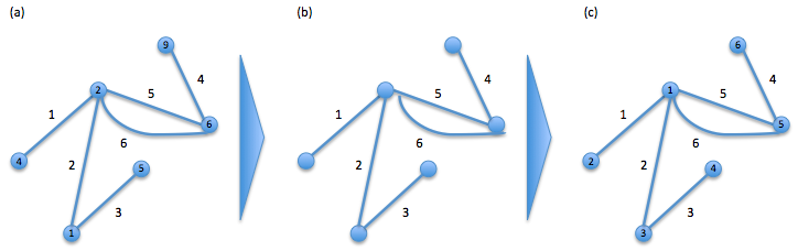
As is well known throughout the statistics and probability community, cf. [3, 5, 22], Principles (I) and (II) are not compatible under the conventional representation of network data by a graph with labeled vertices, as in Figure 1(b), and the corresponding notion of exchangeability with respect to vertex relabeling. Assuming a random graph for an infinite population of labeled vertices:

An exchangeable random graph is sparse if and only if it is empty, that is, has no edges, with probability 1.

Plainly, an exchangeable generating model, in the traditional sense, cannot exhibit essential logical properties in a way that respects well documented empirical behaviors.

Realizing the issue, Bickel and Chen [5] propose a class of exchangeable finite sample models that describe sparse sequences of finite graphs but are otherwise not consistent under subsampling. In so doing, they sacrifice Principle (II) by using a model for which the meaning of the parameter changes with the sample size. We discuss the implications of this approach further in Section 7.2.

As a heuristic explanation for why ordinary vertex exchangeability is untenable in most applications, we observe that many network datasets come about by a process of sampling interactions, that is, edges among individuals in a population. The vertices involved in those interactions are incidental to the interaction sampling scheme. From this point of view, the sampled vertices are not representative of the larger population—observed vertices are incident to sampled edges and, thus, tend to have higher than average degree—explaining why vertices cannot be labeled exchangeably in most applications.

With this observation, we settle a longstanding question of statistical network analysis by recognizing that the vast majority of network datasets arise by a process of interactions within a population, with the Enron email corpus [18] and actors collaboration network [30] as primary examples. In these cases, the edges correspond to the statistical units, justifying our development of the framework of edge exchangeable networks in Sections 4 and 5. In addition to resolving the larger statistical issues at play in network analysis, edge exchangeable models address a closely related question posed recently in the machine learning literature by Orbanz and Roy [27, p. 459]:

Is there a notion of probabilistic symmetry whose ergodic measures […] describe useful statistical models for sparse graphs with network properties?

We build our framework from first principles, with a formal definition of network data and basic network properties in Sections 2 and 3. In Section 4 we introduce edge exchangeability as the appropriate invariance for network data arising in a wide range of applications. In Section 5 we identify a two parameter family of edge exchangeable models with many theoretical properties suitable to statistical inference. Specifically, this model furnishes an explicit generating mechanism for edge exchangeable networks that exhibits sparse and power law behavior. In Section 6, we discuss issues of statistical inference from edge exchangeable models, including estimation, prediction, and testing, which we then demonstrate with several examples along the way. We discuss how the edge exchangeable framework differs from previous approaches at this problem in Section 7. We defer all proofs to Section 8, in which we also discuss and prove a characterization of the class of edge exchangeable network models with a de Finetti-type representation theorem.

2. Network data

Figure 1 depicts a network whose edges correspond to pairwise interactions between individuals in a population $\mathcal{P}$. A physical process of interactions generates the object in Figure 1(a). The process generally does not generate any vertex or edge labels, but labels are typically assigned after data generation in order to distinguish among statistical units and facilitate data analysis. The labeled versions in Figures 1(b) and 1(c) show two possible ways to represent the network data from Figure 1(a) by labeling its vertices and edges, respectively.

In the actors collaboration networks [4, 30], $\mathcal{P}$ consists of all movie actors and each movie corresponds to an interaction involving the set of individuals in its cast. In the Enron network [18] edges correspond to emails exchanged between Enron employees. Both of these examples produce networks with multiple edges and edges indexed by more than two vertices: in general there are more than two actors in each movie and nothing precludes a set of actors from being cast together in more than one movie; likewise, emails can involve more than two individuals and an email exchange between the same group of individuals can occur repeatedly over time. Analogous observations are true of many other network datasets; see Table 1.

To cover the range of datasets with these properties, we define network data as an association between a set of interactions, for example, movies or emails, and subsets of a population, for example, actors or employees, respectively. In general, an interaction can involve any finite subset of individuals from $\mathcal{P}$, and so we write $\mathop{\text{fin}}\nolimits(\mathcal{P})$ to denote the set of all finite subsets of $\mathcal{P}$.

Definition 2.1 (Network data).

Let $\mathcal{I}$ be a set of interactions among elements in a population $\mathcal{P}$. Network data is a function $E:\mathcal{I}\to\mathop{\text{fin}}\nolimits(\mathcal{P})$ associating each $i\in\mathcal{I}$ to the subset $E(i)\subset\mathcal{P}$ of elements involved in interaction $i$.

Remark 2.2.

If we instead interpret $\mathcal{I}$ as a set of events, then we could extend Definition 2.1 by defining network data as a function $E:\mathcal{I}\to\mathop{\text{fin}}\nolimits(\mathop{\text{fin}}\nolimits(\mathcal{P}))$, where now $E(i)=\{A,A^{\prime}\}$, for $A,A^{\prime}\subset\mathcal{P}$, means that event $i$ occurred separately to the set of individuals in $A$ and $A^{\prime}$. Below we stick to Definition 2.1 because this more general setting serves no purpose in any of the applications we consider.

Definition 2.1 encompasses the most common representation of network data for which each interaction involves exactly two vertices. For simplicity, all our figures specialize to this case of binary interactions. The general definition above serves a practical purpose in our analysis of the actors collaboration network, which cannot be represented by a network with binary edges.

Our definition also captures subtle features of network data that the more conventional representation by a graph $G=(\mathcal{P},\mathcal{E})$, with vertex set $\mathcal{P}$ and edge set $\mathcal{E}\subseteq\mathop{\text{fin}}\nolimits(\mathcal{P})$, does not. In statistical practice, labeling the vertices, as in Figure 1(b), underlies the assumption that the vertices are the statistical units for the intended application. Aside from Kolaczyk [19, p. 54], who states it explicitly, this assumption about units is implicit in all other studies of network models. In many situations, including all examples in Table 1, the interactions, and thus the edges, act as the statistical units, as Definition 2.1 makes clear.

The representation of network data by a vertex labeled graph also suggests that network data comes about by observing all interactions among individuals in a sample $\mathcal{S}\subset\mathcal{P}$, an assumption which is plainly false in many applications. In the actors collaboration dataset, for example, the network data are obtained by sampling a set of movies and observing the set of actors in each movie. The sampled actors are those in the cast of at least one of the sampled movies. An actor, therefore, cannot be thought of in isolation from the set of movies in which he/she has acted.

The subtle distinction between the (real world) network in Figure 1(a) and the network data in Figures 1(b) and 1(c) elucidates the role of exchangeability as a logical principle rather than a computational or practical assumption made for the purpose of tractability. Network models should be invariant to relabeling units precisely because the labels are assigned exogenously to the real world process, and for no other reason. Definition 2.1 and our identification of edges as the units rightly shifts the focus from vertices to edges, foreshadowing why our notion of edge exchangeability in Definition 4.1 is a natural invariance principle for network modeling in this context.

Figure 1. (a) A network structure derived from some physical process. Neither vertices nor edges come equipped with labels. Labels are assigned exogenously during data analysis. (b) Network data obtained from the network in Panel (a) by labeling vertices. (c) Network data obtained from the network in Panel (a) by labeling edges.

3. Network properties

Principle (I) factors into network modeling by noting that sparsity and power law are asymptotic properties of a sequence of networks $(G_{n})_{n\geq 1}$ of growing size. For any network $G$, we define a sample size parameter $\mathop{\text{size}}\nolimits(G)$, which may be any reasonable measure of size, with the number of vertices and number of edges the most appropriate in most situations. In statistical applications, the sample size corresponds to the number of units under consideration, which is ordinarily taken to be the vertices in all previous statistical treatments of network data [19, p. 54], but as we alluded in Section 2 and expound further in Section 4, the edges act as the units in many applications.

Irrespective of labeling convention, we define $v(G)$ as the number of vertices, $e(G)$ as the number of edges, and $d(G)=(d_{k}(G))_{k\geq 0}$ as the degree distribution of a network $G$, where $d_{k}(G)$ is the proportion of vertices with degree $k$ in $G$ with $d_{k}(G)=N_{k}(G)/v(G)$ for $N_{k}(G)$ equal to the number of vertices incident to exactly $k$ edges. For example, the network data $G$ in Figure 1(a) has $v(G)=7$, $e(G)=6$, and $d(G)=(1/7,3/7,1/7,1/7,1/7)$.

Definition 3.1 (Sparsity and power law degree distribution).

Let $(G_{n})_{n\geq 1}$ be a sequence of networks with $\mathop{\text{size}}\nolimits(G_{n})=n$ for each $n\geq 1$. The sequence $(G_{n})_{n\geq 1}$ is sparse if

$$\limsup_{n\to\infty}\frac{e(G_{n})}{v(G_{n})^{2}}=0.$$

The sequence $(G_{n})_{n\geq 1}$ exhibits power law degree distribution if for some $\gamma>1$ the degree distributions $(d(G_{n}))_{n\geq 1}$ satisfy $d_{k}(G_{n})\sim L(k)k^{-\gamma}$ as $n\to\infty$ for all large $k$ for some slowly varying function $L(x)$, that is, $\lim_{x\to\infty}L(tx)/L(x)=1$ for all $t>0$, where $a_{n}\sim b_{n}$ indicates that $a_{n}/b_{n}\to 1$ as $n\to\infty$.

Sparsity and power law are properties of a sequence of networks $(G_{n})_{n\geq 1}$ of growing size. In applications, they are assumed to be inherent features of a physical process, which corresponds to a network $G:\mathcal{I}\to\mathop{\text{fin}}\nolimits(\mathcal{P})$. These properties manifest themselves in data by sampling $\mathcal{S}\subset\mathcal{I}$ and observing the domain restriction $G|_{\mathcal{S}}:\mathcal{S}\to\mathop{\text{fin}}\nolimits(\mathcal{P})$ with $G|_{\mathcal{S}}(s)=G(s)$ for each $s\in\mathcal{S}\subset\mathcal{I}$.

We identify the set of interactions $\mathcal{I}$ as a collection of infinitely many units, which we distinguish by labeling each distinctly in $\mathop{\mathbb{N}}\nolimits=\{1,2,\ldots\}$. Since labels are arbitrary, we identify any sample of $n$ units from $\mathop{\mathbb{N}}\nolimits$ by $[n]=\{1,\ldots,n\}$. The definitions of sparsity and power law extend to properties of a population network $G:\mathop{\mathbb{N}}\nolimits\to\mathop{\text{fin}}\nolimits(\mathcal{P})$. We call a network $G:\mathop{\mathbb{N}}\nolimits\to\mathop{\text{fin}}\nolimits(\mathcal{P})$ sparse, or say that it has power law degree distribution, if the sequence of sampled networks $(G|_{[n]})_{n\geq 1}$ satisfies the appropriate conditions of Definition 3.1. Any discussion of sparsity or power law behavior in a network dataset, therefore, makes implicit reference not only to a population network but also to a mechanism by which a sequence of networks of growing size comes about.

4. Edge exchangeable network models

Network datasets

	Growth type		Sampling type
network	edge	vertex	edge	vertex	none
Facebook	✓	✓	✓a
Political blogs	✓4	✓1	✓a
US Airport	✓2,4,5				✓
UC Irvine	✓4		✓
Actors	✓3,4		✓
Co-authorship	✓3		✓
Enron	✓3,4		✓
Karate Club	✓2,4,5				✓
Wikipedia	✓4		✓
US Power6					✓

Table 1. Catalog of common network datasets categorized according to their growth by addition of edges or vertices. See Section 8.3 for a detailed description of each dataset. A $\checkmark$ signifies that the network exhibits growth of a certain generic type, that is, vertex or edge growth. Superscripts indicate specific features of the network data or its generating mechanism for consideration in statistical modeling: (1) growth by preferential attachment, (2) projection of a network with multiple edges, (3) network with hyperedges, (4) network with multiple edges, (5) finite population size, and (6) network exhibits no growth. Sampling type: (a) ego-centric network obtained by first taking a small set of vertices and sampling the network by looking at the surrounding neighborhood of vertices.

Figure 2. Statistical operations on network data with labeled edges. Panel (a) is network data for a sample of five units labeled $1,\ldots,5$. Panel (b) shows the network from (a) relabeled according to permutation (1354)(26). Panel (c) shows the restriction of the network in (a) to the units labeled in $1,\ldots,4$.

With the exception of the Power Grid network, which is a fixed, physical network, all of the networks in Table 1 are driven by interactions within a population. The US Airport and Karate Club networks, though they do not exhibit vertex growth, still grow as a result of interactions between airports and club members, respectively. As the primary entities driving network structure, the edges naturally serve as the units in all of these cases.

With respect to Definition 2.1, we label the edges by $\mathop{\mathbb{N}}\nolimits$ and assume $E:\mathop{\mathbb{N}}\nolimits\to\mathop{\text{fin}}\nolimits(\mathcal{P})$ corresponds to a sequence $(E_{n})_{n\geq 1}$, where each $E_{n}:[n]\to\mathop{\text{fin}}\nolimits(\mathcal{P})$ is obtained by subsampling units $[n]\subset\mathop{\mathbb{N}}\nolimits$ and corresponds to the restriction $E|_{[n]}:[n]\to\mathop{\text{fin}}\nolimits(\mathcal{P})$ with $i\mapsto E(i)$ for each $i=1,\ldots,n$. In this setting, network data can be represented by an edge labeled network, as in Figure 1(c). Vertex labels convey no additional information since the vertices have no meaning outside the context their interactions with other vertices.

Given any permutation $\sigma:[n]\to[n]$, we write $E_{n}^{\sigma}=E_{n}\circ\sigma$ to denote the network data obtained from $E_{n}$ by reassigning unit labels according to $\sigma$, that is, $E_{n}^{\sigma}(i)=E_{n}(\sigma(i))$ for each $i=1,\ldots,n$. See Figure 2 for a visual illustration of the restriction and relabeling operations. As the network data arise from a process for unlabeled data as in Figure 1(a), the labels assigned to edges are arbitrary, suggesting the new notion of edge exchangeability.

Definition 4.1 (Edge exchangeability).

A random edge labeled network $Y:\mathop{\mathbb{N}}\nolimits\to\mathop{\text{fin}}\nolimits(\mathcal{P})$ is edge exchangeable, or simply exchangeable, if $Y^{\sigma}=_{\mathcal{D}}Y$ for all permutations $\sigma:\mathop{\mathbb{N}}\nolimits\to\mathop{\mathbb{N}}\nolimits$, where $=_{\mathcal{D}}$ denotes equality in distribution.

Edge exchangeable models assign the same probability to all edge labeled graphs that are equivalent up to relabeling, such as the two networks shown in Figure 3. Any random edge labeled network $Y:\mathop{\mathbb{N}}\nolimits\to\mathop{\text{fin}}\nolimits(\mathcal{P})$ gives rise to a compatible sequence of finite networks $(Y_{n})_{n\geq 1}$ by taking $Y_{n}=Y|_{[n]}$, the restriction by subsampling $[n]\subset\mathop{\mathbb{N}}\nolimits$ defined above. Any such sequence is infinitely edge exchangeable, meaning $Y_{n}^{\sigma}=_{\mathcal{D}}Y_{n}$ for all permutations $\sigma:[n]\to[n]$ and $Y_{n}|_{[m]}=_{\mathcal{D}}Y_{m}$ for all $n\geq m\geq 1$.

Our characterization of all edge exchangeable network models in Theorem 8.2 explains why vertices cannot be labeled exchangeably in networks that grow by a process of interactions in a population. While the arrival of edges occurs according to an exchangeable process, the vertices arrive in size biased order weighted by the relative frequency of their occurrence in interactions. The sample of vertices, therefore, does not represent an exchangeable draw from the population.

The representation in Theorem 8.2 likely has many further implications in the development of edge exchangeable network models, just as the analogous representation theorems of de Finetti and Aldous–Hoover do for exchangeable sequences and vertex labeled graphs, respectively. Most importantly, and in stark contrast to the more conventional setting of exchangeable networks with labeled vertices, edge exchangeable models admit sparse and power law behavior, as the two parameter model in Section 5 demonstrates.

Figure 3. Two edge labelings of the network data from Figure 1. An edge exchangeable model assigns equal probability to both networks. Vertices are not labeled and, therefore, vertex labels play no role in the exchangeability condition.

5. Two parameter edge exchangeable model

The two parameter edge exchangeable model below directly addresses our primary question of interest from Section 1. In addition to satisfying Principles (I) and (II), the model has a generative description which makes estimation and prediction tractable and affords a clear interpretation to model parameters.

5.1. Generating mechanism

Let $(\alpha,\theta)$ satisfy either $0<\alpha<1$ and $\theta>-\alpha$ or $\alpha<0$ and $\theta=-k\alpha$ for some $k=1,2,\ldots$. We generate a sequence $(Y_{n})_{n\geq 1}$ of edge labeled networks, where each $Y_{n}$ has $\mathop{\text{size}}\nolimits(Y_{n})=e(Y_{n})=n\geq 1$ as follows.

We initialize by choosing $Y_{1}$ among the two possible edge labeled graphs with one edge so that either $Y_{1}$ has a self-loop at a single vertex (with probability $(1-\alpha)/(\theta+1)$) or $Y_{1}$ has an edge between two distinct vertices (with probability $(\theta+\alpha)/(\theta+1)$). After $n$ steps, $Y_{n}$ has $n$ edges and a random number of vertices $N_{n}$. For the purpose of this construction only, we label these vertices arbitrarily $i=1,\ldots,N_{n}$ and write $D(i,n)$ to denote the total degree of vertex $i$ before the $(n+1)$st edge is added. (Note that each self-loop from a vertex to itself contributes 2 to its degree.) When the $(n+1)$st edge arrives, its two incident vertices $v_{1}(n+1)$ and $v_{2}(n+1)$ are chosen randomly among vertices labeled $1,\ldots,N_{n}$ and a new vertex $N_{n}+1$ as follows. With $N_{n}^{*}=N_{n}$, we first choose $v_{1}(n+1)$ randomly with probability

(1) $$\mathop{\text{pr}}\nolimits(v_{1}(n+1)=i)\propto\left\{\begin{array}[]{cc}D(i,n)-\alpha,&i=1,\ldots,N_{n}^{*}\\ \theta+\alpha N_{n}^{1},&i=N_{n}^{*}+1.\end{array}\right.$$

After choosing $v_{1}(n+1)$, we update $N_{n}^{*}$ according to whether or not $v_{1}(n+1)$ is a newly observed vertex: if $v_{1}(n+1)=N_{n}^{*}+1$, then we define $N_{n}^{\prime}=N_{n}^{*}+1$; otherwise, we put $N_{n}^{\prime}=N_{n}^{*}$. We then choose $v_{2}(n+1)$ as in (1) with $N_{n}^{*}=N_{n}^{\prime}$. When generating a network with directed edges, we orient edges to point from $v_{1}(n)$ to $v_{2}(n)$; in the undirected case, the edge between $v_{1}(n)$ and $v_{2}(n)$ has no orientation. We write $Y_{n}$ to denote the edge labeled network by removing vertex labels from the network generated after $n$ steps of this procedure.

If edges in $Y_{n}$ are oriented so that $v_{1}(i)$ points to $v_{2}(i)$ for each $i=1,2,\ldots$, then we can express the distribution of each $Y_{n}$ in closed form by

(2) $$\mathop{\text{pr}}\nolimits({Y}_{n}=E;\alpha,\theta)=\alpha^{v(E)}\frac{(\theta/\alpha)^{\uparrow v(E)}}{\theta^{\uparrow(2n)}}\prod_{k=2}^{\infty}\exp\{N_{k}(E)\log((1-\alpha)^{\uparrow(k-1)})\},$$

where $E$ is any edge labeled network with $n$ directed edges, $v(E)$ is the number of nonisolated vertices in $E$, $(N_{k}(E))_{k\geq 0}$ gives the number of vertices with degree $k$ for each $k\geq 0$, and $x^{\uparrow j}=x(x+1)\cdots(x+j-1)$ is the ascending factorial function.

The closed form expression in (2) makes parameter estimation straightforward, and the sequential description in (1) facilitates predictive inference in a supervised learning setting. We discuss each of these further in Section 6.

5.2. Interpretation of parameters and finite population model

The split parameter space of the two parameter model captures the possibilities of network data for bounded and unbounded population sizes. The region $0\leq\alpha<1$ and $\theta>-\alpha$ gives rise to a sequence $(Y_{n})_{n\geq 1}$ with an unbounded number of vertices, that is, $v(Y_{n})\to\infty$ almost surely as $n\to\infty$, as is common in many datasets we encounter, for example, the Actors, Enron, and Wikipedia networks of Table 1. The Karate Club dataset, on the other hand, is known to have finite population of thirty-four club members but no limit on the number of interactions between each individual. The range $\alpha<0$ and $\theta=-k\alpha$ accommodates this case by describing an edge exchangeable sequence $(Y_{n})_{n\geq 1}$ for which $v(Y_{n})\to k$ almost surely.

From the update probabilities in (1), we see that $\alpha>0$ increases the weight assigned to new vertices but decreases the weight assigned to observing a previously chosen vertex, while $\alpha<0$ has the opposite effect. Thus, $\alpha$ values near 1 make it more likely for new edges to involve previously unseen vertices, but makes it less likely that previously seen vertices occur in future edges. On the other hand, $\alpha<0$ corresponds to a finite population size, so that each newly observed vertex decreases the number of unseen vertices from which to choose and increases the probability that future edges involve previously seen vertices. In the $0<\alpha<1$ regime, larger values of $\theta$ make the probability of seeing previously unobserved vertices in new edges, but the effect of $\theta$ diminishes as $n\to\infty$. In Section 5.3, we see that $0<\alpha<1$ is directly related to the power law behavior of the sequence $(Y_{n})_{n\geq 1}$ and $\theta>-\alpha$ is weakly related to how the number of vertices grows with sample size.

5.3. Statistical properties of the two parameter model

The above mechanism generates an infinitely edge exchangeable sequence $(Y_{n})_{n\geq 1}$ of edge labeled networks, where each $Y_{n}$ has $n$ edges and a random number of vertices $v(Y_{n})$.

Proposition 5.1.

The sequence $(Y_{n})_{n\geq 1}$ of edge labeled networks generated as in (1) from the two parameter model is infinitely edge exchangeable.

For $k=1,2,\ldots$, let $N_{n}(k)$ denote the number of vertices in $Y_{n}$ with degree $k$, so that $N_{n}=\sum_{k\geq 1}N_{n}(k)=v(Y_{n})$.

Proposition 5.2.

The two parameter model with parameter $(\alpha,\theta)$, $0<\alpha<1$ and $\theta>-\alpha$, generates a sequence $(Y_{n})_{n\geq 1}$ for which the empirical degree distributions $p_{n}(k)=N_{n}(k)/N_{n}$ satisfy

$$p_{n}(k)\to\alpha k^{-(\alpha+1)}/\Gamma(1-\alpha)\quad\text{as }n\to\infty,$$

where $\Gamma(t)=\int_{0}^{\infty}x^{t-1}e^{-x}dx$ is the gamma function. That is, $(Y_{n})_{n\geq 1}$ exhibits power law degree distribution with exponent $\gamma=1+\alpha\in(1,2)$. Moreover, the expected number of vertices $N_{n}=v(Y_{n})$ satisfies

(3) $$E(N_{n})\sim\frac{\Gamma(\theta+1)}{\alpha\Gamma(\theta+\alpha)}(2n)^{\alpha}\quad\text{as }n\rightarrow\infty,$$

where $a_{n}\sim b_{n}$ indicates that $a_{n}/b_{n}\to 1$ as $n\to\infty$, implying that $e(Y_{n})/v(Y_{n})^{2}\sim n^{1-2\alpha}$ and the sequence is sparse almost surely for $1/2<\alpha<1$.

Together Propositions 5.1 and 5.2 establish that the edge exchangeable framework admits a family of models for networks that are sparse and exhibit power law degree distribution with exponent in the range $1<\gamma<2$, addressing the major question posed in Section 1.

The power law behavior of the two parameter model complements the behavior of preferential attachment model, see [7] and discussion in Section 7.1 below, which produces power law exponents in the complementary range $\gamma>2$. Though previous authors [8, p. 662] suggest that $\gamma>2$ is more prevalent in datasets that exhibit power law, recent work shows empirical evidence that the range $1<\gamma<2$ of the two parameter model is commonplace in the degree distributions of networks from a process of interactions [12].

5.4. Projecting to a network without multiple edges

Many of the networks in Table 1 arise by a process that permits multiple occurrences of the same edge. For the Enron and actors networks, respectively, multiple edges reflect an exchange of multiple emails between the same set of individuals and a casting of the same actors in multiple movies. Despite the natural occurrence of multiple edges in real world processes, many network datasets record only a single edge to indicate that at least one interaction occurs between them.

Given network data $E:\mathop{\mathbb{N}}\nolimits\to\mathop{\text{fin}}\nolimits(\mathcal{P})$, we define the standard projection network as the hypergraph $G^{*}_{E}=(\mathcal{P},\mathcal{E}^{*})$ with edges

(4) $$A\in\mathcal{E}^{*}\quad\text{if and only if}\quad E^{-1}(A)\neq\emptyset,$$

that is, $A\in\mathcal{E}^{*}$ provided $A$ occurs at least once in $E$. More generally, we can define the $(t,c)$-projection network $G^{*}=(\mathcal{P},\mathcal{E}^{(t,c)})$ by putting

(5) $$A\in\mathcal{E}^{(t,c)}\quad\text{if and only if}\quad t(E^{-1}(A))>c,$$

for some thresholding function $t$ and cutoff value $c\geq 0$. (The standard projection in (4) corresponds to (5) with $t$ equal to the cardinality map and $c=0$ so that $A$ is present in the projected graph as long as $E^{-1}(A)$ has positive cardinality.)

Theorem 5.3 (Sparsity of the standard projection).

Let $(Y_{n})_{n\geq 1}$ be a realization from the two parameter model with parameter $0<\alpha<1$ and $\theta>-\alpha$. For each $n\geq 1$, let $G_{n}^{*}$ be the simple graph obtained by the standard projection in (4) applied to $Y_{n}$. Then $v(G^{*}_{n})\to\infty$, $e(G^{*}_{n})=O(v(G^{*}_{n})^{2-\alpha})$ as $n\to\infty$, and the sequence $(G^{*}_{n})_{n\geq 1}$ is sparse almost surely.

Figure 4. Simulation results showing the degree distribution of networks and their projection to a simple network by removing multiple edges. (A1) Network generated from the two parameter model with $(\alpha,\theta)=(0.67,1)$. (B1) Network generated from model with parameters $(\alpha,\theta)=(0.25,1)$. (A2) Simple network obtained by reducing multiple edges to single edge in (A1) network. (B2) Simple network obtained by reducing multiple edges to single edge in (B1) network. Results suggest that the generated network and its induced simple network both exhibit power law of similar degree. The line with slope $-\gamma$ in (A1) and (B1) indicates the true power law based on Proposition 5.2. The line with slope $-\gamma$ in (A2) and (B2) is the conjectured power law based on visual evidence.

The fact that many network datasets are obtained by projecting a graph with multiple edges is often ignored during data analysis; and the significance of this action on modeling and conclusions is rarely appreciated in the broader literature. Our observations in Theorem 5.3 and Figure 4 suggest that sparsity and power law behavior in the projected network data may coincide with the behavior of the generating process. We cannot explain the phenomenon in Figure 4, but we acknowledge the possibility that the visual appearance of power law in Figure 4 is an optical illusion and does not correspond to power law in a precise mathematical sense. Regardless of whether this power law phenomenon is real or perceived, this observation for the two parameter model may lend some credence to the belief that the power law behavior observed in many observed networks obtained by projecting interaction data reflects a real phenomenon in nature. Nevertheless, there seems little justification for discarding data needlessly, especially when this operation makes the otherwise easy practice of parameter estimation intractable.

6. Inference from edge exchangeable models

6.1. Maximum likelihood estimation

Given edge labeled network data $E_{n}$ with $n$ edges, the log-likelihood $l(\alpha,\theta;E_{n})$ of the two parameter model in (2) satisfies

(6) $$l(\alpha,\theta;E_{n})=v(E_{n})\log(\alpha)+\sum_{j=0}^{v(E_{n})-1}\log(\theta/\alpha+j)-\sum_{j=0}^{2n-1}\log(\theta+j)+\sum_{k=2}^{\infty}\sum_{j=0}^{k-2}N_{k}(E_{n})\log(1-\alpha+j).$$

We estimate $\alpha$ and $\theta$ by iterative estimation of $\hat{\alpha}_{MLE}$ and $\hat{\theta}_{MLE}$ in the score functions

(7) $$\frac{\partial l(\alpha,\theta;E_{n})}{\partial\alpha} =\frac{v(E_{n})}{\alpha}+\sum_{j=0}^{v(E_{n})-1}\frac{-\theta/\alpha^{2}}{\theta/\alpha+j}-\sum_{k=2}^{n}\sum_{j=0}^{k-2}\frac{N_{k}(E_{n})}{1-\alpha+j}=0\quad\text{and}$$

(8) $$\frac{\partial l(\alpha,\theta;E_{n})}{\partial\theta} =\sum_{j=0}^{v(E_{n})-1}\frac{1/\alpha}{\theta/\alpha+j}-\sum_{j=0}^{2n-1}\frac{1}{\theta+j}=0.$$

The distribution in (2), and therefore the log-likelihood in (6), applies only to the directed multigraph generated by the two parameter process. Let $\tilde{E}_{n}$ be the undirected edge labeled multigraph obtained by removing the orientations of edges in $E_{n}$ from the two parameter process with parameter $(\alpha,\theta)$. Then for any undirected multigraph $\tilde{E}$ with $n$ edges,

(9) $$\mathop{\text{pr}}\nolimits(\tilde{E}_{n}=\tilde{E})=C(\tilde{E})\alpha^{v(\tilde{E})}\frac{(\theta/\alpha)^{\uparrow v(\tilde{E})}}{\theta^{\uparrow(2n)}}\prod_{k=2}^{\infty}\exp\{N_{k}(\tilde{E})\log((1-\alpha)^{\uparrow(k-1)})\},$$

where $C(\tilde{E})$ is a combinatorial factor counting the number distinct ways to orient the edges of $\tilde{E}$ to obtain a directed multigraph. Since the sufficient statistics in (9) are unchanged by then orienting edges of $\tilde{E}$, the log-likelihood of $\tilde{E}_{n}$ satisfies

$$\tilde{l}(\alpha,\theta;\tilde{E}_{n})=l(\alpha,\theta;E_{n})+\log C(\tilde{E}_{n}),$$

where $l(\alpha,\theta;E_{n})$ is the log-likelihood from (6) with $E_{n}$ given by any directed multigraph whose undirected edges agree with $\tilde{E}_{n}$. Thus, the score functions based on $\tilde{E}_{n}$ are just as in (7) and (8) and maximum likelihood estimation can be performed without issue.

Problems ensue when projecting multiple edges according to the operation in (5). Suppose $E_{n}^{*}$ has $n$ edges and is the standard projection of a multigraph from the two parameter model with parameter $(\alpha,\theta)$. The log-likelihood $l^{*}(\alpha,\theta;E_{n}^{*})$ in this case satisfies

$$\exp\{l^{*}(\alpha,\theta;E_{n}^{*})\}=$$

$$=\sum_{E\geq E^{*}_{n}}\alpha^{v(E)}\frac{(\theta/\alpha)^{\uparrow v(E)}}{\theta^{\uparrow(2e(E))}}\prod_{k=2}^{\infty}\exp\{N_{k}(E)\log((1-\alpha)^{\uparrow(k-1)})\}$$

$$=\frac{\alpha^{v(E_{n}^{*})}(\theta/\alpha)^{v(E_{n}^{*})}}{\theta^{\uparrow(2n)}}\prod_{k=2}^{\infty}\exp\{N_{k}(E_{n}^{*})\log(1-\alpha)^{\uparrow k}\}\times$$

$$\quad\quad\times\sum_{E\geq E_{n}^{*}}\frac{1}{(\theta+2n)^{\uparrow(2(e(E)-n))}}\exp\{(N_{k}(E)-N_{k}(E_{n}^{*}))\log(1-\alpha)^{\uparrow k}\}$$

$$= C^{*}(E_{n}^{*};\alpha,\theta)\frac{\alpha^{v(E_{n}^{*})}(\theta/\alpha)^{v(E_{n}^{*})}}{\theta^{\uparrow(2n)}}\prod_{k=2}^{\infty}\exp\{N_{k}(E_{n}^{*})\log(1-\alpha)^{\uparrow k}\},$$

where $E\geq E_{n}^{*}$ indicates that $E$ is a multigraph which projects to $E_{n}^{*}$ under the standard projection in (4). Without a manageable expression for $C^{*}(E_{n}^{*};\alpha,\theta)$, maximum likelihood estimation based on projected network data $E_{n}^{*}$ is intractable. In brief, projecting not only throws away useful information but may also contort the network structure in a way that promotes spurious or misleading conclusions.

6.2. Application to Wikipedia voting and Karate Club networks

Maximum likelihood estimates

network	$\hat{\alpha}_{MLE}$	std. error	$\hat{\theta}_{MLE}$	std. error
Wikipedia	0.37	0.01	183	14.76
Karate Club	-1.80	0.47	61.20	15.98

Table 2. Maximum likelihood estimates and standard errors for $(\alpha,\theta)$ from two parameter model fit to Wikipedia voting and Karate Club networks.

Table 2 shows the maximum likelihood estimates for the two parameter model fit to the Wikipedia voting and karate club networks. We choose these networks as examples because together they cover both regimes in the parameter space of the two parameter model. The karate club network consists of interactions among thirty-four club members, warranting the choice of $k=34$ when fitting the model with parameters $\alpha<0$ and $\theta=-34\alpha$. The Wikipedia network, by contrast, has no upper limit on the number of vertices, and so we fit the two parameter model under regime $0<\alpha<1$ and $\theta>-\alpha$.

The large standard error for maximum likelihood estimates of $\theta$ agrees with what is known about estimation of the mutation rate in Ewens’s sampling formula [11, 14]: although $\hat{\theta}_{MLE}\to\theta$ almost surely as the sample size grows, it converges at a rate on the order of $\log(n)$, rendering it practically inconsistent. The estimate of $\alpha$ is of greater interest in the applications we envision because of its relationship to the power law behavior; see Proposition 5.2. The maximum likelihood estimate $\hat{\alpha}_{MLE}=0.37$ for the Wikipedia dataset is supported by an estimated power law exponent of $\hat{\gamma}_{YULE}=1.44$ for the degree distribution of the network fit to the Yule distribution. By Proposition 5.2 the two parameter model exhibits power law with estimated exponent $\hat{\gamma}_{MLE}=1+\hat{\alpha}_{MLE}=1.37$.

6.3. Prediction using growth dynamics

The growth dynamics of edge exchangeable models by a sequential process of edge addition facilitates predictive inferences in networks generated by a process of repeated interactions in a population. In the setting of the two parameter model of Section 5, we can predict the next interaction, based on network data $Y_{n}=E$ of size $n$, from the update probabilities in (1) with $(\alpha,\theta)=(\hat{\alpha}_{MLE},\hat{\theta}_{MLE})$ given by the maximum likelihood estimates obtained from (6).

For a concrete application that showcases the flexibility of edge exchangeable models beyond the two parameter model, we consider the actors collaboration network from [4]. To each movie $i\in\mathop{\mathbb{N}}\nolimits$ there corresponds a finite subset $E(i)\subset\mathcal{P}$ of actors who play a role in that movie. The framework of edge exchangeability in 4 is suited to this application, but since in general there are more than two actors in a movie, the two parameter model is not. A straightforward extension of the two parameter model illustrates how more general edge exchangeable models can be constructed for specific applications.

For any distribution $\{p_{k}\}_{k\geq 1}$ on the positive integers, $0<\alpha<1$, and $\theta>-\alpha$, we assume that network data $Y:\mathop{\mathbb{N}}\nolimits\to\mathop{\text{fin}}\nolimits(\mathcal{P})$ is generated as follows. For each $k\geq 1$, we interpret $p_{k}$ as the probability that each movie has exactly $k$ actors in its cast. We generate $m_{1},m_{2},\ldots$ from $\{p_{k}\}_{k\geq 1}$ and, given $m_{j}$ and $Y(1),\ldots,Y(j-1)$, we sample $m_{j}$ vertices by repeating the update rule in (1) $m_{j}$ times, instead of only two times as we do for the model in Section 5. The resulting likelihood for $(\alpha,\theta,\{p_{k}\}_{k\geq 1})$ satisfies

$$l(\alpha,\theta,\{p_{k}\}_{k\geq 1};Y)=\sum_{j=1}^{\infty}M_{j}(Y)\log(p_{j})+v(Y)\log(\alpha)+\sum_{j=0}^{v(Y)-1}\log(\theta/\alpha+j)-$$

$$-\sum_{j=0}^{\sum_{i\geq 1}iM_{i}(Y)}\log(\theta+i)+\sum_{k\geq 1}N_{k}(Y)\log(1-\alpha)^{\uparrow(k-1)}+c^{*}(Y),$$

where $M_{k}(Y)$ is the number of movies with $k$ actors, $N_{k}(Y)$ is the number of actors who feature in exactly $k$ movies, $v(Y)$ is the number of actors in the sample, and $c^{*}(Y)$ is a combinatorial factor independent of the parameters.

Maximum likelihood estimation proceeds in a straightforward manner, with the maximum likelihood estimator for $\{p_{k}\}_{k\geq 1}$ given by $\hat{p}_{k}=M_{k}(Y)/\sum_{k\geq 1}M_{k}(Y)$, the empirical distribution for movie size. Given estimates $(\hat{\alpha}_{MLE},\hat{\theta}_{MLE},\{\hat{p}_{k}\}_{k\geq 1})$, we compute predictive probabilities for the next movie analogously to the update probabilities in (1). For the specific question of whether the next movie includes at least one never previously seen actor, a straightforward calculation based on (1) and the law of total probability gives

(10) $$\mathop{\text{pr}}\nolimits(\text{new}\mid Y_{n};\alpha,\theta,\{p_{k}\}_{k\geq 1})=1-\sum_{k\geq 1}p_{k}\frac{(M-\alpha N)^{\uparrow k}}{(\theta+M)^{\uparrow k}},$$

where $N=\sum_{k\geq 1}N_{k}(Y_{n})$ is the number of actors in $Y_{n}$ and $M=\sum_{k\geq 1}kN_{k}(Y_{n})$ is the total number of roles in the dataset $Y_{n}$.

Fitting this model to the actors collaboration dataset yields $\hat{\alpha}_{MLE}=0.66$ (std. error $6.8\times 10^{-4}$) and $\hat{\theta}_{MLE}=4.21$ (std. error $2.86$). We record the maximum likelihood estimate for $\{p_{k}\}_{k\geq 1}$ in Table 3. The estimated predictive probability based on these maximum likelihood estimates is $0.78$. We check the accuracy of this prediction probability by data splitting cross validation based on samples of 2,000 movies of the total sample of about 200,000. For each iteration we compare the estimated probability in (10) to the empirical probability obtained as the proportion of unsampled movies for which there is an actor not among the sampled movies. The mean relative error between (10) and the empirical probability for 100 iterations is $-0.003$ with a standard deviation of $0.002$.

Maximum likelihood estimates

k	$\hat{p}_{k}$	k	$\hat{p}_{k}$
1	0.081	7	0.057
2	0.071	8	0.054
3	0.065	9	0.046
4	0.072	10	0.275
5	0.062	11	0.161
6	0.059

Table 3. Maximum likelihood estimates of the distribution of movie sizes for the actors collaboration network.

7. Discussion of other approaches

The edge exchangeable framework addresses a longstanding problem of statistical inference from network data in which edges act as the statistical units. We conclude with a brief discussion of prior attempts to model sparse networks by Barabási and Albert [4], Bickel and Chen [5], and Caron and Fox [6].

7.1. Preferential attachment models

Barabási and Albert’s [4] preferential attachment model [4] describes a generating mechanism for vertex labeled networks with power law degree distribution of exponent $\gamma>2$. Proponents of the preferential attachment model [4, 7] cite not only its power law behavior but also its vertex growth dynamics as favorable theoretical properties. From a statistical point of view, preferential attachment models are far less attractive: they not only lack exchangeability with respect to relabeling vertices but also fail to satisfy the more fundamental property of label equivariance, meaning that the model, as a set of probability distributions, is not preserved under arbitrary relabeling of the data. Furthermore, as Table 1 makes plain, the vertex growth dynamics, though perhaps reasonable for modeling the network associated to the router-level Internet and other physical network structures, do not accurately reflect the dynamics of many modern network datasets.

7.2. Bickel and Chen’s decoupled Aldous–Hoover processes

Bickel and Chen [5] modify the Aldous–Hoover theory [3, 16] of exchangeable vertex labeled graphs. With $\phi:[0,1]\times[0,1]\to[0,1]$ symmetric in its arguments and $\{\rho_{n}\}_{n\geq 1}$ satisfying $\rho_{n}\to\infty$ and $\rho_{n}^{-1}n\int_{[0,1]\times[0,1]}\phi(u,v)du\ dv=O(1)$ as $n\to\infty$, they define the distribution of a graph $G_{n}^{*}=([n],\mathcal{E}^{*}_{n})$ with vertices labeled in $[n]$ by taking $U_{1},\ldots,U_{n}$ i.i.d. Uniform$[0,1]$ and putting

(11) $$\mathbb{P}\{\{i,j\}\in\mathcal{E}^{*}_{n}\mid U_{1},\ldots,U_{n}\}=\rho_{n}^{-1}\phi(U_{i},U_{j}),\quad 1\leq i<j\leq n,$$

conditionally independently for all $1\leq i\leq j\leq n$. Under (11), every $G_{n}$ is exchangeable and collectively the sequence $(G_{n})_{n=1,2,\ldots}$ is sparse in the sense of Definition 3.1, but the formulation does not describe a valid generating process since the marginal distributions of the sequence $(G_{n})_{n=1,2,\ldots}$ are not mutually consistent with respect to subsampling vertices.

Without a corresponding data generating process for the population network, the meaning of the parameter $\phi$ varies with the sample size and, relatedly, is not anchored to any parameter describing the distribution of a population network. In particular, the so-called sparsity of the sequence $(G_{n})_{n=1,2,\ldots}$ is not the same as sparsity for an infinite population network $G$ with vertex set $\mathop{\mathbb{N}}\nolimits$. As such, the meaning of the parameter $\phi$ varies with the sample size, obscuring the meaning of estimated parameters.

7.3. Caron and Fox’s completely random measure approach

Recognizing that a satisfactory approach to modeling sparse networks must abandon the usual notion of exchangeability with respect to relabeling vertices, Caron and Fox [6], and later Veitch and Roy [31], propose to associate network data with a class of exchangeable point processes $\mathbf{X}$ on $[0,\infty)\times[0,\infty)$. In this setting, the vertices are labeled in $[0,\infty)$ and a point occurs at $(x,x^{\prime})\in[0,\infty)\times[0,\infty)$ if there is an edge between vertices labeled $x,x^{\prime}$ in the graph. The point process $\mathbf{X}$ is assumed to be exchangeable in the sense that the distribution of $\mathbf{X}$ is invariant under measure preserving transformations of $[0,\infty)\times[0,\infty)$.

In this context, a sequence of network data is obtained by defining a graph $G_{t}$ for each $t\geq 0$, where $G_{t}$ is derived from the restriction of $\mathbf{X}$ to $[0,t]\times[0,t]$ by only including in $G_{t}$ those vertices that are labeled in $[0,t]$ and which are not isolated in the restriction. Though presented as a way to obtain sparsity in the context of an exchangeable data generating mechanism, the exchangeability here refers to an abstract spatial representation of networks, and not a logical invariance of the model with respect to relabeling units in Principle (II). Therefore, although these models admit sparse graph sequences $(G_{t})_{t\geq 0}$ as $t\uparrow\infty$, the framework does not address the fundamental statistical questions of Section 1 because the invariance principle of exchangeability for the point process has no natural interpretation as a statistical invariance principle for modeling of network data; exchangeability of the point process does not obviously endow the graph sequence $(G_{t})_{t\geq 0}$ with any reasonable invariance properties for statistical inference.

For clarification, we point out that Veitch and Roy’s [31, p. 10] allusion to edge exchangeable models as “naïve” refers to a different notion of edge exchangeability than we give in Definition 4.1 and mention in other work [13].

8. Appendix

8.1. Representation theorem

The class of edge exchangeable network models elicits an elegant de Finetti-type representation theorem, which we state in the special case of edge exchangeable networks with binary edges $E:\mathcal{I}\to\mathop{\text{fin}}\nolimits_{2}(\mathcal{P})$ in order to streamline the discussion. (Here $\mathop{\text{fin}}\nolimits_{2}(\mathcal{P})\subset\mathop{\text{fin}}\nolimits(\mathcal{P})$ is the set of all size 2 multisets of $\mathcal{P}$.) The more general case $E:\mathcal{I}\to\mathop{\text{fin}}\nolimits(\mathcal{P})$ follows by a technically involved, but straightforward, analogy. The representation theorem characterizes the structure of all edge exchangeable models, which shows a general generative scheme that holds for all edge exchangeable networks, akin to (1) in the special case of the two parameter model.

Figure 5. Illustration of the generic process of generating edge exchangeable networks in Section 8.1. (a) Edge exchangeable network $Y(X_{1},\ldots,X_{6})$ corresponding to random sequence $X_{1}=\{2,4\}$, $X_{2}=\{1,2\}$, $X_{3}=\{1,5\}$, $X_{4}=\{6,9\}$, $X_{5}=\{2,6\}$, $X_{6}=\{2,6\}$. (b) Edge labeled network obtained from vertex-edge labeled network in Panel (a) by removing vertex labels. (c) Canonical vertex labeling of the network in Panel (b).

Given an edge labeled network $E:\mathcal{I}\to\mathop{\text{fin}}\nolimits_{2}(\mathcal{P})$, we call $S:[n]\to\mathop{\text{fin}}\nolimits_{2}(\mathop{\mathbb{N}}\nolimits)$ a selection function for $E$ if the vertex-edge labeled network $G_{S}=(\mathop{\mathbb{N}}\nolimits,\mathcal{E}_{S})$ coincides with $E$ upon removing vertex labels, where $G_{S}=(\mathop{\mathbb{N}}\nolimits,\mathcal{E}_{S})$ is the multigraph with vertices labeled by $\mathop{\mathbb{N}}\nolimits$ and multiple edges between $i$ and $j$ with labels in $S^{-1}(\{i,j\})$ for every $i,j\in\mathop{\mathbb{N}}\nolimits$.

Selection functions $S,S^{\prime}:[n]\to\mathop{\text{fin}}\nolimits_{2}(\mathop{\mathbb{N}}\nolimits)$ are equivalent, written $S\cong S^{\prime}$, if they represent the same edge labeled network. For any selection function $S:[n]\to\mathop{\text{fin}}\nolimits_{2}(\mathop{\mathbb{N}}\nolimits)$, we identify the equivalence class $S/\cong\,=\{S^{\prime}:[n]\to\mathop{\text{fin}}\nolimits_{2}(\mathop{\mathbb{N}}\nolimits):S^{\prime}\cong S\}$ with the edge labeled graph it represents.

From now on we associate every edge labeled graph $E$ that has $n$ edges with a canonical selection function $S_{E}:[n]\to\mathop{\text{fin}}\nolimits_{2}(\mathop{\mathbb{N}}\nolimits)$ defined as follows. We initialize by putting $S_{E}(1)=\{1,1\}$ if the edge labeled 1 is a self loop and otherwise $S_{E}(1)=\{1,2\}$. Given $S_{E}(1),\ldots,S_{E}(i-1)$, we define $S_{E}(i)=\{v_{1}(i),v_{2}(i)\}$ for $v_{1}(i)\leq v_{2}(i)$ chosen to be the smallest vertex labels consistent with the structure of $E|_{[i]}$. See Figures 5(b) and 5(c) for an illustration.

The $\mathop{\text{fin}}\nolimits_{2}(\mathop{\mathbb{N}}\nolimits)$-simplex consists of all $(f_{\{i,j\}})_{j\geq i\geq 0}$ such that $f_{\{i,j\}}\geq 0$ for all $j\geq i\geq 0$ and $\sum_{j\geq i\geq 0}f_{\{i,j\}}=1$. For any $f=(f_{\{i,j\}})_{j\geq i\geq 0}$ in the $\mathop{\text{fin}}\nolimits_{2}(\mathop{\mathbb{N}}\nolimits)$-simplex and $i\in\mathop{\mathbb{N}}\nolimits$, we define

$$f^{(i)}_{\bullet}=\sum_{j=0}^{\infty}f_{\{i,j\}}$$

as the sum of masses involving element $i$.

Every $f=(f_{\{i,j\}})_{j\geq i\geq 0}$ in the $\mathop{\text{fin}}\nolimits_{2}(\mathop{\mathbb{N}}\nolimits)$-simplex determines a probability distribution on edge labeled graphs, denoted $\epsilon_{f}$, as follows. Let $X_{1},X_{2},\ldots$ be i.i.d. random pairs $\{i,j\}$ in $\mathop{\mathbb{N}}\nolimits$ with

(12) $$\mathbb{P}\{X_{k}=\{i,j\}\mid f\}=f_{\{i,j\}},\quad j\geq i\geq 0.$$

Given $X=(X_{1},X_{2},\ldots)$, we define the selection function $S_{X}:\mathop{\mathbb{N}}\nolimits\to\mathbb{Z}\times\mathbb{Z}$, where $\mathbb{Z}=\{\ldots,-1,0,1,\ldots\}$, as follows. We initialize with $m_{0}=0$. For $n\geq 1$, suppose $m_{n}=z\leq 0$. If $X_{n}$ contains no 0s, then we define $S_{X}(n)=X_{n}$ and update $m_{n}=m_{n-1}$. Otherwise, if $X_{n}=\{0,j\}$ for some $j\geq 1$, then we put $S_{X}(n)=\{z-1,j\}$ and update $m_{n}=z-1$; and if $X_{n}=\{0,0\}$, then we put $S_{X}(n)=\{z-1,z-2\}$ and update $m_{n}=z-2$. We define $Y=Y(X_{1},X_{2},\ldots)\sim\epsilon_{f}$ to be the edge labeled graph given by $Y=S_{X}/\cong$. See Figure 5(a) for an illustration of this procedure.

Proposition 8.1.

The edge labeled graph $Y=Y(X_{1},X_{2},\ldots)$ generated by $X_{1},X_{2},\ldots$ i.i.d. from (12) is infinitely edge exchangeable for all $f$ in the $\mathop{\text{fin}}\nolimits_{2}(\mathop{\mathbb{N}}\nolimits)$-simplex.

For identifiability, we define the ranked reordering of $f$ by $f^{\downarrow}=(f_{\{i,j\}}^{\downarrow})_{j\geq i\geq 0}$, the element of the $\mathop{\text{fin}}\nolimits_{2}(\mathop{\mathbb{N}}\nolimits)$-simplex obtained by putting $f^{\downarrow}_{\{0,0\}}=f_{\{0,0\}}$ and for $i\geq 1$ relabeling elements so that $f_{\bullet}^{(i)}\geq f_{\bullet}^{(i+1)}$ for all $i\geq 1$ and then breaking ties $f^{(i)}_{\bullet}=f^{(i+1)}_{\bullet}$ by declaring that $(f_{\{i,i\}},f_{\{i,i+2\}},\ldots)$ comes before $(f_{\{i+1,i+1\}},f_{\{i+1,i+2\}},\ldots)$ in the lexicographic ordering. We write $\mathop{\mathcal{F}^{\downarrow}}\nolimits$ to denote the space of rank reordered elements of the $\mathop{\text{fin}}\nolimits_{2}(\mathop{\mathbb{N}}\nolimits)$-simplex.

It is clear that $\epsilon_{f}$ and $\epsilon_{f^{\prime}}$ determine the same distribution for any $f,f^{\prime}$ for which $f^{\downarrow}=f^{\prime\downarrow}$. For any edge labeled graph $E$, we write $|E|^{\downarrow}\in\mathop{\mathcal{F}^{\downarrow}}\nolimits$ to denote its signature, if it exists, as follows. Let $S_{E}:\mathop{\mathbb{N}}\nolimits\to\mathop{\mathbb{N}}\nolimits\times\mathop{\mathbb{N}}\nolimits$ be the canonical selection function for $Y$. For every $\{i,j\}\in\mathop{\text{fin}}\nolimits_{2}(\mathop{\mathbb{N}}\nolimits)$, $j\geq i\geq 1$, we define

$$f_{\{i,j\}}(E) =\lim_{n\to\infty}n^{-1}\sum_{k=1}^{n}\mathbf{1}\{S_{E}(k)=\{i,j\}\},$$

$$f^{(i)}_{\bullet}(E) =\lim_{n\to\infty}n^{-1}\sum_{k=1}^{n}\mathbf{1}\{i\in S_{E}(k)\},$$

if the limits exist. Provided each of the above limiting frequencies exists, we define $|E|=(f_{\{i,j\}}(E))_{j\geq i\geq 0}$ by $f_{\{0,i\}}(E)=f^{(i)}_{\bullet}(E)-\sum_{j\geq 1}f_{\{i,j\}}(E)$, $i\geq 1$, and $f_{\{0,0\}}(E)=1-\sum_{j\geq i\geq 0:(i,j)\neq(0,0)}f_{\{i,j\}}(E)$ and we put $|E|^{\downarrow}=(f_{\{i,j\}})_{j\geq i\geq 0}^{\downarrow}$.

Theorem 8.2.

Let $Y$ be an edge exchangeable random graph. Then there exists a unique probability measure $\phi$ on $\mathop{\mathcal{F}^{\downarrow}}\nolimits$ such that $Y\sim\epsilon_{\phi}$, where

(13) $$\epsilon_{\phi}(\cdot)=\int_{\mathop{\mathcal{F}^{\downarrow}}\nolimits}\epsilon_{f}(\cdot)\phi(df).$$

That is, every infinitely edge exchangeable graph $Y$ can be generated by first sampling $f\sim\phi$ and, given $f$, putting $Y=Y(X_{1},X_{2},\ldots)$ for $X_{1},X_{2},\ldots$ i.i.d. from (12).

Remark 8.3.

The two parameter model of Section 5 corresponds to a mixing measure $\phi$ which is related to the two parameter Poisson–Dirichlet distribution; see [28] for early work on the Poisson–Dirichlet distribution and [11] for a more recent survey.

8.2. Proof of main theorems

8.2.1. Proof of Theorem 8.2

We prove Theorem 8.2 for undirected edge exchangeable graphs. To avoid technical issues, we write $\mathfrak{E}_{V}$ to denote the space of edge labeled graphs with edges labeled in $V$ and we equip $\mathfrak{E}_{\mathop{\mathbb{N}}\nolimits}$ and $\mathop{\mathcal{F}^{\downarrow}}\nolimits$ with the Borel $\sigma$-fields defined with respect to the usual product topology on either space.

Let $S:\mathop{\mathbb{N}}\nolimits\to\mathop{\text{fin}}\nolimits_{2}(\mathop{\mathbb{N}}\nolimits)$ be a selection function for an edge exchangeable random graph $Y=(Y_{n})_{n\geq 1}$, where $\mathop{\text{fin}}\nolimits_{2}(\mathop{\mathbb{N}}\nolimits)$ is the space of multisets $A\subset\mathop{\mathbb{N}}\nolimits$ with $\#A=2$. By edge exchangeability, the sequence $(S(n))_{n\in\mathop{\mathbb{N}}\nolimits}$ is an exchangeable $\mathop{\text{fin}}\nolimits_{2}(\mathop{\mathbb{N}}\nolimits)$-valued sequence and, therefore, de Finetti’s theorem implies the existence of a unique probability measure $\pi$ on the space $\mathcal{P}(\mathop{\text{fin}}\nolimits_{2}(\mathop{\mathbb{N}}\nolimits))$ of probability measures on $\mathop{\text{fin}}\nolimits_{2}(\mathop{\mathbb{N}}\nolimits)$ such that

(14) $$\mathbb{P}\{(S(n))_{n\in\mathop{\mathbb{N}}\nolimits}\in\cdot\}=\int_{\mathcal{P}(\mathop{\text{fin}}\nolimits_{2}(\mathop{\mathbb{N}}\nolimits))}m^{\infty}(\cdot)\pi(dm),$$

where $m^{\infty}(\cdot)$ denotes the infinite product measure induced by $m$. By the strong law of large numbers and (14),

$$f_{\{i,j\}}(S) =\lim_{n\to\infty}n^{-1}\sum_{r=1}^{n}\mathbf{1}\{S(r)=\{i,j\}\}\quad\text{and}$$

$$f_{\bullet}^{(i)}(S) =\lim_{n\to\infty}n^{-1}\sum_{r=1}^{n}\mathbf{1}\{i\in S(r)\}$$

exist almost surely for all $j\geq i\geq 1$. We can define $f_{\{0,i\}}=f_{\bullet}^{(i)}-\sum_{j=1}^{\infty}f_{\{i,j\}}$ and $f_{00}=1-\sum_{j\geq i\geq 0:(i,j)\neq(0,0)}f_{\{i,j\}}$ so that $|S|^{\downarrow}=f^{\downarrow}(S)=(f^{\downarrow}_{\{i,j\}}(S))_{j\geq i\geq 0}$ is well defined with probability 1.

Let $S^{\prime}:\mathop{\mathbb{N}}\nolimits\to\mathop{\text{fin}}\nolimits_{2}(\mathop{\mathbb{N}}\nolimits)$ be any other selection function for $Y$. Then $S^{\prime}\cong S$ implies that there exists an injection $\rho:\mathop{\mathbb{N}}\nolimits\to\mathop{\mathbb{N}}\nolimits$ such that $\rho S^{\prime}=S$ and, therefore,

$$f_{\{i,j\}}(S^{\prime}) =f_{\{\rho(i)\rho(j)\}}(S)\quad\text{for all }j\geq i\geq 1\quad\text{and}$$

$$f_{\{0,i\}}(S^{\prime}) =f_{\{0,\rho(i)\}}(S)\quad\text{for all }i\geq 1.$$

It follows that $|S^{\prime}|^{\downarrow}=|S|^{\downarrow}$ with probability 1 and, thus, $|Y|^{\downarrow}=f^{\downarrow}(S_{Y})$ is well defined, where $S_{Y}$ is the canonical selection function for $Y$.

By de Finetti’s theorem and the equivalence of $f^{\downarrow}(S)$ for all selection functions of $Y$, the conditional distribution of $Y$ given $f^{\downarrow}(Y)=(f_{\{i,j\}})_{j\geq i\geq 0}=f$ is $\epsilon_{f}$ as defined in Section 8.1. Since $|E|^{\downarrow}$ exists for $\mathbb{P}$-almost every $E\in\mathfrak{E}_{\mathop{\mathbb{N}}\nolimits}$, we write $\phi(\cdot)=\mathbb{P}\{|Y|^{\downarrow}\in\cdot\}$ and see that

$$\mathbb{P}\{Y\in\cdot\}=\int_{\mathfrak{E}_{\mathop{\mathbb{N}}\nolimits}}\epsilon_{|y|^{\downarrow}}(\cdot)\mathbb{P}\{Y\in dy\}=\int_{\mathop{\mathcal{F}^{\downarrow}}\nolimits}\epsilon_{f}(\cdot)\phi(df)$$

by the change of variables formula for measures.

8.2.2. Proof of Theorem 5.1

Let $(Y_{n})_{n\in\mathop{\mathbb{N}}\nolimits}$ be the sequence of random edge labeled graphs generated by the two parameter process in Section 5.1 with parameter $(\alpha,\theta)$. Then the distribution of $Y_{n}$ is given by (2) for each $n\in\mathop{\mathbb{N}}\nolimits$, and these distributions are consistent with respect to the restriction operation. The distribution in (2) depends on $Y_{n}$ only through $v(Y_{n})$, $e(Y_{n})$, and $d(Y_{n})$, that is, the number of vertices, number of edges, and empirical degree distribution, all of which are invariant with respect to relabeling edges. Infinite edge exchangeability follows by the sequential construction in (1).

8.2.3. Proof of Proposition 5.2 and Theorem 5.3

Fix $0<\alpha<1$ and $\theta>0$ and let $(Y_{n})_{n\geq 1}$ be the sequence of edge labeled multigraphs generated as in Section 5 so that each $E_{n}$ is a multigraph with $\mathop{\text{size}}\nolimits(Y_{n})=e(Y_{n})=n$. Let $(Y_{n})_{n\geq 1}$ be its sequence of projected graphs by removing multiplicities. Choose a uniform random labeling of the vertices. Finally, let $N_{n,k}$ be the number of vertices in $G_{n}$ with degree $k\geq 1$ and let $m_{n}$ be the number of nonisolated vertices in $G_{n}$.

The degree of any vertex in $G_{n}$ is no larger than the minimum of $m_{n}$ and its degree in $M_{n}$, that is,

$$e(G_{n})\leq\sum_{k=1}^{\infty}(k\wedge m_{n})N_{n,k}.$$

Theorem 3.11 of [29] implies

$$\sum_{k=1}^{\infty}(k\wedge m_{n})\,N_{n,k}\sim m_{n}\sum_{k=1}^{\infty}(k\wedge m_{n})\,p_{\alpha,k}\quad\text{with probability 1 as }n\rightarrow\infty,$$

where

$$p_{\alpha,k}=\frac{\alpha}{\Gamma(1-\alpha)}\frac{\Gamma(k-\alpha)}{\Gamma(k+1)}\sim\frac{\alpha}{\Gamma(1-\alpha)}k^{-(1+\alpha)}$$

for large $k$. This latter observation proves Proposition 5.2.

Since $m_{n}\rightarrow\infty$ with probability 1 as $n\rightarrow\infty$,

$$m_{n}\sum_{k=1}^{\infty}(k\wedge m_{n})\,p_{\alpha,k} =m_{n}\sum_{k=1}^{m_{n}-1}kp_{\alpha,k}+m_{n}^{2}\sum_{k=m_{n}}^{\infty}p_{\alpha,k}$$

$$\sim m_{n}\sum_{k=1}^{m_{n}-1}k\frac{\alpha}{\Gamma(1-\alpha)}k^{-(1+\alpha)}+m_{n}^{2}\sum_{k=m_{n}}^{\infty}p_{\alpha,k}$$

$$\sim m_{n}\frac{\alpha}{\Gamma(1-\alpha)}\sum_{k=1}^{m_{n}-1}k^{-\alpha}+m_{n}^{2}\frac{\Gamma(m_{n}-\alpha)}{\Gamma(m_{n})\Gamma(1-\alpha)}$$

$$\sim m_{n}\frac{\alpha}{\Gamma(1-\alpha)}m_{n}^{1-\alpha}+m_{n}^{2}\frac{\Gamma(m_{n}-\alpha)}{\Gamma(m_{n})\Gamma(1-\alpha)}$$

$$\sim\frac{\alpha+1}{\Gamma(1-\alpha)}m_{n}^{2-\alpha}\quad\text{as }n\to\infty.$$

where $a_{n}\sim b_{n}$ signifies that $a_{n}/b_{n}\to 1$ as $n\to\infty$. While the approximation of $p_{\alpha,k}\propto k^{-(1+\alpha)}$ holds for large $k$, the error incurred by applying it for all $k$ in the sum in line $2$ is bounded and therefore represents a negligible contribution to the upper bound. The proof is complete.

8.3. Description of network datasets

Description and references for network datasets cited in Table 1.

• Facebook [23]: Network built from ‘friends lists’ on Facebook. Vertices are Facebook accounts with an undirected edge between vertices $i$ and $j$ if the friendship between $i$ and $j$ is recorded in one of the observed friends lists.

• Political blogs [2]: Network built from hyperlinks between political blogs. Vertices are websites (blogs) with a directed edge from $i$ to $j$ for every hyperlink from website $i$ to website $j$.

• US Airport [9]: Network built from the flight map between the 500 busiest US airports in 2002. A directed edge from $i$ to $j$ indicates that a flight was scheduled from airport $i$ to airport $j$ in 2002. Edges are weighted by the number of seats on the scheduled flights.

• UC Irvine [26]: Network built from UC Irvine online community. Vertices are active members of the community and a directed edge from $i$ to $j$ indicates that a message was sent from user $i$ to user $j$.

• Actors [4]: Network built from collaborations among actors in a given sample of movies. Each undirected edge between actors $i$ and $j$ corresponds to a movie in which the two both played a role.

• Co-authorship [25]: Network built from co-authorship of preprints on the Condensed Matter section of arXiv between 1995 and 1999. Vertices are of two types, authors and papers, and edges only exist between vertices of a different type. An edge between $i$ (author) and $j$ (paper) indicates that $i$ is an author on paper $j$.

• Enron [18]: Network built from a corpus of about 500,000 emails. Vertices are employees in the Enron Corporation with an undirected edge between vertices $i$ and $j$ if there was at least one email exchanged between the two in the corpus.

• Karate Club [33]: Network built from social interactions among 34 members of a karate club. Vertices are the members of the club and an edge between $i$ and $j$ corresponds to a social interaction between the two. A simple graph is obtained by projecting multiple edges to a single edge.

• Wikipedia [21]: The Wikipedia voting network represents voting behavior for elections to the administrator role in Wikipedia. Vertices are Wikipedia users and a directed edge points from $i$ to $j$ if user $i$ voted for user $j$.

• US Power [32]: Network built from the power grid in the Western United States. The vertices are transformers, substations, and generators with an edge between vertices if there is a high-voltage transmission line between them.

References

- [1] J. Abello, A. Buchsbaum, and J. Westbrook. A functional approach to external graph algorithms. Proceedings of the 6th European Symposium on Algorithms, pages 332–343, 1998.
- [2] L. A. Adamic and N. Glance. The political blogosphere and the 2004 US election: divided they blog. In Proceedings of the 3rd international workshop on Link discovery, pages 36–43, 2005.
- [3] D. J. Aldous. Exchangeability and related topics. In École d’été de probabilités de Saint-Flour, XIII—1983, volume 1117 of Lecture Notes in Math., pages 1–198. Springer, Berlin, 1985.
- [4] A.-L. Barabási and R. Albert. Emergence of scaling in random networks. Science, 286(5439):509–512, 1999.
- [5] P. Bickel and A. Chen. A nonparametric view of network models and Newman–Girvan and other modularities. Proceedings of the National Academy of Sciences of the United States of America, 106(50):21068–21073, 2009.
- [6] F. Caron and E. Fox. Bayesian nonparametric models of sparse and exchangeable random graphs. Accessed at arXiv:1401.1137, 2014.
- [7] F. Chung and L. Lu. Complex graphs and networks, volume 107 of CBMS Regional Conference Series in Mathematics. Published for the Conference Board of the Mathematical Sciences, Washington, DC, 2006.
- [8] A. Clauset, C. Shalizi, and M. Newman. Power-law distributions in empirical data. SIAM Review, 51(4):661–703, 2009.
- [9] V. Colizza, R. Pastor-Satorras, and A. Vespignani. Reaction diffusion processes and metapopulation models in heterogeneous networks. Nature Physics, 3:276–282, 2007.
- [10] D. Cox and D. Hinkley. Theoretical Statistics. Chapman and Hall, London, 1974.
- [11] H. Crane. The ubiquitous Ewens sampling formula (with discussion and a rejoinder by the author). Statistical Science, 31(1):1–39, 2016.
- [12] H. Crane and W. Dempsey. Atypical scaling behavior persists in real world interaction networks. Submitted, 2015.
- [13] H. Crane and W. Dempsey. A framework for statistical network modeling. Submitted, 2015.
- [14] W. J. Ewens. The sampling theory of selectively neutral alleles. Theoret. Population Biology, 3:87–112, 1972.
- [15] M. Faloutsos, P. Faloutsos, and C. Faloutsos. On power-law relationships of the internet topology. ACM Comp. Comm. Review, 29, 1999.
- [16] D. Hoover. Relations on Probability Spaces and Arrays of Random Variables. Preprint, Institute for Advanced Studies, 1979.
- [17] H. Jeong, S. Mason, A.-L. Barabási, and Z. Oltvai. Lethality and centrality in protein networks. Nature, 411:41, 2001.
- [18] B. Klimt and Y. Yang. Introducing the enron corpus. CEAS, 2004.
- [19] E. D. Kolaczyk. Statistical analysis of network data. Springer Series in Statistics. Springer, New York, 2009. Methods and models.
- [20] R. Kumar, P. Raghavan, S. Rajagopalan, and A. Tomkins. Trawling the web for emerging cyber communities. Proceedings of the 8th World Wide Web Conference, 1999.
- [21] J. Leskovec, D. Huttenlocher, and J. Kleinberg. Signed networks in social media. CHI, 2010.
- [22] L. Lovász and B. Szegedy. Limits of dense graph sequences. J. Comb. Th. B, 96:933–957, 2006.
- [23] J. J. McAuley and J. Leskovec. Learning to discover social circles in ego networks. In Neural Information Processing Systems, pages 539–547, 2012.
- [24] P. McCullagh. What is a statistical model? Ann. Statist., 30(5):1225–1310, 2002. With comments and a rejoinder by the author.
- [25] M. Newman. The structure of scientific collaboration networks. Proceedings of the National Academy of Sciences, 98:404–409, 2001.
- [26] T. Opsahl and P. Panzarasa. Clustering in weighted networks. Social Networks, 31:155–163, 2009.
- [27] P. Orbanz and D. Roy. Bayesian Models of Graphs, Arrays and Other Exchangeable Random Structures. IEEE Transactions on Pattern Analysis and Machine Intelligence, 37(2):437–461, 2015.
- [28] M. Perman, J. Pitman, and M. Yor. Size-biased sampling of poisson point processes and excursions. Probab. Th. Relat. Fields, 92:21–39, 1992.
- [29] J. Pitman. Combinatorial stochastic processes, volume 1875 of Lecture Notes in Mathematics.
- [30] R. A. Rossi and N. K. Ahmed. The network data repository with interactive graph analytics and visualization. In Proceedings of the Twenty-Ninth AAAI Conference on Artificial Intelligence, 2015.
- [31] V. Veitch and D. Roy. The class of random graphs arising from exchangeable random measures. arXiv:1512.03099 accessed at http://arxiv.org/pdf/1512.03099v1.pdf, 2015.
- [32] D. Watts and S. Strogatz. Collective dynamics of ‘small-world’ networks. Nature, 393:440–442, 1998.
- [33] W. Zachary. An information flow model for conflict and fission in small groups. Journal of Anthropological Research, 33:452–473, 1977.