Self-similar Evolution of Self-Gravitating Viscous Accretion Discs

Abstract

A new one-dimensional, dynamical model is proposed for geometrically thin, self-gravitating viscous accretion discs. The vertically integrated equations are simplified using the slow accretion limit and the monopole approximation with a time-dependent central point mass to account for self-gravity and accretion. It is shown that the system of partial differential equations can be reduced to a single non-linear advection diffusion equation which describes the time evolution of angular velocity.

In order to solve the equation three different turbulent viscosity prescriptions are considered. It is shown that for these parametrizations the differential equation allows for similarity transformations depending only on a single non-dimensional parameter. A detailed analysis of the similarity solutions reveals that this parameter is the initial power law exponent of the angular velocity distribution at large radii. The radial dependence of the self-similar solutions is in most cases given by broken power laws. At small radii the rotation law always becomes Keplerian with respect to the current central point mass. In the outer regions the power law exponent of the rotation law deviates from the Keplerian value and approaches asymptotically the value determined by the initial condition. It is shown that accretion discs with flatter rotation laws at large radii yield higher accretion rates.

The methods are applied to self-gravitating accretion discs in active galactic nuclei. Fully self-gravitating discs are found to evolve faster than nearly Keplerian discs. The implications on supermassive black hole formation and Quasar evolution are discussed.

1 Introduction

Accretion discs had become a major topic of astrophysical research during the past five decades since the discovery of the first quasars in the early 1960’s (Matthews & Sandage, 1963; Schmidt, 1963) and their widely accepted theoretical explanation by Zel’dovich (1964), Salpeter (1964) and Lynden-Bell (1969). Since those days a variety of objects have been identified in which mass accretion is the fundamental process. Among these are such different objects as T-Tauri stars, cataclysmic variables (CV) and active galactic nuclei (AGN) (Robinson, 1976; Rees, 1984; Appenzeller & Mundt, 1989). Thus a deep understanding of the accretion process forms the basis for the explanation of several important astrophysical processes from the formation of planetary systems to the evolution of super-massive black holes (SMBHs) in galactic centres.

In the classical theory of disc accretion (Weizsäcker, 1948; Lüst, 1952; Shakura & Sunyaev, 1973; Lynden-Bell & Pringle, 1974) viscous torques in the differentially rotating gas flow around a central object cause redistribution of angular momentum from the inner disc to outer regions. Thus the inner parts which are no longer fully supported by centrifugal forces move inwards in the gravitational potential. The same viscous stress transforms gravitational energy into heat leading to an intense radiation.

The probably most crucial quantity regarding the accretion process is the prescription of viscosity. Although we still lack a profound theory of the underlying processes, there exists broad agreement that the nature of the viscosity must be turbulent, at least in case of non self-gravitating discs. This is strongly supported by a simple time-scale argument already raised by Goldreich & Schubert (1967) in connection with angular momentum transport in rotating stars, which rules out any important contribution of molecular viscosity (see Frank, King & Raine, 2002, for an application to accretion discs). The perhaps most popular model of turbulent viscosity in this context was proposed by Shakura & Sunyaev (1973). On the basis of their viscosity model they were able to derive stationary solutions for geometrically thin accretion discs. In order to solve the problem they implied that the gravitational potential of the central object dominates thereby assuming a massless disc, which is in many cases a fairly good approximation. However, at least in AGN accretion discs there is observational evidence that there exist discs with a non-Keplerian rotation law (Greenhill et al., 1996; Lodato & Bertin, 2003; Kondratko et al., 2005; Huré et al., 2011).

Unfortunately, things become a lot more complicated if the mass distribution within the disc contributes considerably to the overall gravitational potential. In addition to the usual disc equations one has to solve Poisson’s equation for the gravitational potential introducing a non-linear coupling between mass distribution and rotational velocity. The problem of a viscous self-gravitating gaseous disc has already been tackled by Weizsäcker (1948) and Trefftz (1952) who derived the basic differential equations. They discussed some special solutions, but did not succeed in solving the general problem.

Another challenge when dealing with self-gravitating discs is their ability to generate strong instabilities as was already pointed out by Toomre (1964). At first glance this seems quite desirable, because this would lead to the proposed turbulence. Laughlin & Bodenheimer (1994) could indeed show that simple one-dimensional diffusion models using $\alpha$-viscosity approximate the main properties of three-dimensional simulations quite well. But their analysis also reveals that the diffusive transport is less characterized by a turbulent cascade and more through the action of gravitational torques. This leads to a serious problem raised by Balbus & Papaloizou (1999). They argue that a viscous parametrization may be inadequate because it can only describe the dissipation of energy locally whereas gravitational forces can act over large distances and are therefore non-local. In reply to this Gammie (2001) shows in a seminal paper that in geometrically thin discs without large scale structures the local treatment is applicable for simple cooling models where the cooling time $\tau_{\mathrm{c}}$ is constant. He derives a simple formula relating the $\alpha$ parameter of the Shakura & Sunyaev viscosity prescription to $\Omega\tau_{\mathrm{c}}$. Gammie furthermore shows that self-gravitating accretion discs fragment if the cooling time falls below a critical value of $3\Omega^{-1}$ (Mejía et al., 2005, see also).

His findings are based on the analysis of two-dimensional shearing box simulations and were later confirmed by Rice et al. (2003) and Lodato & Rice (2004) in global three-dimensional SPH simulations. In case of more massive discs the situation seems more complex. Lodato & Rice (2005) report no clear evidence for global transport of energy induced by gravitational forces if the aspect ratio $H/r<1/10$. This was later confirmed by Cossins et al. (2009), but they show that for mass ratios of $M_{\mathrm{disc}}/M_{\star}=0.125$ the fraction of non-local wave energy transport rises up to $15\,\%$. If $M_{\mathrm{disc}}/M_{\star}$ exceeds $1/2$ global transport dominates (Forgan et al., 2011). Contrary to these results global grid based simulations show that even in the low mass regime local $\alpha$-models may not be applicable at all (Mejía et al., 2005) especially when considering more realistic cooling models (Boley et al., 2006). Recent grid based simulations (Michael et al., 2012; Steiman-Cameron et al., 2013) however show that averaging the results over many dynamic times and large spatial volumes yields roughly the radial dependence of the $\alpha$ parameter predicted by Gammie (2001). Thus a local viscous approximation seems applicable as long as the disc is not too thick and too massive.

We would like to emphasize that most of the results reviewed in the preceding paragraphs were obtained for protoplanetary discs where the aspect ratio becomes $1/10$ even for moderate disc masses. In case of AGN discs the situation is somewhat different, because the aspect ratios in these discs are thought to be smaller than those found in protoplanetary discs by roughly an order of magnitude (Collin-Souffrin & Dumont, 1990; Lin & Papaloizou, 1996). Since the aspect ratio has a major impact on global wave transport (Lodato & Rice, 2004) one may model AGN discs with local models for mass ratios well above one.

The modern treatment of self-gravitating accretion discs using simple one-dimensional models begins with the work of Paczynski (1978) who solves – under certain assumptions – the vertical structure problem for geometrically thin discs. He also introduces the concept of self-regulation which is based on the idea that radiative cooling and viscous heating adjust the temperature in a way that keeps the disc in a marginally stable state. Thereby he assumes that turbulence is driven by gravitational instabilities. Sakimoto & Coroniti (1981) modify this work by replacing the turbulence model with the $\alpha$-parametrization of Shakura & Sunyaev (1973). They derive stationary solutions and apply them to self-gravitating AGN accretion discs.

Based on these early attempts to construct self-gravitating accretion disc models Mineshige & Umemura (1996) and Bertin (1997) found stationary self-similar solutions. The latter author combines the $\alpha$-viscosity model with the concept of self-regulation (Bertin & Lodato, 1999, see also). Thereby he assumes that the disc is always in an marginally stable state, i.e. the Toomre parameter (Toomre, 1964) is close to unity. With help of this assumption he avoids the problem of solving the energy equation to determine the temperature of the disc and thus the speed of sound which is necessary to compute $\alpha$-viscosity (see Sec. 2.6).

Mineshige & Umemura (1997) and Tsuribe (1999) develop self-similar time-dependent solutions based on the $\alpha$-prescription. The former authors additionally assume that the pressure scale height of the disc scales linearly with radius. This assumption modifies the viscosity prescription considerably because it scales with sound speed multiplied by radius instead of scale height in contrast to the original $\alpha$-viscosity. In both papers the discs are isothermal and self-gravity is treated in the monopole approximation. Mineshige et al. (1997) propose a non-isothermal model by introducing a polytropic relation to account for a fixed radial temperature gradient. They also discuss the possibility of Quasar formation on the basis of their model. All these results seem quite promising, but the time scales for AGN evolution always exceed the Hubble time for reasonable disc parameters as was already pointed out by Shlosman, Begelman & Frank (1990). Another problem of stationary self-gravitating $\alpha$-discs was pointed out by Duschl, Strittmatter & Biermann (2000) who demonstrate that one inevitably yields temperature distributions which are inconsistent with the thin disc assumption.

Lin & Pringle (1987) propose a new viscosity prescription where the effective kinematic viscosity is determined by the typical length scale of unstable regions. They show that in a gravitationally unstable disc this length scale depends on the local mass distribution and the rotational velocity. With help of their new viscosity model, they derive time-dependent self-similar solutions. However these discs cannot be considered as fully self-gravitating, because the authors keep the central mass constant in their models and assume Keplerian rotation. Another problem of these solutions is that the viscosity model requires gravitational instabilities to generate a sufficiently high effective viscosity. Hence their effective viscosity tends to zero in the Keplerian limit, because Keplerian discs are known to be stable (Safronov, 1958).

In a completely different approach the effective viscosity is coupled to the critical Reynolds number (Duschl et al., 1998; Richard & Zahn, 1999). This so called $\beta$-prescription relies on the observation that in laboratory experiments almost any flow becomes turbulent at high Reynolds numbers. Since the Reynolds numbers in accretions discs are extraordinary high, one can usually expect that these flows are turbulent regardless of the actual mechanism that generates the turbulence (Lüst, 1952). On the basis of this new viscosity prescription Duschl et al. (2000) develop stationary solutions for self-gravitating accretion discs. In this context they also discuss the possibility of supermassive black hole formation based on their model.

Abbassi, Ghanbari & Salehi (2006) and more recently Abbassi, Nourbakhsh & Shadmehri (2013) derive self-similar solutions for self-gravitating $\beta$-viscous discs. Their models modify those for polytropic discs of Mineshige, Nakayama & Umemura (1997) by replacing the $\alpha$-prescription and therefore avoid the drawbacks discussed above. However, by doing so they encounter a problem not further dealt with by the authors. In order to derive the self-similar solution they introduce a similarity variable which depends on the proportionality constant $K$ and the exponent $\gamma$ of the polytropic relation $P=K\varrho^{\gamma}$. Both constants enter the set of differential equations only due to the pressure gradient in the radial momentum equation. As we will show in Sec. 2.2, this term is usually negligible and the authors do actually neglect it by using the slow accretion limit. Thus, although the parameters $K$ and $\gamma$ are removed from the underlying basic equations, their similarity solutions depend on them which causes a serious contradiction between model assumptions and solutions.

Therefore, in the present paper we simplify the set of differential equations before applying an appropriate similarity transformation. This approach yields a single partial differential equation (PDE) for self-gravitating accretion disc dynamics (Sec. 2.5). Although our general derivation is independent of the viscosity prescription one has to select a specific model in order to obtain solutions of the differential equation. Therefore we discuss three different viscosity models including the $\beta$-viscosity (Sec. 2.6). Furthermore we show that for these viscosity models our disc evolution equation is invariant under the same scaling transformation which admits a similarity transformation depending on a single non-dimensional parameter $\kappa$ (Sec. 3.1). Thus we obtain a hole family of self-similar solutions, each with a different value of $\kappa$. We demonstrate that this parameter is related to the slope of the rotational velocity far from the origin. In addition we show that $\kappa$ has fundamental impact on the evolution of self-gravitating discs and that discs with an asymptotically flatter rotation law have higher accretion rates and therefore evolve faster than those with a nearly Keplerian rotation law (Sec. 4.3).

2 The disc model

Our model is based on the standard theory of geometrically thin, axisymmetric accretion discs according to Weizsäcker (1948) and Lüst (1952) (Kato et al., 2008, for a modern treatment, see). According to this we assume that the disc is in hydrostatic balance in the vertical direction. This allows us to decouple the dynamical evolution from the vertical structure equations by introducing the vertically integrated density

$$\Sigma(t,r)=\int_{-H}^{H}\varrho(t,r,z)\mathsf{d}z$$ (1)

and pressure

$$\Pi(t,r)=\int_{-H}^{H}P(t,r,z)\mathsf{d}z.$$ (2)

Thereby the limits of integration are given by the so far unspecified parameter $H$ which can be finite or infinite. We show in Sec. 2.1 that $H$ is related to the pressure scale height. It is important to mention here, that even in the case where $H$ becomes large the vertical density and pressure gradients are rather steep, so that the thin disc assumption always holds. In addition to surface density and integrated pressure we define the vertically integrated $r$-$\varphi$-component of the stress tensor:

$$T_{r\varphi}(t,r)=\int_{-H}^{H}t_{r\varphi}(t,r,z)\mathsf{d}z=\nu\Sigma r\frac{\partial\Omega}{\partial r}$$ (3)

which is usually the dominant term. $\Omega=v_{\varphi}/r$ is the angular velocity and $\nu$ the kinematic viscosity, both are assumed to be independent of the vertical coordinate $z$ in order to carry out the integration. The set of differential equations we consider in this work are then given by the continuity equation

$$\frac{\partial\Sigma}{\partial t}+\frac{1}{r}\frac{\partial}{\partial r}\Bigl(rv_{r}\Sigma\Bigr)=0$$ (4)

and the transport equations for radial momentum

$$\frac{\partial v_{r}}{\partial t}+v_{r}\frac{\partial v_{r}}{\partial r}=-\frac{1}{\Sigma}\frac{\partial\Pi}{\partial r}+\frac{v_{\varphi}^{2}}{r}-\frac{\partial\Phi}{\partial r}$$ (5)

and angular momentum

$$\frac{\partial\ell}{\partial t}+v_{r}\frac{\partial\ell}{\partial r}=\frac{1}{r\Sigma}\frac{\partial}{\partial r}\Bigl(r^{2}T_{r\varphi}\Bigr)$$ (6)

where $\Phi$ is the gravitational potential, $\ell=rv_{\varphi}=r^{2}\Omega$ is the specific angular momentum and $T_{r\varphi}$ is given by Eq. (3). In order to solve the system above one has to consider the vertical balance law. We derive an approximate solution of the vertical structure equation for an ideal gas equation of state assuming a polytropic relation between pressure and density in Sec. 2.1. In addition one generally has to solve some kind of energy transport equation to determine the thermodynamic structure of the disc. However, we show in Sec. 2.2 that for geometrically thin discs the system decouples from the energy equation if all radial gradients are moderate and the viscosity $\nu$ does not depend on temperature. In Sec. 2.6 we discuss some reasonable viscosity prescriptions with this property.

Since the discs we examine in this work are assumed to be self-gravitating, we have to solve Poisson’s equation to obtain the gravitational acceleration $\frac{\partial\Phi}{\partial r}$ in Eq. (5). This is done using the monopole approximation (see Sec. 2.3).

2.1 Vertical structure

The derivation of the vertical structure equations generalizes the work of Hōshi (1977) who studied polytropic Keplerian discs and Paczynski (1978) who also included the discs potential, but in a slightly different way than we do.

The basic assumptions are hydrostatic equilibrium between pressure forces and gravitational forces

$$\frac{1}{\varrho}\frac{\partial P}{\partial z}=-\frac{\partial\Phi}{\partial z}$$ (7)

and a polytropic relation according to

$$P=K\varrho^{\frac{n+1}{n}},\quad 0<K,\quad 0<n.$$ (8)

The constant $K$ can be determined from the midplane values of density and pressure

$$K=P_{\mathsf{c}}\varrho_{\mathsf{c}}^{-\frac{n+1}{n}}=\tfrac{n}{n+1}c_{\mathsf{s,c}}^{2}\varrho_{\mathsf{c}}^{-\frac{1}{n}}$$

where $c_{\mathsf{s,c}}$ is the midplane polytropic sound velocity

$$c_{\mathsf{s,c}}^{2}=\biggl(\frac{\mathsf{d}P}{\mathsf{d}\varrho}\biggr)_{z=0}=\tfrac{n+1}{n}K\varrho_{\mathsf{c}}^{\frac{1}{n}}=\tfrac{n+1}{n}\frac{P_{\mathsf{c}}}{\varrho_{\mathsf{c}}}.$$ (9)

The polytropic relation allows us to express the left hand side of Eq. (7) in terms of $\varrho$ alone:

$$\frac{1}{\varrho}\frac{\partial P}{\partial z}=nc_{\mathsf{s,c}}^{2}\frac{\partial}{\partial z}\biggl(\frac{\varrho}{\varrho_{\mathsf{c}}}\biggr)^{\frac{1}{n}}=-\frac{\partial\Phi}{\partial z}.$$

This differential equation can be integrated immediately using the boundary conditions $\varrho(r,z=0)=\varrho_{\mathsf{c}}(r)$ and $\Phi(r,z=0)=\Phi_{\mathsf{c}}(r)$:

$$\varrho(r,z)=\varrho_{\mathsf{c}}\,\biggl(1-\frac{\Phi-\Phi_{\mathsf{c}}}{nc_{\mathsf{s,c}}^{2}}\biggr)^{n}$$ (10)

where the midplane values of density $\varrho_{\mathsf{c}}$, speed of sound $c_{\mathsf{s,c}}$ and gravitational potential $\Phi_{\mathsf{c}}$ are functions of radius $r$. The polytropic index $n$ may also depend on $r$. In contrast to the solution given in Paczynski (1978) who replaced the gravitational acceleration in the vertical balance law (7) by an approximate solution of Poisson’s equation for the gravitational potential, our result in Eq. (10) is exact. However, since the gravitational potential $\Phi$ depends on $\varrho$ in self-gravitating discs, we cannot deduce the density profile in terms of analytic functions in general.

Nevertheless, if we are dealing with thin discs, we can approximate the value of the gravitational potential using Taylor expansion around the midplane (Lüst, 1952)

$$\Phi(r,z)=\Phi_{\mathsf{c}}+z\biggl.\frac{\partial\Phi}{\partial z}\biggr|_{z=0}+\frac{z^{2}}{2}\biggl.\frac{\partial^{2}\Phi}{\partial z^{2}}\biggr|_{z=0}+\mathcal{O}\left(z^{3}\right).$$

If we furthermore assume that the potential is symmetric with respect to the midplane the linear and cubic terms vanish and this approximation is of order $z^{4}$. Inserting this expansion into Eq. (10) yields an approximate expression of vertical density stratification for potentials with mirror symmetry:

$$\varrho(r,z)=\varrho_{\mathsf{c}}\Biggl(1-\frac{1}{2n}\biggl(\frac{z}{h}\biggr)^{2}\Biggr)^{n}$$ (11)

with the scale height

$$h(r)=c_{\mathsf{s,c}}\sqrt{\frac{\partial^{2}\Phi}{\partial z^{2}}\biggr|}_{z=0}^{~-1}.$$ (12)

In addition to that we define the geometric height or half-thickness of the disc as the vertical extend at which the density vanishes:

$$H(r)=\sqrt{2\,n}~h(r).$$ (13)

This definition of $H$ fixes the integration limits in Eqs. (1) and (2). In the isothermal limit $n\to\infty$ we therefore yield $H\to\infty$ and Eq. (11) becomes the well known Gaussian profile (Lynden-Bell, 1969; Shakura & Sunyaev, 1973)

$$\varrho_{\mathsf{isoth}}(r,z)=\varrho_{\mathsf{c}}e^{-\frac{1}{2}\left(\frac{z}{h}\right)^{2}}.$$ (14)

Furthermore we may utilize the definition of $H$ and the vertical density stratification (11) to compute the surface density and with help of the polytropic relation (8) the integrated pressure

$$\Sigma =\varrho_{\mathsf{c}}H\sqrt{\pi}\frac{\Gamma(n+1)}{\Gamma\left(n+\frac{3}{2}\right)}$$ (15)

$$\Pi =P_{\mathsf{c}}H\sqrt{\pi}\frac{(n+1)~\Gamma(n+1)}{\left(n+\frac{3}{2}\right)\Gamma\left(n+\frac{3}{2}\right)}$$ (16)

where $\Gamma$ represents the gamma function. These relations have already been derived by Hōshi (1977) in case of non self-gravitating discs. Dividing Eq. (16) by Eq. (15) and using the expression for the midplane sound velocity (9) one obtains the useful relation

$$\Pi=\eta c_{\mathsf{s,c}}^{2}\Sigma$$ (17)

between integrated pressure, midplane speed of sound and surface density. The non-dimensional function

$$\eta=\frac{n}{n+\frac{3}{2}}.$$ (18)

is always larger than $0$ and becomes at most $1$ in the isothermal limit. Since $\eta$ depends on the local polytropic index $n$ it will in general depend on the radial coordinate $r$.

With help of Eq. (15) and Eq. (13) we can derive another useful equation which relates surface density to central density and scale height:

$$\Sigma=2\lambda\varrho_{\mathsf{c}}h.$$ (19)

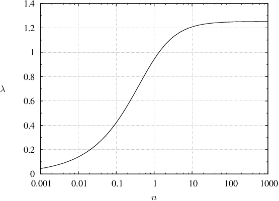
The non-dimensional factor

$$\lambda=\sqrt{\frac{\pi n}{2}}\frac{\Gamma(n+1)}{\Gamma\left(n+\frac{3}{2}\right)}$$ (20)

is shown in Fig. 1 as a function of polytropic index $n$. For reasonable values of $n\gtrsim\tfrac{1}{2}$ it is roughly of order one and becomes at most $\sqrt{\pi/2}$ in the isothermal limit (Lüst, 1952; Lynden-Bell, 1969).

Figure 1: The non-dimensional factor $\lambda$ as a function of polytropic index $n$.

A nice feature of the vertical structure equations given above is the possibility to compute the scale height of different contributions to the potential and combine them to one effective scale height:

$$h=\sqrt{\sum_{i}\frac{1}{h_{i}^{2}}}^{~-1}.$$

We demonstrate how to apply this to some important examples and compare the results to those given in the literature.

1. point mass $M_{\star}$:

   $$\Phi_{\ast}=\frac{G\,M_{\star}}{\sqrt{r^{2}+z^{2}}},\qquad\frac{\partial^{2}\Phi_{\ast}}{\partial z^{2}}\biggr|_{z=0}=\frac{G\,M_{\star}}{r^{3}}=\Omega_{\mathsf{K}}^{2}$$

   where $\Omega_{\mathsf{K}}$ is the Keplerian angular velocity. Hence the scale height of Keplerian discs is given by

   $$h=\frac{c_{\mathsf{s,c}}}{\Omega_{\mathsf{K}}}.$$ (21)

   This result has been known for decades in case of isothermal discs (Pringle, 1981, see, e.g. ) and was also obtained for polytropic discs by Hōshi (1977) and Paczynski (1978).

2. self-gravitating homogeneous slab:
   From Poisson’s equation we have (Mestel, 1963, see, e.g. )

   $$\frac{\partial^{2}\Phi}{\partial z^{2}}\biggl|_{z=0}=4\pi G\varrho_{\mathsf{c}}$$

   and therefore the scale height of the slab becomes

   $$h=c_{\mathsf{s,c}}\sqrt{4\pi G\varrho_{\mathsf{c}}}^{~-1}.$$ (22)

   The half-thickness computed from this result by use of Eq. (13) differs from that given in Paczynski (1978) for polytropic self-gravitating sheets. The deviation is of order one as long as $n$ is of order one and becomes large in the isothermal limit $n\to\infty$. However, in that case our solution reproduces exactly the result derived by Spitzer (1942).

3. point mass and self-gravitating homogeneous slab: Combining (i) and (ii) as described above leads to the result proposed by Lüst (1952) (Sakimoto & Coroniti, 1981, see also) who derived the scale height for self-gravitating isothermal sheets with central point mass:

   $$h=c_{\mathsf{s,c}}\sqrt{4\pi G\varrho_{\mathsf{c}}+\Omega_{\mathsf{K}}^{2}}^{~-1}.$$ (23)

   Thus again our more general result is consistent with the isothermal limit.

4. self-gravitating axisymmetric disc within an axisymmetric external potential $\Phi_{\mathsf{ext}}$ in radial balance:

   $$h=c_{\mathsf{s,c}}\Bigl(4\pi G\varrho_{\mathsf{c}}-2\Omega^{2}(1+x)+\Delta_{rz}\Phi_{\mathsf{ext}}\bigl|_{z=0}\Bigr)^{-\frac{1}{2}}$$ (24)

   where $x$ is the logarithmic derivative of midplane angular velocity $\Omega$ with respect to $r$

   $$x=\frac{\partial\ln\Omega}{\partial\ln r}.$$ (25)

   and $\Delta_{rz}$ is the axisymmetric Laplacian. The derivation uses again Poisson’s equation for the disc potential and in addition the gravitational balance law (Eq. 28). This result has been derived by Bertin & Lodato (1999) for isothermal discs. The contribution due to the external potential vanishes for all $r>0$ if $\Phi_{\mathsf{ext}}$ is the point mass potential. In that case the non self-gravitating limit ($\varrho_{\mathsf{c}}\to 0,x\to-\tfrac{3}{2}$) approaches the Keplerian value of the scale height. Another interesting case is Mestel’s disc (Mestel, 1963, see) which has $x=-1$ and the scale height becomes that of an infinite slab (22).

2.2 The slow accretion limit

In this section we will introduce the slow accretion limit (Lüst, 1952) and show that the transport equation for radial momentum (Eq. 5) simplifies to a balance law equating centrifugal and gravitational forces. Thereby we make use of some relations already derived in Sec. 2.1. The basis for the derivation shown below is the assumption that the rotational velocity of geometrically thin discs is highly supersonic and that the radial drift velocity is subsonic, i.e. $v_{r}\leq c_{\mathsf{s,c}}\ll v_{\varphi}$ (Pringle, 1981, see, e.g. ). In case of non self-gravitating discs the requirement of supersonic rotation is quite obvious and a direct consequence of the thin disc assumption. With help of Eq. (21) one concludes

$$1\ll\frac{r}{h}=\frac{r\Omega}{c_{\mathsf{s,c}}}=\frac{v_{\varphi}}{c_{\mathsf{s,c}}}.$$ (26)

We cannot derive a similar estimate if we take self-gravity into account, because in that case the scale height depends on mass distribution which in turn influences the rotational velocity. This makes the relation between $h$ and $v_{\varphi}$ more difficult. However, we will show in Section 2.4 that our approximations are at least consistent with the assumption given above.

With help of the vertical structure equation (17) we can eliminate $\Pi$ from the radial momentum equation (5). After multiplication with $r/c_{\mathsf{s,c}}^{2}$ one obtains

$$\begin{split}\frac{r}{c_{\mathsf{s,c}}^{2}}\frac{\partial v_{r}}{\partial t}+\biggl(\frac{v_{r}}{c_{\mathsf{s,c}}}\biggr)^{2}\frac{\partial\ln v_{r}}{\partial\ln r}=\biggl(\frac{v_{\varphi}}{c_{\mathsf{s,c}}}\biggr)^{2}-\frac{r}{c_{\mathsf{s,c}}^{2}}\frac{\partial\Phi}{\partial r}\\ -\eta\biggl\{\frac{\tfrac{3}{2}}{n+\tfrac{3}{2}}\frac{\partial\ln n}{\partial\ln r}+\frac{\partial\ln c_{\mathsf{s,c}}^{2}}{\partial\ln r}+\frac{\partial\ln\Sigma}{\partial\ln r}\biggr\}.\end{split}$$ (27)

Thereby we used Eq. (18) to express the logarithmic derivative of $\eta$ in terms of the logarithmic derivative of the polytropic index $n$. We can henceforth conclude that if the radial gradients of $n$, $c_{\mathsf{s,c}}$ and $\Sigma$ are moderate, i.e. their logarithmic derivatives are at most of order one, we can neglect the terms within the curly brackets multiplied by $\eta\leq 1$ in Eq. (27) in comparison with the term $(v_{\varphi}/c_{\mathsf{s,c}})^{2}\gg 1$. The same argument applies to the second term on the left hand side, which is also of order one as long as the radial drift velocity is subsonic. The remaining terms of the radial momentum equation are

$$r\frac{\partial v_{r}}{\partial t}=v_{\varphi}^{2}-r\frac{\partial\Phi}{\partial r}.$$

In the slow accretion limit one expects that temporal changes of the radial drift velocity $v_{r}$ occur on the viscous time-scale $\tau_{\mathsf{vis}}\gg\tau_{\mathsf{dyn}}\approx\Omega^{-1}=r/v_{\varphi}$. Hence we may approximate the term on the left hand side by

$$r\frac{\partial v_{r}}{\partial t}\approx r\frac{v_{r}}{\tau_{\mathsf{vis}}}=v_{r}v_{\varphi}\frac{\tau_{\mathsf{dyn}}}{\tau_{\mathsf{vis}}}\ll v_{\varphi}^{2}$$

and the radial momentum transport equation reduces to the gravitational balance law

$$v_{\varphi}^{2}=r\frac{\partial\Phi}{\partial r}.$$ (28)

This result has been known for decades since the early works of Weizsäcker (1948) and Lüst (1952). However, to our knowledge it has never been derived in such a general way using the vertical structure equations to rewrite the radial pressure gradient. By doing so we can explicitly show that radial pressure forces in geometrically thin discs are usually rather small compared to centrifugal and gravitational forces.

2.3 Monopole approximation and self-gravity

So far we did not point out how to compute the radial gravitational acceleration $-\frac{\partial\Phi}{\partial r}$. In general there would be contributions from the central object and the mass distribution within the disc. Thus it would involve the solution of Poisson’s equation which is difficult even in case of rotationally symmetric and geometrically thin systems. In this section we will introduce the monopole approximation for such systems and derive an approximate solution to Eq. (28).

The derivation basically follows the method of Toomre (1963) who uses Hankel transforms to compute the potential of razor-thin discs given in the equatorial plane by

$$\Phi_{\mathrm{d}}(r)=-2\pi G\int\limits_{0}^{\infty}\mathsf{d}kJ_{0}(kr)\int\limits_{0}^{\infty}\Sigma(s)J_{0}(ks)s\mathsf{d}s.$$ (29)

Here $J_{0}$ denotes the Bessel function of the first kind of order $0$. At about the same time Mestel (1963) found that the radial gravitational acceleration $-\frac{\partial\Phi}{\partial r}$ at a certain distance from the centre $r$ can be split up into three parts: The monopole term which depends on the enclosed mass (see Eq. 31) and contributions from the mass within and beyond $r$ (Mineshige & Umemura, 1997, see also). This solution involves spatial integrals over the mass distribution $\Sigma(r)$ which cannot be evaluated analytically in general.

However for certain centrally condensed mass distributions the monopole term is dominant and the two other terms cancel out as was already pointed out by Mestel (1963). Hence one may neglect all terms except for the monopole term and approximate the solution to Eq. (28) by

$$v_{\varphi}^{2}=\frac{GM(r)}{r}$$ (30)

with the enclosed mass

$$M(r)=M_{\star}+2\pi\int_{0}^{r}\Sigma(s)s\mathsf{d}s$$ (31)

where $M_{\star}$ is the mass of the central object. Since the error introduced by neglecting the two additional contributions depends on $\Sigma(r)$ it is difficult to estimate it in general.

In order to elucidate this we show how to derive Eq. (30) from Eq. (29). Unlike Mestel (1963) and Mineshige & Umemura (1997) we do not split up the gravitational acceleration obtained from (29) via differentiation. Instead we take the solution (29) add the potential of the central point mass and insert it into Eq. (28). Then we apply the inverse Hankel transform which provides us with an integral expression of the surface density (Binney & Tremaine, 1987, see)

$$\Sigma(r)=\frac{1}{2\pi G}\int\limits_{0}^{\infty}\mathsf{d}kJ_{0}(kr)\int\limits_{0}^{\infty}\biggl(v_{\varphi}(s)^{2}-\frac{GM_{\star}}{s}\biggr)kJ_{1}(ks)\mathsf{d}s.$$

If we insert this result in Eq. (31), we can compute the enclosed mass. Thereby the contribution due to the central point mass within the integral cancels the constant term $M_{\star}$. Thus we proceed utilizing integration by parts with respect to $s$ considering that

$$\frac{\partial}{\partial s}\Bigl(J_{0}(ks)\Bigr)=-kJ_{1}(ks)$$

which gives us

$$\begin{split}M(r)=\frac{r}{G}\biggl\{\int\limits_{0}^{\infty}\frac{\partial v_{\varphi}^{2}}{\partial s}\mathcal{F}(r,s)\mathsf{d}s-\Bigl[v_{\varphi}(s)^{2}\mathcal{F}(r,s)\Bigr]_{s=0}^{s=\infty}\biggr\}\end{split}$$

with

$$\mathcal{F}(r,s)=\int\limits_{0}^{\infty}\frac{1}{k}J_{1}(kr)J_{0}(ks)\mathsf{d}k=\begin{cases}\mathcal{F}_{<}(\tfrac{s}{r})\ \mathrm{if}\ s\leq r\\ \mathcal{F}_{>}(\tfrac{r}{s})\ \mathrm{if}\ s>r\\ \end{cases}.$$ (32)

The solution of this definite integral depends on whether $r<s$ or not. An analytical expression in terms of complete elliptic integrals is given in App. A together with asymptotic expansions which allow us to evaluate the surface terms. We may now split the integral into an inner $s<r$ and outer $s>r$ part

$$\begin{split}\frac{GM(r)}{r}&=\ v_{\varphi}(0)^{2}-\tfrac{1}{2}\lim_{s\to\infty}\tfrac{r}{s}v_{\varphi}(s)^{2}\\ &+\int\limits_{0}^{r}\frac{\partial v_{\varphi}^{2}}{\partial s}\mathcal{F}_{<}\bigl(\tfrac{s}{r}\bigr)\mathsf{d}s+\int\limits_{r}^{\infty}\frac{\partial v_{\varphi}^{2}}{\partial s}\mathcal{F}_{>}\bigl(\tfrac{r}{s}\bigr)\mathsf{d}s\end{split}$$

and substitute the variable of integration

$$\begin{split}&\frac{GM(r)}{r}=\ v_{\varphi}(0)^{2}-\tfrac{1}{2}\lim_{s\to\infty}\tfrac{r}{s}v_{\varphi}(s)^{2}\\ &+\int\limits_{0}^{1}\frac{\partial}{\partial k}\Bigl(v_{\varphi}(rk)\Bigr)^{2}\mathcal{F}_{<}(k)\mathsf{d}k-\int\limits_{0}^{1}\frac{\partial}{\partial k}\Bigl(v_{\varphi}(\tfrac{r}{k})\Bigr)^{2}\mathcal{F}_{>}(k)\mathsf{d}k.\end{split}$$

If we add $0=+1-1$ to the function $\mathcal{F}_{<}(k)$ in the first integral, carry out one integration and factor out the term $v_{\varphi}(r)^{2}$ we finally get the result

$$\begin{split}&\frac{GM(r)}{r}=\ v_{\varphi}(r)^{2}\Biggl\{1-\tfrac{1}{2}\lim_{s\to\infty}\frac{r}{s}\biggl(\frac{v_{\varphi}(s)}{v_{\varphi}(r)}\biggr)^{2}\\ &-\int\limits_{0}^{1}\mathcal{H}(r,kr)\frac{1-\mathcal{F}_{<}(k)}{k}\mathsf{d}k+\int\limits_{0}^{1}\mathcal{H}\bigl(r,\tfrac{r}{k}\bigr)\frac{\mathcal{F}_{>}(k)}{k}\mathsf{d}k\Biggr\}\end{split}$$ (33)

with

$$\mathcal{H}(r,s)=\frac{v_{\varphi}(s)^{2}}{v_{\varphi}(r)^{2}}\,\frac{\mathsf{d}\ln v_{\varphi}^{2}}{\mathsf{d}\ln s\ }=2\frac{s^{2}\Omega(s)^{2}}{r^{2}\Omega(r)^{2}}\biggl(\frac{\mathsf{d}\ln\Omega}{\mathsf{d}\ln s\ }+1\biggr)$$ (34)

The comparison with Eq. (30) reveals that the exact solution of the thin disc Poisson problem reduces to the monopole approximation if the sum in the curly brackets of Eq. (33) is close to one. This sum only depends on the rotation law given by $\Omega$ as a function of radial distance to the origin. Thus we may ask ourselves if there exist certain rotation laws for which this condition is fulfilled.

First of all one should restrict the discussion to rotation laws for which the centrifugal acceleration $r\Omega^{2}$ tends to zero at infinity. Thus $\Omega\propto r^{\kappa}$ with $\kappa<-\tfrac{1}{2}$ must hold in the limit $r\to\infty$. Then we can neglect the surface term and the deviation from the monopole approximation is completely determined by the two definite integrals which depend on the rotation law through $\mathcal{H}$ multiplied by the two weight functions $(1-\mathcal{F}_{<})/k$ and $\mathcal{F}_{>}/k$. These functions are both positive and smaller than one over the whole interval of integration (see Fig. 15 in the Appendix). Hence if $\mathcal{H}$ does not change its sign, i.e. $\Omega$ is monotone, both integrals may at least partly cancel each other.

The simplest monotone function one could think of as reasonable rotation law is a power law $\Omega\propto r^{\kappa}$. In this case one easily computes for (34)

$$\mathcal{H}_{\kappa}(r,s)=2(\kappa+1)\biggl(\frac{s}{r}\biggr)^{2(\kappa+1)}.$$

If we insert this into Eq. (33) the explicit dependence on $r$ is removed from the integrals. We can evaluate them numerically if we specify the power law exponent $\kappa$ of the rotation law. Hence the whole term within the curly brackets depends only on $\kappa$. This implies that $M\propto r^{2\kappa+3}$ and because $M(r)$ must be a monotonically increasing function of radius $\kappa\geq-\frac{3}{2}$ is required.

Figure 2: Deviation from monopole approximation for power law rotation curve $\Omega\propto r^{\kappa}$ as a function of the exponent.

In Fig. 2 the gravitational acceleration due to the monopole term divided by the centrifugal acceleration is shown as a function of $\kappa$. There are two cases where the monopole approximation is exact: $\kappa=-\frac{3}{2}$ and $\kappa=-1$. The former corresponds to Keplerian rotation whereas the latter is known as Mestel’s disc (Mestel, 1963, see). The error introduced by the monopole approximation would be less than $10\,\%$ for $-\frac{3}{2}<\kappa<-1$ and yet for $\kappa=-\frac{3}{4}$ one overestimates the gravitational acceleration acting inwards by less than a factor of $2$. This observation supports the remark in Lin & Pringle (1990) that the monopole approximation is usually good to the $5\,\%$ level. However, as $\kappa$ approaches $-\frac{1}{2}$ the second integral in Eq. (33) diverges and the monopole approximation breaks down.

2.4 Supersonic rotation and self-gravity

In Section 2.2 we made an important assumption for our model, namely that the azimuthal flow in the disc is highly supersonic ($v_{\varphi}\gg c_{\mathsf{s,c}}$). We showed that this is a consequence of the thin disc assumption if self-gravity is negligible. Unfortunately it is not possible to generalize these considerations and simply apply them to self-gravitating discs, because $v_{\varphi}$ couples to the surface density which is not known a priori.

However, if the radial balance law (30) holds, we know something about the relation between matter distribution and rotation law. Hence we can at least check, if this relation is consistent with the assumption of supersonic rotation. The differentiation of Eq. (30) with respect to $r$ implies that

$$\frac{\partial M}{\partial r}=\frac{v_{\varphi}^{2}}{G}\left(2x+3\right)$$ (35)

where $x$ is the logarithmic gradient of the rotation law (Eq. 25). With the definition of the enclosed mass in Eq. (31) we can derive another expression of its radial gradient:

$$\frac{\partial M}{\partial r}=2\pi\,r\Sigma.$$ (36)

Hence, by equating the right hand side of Eqs. (35) and (36) we obtain:

$$2\pi G\Sigma=r\Omega^{2}\left(2x+3\right).$$ (37)

One can use this result together with Eq. (19) to eliminate $\varrho_{\mathsf{c}}$ from Eq. (24). If one furthermore substitutes point mass potential for external potential this finally becomes

$$\left(\frac{c_{\mathsf{s,c}}}{v_{\varphi}}\right)^{2}=\frac{1}{\lambda}\left(2x+3\right)\frac{h}{r}-2(x+1)\left(\frac{h}{r}\right)^{2}$$ (38)

where $\lambda$ is of order unity for reasonable values of the polytropic index $n$ (see Fig. 1). This expression is the generalization of Eq. (26) for geometrically thin self-gravitating discs in radial balance with gravitational acceleration given by the monopole approximation. It obviously simplifies to the non self-gravitating case in the limit $x\to-3/2$. However, if the disc is self-gravitating, the logarithmic derivative of $\Omega$ becomes larger than $-3/2$ and the term of order $h/r$ on the right hand side dominates and one gets $(c_{\mathsf{s,c}}/v_{\varphi})^{2}\propto h/r$. But none the less the relation $(c_{\mathsf{s,c}}/v_{\varphi})^{2}\ll 1$ still holds and hence gravitational balance and monopole approximation are at least consistent with the assumption of supersonic rotation in case of geometrically thin self-gravitating discs.

2.5 The disc evolution equation

In this section we will summarize the results obtained so far and derive the disc evolution equation. The basic equations of thin disc evolution were given in the introductory paragraph of Sec. 2. In the successive subsections we showed that one can replace the radial momentum transport equation (5) by Eq. (30) with the enclosed mass $M(r)$ defined by Eq. (31). Because of this it is convenient to replace the surface density in the continuity equation (4) by the enclosed mass as well and treat it as a time-dependent function too. Hence the radial integration of (4) yields

$$\frac{\partial M}{\partial t}=-2\pi\,r\Sigma v_{r}.$$ (39)

With help of Eq. (36) we may eliminate $\Sigma$ (Weizsäcker, 1948):

$$\frac{\partial M}{\partial t}+v_{r}\frac{\partial M}{\partial r}=0.$$ (40)

This replaces the continuity equation (4) in the set of model equations.

We proceed by transforming the angular momentum transport equation (6). Because of Eq. (40) we can eliminate $v_{r}$ with the quotient of temporal and radial derivatives of $M$ and with help of the balance law (30) we may replace $M$ by $rv_{\varphi}^{2}/G$ in these derivatives. Thus the left hand side of Eq. (6) becomes

$$\frac{\partial\ell}{\partial t}+v_{r}\frac{\partial\ell}{\partial r}=-\biggl(\frac{\partial\ln M}{\partial\ln r}\biggr)^{-1}\frac{\partial\ell}{\partial t}=-\frac{M}{2\pi\Sigma}\frac{\partial\Omega}{\partial t}.$$

In the last step we used Eq. (36) and $\ell=r^{2}\Omega$. If we multiply the angular momentum equation (6) by $2\pi r\Sigma$ and use the result above on the left hand side it transforms to

$$-rM\frac{\partial\Omega}{\partial t}=\frac{\partial}{\partial r}\Bigl(2\pi r^{2}T_{r\phi}\Bigr)=\frac{\partial}{\partial r}\Bigl(\nu 2\pi r\Sigma r^{2}\partial_{r}\Omega\Bigr)$$

with the viscous stress tensor component given in (3). Again we can replace $M$ by utilizing Eq. (30) and $\Sigma$ with help of Eq. (37). Thus the final result for the disc evolution equation becomes

$$-r^{4}\Omega^{2}\frac{\partial\Omega}{\partial t}=\frac{\partial}{\partial r}\Bigl(\nu\,r^{3}\Omega^{3}x\bigl(2x+3\bigr)\Bigr).$$ (41)

Equation (41) together with the local power law exponent $x$ defined in (25) is a non-linear second order partial differential equation which describes the advection and diffusion of angular velocity under the influence of self-gravity and viscous friction.

If the kinematic viscosity $\nu(r,t)$ is given as a function of radial distance and time, one may in principle derive a solution to the disc equation provided that one specifies appropriate initial and boundary conditions. Even if $\nu$ is not given explicitly, the equation remains solvable if the viscosity depends on $\Omega$ directly or indirectly through $\Sigma$ or $M$. We will discuss some possibilities for an appropriate viscosity prescription applicable to accretion discs in the next section.

The disc evolution equation derived by Trefftz (1952) seems to be quite similar compared to our equation. However, we would like to emphasize that there exists a very important difference. In contrast to our approach Trefftz (1952) solves Poisson’s equation for the disc potential in a pure two-dimensional world. Therefore she obtains $M\propto v_{\varphi}^{2}$ as the radial balance law. This result differs considerably from the solution we yield for an infinitesimally thin disc embedded in a three-dimensional space.

2.6 Viscosity prescription

A proper description of the viscosity coefficient $\nu$ is a perennial problem when modelling accretion discs. Although there has been a long lasting debate since the early works of Weizsäcker (1948) and Lüst (1952) on the nature of the viscosity coefficient it became a broad consensus that molecular viscosity is not sufficient to explain the accretion process (Frank et al., 2002). In case of non self-gravitating discs there are basically two processes that lead to sufficiently high stresses: Strong, large scale magnetic fields and turbulence (Shakura & Sunyaev, 1973).

However, in self-gravitating discs there exists a completely different mechanism for redistribution of angular momentum. If these discs become gravitationally unstable, they can transfer angular momentum via compressible density waves and dissipate energy in shocks (Balbus & Papaloizou, 1999). Since the amount of angular momentum transfer depends on the details of the inhomogeneous structures, one usually has to perform multidimensional simulations to investigate these processes. Thus it has been the fundamental question of self-gravitating accretion disc theory in the past 20 years whether or not it is possible to model those discs with a simple one-dimensional diffusion model. Since we do not want to repeat ourselves we refer to Sec. 1 for a short review of the most important findings including important references. We proceed summarizing the discussion on this issue with the statement that the viscous diffusion approximation seems possible even for self-gravitating discs if they are geometrically thin and not too massive.

In the context of non self-gravitating discs a very popular description of the effective shear stresses was proposed by Shakura & Sunyaev (1973) who derived a parametrization which couples the dominant stress tensor component $t_{r\varphi}$ to pressure

$$t_{r\varphi}=-\alpha P$$ (42)

with model parameter $0<\alpha<1$. If we carry out vertical integration according to Eqs. (2) and (3), we can cast this equation with help of Eq. (17) into an expression for the effective turbulent viscosity (Lin & Pringle, 1990, see)

$$\nu=\tilde{\alpha}\frac{c_{\mathsf{s,c}}^{2}}{\Omega}.$$ (43)

The new parameter $\tilde{\alpha}=-\alpha\eta/x$ is again smaller than one, because $\eta\leq 1$ (see Eq. (18)) and the logarithmic derivative of $\Omega$ (Eq. 25) is negative and of order one. Balbus & Hawley (1991) have discussed an instability that in magnetic accretion discs can give rise to viscous stresses of the $\alpha$ type with – if only marginally – the required strength.

The $\alpha$ viscosity couples to the midplane speed of sound $c_{\mathsf{s,c}}$ which in turn depends on midplane temperature. Therefore it is generally not possible to compute the viscosity coefficient without knowing anything about the temperature distribution within the disc. Unfortunately this would require solving the energy equation in addition to the disc evolution equation derived in the previous section. Paczynski (1978) was the first who came up with the idea of self-regulation (Bertin, 1997; Bertin & Lodato, 1999; Lodato, 2007, see also) which circumvents the solution of the energy equation by simply proposing that the flow in self-gravitating discs is always at the border of instability $Q\approx 1$ with the Toomre parameter (Toomre, 1964, see)

$$Q=\frac{c_{\mathsf{s,c}}{\color[rgb]{0,0,0}\kappa_{\mathrm{e}}}}{\pi G\Sigma}\approx\frac{c_{\mathsf{s,c}}\Omega}{\pi G\Sigma}$$ (44)

where ${\color[rgb]{0,0,0}\kappa_{\mathrm{e}}}$ is the epicyclic frequency

$${\color[rgb]{0,0,0}\kappa_{\mathrm{e}}}=\Omega\sqrt{\frac{\partial\ln\ell^{2}}{\partial\ln r}}=\Omega\sqrt{2x+4}\approx\Omega.$$

The error induced by the approximation is of order unity for any reasonable value of $x$. If we solve Eq. (44) for $\Sigma$ and insert the result into Eq. (37) we obtain an expression for $c_{\mathsf{s,c}}$ in terms of $v_{\varphi}$ and $Q$:

$$c_{\mathsf{s,c}}=\left(x+\tfrac{3}{2}\right)Qv_{\varphi}$$ (45)

which allows us to eliminate $c_{\mathsf{s,c}}$ from the viscosity prescription (43). Hence we finally get

$$\nu=\tilde{\beta}(2x+3)^{2}r^{2}\Omega$$ (46)

with the new parameter $\tilde{\beta}=\tilde{\alpha}Q^{2}/4$. We would like to mention that the assumption of marginal stability, i.e. $Q\approx 1$, might be a problem, because this would contradict the assumption of supersonic motion for self-gravitating discs where the logarithmic derivative of the rotation law deviates from its Keplerian value $x=-3/2$ (see Eq. (45) and discussion in Sec. 2.4). The viscosity prescription in Eq. (46) was first proposed by Lin & Pringle (1987, hereafter LP) who assumed that the turbulent viscosity is caused by some kind of gravitational instability:

$$\nu=L_{\mathrm{crit}}^{2}\Omega=\biggl(\frac{G\Sigma}{\Omega^{2}}\biggr)^{2}\Omega$$

where $L_{\mathrm{crit}}$ is the typical length scale of unstable modes. If we eliminate $\Sigma$ using Eq. (37) we can transform this equation into

$$\nu=\biggl(\frac{2x+3}{2\pi}\biggr)^{2}r^{2}\Omega$$

which becomes exactly (46) if we set $\tilde{\beta}=1/4\pi^{2}\approx 0.025$. It was already mentioned by Bertin & Lodato (1999) and others (Lin & Pringle, 1990, see) that LP viscosity prescription fails inevitably in the Keplerian limit, because self-regulation can only occur in the self-gravitating regime where the disc can become gravitationally unstable. The consequence is that $\nu$ vanishes as $x\to-3/2$. The reason for this odd behaviour is the assumption that one can assign a finite and fixed value to $Q$ and therefore $\tilde{\beta}$. However, in the Keplerian limit the disc must be Toomre stable and therefore $Q$ must become much larger the one. This could compensate the factor $(2x+3)^{2}$ in the viscosity prescription which tends to zero as $x\to-3/2$. To shed more light on this, we insert the ratio $c_{\mathsf{s,c}}/v_{\varphi}$ from Eq. (45) into Eq. (38). If we assume that the ratio $h/r$ is small, but always larger than zero in the Keplerian limit as $x\to-3/2$, we conclude that the left hand side of

$$\left(x+\tfrac{3}{2}\right)^{2}Q^{2}=\left(2x+3\right)\frac{h}{r}-2(x+1)\left(\frac{h}{r}\right)^{2}$$

must remain greater than zero too and therefore the viscosity should not vanish if self-gravity becomes negligible. However it might become rather small, because $h/r\ll 1$ in thin discs.

The simplest modification of (46) to overcome these limitations would be to assume that $\nu\propto r^{2}\Omega$. A viscosity of this kind was proposed by Duschl et al. (1998, , hereafter DSB) who assumed that the effective Reynolds number does not fall below the critical Reynolds number. The so-called $\beta$-ansatz just reads

$$\nu=\beta\,rv_{\varphi}=\beta\,r^{2}\Omega.$$ (47)

where the constant parameter $\beta$ is given by the inverse of the critical Reynolds number. This is still a parameterization and not an ab-initio solution to the problem. The ansatz (47), however, has several promising aspects:

1. For fully self-gravitating disk regions, which are dominated by the mass distribution of the disk in the direction perpendicular to the rotational plane as well as in the rotational plane itself, ansatz (47) is equivalent to the hypothesis that the ratio of dynamic timescale ($\tau_{\mathrm{dyn}}\sim\Omega^{-1}$) and viscous timescale ($\tau_{\mathrm{vis}}\sim r^{2}/\nu$) is constant. In other words one assumes a linear relation between the two relevant timescales: $\tau_{\mathrm{vis}}=\beta^{-1}\tau_{\mathrm{dyn}}$. Duschl & Britsch (2006) succeed in showing numerically that instabilities in a self-gravitating flow lead to a viscosity of the functional form of the $\beta$-ansatz, indeed. This is furthermore supported by the observation that in the fully self-gravitating limit, where the rotation law deviates considerably from Keplerian motion ($x>-3/2$), the $\beta$-prescription approaches the values obtained with the self-regulated $\alpha$-ansatz. (46).

2. For Keperian self-gravitating disk regions, the vertical structure is dominated by local self-gravity, i.e. , the local mass distribution in the disk, while in the rotational plane the (almost) equilibrium between gravitational and centrifugal forces is still determined by the central mass, i.e. , the rotational velocity is Keplerian. There a functional form of (47) solves the problem of a quasi-thermostat as discussed by Duschl et al. (2000).

3. In the limit of negligible self-gravity (Keplerian disk regions) it smoothly merges into the $\alpha$-prescription (Duschl et al., 1998; Duschl et al., 2000). This can be seen by plugging the non-self-gravitating (Keplerian) scale-height (21) in the $\beta$-viscosity prescription (47):

   $$\nu=\beta\frac{v_{\varphi}^{2}}{\Omega}=\beta\left(\frac{r}{h}\right)^{2}\frac{c_{\mathsf{s,c}}^{2}}{\Omega}.$$

   A comparison with the $\alpha$-ansatz (Eq. 43) reveals the above mentioned relation. Here, $\beta$ is equivalent to a constant Reynolds number.

In that respect the $\beta$-ansatz is, at least formally, a generalization of the classical $\alpha$-ansatz, which otherwise runs into trouble in the fully and Keplerian self-gravitating domains. To couple all three regions, $\beta$ needs to be chosen such that a smooth transition between them can be achieved. If, similar to the reasoning for classical accretion disks, one takes resort to time scale arguments, it turns out that the standard values of $\alpha$, which are of the order of $10^{-2\dots 0}$, are compatible with values of $\beta$ which correspond to those of the inverse of the critical Reynolds number. Some aspects of this have also been investigated by Richard & Zahn (1999, hereafter RZ) who proposed a quite similar prescription:

$$\nu=\beta\,r^{3}\biggl|\frac{\partial\Omega}{\partial r}\biggr|=\beta\,\left|x\right|\,r^{2}\Omega.$$ (48)

It differs from the previous one by a factor of $|x|$ which is of order unity in most cases.

All the parametrizations described above differ only in their dependence on the local power law exponent $x$. Hence we may combine the three viscosity functions into one formula and introduce a new function $f(x)$ to distinguish between these prescriptions

$$\nu=\beta r^{2}\Omega f(x)\quad\textnormal{with}\quad f(x)=\begin{cases}1&\textnormal{DSB}\\ |x|&\textnormal{RZ}\\ (2x+3)^{2}&\textnormal{LP}\end{cases}$$ (49)

The magnitude of the viscous coupling constant $\beta$ proposed by LP and DSB is of order $10^{-2}$ to $10^{-3}$ whereas RZ derived smaller values of approximately $4\cdot 10^{-6}$. However, the precise value of $\beta$ is not of substantial importance for the solution of the disc evolution equation. If we define the new time variable $\tau=\beta\,t$ we can rewrite Eq. (41) thereby eliminating $\beta$ from the equation

$$-r^{4}\Omega^{2}\frac{\partial\Omega}{\partial\tau}=\frac{\partial}{\partial r}\Bigl(r^{5}\Omega^{4}x(2x+3)f(x)\Bigr).$$ (50)

Hence we can transform any solution $\Omega(r,\tau)$ back to $\Omega(r,t)$ by rescaling the time variable. Although Eq. (50) does not depend on $\beta$, its actual value may have an impact on the solution due to boundary conditions (see Sec. 3.3.2).

3 Self-similar solutions

In this section we show how to solve Eq. (50) using similarity methods. To simplify the derivation we introduce non-dimensional variables and functions and rewrite the disc evolution equation in terms of these. If we specify an arbitrary length scale $\tilde{r}$ and mass scale $\widetilde{M}$ and define the time scale $\tilde{\tau}$ according to

$$\tilde{\tau}=\sqrt{\frac{\tilde{r}^{3}}{G\,\widetilde{M}}}$$ (51)

we can non-dimensionalize all variables, functions and equations derived in the previous sections. The equations retain their form except for those containing Newton’s gravitational constant $G$ which must be set to unity in the non-dimensional equations. Once we have solved the self-gravitating accretion disc problem for the non-dimensional functions we can use these scaling parameters to switch back to the real world quantities. In Sec. 4.5 we discuss the self-similar evolution of massive AGN accretion discs and demonstrate how to apply the inverse transformations to recover the dimensioned quantities.

3.1 Differential equation of self-similar evolution

A short calculation yields that Eq. (50) is invariant under the family of one-parameter Lie groups of scaling transformations

$$r^{\prime}=\lambda^{a}r,\qquad\tau^{\prime}=\lambda^{b}\tau,\qquad\Omega^{\prime}=\lambda^{c}\Omega$$ (52)

if and only if $c=-b$. The group invariants are

$$\xi=r\tau^{1/\kappa}\quad\textnormal{and}\quad y=-(\kappa\Omega\tau)^{-1}$$ (53)

with $\kappa=-b/a$ the general group invariant solution is determined by the expression $F(y,\xi)=0$ where $F$ is a (not yet determined) function of the group invariants. This is an implicit definition of the function $y(\xi)$. Thus with Eq. (53) one can write down the explicit form of the group invariant solutions

$$\Omega(r,\tau)=-\frac{1}{\kappa\tau\,y\bigl(\xi(r,\tau)\bigr)}.$$ (54)

The remaining problem is to determine $y$ as a function of the similarity variable $\xi$.

If we apply the original PDE (50) with $x$ given by Eq. (25) to the group invariant solutions we obtain a coupled system of ordinary differential equations (ODEs) for $x(\xi)$ and $y(\xi)$

$$\frac{\mathsf{d}x}{\mathsf{d}\ln\xi} =\frac{(x-\kappa)y-(4x+5)z(x)}{z^{\prime}(x)}$$ (55)

$$\frac{\mathsf{d}y}{\mathsf{d}\ln\xi} =-xy$$ (56)

where $z^{\prime}(x)$ is the derivative with respect to $x$ of the viscosity dependent function

$$z(x)=x(2x+3)f(x)=\begin{cases}x(2x+3)&\textnormal{DSB}\\ -x^{2}(2x+3)&\textnormal{RZ}\\ x(2x+3)^{3}&\textnormal{LP}\end{cases}$$ (57)

and $f(x)$ is given by Eq. (49). In case of the RZ-prescription we assumed that $x<0$, i.e. $\Omega$ always decreases as $r\to\infty$. The remaining constant $\kappa$ in Eq. (55) is a free parameter which has to be determined from the auxiliary conditions (see Section 3.2).

The planar differential system (55,56) is an autonomous set of two first order ODEs. It is always possible to reduce these systems by elimination of the independent variable to a single first order equation

$$\frac{\mathsf{d}x}{\mathsf{d}y}=\frac{(4x+5)z(x)-(x-\kappa)y}{xz^{\prime}(x)y}.$$ (58)

The solution of Eq. (58) gives $x(y)$ which can be used to integrate Eq. (56)

$$\ln\xi=-\int\frac{\mathsf{d}y}{x(y)y}.$$ (59)

This yields $\xi(y)$ and its inverse $y(\xi)$ which is required to compute the self-similar solution $\Omega(r,\tau)$ given in Eq. (54). Unfortunately, Eq. (58) is a non-linear ODE and one cannot expect to solve it in terms of known functions, in general. In fact, the inverse of Eq. (58) is an Abel Equation of the second kind. We were not able to identify a non-linear transformation which maps our equation to any of the few classes with known analytical solutions (Polyanin & Zaitsev, 2003, see, e.g. ).

Although analytical solutions are not excluded per se, we focused on numerical methods to solve the self-similar disc equations. The task is basically to solve the autonomous system of ODEs (55,56) which can be achieved using standard techniques. However, the system under investigation exhibits some pitfalls such as singular points where the solution is not unique. Careful treatment of these peculiarities is essential. We discuss the numerical solution procedure in detail in Sec. 3.3.

3.2 Auxiliary conditions

The problem addressed in the previous sections is a so-called initial-boundary-value problem. This problem is well defined only if we provide auxiliary conditions in addition to the PDE (50) describing the dynamical evolution of the function $\Omega(r,\tau)$. Thus we have to define some initial state $\Omega_{0}(r)$ at time $\tau=0$ from which the solution evolves and we must specify how $\Omega$ changes on the boundary of the spatial domain for all $\tau>0$. Since the spatial domain we are interested in is the positive real axis, its boundary is determined by the limits $r=0$ and $r\to\infty$. Therefore one has to specify three auxiliary conditions.

If we are looking for self-similar solutions, we demand an additional restriction to the set of possible solutions which must be related to the auxiliary conditions. The self-similar solutions are obtained from the integration of the first order system of ODEs (55, 56). In contrast to the original PDE, this problem is well posed if we supply initial conditions for $x$ and $y$. Hence the number of necessary auxiliary conditions is reduced by one. As a consequence self-similar solutions only exist if two of the original conditions coalesce (see Ames, 1965, Chap. 4.3). Thus, although one can normally choose arbitrary auxiliary conditions, the requirement of self-similarity imposes some restrictions (see Sec. 3.2.2).

In addition, one has to ensure that these conditions are consistent with the underlying physical model. In case of the disc evolution model described above there are some constraints due to the fact that the surface density $\Sigma$ must be positive everywhere at any time. The same applies to the enclosed mass which is not only positive but also a monotonically increasing function of radial distance $\partial_{r}M\geq 0$ for all $r>0$ (see Eq. (36)). Since $\Omega$ is related to $M$ via Eq. (30) the auxiliary conditions (and the solutions too) must fulfill

$$r^{3}\Omega^{2}>0\quad\Leftrightarrow\quad\Omega\neq 0$$ (60)

and

$$\frac{\partial\ln r^{3}\Omega^{2}}{\partial\ln r}=2x+3\geq 0\quad\Leftrightarrow\quad x\geq-\tfrac{3}{2}$$ (61)

for all $0<r<\infty$ and $0\leq\tau<\infty$. Condition (60) may become even more restrictive if we demand that $\Omega$ must be continuous. Therefore we conclude that

$$\Omega>0.$$ (62)

The sign is determined by the orientation of the rotational axis, which we define to point always in the positive $z$-direction.

3.2.1 Initial conditions

Let us suppose that the initial condition $\Omega_{0}(r)$ satisfies the relations (61, 62). With Eqs. (53) we obtain

$$\Omega_{0}(r)=-\lim_{\tau\to 0}\bigl(\kappa\tau y(\xi(r,\tau))\bigr)^{-1}=-\kappa r^{\kappa}\lim_{\xi\to\infty}\bigl(\xi^{\kappa}y(\xi)\bigr)^{-1}$$

where we assumed that $\kappa<0$ (which will be justified below). The limit on the right hand side is independent of $r$ and should be finite. Hence we conclude that

$$y(\xi)\propto\xi^{-\kappa}\quad\mathrm{as}\quad\xi\to\infty$$ (63)

which has the implication that the initial condition for self-similar solutions must be a power law of radius

$$\Omega_{0}(r)\propto r^{\kappa}.$$ (64)

In view of this result the assumption that $\kappa<0$ seems reasonable because otherwise the initial $\Omega_{0}$ would be an increasing function of radius which we want to exclude from our considerations (see Sec. 2.3). We therefore conclude that the so far unknown parameter $\kappa$ in Eq. (55) introduced by the requirement of group invariance imposed on the solution is simply the power law exponent of the initial condition.

We already discussed in Section 2.3 that rotation laws $\Omega\propto r^{\kappa}$ with an exponent $\kappa$ greater than $-\tfrac{1}{2}$ cause infinite centrifugal forces as $r\to\infty$. Furthermore we showed that the monopole approximation breaks down if the power law exponent approaches $-\tfrac{1}{2}$. Taking into account that Eq. (61) holds, one should therefore demand that

$$-\tfrac{3}{2}\leq\kappa\lesssim-\tfrac{3}{4}.$$ (65)

This restricts the parameter $\kappa$ to a very limited range of accessible values between centrally condensed mass distributions and configurations with flattened rotation curve where the mass is initially dispersed over the whole disc.

3.2.2 Boundary conditions

Normally one can think of a variety of physically meaningful boundary conditions for the self-gravitating accretion disc problem. However, in case of self-similar solutions the selection of valid boundary conditions is restricted, as was already mentioned above. Since $\xi$ depends on $r$ and $\tau$ according to (53) we have

$$\xi\to\infty\Leftrightarrow\begin{cases}\tau\to 0&\textnormal{for any fixed}\quad 0<r<\infty\\ r\to\infty&\textnormal{for any fixed}\quad 0<\tau<\infty\end{cases}$$

if $\kappa<0$. Therefore the outer boundary condition must coalesce with the initial condition.

This result becomes quite clear, if one remembers that the dynamic time scale for the discs evolution is roughly given by the inverse of $\Omega$. Since the initial condition is a decreasing power law, its inverse tends to infinity as $r$ approaches infinity. The evolutionary time scale becomes infinitely large which means that the disc does not evolve at all and stays in its initial state at the outer rim.

At the inner boundary there are basically two types of reasonable boundary conditions: Vanishing and finite torque supplied at the origin. The viscous torque $G(r,\tau)$ is given by

$$G(r,\tau)=2\pi r^{2}T_{r\varphi}$$ (66)

where the stress tensor component $T_{r\varphi}$ is defined in Eq. (3). One easily verifies that this could be rewritten in terms of $x(\xi)$, $y(\xi)$ and the similarity variable $\xi$:

$$G(r,\tau)=\beta\kappa^{-4}\,\tau^{-(5/\kappa+4)}~\xi^{5}\,y^{-4}\,z(x).$$ (67)

For any fixed and finite time $\tau$ Eq. (53) yields

$$\xi\to 0\Leftrightarrow r\to 0$$

We therefore conclude that the torque vanishes at the inner boundary at any time $0<\tau<\infty$ if

$$\lim\limits_{\xi\to 0}\xi^{5}\,y^{-4}\,z(x)=0.$$ (68)

An alternative would be that this limit is finite. In that case there are three distinct ways how the torque acts on the inner boundary depending on the value of $\kappa$, namely

$$\kappa<-\tfrac{5}{4}\qquad\textnormal{the torque decreases with time}$$

$$\kappa=-\tfrac{5}{4}\qquad\textnormal{the torque remains constant}$$

$$\kappa>-\tfrac{5}{4}\qquad\textnormal{the torque increases with time.}$$

Therefore a constant torque boundary condition is only applicable if the initial condition has a unique slope. We would like to emphasize that this restriction is due to the requirement of self-similarity imposed on the solutions and not a limitation of our disc model. However, one should not be worried too much, because in any realistic accretion disc scenario one would not expect that the torque acting at the inner boundary remains constant over a significant time span. In fact the most reasonable assumption in case of discs around black holes seems to be the zero torque boundary condition, because the event horizon prohibits any coupling to the central object. Another possibility would be a central object of finite size like an inner – possibly geometrically thick – accretion disc or a spinning protostar with spatial extent much smaller than the typical scales of the surrounding self-gravitating disc. In that case the torque acting at the inner boundary may indeed be finite and it is most likely that it decreases with time as the central object spins down.

3.2.3 Conservation conditions

Instead of the initial condition one could also specify the required auxiliary condition using a different but equivalent formulation. Let’s define

$$\mathcal{C}(\tau)=2\pi\int_{0}^{R(\tau)}\Sigma\Omega^{a}r^{b}r\mathsf{d}r$$

with arbitrary constant exponents $a$ and $b$. The quantity $\mathcal{C}$ is conserved if

$$\frac{\mathsf{d}\mathcal{C}}{\mathsf{d}\tau}=0.$$ (69)

For example if $a=0$ and $b=0$ then $\mathcal{C}$ is the enclosed mass within radial distance

$$R(\tau)=\xi_{0}\tau^{-1/\kappa}$$

where $\xi_{0}$ is a fixed value of the similarity variable $\xi$ (Eq. 53). We may rewrite the definition of $\mathcal{C}$ using non-dimensional variables and functions:

$$\mathcal{C}(\tau)=\frac{\int_{0}^{\xi_{0}}(2x+3)y^{-(a+2)}\xi^{b+2}\mathsf{d}\xi}{\kappa^{(a+2)}\tau^{(a+2)+(b+3)/\kappa}}$$ (70)

Since $\mathcal{C}$ must be finite in order to be conserved, the integral in the nominator should give a finite number and condition (69) is fulfilled if the exponent of $\tau$ in the denominator vanishes, i.e.

$$\kappa=-\frac{b+3}{a+2}.$$ (71)

The initial power law exponent $\kappa$ is completely determined by the numbers $a$ and $b$ which define the conserved quantity $\mathcal{C}$. Therefore one concludes that each initial condition generates a self-similar solution with specific conservation properties.

For example, if $a=0$ and $b=0$, $\mathcal{C}$ is the enclosed disc mass within radius $R(\tau)$ which is conserved if $\kappa=-\frac{3}{2}$. This is a reasonable result because in that case the mass of the disc must be finite and therefore the rotation law at the outer boundary as $r\to\infty$ is necessarily Keplerian. We will discuss these solutions in more detail in Sec. 4.2.

Another interesting case is $a=1$ and $b=2$ where $\mathcal{C}$ corresponds to the discs angular momentum. Unfortunately, this leads to $\kappa=-\tfrac{5}{3}$ which conflicts with the requirement in Eq. (65). Thus a physically meaningful self-similar solution with conserved angular momentum within the disc throughout the whole evolution does not exist. This does not mean that all other solutions violate angular momentum conservation. Instead, these discs do exactly what they are supposed to do, namely they transfer angular momentum from the inner regions to the environment beyond the radius $R(\tau)$.

3.3 Numerical method

As already mentioned in Section 3.1 the initial value problem defined by the system of non-linear ODEs (Eqs. 55 and 56) can be solved numerically with standard techniques. We use the programs ode (Tufillaro, Abbott & Reilly, 1992) and lsode (Hindmarsh, 1983) which implement different numerical integration schemes including explicit and semi-implicit methods such as Runge-Kutta-Fehlberg and predictor-corrector Adams-Moulton schemes as well as fully implicit schemes like Gear’s method which utilizes Backward Differentiation Formulas (BDF) (see Hairer, Nørsett & Wanner, 1993, and references therein).

For comparison we tried another numerical scheme which solves differential algebraic equations (DAE). Thereby we must transform the system of ODEs into a system of DAEs which was simply done by adding $z(\xi)$ to the set of independent functions. Then rewriting Eq. (55) yields a differential equation for $z(\xi)$ which must be combined with Eq. (56) and the algebraic constraint for $x(\xi)$ given by Eq. (57). As for ODEs there is a variety of different numerical methods available to solve DAEs (Hairer & Wanner, 1996; Petzold & Ascher, 1998, see). We used the program daspk described in Brown, Hindmarsh & Petzold (1994).

We found that the results obtained with the different programs and numerical schemes are similar within limits of numerical errors. In view of performance and numerical efficiency we would certainly recommend the BDF scheme and the DAE solver which allow for larger step sizes. This is important for large $\xi$ because the system becomes stiff in this limit.

Moreover, in order to solve the problem one has to determine feasible initial values for the numerical integration. This basically implies that the solutions obtained with these initial values must satisfy the restrictions and the auxiliary conditions discussed in the previous section. But there are still some free parameters, namely the proportionality constant in the initial condition (Eq. 64) and the torque applied to the disc at the inner boundary (Eq. 67).

3.3.1 Phase Plane

Figure 3: Phase diagram of the planar differential system defined by Eqs. (55,56) for DSB viscosity prescription with $\kappa=-6/5$. The arrows show the local gradient of the integral curves with direction pointing towards increasing values of the parameter $\xi$ on the curve. Some selected solutions obtained for different initial values are shown as solid curves.

In this section we examine the phase plane of the planar differential system to get an idea of the solutions topology. By doing so we can check which part of the parameter space is admitted by the restrictions given above. Since the differential equations depend on the parameter $\kappa$ and the viscosity prescription through the function $z(x)$ (Eq. 57) the phase diagram shown in Fig. 3 would change if these were varied. However, the main features remain unchanged. Among these are

• two nodes on the $x$-axis at $x=-\tfrac{3}{2}$ and $x=0$

• one saddle point on the $x$-axis at $x=-\tfrac{5}{4}$

• one singular vertical line.

The location of the singular line $x_{\mathsf{c}}$ depends on the viscosity prescription ($-\tfrac{3}{4}$ for DSB, $-1$ for RZ and $-\tfrac{3}{8}$ for LP). In addition, there exists another singular point – except for the case where $\kappa=x_{\mathsf{c}}$ – which is always located on the singular line. On the singular line the numerical integration fails, because the denominator on the right hand side of Eq. (55) vanishes which causes the derivative of $x$ with respect to $\ln\xi$ to become infinitely large as $x\to x_{\mathsf{c}}$. The only way a solution may continuously pass it, would be through the fourth singular point where the numerator vanishes simultaneously. The type of this singular point and its location on the singular line depends on viscosity prescription and $\kappa$:

$$\textnormal{DSB:}\,\frac{9}{4\kappa+3},\quad\textnormal{RZ:}\,\frac{1}{\kappa+1},\quad\textnormal{LP:}\,\frac{15309/128}{8\kappa+3}.$$

The point disappears (its $y$-value tends to infinity) in all cases if $\kappa$ equals the location of the singular line $x_{\mathsf{c}}$. It lies below the $x$-axis if $\kappa<x_{\mathsf{c}}$ and otherwise above it.

In Fig. 3 the shaded area marks the region where the solutions match the requirements (61) and (62). In addition we set an upper limit on $x$ to exclude rather flat rotation curves where the monopole approximation no longer holds (see Sec. 2.3). There are basically two distinct families of integral curves of interest. One starts somewhere on the singular line $x_{\mathsf{c}}>\kappa$ and approaches $y\to+\infty$ as $x\to\kappa^{+}$ from above and the other originates at the singular point $(-\tfrac{3}{2},0)$ and approaches $y\to+\infty$ as $x\to\kappa^{-}$. Both families exhibit similar asymptotic behavior for large $y$ which is compliant with the required initial and outer boundary conditions, but only the second family admits solutions with the correct asymptotic behavior as $y\to 0$ namely $x\to-\frac{3}{2}$, i.e. Keplerian motion as $r\to 0$.

Figure 4: Phase diagram around the improper node for DSB viscosity prescription with $\kappa=-1$; values on the $y$-axis are scaled by a factor of $1000$.

Further analysis therefore focuses on the shape of the integral curves in the vicinity of the singular point at $\left(-\tfrac{3}{2},0\right)$ which corresponds to the inner boundary of the accretion disc. In case of DSB and RZ viscosity this singular point is hyperbolic and can be classified as an improper node (see Fig. 4). Its characteristic directions are the $x$-axis along which infinitely many solutions approach the singular point and the straight line

$$y(x)=\left(\tfrac{3}{2}\right)^{j}\,\frac{x+\tfrac{3}{2}}{\kappa+\tfrac{3}{2}}\quad\textnormal{with}\quad j=\begin{cases}1\quad\textnormal{for DSB}\\ 2\quad\textnormal{for RZ.}\end{cases}$$ (72)

Along this line there exist exactly two distinct solutions approaching the singular point from the two opposing directions. If $\kappa=-\tfrac{3}{2}$ it becomes the vertical line $x=-\tfrac{3}{2}$.

The characteristic directions separate the reasonable solutions from those which contradict the requirements mentioned previously. Therefore only solutions from the upper right quadrant which pass a point between the characteristic directions (shaded region in Fig. 4) will proceed to the singular point with $y>0$ and $x>-\tfrac{3}{2}$. The analysis of the linearized problem reveals that

$$y(x)\propto\left(x+\tfrac{3}{2}\right)^{\frac{3}{2}}$$

for all solutions approaching the singular point along the $x$-axis whereas the solution along the other characteristic direction follows the straight line given by Eq. (72). All these solutions obey $x\to-\tfrac{3}{2}$ as $y\to 0$. Since $-x$ is the local power law exponent of $y(\xi)$ (see Eq. 56) one concludes that $y\propto\xi^{\frac{3}{2}}$ for small $y$ or inversely $\xi\propto y^{\frac{2}{3}}$ as $\xi\to 0$. Hence we can compute the limit in the boundary condition given by Eq. (68)

$$\lim\limits_{\xi\to 0}\xi^{5}\,y^{-4}\,z(x)\propto\lim\limits_{x\to-\frac{3}{2}}\left(x+\tfrac{3}{2}\right)^{q}z(x)$$

where $q=-\tfrac{2}{3}$ for the distinct solution which follows the straight line and $q=-1$ for all other solutions approaching the singular point along the $x$-axis. We infer from the definition of $z(x)$ in Eq. (57) that the limit is zero (vanishing torque) only for $q>-1$ and finite for $q=-1$. Hence there exists a unique solution which matches the no-torque condition at the inner boundary, namely the solution with $q=-\tfrac{2}{3}$. Moreover, there are infinitely many solutions each of them associated with a distinct function describing the time dependence of the torque at the inner boundary.

Figure 5: Phase diagram around the singular point $\left(-\tfrac{3}{2},0\right)$ for LP viscosity prescription with $\kappa=-1$; values on the $y$-axis are scaled by a factor of $10^{5}$.

If we change over to the LP viscosity prescription we observe that the shape of the integral curves near the singular point changes decisively (see Fig. 5). The singular point is no longer hyperbolic because all linear terms of the planar system vanish identically. Instead of that it becomes a genuinely non-linear node with a single characteristic direction along the $x$-axis. In addition there is another singular line at $x=-\tfrac{3}{2}$ where the derivative of $x$ with respect to $\ln\xi$ tends to infinity.

We must draw our attention again to the upper right quadrant where $x>-\tfrac{3}{2}$ and $y>0$. There exist two families of integral curves which differ in there asymptotic behavior when approaching the singular line at $x=-\tfrac{3}{2}$. Solutions that belong to the first family reach the singular line at a finite $y$-value and those from the other family approach the singular point at $\left(-\tfrac{3}{2},0\right)$. The latter reside inside the shaded area in Fig. 5. These are the only solutions which are permitted.

In contrast to the linear analysis discussed above the separatrix between these curves is no longer a straight line -- not even in the immediate vicinity of the singular point. Its precise progression is unknown and cannot be deduced analytically, because this would involve solving the non-linear problem. Nevertheless one can obtain some important information from the non-linear analysis. First of all there exists again an unique solution (dashed line in Fig. 6) which approaches the singular point along the line given by the cubic function

$$y(x)=\frac{6}{\kappa+\frac{3}{2}}\left(x+\tfrac{3}{2}\right)^{3}.$$ (73)

In the vicinity of the singular point all solutions which pass any point above this curve will not proceed to the singular point. Instead they will end somewhere on the singular line as $x\to-\tfrac{3}{2}$ with $y>0$. Secondly, all integral curves between the unique solution and the characteristic direction $y=0$ approach the singular point along a curve with

$$y(x)\propto\left(x+\tfrac{3}{2}\right)^{\frac{9}{2}}.$$

There are infinitely many solutions with this asymptotic behavior differing only in their constant of proportionality.

Figure 6: Log-log plot of the two families of integral curves for LP viscosity prescription with $\kappa=-1$; the dashed line shows the unique solution obtained for the no-torque boundary condition.

If we take these results and insert them into the boundary condition Eq. (68) in the same way as it was done in the linear case, one finds that the exponent $\tfrac{9}{2}$ is compatible with the finite torque boundary condition whereas the power law in Eq. (73) would cause the torque to vanish at the inner boundary.

In summary, it can be stated that a feasible solution $y(x)$ of the self-similar disc problem is uniquely determined by the parameter $\kappa$ and the torque applied to the disc at the inner boundary. The remaining problem is to specify the constant of integration in Eq. (58) which uniquely determines $y$ as a function of the similarity parameter $\xi$ and hence $\Omega(r,\tau)$. This can be achieved in principle by fixing the constant related to the initial condition (Eq. 63). Unfortunately this would imply that we have to fix the asymptotic behaviour as $\xi\to\infty$ in addition to the condition already applied at the inner boundary as $\xi\to 0$. This would turn the initial value problem into a boundary value problem which is slightly more difficult to treat numerically. Instead we proceed in a different way which allows us to apply all auxiliary conditions at the inner boundary.

3.3.2 Solution procedure

It was already mentioned above that all feasible solutions approach the singular point at $x=-\frac{3}{2}$. These solutions converge towards

$$y(\xi)=y_{0}\xi^{\frac{3}{2}}$$ (74)

as $\xi\to 0$ where $y_{0}$ is some not yet determined constant which is related to the non-dimensionalized central mass

$$M_{\star}(\tau)=\lim_{r\to 0}M=\lim_{r\to 0}r^{3}\Omega^{2}.$$

If we substitute $r$ and $\Omega$ using the group invariants (Eq. 53) this could be written in terms of $\xi$ and $y(\xi)$ according to

$$M_{\star}(\tau)=\frac{\tau^{-\left(\frac{3}{\kappa}+2\right)}}{\kappa^{2}}\lim_{\xi\to 0}\frac{\xi^{3}}{y^{2}}=\frac{\tau^{-\left(\frac{3}{\kappa}+2\right)}}{\kappa^{2}y_{0}^{2}}$$ (75)

where we used Eq. (74) to compute the limit. This remarkable result is not only an analytic formula for the exact temporal evolution of the central mass, but allows us also to compute the unknown constant $y_{0}$ once we specify the central mass $M_{\star}$ at some time $\tau_{0}$.

	DSB/RZ	LP
zero torque	$1$	$3$
finite torque	$\tfrac{3}{2}$	$\tfrac{9}{2}$

Table 1: Value of the exponent $q$ for different viscosity prescriptions and boundary conditions.

In the previous section we showed that in the limit $x\to-\tfrac{3}{2}$ the function $y$ depends on $x$ according to

$$y(x)=y_{1}\left(x+\tfrac{3}{2}\right)^{q}$$ (76)

where the exponent $q$ takes different values depending on viscosity prescription and boundary condition (see Tab. 1). The constant $y_{1}$ has to be determined from the inner boundary condition. In case of vanishing torque we already derived the values for $y_{1}$ in Eqs. (72) and (73) for all three viscosities. For the finite torque boundary condition one has to compute the limit of Eq. (67) as $r\to 0$ which yields

$$G_{\star}(\tau)=\lim_{r\to 0}G(r,\tau)=-\frac{\beta\zeta}{\kappa^{4}}y_{0}^{-\frac{10}{3}}y_{1}^{-\frac{2}{3}}\tau^{-\left(\frac{5}{\kappa}+4\right)}$$ (77)

where the constant factor $\zeta$ depends on viscosity ($3$ for DSB; $\tfrac{9}{2}$ for RZ; $12$ for LP). We can now compute the value of $y_{1}$, if we specify a distinct value for the torque $G_{\star}$ on the inner rim at some time $\tau_{0}$ provided that we have already determined $y_{0}$ from condition (75).

Summing up the solution procedure there are basically six steps:

1. select the viscosity parametrization

2. specify $\beta$, $\kappa$, $\tau_{0}$, $M_{\star}(\tau_{0})$, $G_{\star}(\tau_{0})$

3. compute $y_{0}$ and $y_{1}$

4. choose $\xi_{0}\ll 1$ close to the singular point

5. compute $y(\xi_{0})$ and $x(y(\xi_{0}))$

6. integrate the ODE.

If the torque $G_{\star}(\tau_{0})$ vanishes, the viscous coupling constant $\beta$ affects the solution only indirectly through the time variable $\tau$ (see Eq. 50). The value of $\xi_{0}$ is somewhat arbitrary as long as $x(\xi_{0})\approx-3/2$ holds. It is always possible to scale down $\xi_{0}$ until its impact on the solution is smaller than numerical errors introduced by the integration scheme.

4 Results and Discussion

Before we start the discussion of the numerical results we recall some important properties of similarity solutions. The requirement that a solution evolves self-similarly implies that there exists a relation between its time variable $\tau$ and spatial variable $r$ which becomes manifest in the definition of the similarity variable $\xi(r,\tau)$ (Eq. 53). Therefore the functions $x(\xi)$ and $y(\xi)$ carry information on both: temporal evolution and spatial dependency. For a fixed instant of time $\xi$ is simply proportional to the radial coordinate $r$ whereas for a constant radius $\xi$ is proportional to some power of the time variable $\tau$. If one uses logarithmic scaling this relation becomes a simple linear map between the logarithms: $\ln\xi=\ln r+\kappa^{-1}\ln\tau$. Hence we may convert the dependence on $\ln\xi$ into either spatial dependence on $\ln r$ applying a constant shift or temporal evolution by scaling with $\kappa$ plus adding a constant shift. Recall that $\kappa<0$. Therefore increasing $\xi$ corresponds to decreasing $\tau$ and vice versa.

4.1 Similarity solutions

In contrast to the rather complex structures shown in the phase diagram in Fig. 3 the solutions look quite simple. The shape of $x(\xi)$ is basically a step function with a smooth transition between two or three levels depending on the inner boundary condition. If the torque applied to the disc at the inner boundary is constant (Fig. 8 upper panel) or zero (Fig. 7) the two levels are $x_{-\infty}=-3/2$ and $x_{+\infty}=\kappa$. In the two cases where the torque at the inner boundary changes with time there is an additional intermediate level at $x_{0}=-5/4$ (Fig. 8 lower panels). Since $-x$ is the logarithmic derivative of $y$ with respect to $\xi$ (Eq. 56) $y(\xi)$ is essentially a broken power law.

Figure 7: Zero torque solutions for different viscosity prescriptions obtained with $\kappa=-1,\tau_{0}=1,M_{\star}(\tau_{0})=1,\ln\xi_{0}=-10$. The figure shows the results for both functions $x(\xi)$ (bottom left to top right, left axis) and $y(\xi)$ (top left to bottom right, right axis).

Apart from the influence of the inner boundary condition the solutions show a more or less prominent dependence on the viscosity law. The results for DSB and RZ viscosity are very similar as one would expect, because the viscosity prescriptions differ by a factor of $|x|$ which is always of order one and becomes at most $3/2$ in the Keplerian limit where both solutions approach $x_{-\infty}=-3/2$. In both cases the transition between the different constant levels of $x$ is quite sharp. In contrast to that the results for $x(\xi)$ with LP viscosity exhibit always a smoother transition. In case of decreasing and increasing torque (Fig. 8 lower panels) the intermediate level at $x_{0}=-5/4$ is hardly visible.

Figure 8: Finite torque solutions for different viscosity prescriptions obtained with $\tau_{0}=1,M_{\star}(\tau_{0})=1,\beta=10^{-3},G_{\star}(\tau_{0})=-1,\ln\xi_{0}=-25$. The figure shows the results for both functions $x(\xi)$ (bottom left to top right, left axis) and $y(\xi)$ (top left to bottom right, right axis).

Once the similarity problem has been solved for the non-dimensional functions $x(\xi)$ and $y(\xi)$ one can extract from these the complete information about the self-similar evolution using the definition of the group invariants in Eqs. (53). Thus with Eq. (54) one obtains $\Omega$ as a function of $r$ and $\tau$ and with Eqs. (30) and (37) one computes the non-dimensionalized expressions for enclosed mass and surface density

$$M =\kappa^{-2}\,\tau^{-\left(\frac{3}{\kappa}+2\right)}\,\xi^{3}\,y^{-2}$$ (78)

$$\Sigma =\tfrac{1}{2\pi}\kappa^{-2}\,\tau^{-\left(\frac{1}{\kappa}+2\right)}\,(2x+3)\,\xi\,y^{-2}.$$ (79)

The local accretion rate can be derived from (78) by differentiation

$$\dot{M}=\partial_{t}M=\beta\partial_{\tau}M=2\beta\kappa^{-3}\,\tau^{-\left(\frac{3}{\kappa}+3\right)}\,(x-\kappa)\,\xi^{3}\,y^{-2}$$ (80)

and with help of Eqs. (36) and (40) one obtains the radial velocity

$$v_{r}=-\frac{\dot{M}}{2\pi r\Sigma}=-2\beta\kappa^{-1}\tau^{-\left(\frac{1}{\kappa}+1\right)}\,\xi\,\frac{x-\kappa}{2x+3},$$ (81)

if $\kappa\neq-3/2$. The special case where $\kappa=-3/2$ is discussed in more detail below.

The viscous torque is given by Eq. (67). In addition we can derive an expression for the vertically integrated dissipation rate (see Kato, Fukue & Mineshige, 2008, Chap. 3) using Eq. (49) to substitute the viscosity

$$Q_{\mathrm{vis}}=\nu\Sigma\left(r\partial_{r}\Omega\right)^{2}=\beta r^{2}\Omega^{3}\Sigma\,x^{2}f(x).$$ (82)

We can again utilize the group invariants (53), insert $\Sigma$ from Eq. (79) and substitute $f(x)$ with help of Eq. (57):

$$Q_{\mathrm{vis}}=\tfrac{\beta}{2\pi}(-\kappa)^{-5}\tau^{-\left(\frac{3}{\kappa}+5\right)}\,xz(x)\,\xi^{3}\,y^{-5}.$$ (83)

Observe that all expressions derived above depend on $\xi(r,\tau)$, explicitly as well as implicitly through $x(\xi)$ and $y(\xi)$. Thus in addition to the explicit dependence on $\tau$ there is an implicit dependence through the similarity variable $\xi$.

4.2 Self-similar time evolution

Figure 9: Self-similar solutions of angular velocity, surface density and enclosed mass at three different times. All quantities are given in non-dimensional units. The figures show results for the zero torque boundary condition obtained with DSB viscosity prescription and parameters $\kappa=-1,\beta=10^{-3},\tau_{0}=1,M_{\star}(\tau_{0})=1,\ln\xi_{0}=-10$.

Figure 10: Self-similar solutions of accretion rate $\dot{M}$ and radial velocity at three different times. All quantities are given in non-dimensional units. The figures show results for the zero torque boundary condition obtained with DSB viscosity prescription and parameters $\kappa=-1,\beta=10^{-3},\tau_{0}=1,M_{\star}(\tau_{0})=1,\ln\xi_{0}=-10$.

In figures 9 and 10 we show the numerical results of the $\kappa=-1$ solution obtained with zero torque boundary condition and DSB viscosity prescription. At any fixed time the radial dependence of any function is basically a broken power law. The kink thereby separates the region in which the central object dominates the gravitational potential from that in which self-gravity of the disc becomes important. One can obtain the asymptotic exponents of these power laws analytically from the expressions given above using the asymptotic expansion of the functions $x(\xi)$ and $y(\xi)$. The exponents are listed in Tab. 2.

In addition to the spatial dependence we show the numerical results for three different values of the time variable $\tau$ in the diagrams. The temporal evolution is given by a simple shift in the log-log diagrams. Thereby the radial shift is determined by the definition of the similarity variable $\xi$ (Eq. 53) which relates time dependence to spatial dependence. Hence the kink where the power law exponent changes is shifted by a factor of $-\frac{1}{\kappa}\log(\frac{\tau_{2}}{\tau_{1}})$ on the logarithmic scale if time progresses from $\tau_{1}$ to $\tau_{2}$. In the limit $r\to 0$ we can compute analytical expressions for the time dependence which can again be expressed in terms of power laws. The exponents are listed in Tab. 3. In the limit of large radii it is not surprising that there is obviously no temporal evolution because the time scales become larger and the solutions do not evolve at all.

We would like to emphasize that except for surface density and radial velocity the power law exponents of the asymptotic expansions do not depend on the viscosity prescription. Furthermore angular velocity, enclosed mass and accretion rate show always the same asymptotic progression no matter what kind of viscosity prescription or inner boundary condition has been selected. In the Keplerian limit enclosed mass and accretion rate become almost constant with respect to radial distance. Thus we retain an important feature of the standard steady disc models (Pringle, 1981, see, e.g. ) in this limit. However, since we account for mass accretion on to the central object, it inevitably becomes more massive as time progresses. Therefore the central mass as well as the accretion rate generally depend on time. There are two exceptions namely the solutions obtained for $\kappa=-3/2$ and $\kappa=-1$ which we discuss below.

In the standard theory of steady state accretion discs the viscous dissipation rate $Q_{\mathrm{vis}}$ is proportional to the central mass multiplied by the accretion rate and divided by $r^{3}$ (Pringle, 1981, see, e.g. ). The viscous dissipation rate obtained for our solutions with zero torque inner boundary condition shows exactly the same asymptotic progress for small radii. This becomes clearer if we express $Q_{\mathrm{vis}}$ in terms of accretion rate and enclosed mass. With help of Eqs. (49), (37) and (80) one can express the product of viscosity and surface density in terms of the accretion rate and the similarity solution $x(\xi)$ and $y(\xi)$:

$$\nu\Sigma=-\frac{\dot{M}}{4\pi}\,\frac{(2x+3)f(x)}{(x-\kappa)y}.$$

If one substitutes $\nu\Sigma$ in Eq. (82) and uses the balance law (30) to eliminate $\Omega^{2}$ from the equation, we can express the dissipation rate in terms of accretion rate, enclosed mass and the similarity solution $x(\xi)$ and $y(\xi)$ (recall that we use non-dimensional functions and therefore set the gravitational constant $G=1$):

$$Q_{\mathrm{vis}}=-\frac{\dot{M}M}{4\pi r^{3}}\,\frac{xz(x)}{(x-\kappa)y}.$$ (84)

Thereby we utilized the viscosity dependent function $z(x)$ defined in Eq. (57). One can easily proof in case of the zero torque boundary condition that the second fraction in Eq. (84) becomes

$$\lim_{x\to-\frac{3}{2}}\frac{xz(x)}{(x-\kappa)y}=-3$$

in the Keplerian limit for all three viscosity prescriptions. Thus we can recover an important relation known from steady state accretion disc theory. However, in our case $\dot{M}$ and $M$ are time dependent functions in the limit $r\to 0$ (see Tab. 3) and therefore $Q_{\mathrm{vis}}$ is also time dependent. If we examine solutions obtained with the finite torque boundary condition we yield slightly steeper radial slopes (see Tab. 2) for the dissipation rate if $r\to 0$.

In addition we observe a considerable deviation from the $r^{-3}$ law depending on the value of $\kappa$ at large radii where the disc becomes fully self-gravitating. This is not a surprising result, because the material in the disc contributes to the gravitational potential energy. Hence there exists an additional energy source which alters the radial dependence of the viscous dissipation rate.

	$r\to 0$				$r\to\infty$
b. c.	zero torque		finite torque
vis.	DSB/RZ	LP	DSB/RZ	LP
$\Omega$	$-\frac{3}{2}$				$\kappa$
$\Sigma$	$-\frac{1}{2}$	$-\frac{3}{2}$	$-1$	$-\frac{5}{3}$	$2\kappa+1$$\dagger$
$M$	$0$				$2\kappa+3$
$\dot{M}$	$0$				$3\kappa+3$$\dagger$,$\star$
$v_{r}$$\ddagger$	$-\frac{1}{2}$	$\frac{1}{2}$	$0$	$\frac{2}{3}$	$\kappa+1$$\star$
$G$	$\frac{1}{2}$		$0$		$4\kappa+5$$\dagger$
$Q_{\mathrm{vis}}$	$-3$		$-\frac{7}{2}$		$5\kappa+3$$\dagger$

• if$\,\kappa=-3/2\hskip 8.19447pt$ DSB/RZ: exponential decay, LP: no solution

• if$\,\kappa=-3/2\hskip 8.19447pt$ zero torque: $v_{r}=0$, finite torque: see Eq. (85)

• if$\,\kappa=-5/4\hskip 8.19447pt$ exponential decay

Table 2: Asymptotic behaviour of angular velocity, surface density, enclosed mass, accretion rate, radial velocity, viscous torque and dissipation rate for different inner boundary conditions and viscosity prescriptions. The table lists the power law exponents of the radial dependence for small and large radii.

b. c.	zero torque		finite torque
vis.	DSB/RZ	LP	DSB/RZ	LP
$\Omega$	$-\left(\frac{3}{2\kappa}+1\right)$
$\Sigma$	$\left(\frac{-3}{2\kappa}-2\right)$	$\left(\frac{-5}{2\kappa}-2\right)$	$\left(\frac{-2}{\kappa}-2\right)$	$\left(\frac{-8}{3\kappa}-2\right)$
$M$	$-\left(\frac{3}{\kappa}+2\right)$
$\dot{M}$	$-\left(\frac{3}{\kappa}+3\right)$$\dagger$
$v_{r}$$\ddagger$	$\left(\frac{-3}{2\kappa}-1\right)$	$\left(\frac{-1}{2\kappa}-1\right)$	$\left(\frac{-1}{\kappa}-1\right)$	$\left(\frac{-1}{3\kappa}-1\right)$
$G$	$-\left(\frac{9}{2\kappa}+4\right)$		$-\left(\frac{5}{\kappa}+4\right)$
$Q_{\mathrm{vis}}$	$-\left(\frac{6}{\kappa}+5\right)$		$-\left(\frac{13}{2\kappa}+5\right)$

• if$\,\kappa=-3/2\hskip 8.19447ptM_{\star}$ is constant and therefore $\dot{M}$ vanishes for $r\to 0$

• if$\,\kappa=-3/2\hskip 8.19447pt$ zero torque: $v_{r}=0$, finite torque: see Eq. (85)

Table 3: Asymptotic behaviour of angular velocity, surface density, enclosed mass, accretion rate, radial velocity, viscous torque and dissipation rate for different inner boundary conditions and viscosity prescriptions. The table lists the power law exponents of time evolution in the limit $r\to 0$.

One easily verifies that the numerical results shown in Fig. 9 and 10 for the $\kappa=-1$ solution satisfy exactly the predicted asymptotic behaviour listed in Tab. 2 and 3. E.g. with those power law exponents we conclude that $M\propto r^{0}\tau^{1}$ for $r\to 0$. Thus $M$ becomes independent of $r$ for small radii resembling the fact that $M$ approaches the value of the central mass $M_{\star}$ which grows linear with respect to the time variable $\tau$. Therefore it increases by a factor of $10^{3}$ if $\tau$ increases by the same factor (see Fig. 9 lower panel).

An exceptional feature of the $\kappa=-1$ solution is the almost constant accretion rate $\dot{M}$ (see Fig. 10 upper panel). This is always fulfilled in the limit $r\to 0$ independent of the actual value of $\kappa$ whereas only for $\kappa=-1$ one obtains also a constant accretion rate for $r\to\infty$ (see Tab. 2). Although the accretion rate is almost constant with respect to both time and radial distance the solution is not stationary. All other quantities show a clear time dependence.

Figure 11: Self-similar time evolution of angular velocity, surface density and enclosed mass for the constant disc mass solution. All quantities are given in non-dimensional units. The figures show results for decreasing torque boundary condition obtained with DSB viscosity prescription and parameters $\kappa=-3/2,\beta=10^{-3},\tau_{0}=1,M_{\star}(\tau_{0})=1,G_{\star}(\tau_{0})=-1,\ln\xi_{0}=-20$.

Another interesting example is that obtained for $\kappa=-3/2$ which has the unique property that the mass of the disc is finite and time-independent (see Sec. 3.2.3). As in the other cases there are two different classes of solutions depending on the torque applied to the disc at the inner boundary. If the torque vanishes one obtains a pure Keplerian rotation law with $x=-3/2$ everywhere at any time. Hence the enclosed mass $M$ vanishes except for the central mass $M_{\star}$. However, if the torque at the inner boundary is finite, there exists another solution with Keplerian rotation at small radii as well as larger radii and an intermediate flatter rotation law where $x$ approaches $-5/4$ (see Fig. 11 upper panel). In both cases there is no accretion on to the central object. In the former case there is no mass flow at all whereas in the latter case the torque applied to the discs inner boundary causes radial outflow. The radial velocity given by Eq. (81) with $\kappa=-3/2$ is positive for all radii $r>0$:

$$v_{r}=\frac{2}{3}\beta\,\frac{r}{\tau}=\frac{2}{3}\,\frac{r}{t}.$$ (85)

The surface density depicted in Fig. 11 for the solution with constant disc mass and decreasing torque shows an exponential decay at large radii in contrast to all other self-similar solutions which decline according to a power law (see Tab. 2). Hence the disc has a sharp outer rim which moves further outwards as time increases. The disc mass is redistributed yielding a dispersion of the hole disc. The same behaviour was also found by Lin & Pringle (1987) if they assume in their model, which does not account for self-gravity that the disc mass is time-independent.

4.3 The impact of the power law exponent $\kappa$

In Sec. 3.2 we showed that $\kappa$ is the power law exponent of the rotation curve at large radii. Since $\Omega$ is related to the enclosed mass (Eq. 30) whose gradient determines the surface density distribution (Eq. 36), $\kappa$ also controls the radial behaviour of these at large radii (see Tab. 2). A steeper rotation law causes a steeper radial decline of the surface density which in turn leads to a flatter radial increase of the enclosed mass. Thus $\kappa$ is just another measure of the matter distribution within the disc and hence how self-gravitating the disc becomes at large radii.

On the other hand we found that $\kappa$ has an impact on the temporal evolution of the disc at small radii as well. From the values of Tab. 3 we can draw some remarkable conclusions. First, the central mass always increases with time except for the unique solution with $\kappa=-3/2$ where the central mass remains constant. Second, the accretion rate at small radii decreases with time if $\kappa<-1$, remains constant during the whole evolution only if $\kappa=-1$ and increases with time if $\kappa>-1$. The slope of the temporal decline becomes flatter as $\kappa$ approaches the value $-1$. Hence, discs with higher values of $\kappa$ evolve faster than those for which $\kappa$ is close to the Keplerian value of $-3/2$ or thinking in terms of mass accretion rates: Objects embedded in self-gravitating discs with flatter rotation laws grow faster than those embedded in nearly Keplerian discs.

Figure 12: Accretion rate $\dot{M}$ and radial velocity $v_{r}$ as a function of radial distance $r$ at time $\tau=\tau_{0}$ for different values of the parameter $\kappa$. The values on the $y$-axis are scaled by a factor of $\beta^{-1}=1000$. The figures show results for zero torque boundary condition obtained with DSB viscosity prescription and parameters $\beta=10^{-3},\tau_{0}=1,M_{\star}(\tau_{0})=1,\ln\xi_{0}=-10$.

If we take a look at the radial dependence of the accretion rate (Fig. 12), we can identify another difference between solutions obtained with different values of the parameter $\kappa$. We already mentioned before that only for $\kappa=-1$ the accretion rate becomes independent of radial distance in the limit $r\to\infty$. If $\kappa$ is above that value, the accretion rate increases as $r$ increases, it tends to zero if $\kappa<-1$ and it remains positive for all radii if $\kappa\geq-5/4$. However, if $\kappa<-5/4$, the accretion rate falls below zero in the transitional region between the inner Keplerian disc and the outer self-gravitating part of the disc. The same behaviour can be seen more clearly if we take a look at the radial velocity depicted in the lower panel of Fig. 12. For small radii the radial velocity is always negative leading to the positive accretion rate in the region where the disc is nearly Keplerian, but as $r$ increases the radial velocity becomes positive for the solutions obtained with $\kappa=-1.4$ and $\kappa=-1.3$. These accretion discs may loose a considerable amount of mass by redistributing it to the outer disc rather than accreting it on to the central object. This supports the proposition stated in the previous paragraph.

4.4 Verification of the model assumptions

The derivation of the disc evolution equation in Sec. 2.5 relies on two essential assumptions, namely the thin disc approximation which is related to the supersonic rotation requirement (see Eq. 2.4) and the slow accretion limit. The verification of the former would require knowledge about the speed of sound and therefore the temperature in the midplane of the disc (see Eq. 13). Hence in order to check for supersonic rotation, one generally has to solve the vertical structure problem which is beyond the scope of this work.

Nevertheless we can compute the ratio $v_{r}/v_{\varphi}$ and figure out if the radial velocity is always much smaller than the azimuthal velocity. This is at least a necessary condition for the slow accretion limit. From Eqs. (54) and (81) one easily computes

$$\frac{v_{r}}{v_{\varphi}}=\beta\,\frac{(x-\kappa)\,y}{x+\frac{3}{2}}.$$ (86)

Hence $v_{r}/v_{\varphi}$ scales with the non-dimensional viscous coupling constant $\beta$ and depends on the non-dimensional functions $x(\xi)$ and $y(\xi)$. We can use the numerically obtained similarity solutions to compute the inverse $\xi(x)$ and insert the result in $y(\xi)$ to express the right hand side of Eq. (86) in terms of $x$. This allows us to express the velocity ratio as a function of $x$ alone.

The results for various numerical solutions obtained with different values of the parameter $\kappa$ and with different viscosity prescriptions and boundary conditions are depicted in Fig. 13. One can clearly see that in all cases $v_{r}/v_{\varphi}\,\beta^{-1}$ is of the order of one and therefore $v_{r}/v_{\varphi}$ must be of the order of $\beta$ which is usually set to values smaller than $10^{-2}$ (see Sec. 2.6). Therefore we conclude that as long as $\beta\ll 1$, the radial velocity $v_{r}$ is indeed much smaller than the azimuthal velocity $v_{\varphi}$ and furthermore if $c_{\mathsf{s,c}}$ is only slightly larger than $v_{r}$ the azimuthal velocity must be highly supersonic.

Figure 13: Ratio of radial and azimuthal velocity $v_{r}/v_{\varphi}$ as a function of local power law exponent $x$. The top panel shows results obtained with DSB viscosity and zero torque boundary condition for different values of the parameter $\kappa$. The lower panel shows solutions for different viscosity prescriptions and boundary conditions for $\kappa=-1$. The values on the $y$-axis are scaled by a factor of $\beta^{-1}=1000$. The other simulation parameters are $\tau_{0}=1,M_{\star}(\tau_{0})=1,\ln\xi_{0}=-10$ for zero torque solutions and $\ln\xi_{0}=-25$ for finite torque solutions with $G_{\star}(\tau_{0})=-1$.

4.5 Application to AGN discs

In this section we exemplify how to introduce physical dimensions and apply them to the non-dimensional solutions shown in the previous sections. As was already mentioned in the introductory paragraph of Sec. 3 the non-dimensionalization of the disc equations can be achieved by specifying two independent basic scales, e.g. , length and mass. Then a third independent scale, e.g. , time, is given by Eq. (51). One can specify any two of the three scales for length, mass and time and compute the remaining scale. Once the basic scales have been determined one can derive the scales for angular velocity and linear velocity, surface density and viscous dissipation rate:

$$\widetilde{\Omega}=\tilde{\tau}^{-1},\quad\tilde{v}=\tilde{r}\tilde{\tau}^{-1},\quad\widetilde{\Sigma}=\widetilde{M}\tilde{r}^{-2},\quad\widetilde{Q}=\widetilde{M}\tilde{\tau}^{-3}$$

and since $\tau=\beta\,t$ one can compute the scale of the real time variable $t$ and the mass accretion rate

$$\tilde{t}=\beta^{-1}\tilde{\tau},\quad\widetilde{\dot{M}}=\widetilde{M}\tilde{t}^{-1}.$$

In Tab. 4 we list the scaling constants of a self-gravitating accretion disc model applicable to AGN. These scales can be used as units for the non-dimensional model shown in Fig. 9, e.g. the numbers on the x-axis denote the common logarithm of radial distance to the central black hole in astronomical units (AU). To convert the radial scale from AU to parsec (pc) one has to subtract $5.3$. Hence the outer boundary at $10^{8}$ AU corresponds to $10^{2.7}$ pc $\approx 500$ pc or $1.5\cdot 10^{21}$ cm. If we set $\beta=10^{-3}$ (for a discussion of reasonable values for $\beta$ see Sec. 2.6 and the references given there) we can determine the constant accretion rate of the central black hole from the upper panel of Fig. 10:

$$\dot{M}=\beta\,\widetilde{\dot{M}}=10^{-3}\cdot 200\,\mathrm{M}_{\odot}\,\mathrm{yr}^{-1}s=0.2\,\mathrm{M}_{\odot}\,\mathrm{yr}^{-1}.$$

This is a quite reasonable value for the late phases of the accretion process. However, if the mass of the central black hole is below $10^{7}\,\mathrm{M}_{\odot}$ this is well above the maximum accretion rate permitted by the Eddington limit which is – assuming an accretion efficiency of $10\%$ – of the order of $\dot{M}_{\mathrm{max}}\approx 2\cdot 10^{-8}(M/\mathrm{M}_{\odot})\,\mathrm{M}_{\odot}\,\mathrm{yr}^{-1}$. Nevertheless, if one assumes that the black hole accretes at the Eddington limit during its early evolution switching to the constant sub-Eddington accretion rate after the Salpeter time scale (Salpeter, 1964), it is still possible to accumulate up to $10^{9}\,\mathrm{\mathrm{M}_{\odot}}$ within a few billion years (Duschl & Strittmatter, 2011).

$\tilde{r}$	$\tilde{\tau}$	$\tilde{t}$	$\widetilde{\Omega}$	$\tilde{v}$
$1\,$AU	$5\cdot 10^{-3}\,$yr	$5\,$yr	$200\,$yr-1	$948\,$km s-1

$\widetilde{M}$	$\widetilde{\Sigma}$	$\widetilde{\dot{M}}$	$\widetilde{Q}$
$10^{3}\,$M⊙	$9\cdot 10^{9}$ g cm-2	$200\,$M${}_{\odot}\,$yr-1	$5\cdot 10^{17}\,$W m-2

Table 4: Scales for the AGN example with $\beta=10^{-3}$. Most of the values have been rounded to one significant digit to fit into the table. For typical parameters of an evolved AGN disc see Collin-Souffrin & Dumont (1990); Lin & Papaloizou (1996).

If one assumes that energy transfer inside the disc is mainly due to radiation in the vertical direction one can estimate the effective temperature of the disc by equating the energy generation due to viscous dissipation and energy loss caused by radiative cooling:

$$Q_{\mathrm{vis}}=Q_{\mathrm{cool}}=2\sigma\,T_{\mathrm{eff}}^{4}$$ (87)

where $\sigma$ is the Stefan-Boltzmann constant. The factor $2$ is necessary to account for both radiating surfaces of the disc. Since $Q_{\mathrm{vis}}$ is completely determined by the self-similar solution (see Eq. 83), we can solve the equation above for $T_{\mathrm{eff}}$.

The result for the AGN example is shown in Fig. 14 (upper panel). In principle we can compute the temperature distribution for arbitrary small radii, but below a certain minimal radius it becomes meaningless. Therefore we decided to truncate the curves at the last stable circular orbit around a Schwarzschild black hole located at three Schwarzschild radii (Novikov & Thorne, 1973). In view of the previously shown solutions, it is not astonishing that the radial temperature profile is given by a broken power law. The exponents are determined by the exponents of $Q_{\mathrm{vis}}$ (see Tab. 2) multiplied by a factor of $1/4$ which becomes $-3/4$ at small radii in case of the zero torque boundary condition and $(5\kappa+3)/4=-1/2$ (with $\kappa=-1$) in the self-gravitating outer regions of the disc. The slope of the radial temperature profile, say $p$, is related to the slope of the spectral energy distribution according to $n=3-2/p$ (Lynden-Bell, 1969, see). Again our model recovers the spectral index $n=1/3$ for Keplerian discs, but in the self-gravitating region this becomes $n=-1$ leading to an enhanced radiative flux at higher wave lengths.

Figure 14: Self-similar time evolution of a massive AGN disc. The diagrams show effective temperature $T_{\textnormal{eff}}$, Mach number $v_{\varphi}/c_{\mathsf{s,c}}$, scale height $h$ and Toomre parameter $Q$ as a function of radius at three different times. The results were obtained with the same parameters as those depicted in Figs. 9 and 10, namely zero torque boundary condition with DSB viscosity prescription and parameters $\kappa=-1,\beta=10^{-3},\tau_{0}=1,M_{\star}(\tau_{0})=1,\ln\xi_{0}=-10$. The solutions are truncated at $3$ Schwarzschild radii (see text).

So far we have avoided the intricate computation of the vertical disc structure. This would in general require the solution of the energy equation in conjunction with the radiative transfer equation which is beyond the scope of this work. However, if we assume an isothermal vertical structure – which is a very gross simplification – the midplane temperature equals the effective temperature. This allows us to estimate the speed of sound and the azimuthal Mach number $v_{\varphi}/c_{\mathsf{s,c}}$ in the equatorial plane depicted in the second panel of Fig. 14. The results show that the rotational velocity is indeed supersonic which is required by the model assumptions (see Sec. 2.4). In the early phases of the AGN evolution the flow is only slightly supersonic with a minimum Mach number of the order of $10$ around the region between the Keplerian and the self-gravitating disc. The minimum remains in this region during the evolution of the AGN, but its value increases up to roughly $10^{3}$.

With the estimate of the azimuthal Mach number one can verify another important requirement for the model, namely the thin disc assumption $h/r\ll 1$. This ratio of scale height and radius is shown in the third diagram of Fig. 14. Since this ratio is related to the azimuthal Mach number according to Eq. (38), the assumption is again better for the evolved AGN disc. However, it remains always smaller than one but reaches values of the order of $10^{-2}$ in the early phases of the evolution.

Although our cooling model is very simple, our results on effective temperature, Mach number and aspect ratio are in good agreement with those given in the literature (Collin-Souffrin & Dumont, 1990; Lin & Papaloizou, 1996, see e.g. ), at least in case of an evolved AGN disc. Besides that one should be aware of the fact that any results on the early evolution of an AGN disc are quite speculative, because observational constraints on accretion discs around intermediate mass black holes with masses in the range of $10^{3}$ to $10^{5}\,\mathrm{M}_{\odot}$ are very limited. Right now there seems to be one promising candidate (Davis et al., 2011).

Another important quantity when talking about self-gravitating accretion discs is the Toomre stability parameter $Q$ defined in Eq. (44). If its value is below one, the disc becomes gravitationally unstable. Keplerian discs are always stable. This can be seen most easily with help of Eq. (45). If the logarithmic gradient $x$ of the rotational velocity approaches the Keplerian value $Q$ becomes infinitely large as long as the inverse of the azimuthal Mach number $c_{\mathsf{s,c}}/v_{\varphi}$ remains finite. On the other hand, if $x$ deviates from its Keplerian value of $-3/2$ the disc may become unstable if the rotational velocity is highly supersonic. In Fig. 14 (lower panel) the Toomre parameter for the AGN disc is shown as a function of radius at three different times. The outer regions of the disc are always unstable, because the slope of the rotational velocity deviates considerably from its Keplerian value and the Mach number becomes rather high. In the early phases of the evolution the transition from stable to unstable occurs roughly in the intermediate region where the disc becomes fully self-gravitating. This location is shifted towards lower radii as time progresses, because the Mach numbers in the evolved discs are higher even in the region where the discs are almost Keplerian.

One might argue that the existence of these solutions is questionable, because the gravitational instabilities would lead to fragmentation of the whole disc. Since the time scales for these local gravitational collapses are rather short compared to the viscous time scale, the disc would disintegrate into small clumps forming stars before a considerable amount of gas has been accreted on to the central black hole (Lin & Pringle, 1987; Shlosman et al., 1990). Since these processes are very sensitive to the temperature of the disc (Gammie, 2001) one should be careful with this reasoning, because we applied a far too simple cooling model to derive the temperature distribution. As was already mentioned above, the deduction of a reliable disc temperature is quite difficult and beyond the scope of this paper. Therefore we leave it for future work.

4.6 Comparison with other works

The literature on one-dimensional modelling of self-gravitating accretions discs using the local viscous transport approximation can be subdivided into two different categories: (i) Keplerian models in which the rotation law is not affected by self-gravity and (ii) fully self-gravitating disc models in which one considers the discs potential in the radial balance law. In both cases there exist stationary as well as non-stationary models. We briefly discuss the former here, because they are not subject of the present work, and compare our results in more detail with other time-dependent models.

Paczynski (1978) proposed the first self-gravitating AGN model considering an evolved AGN with supermassive black hole mass of $10^{10}\,\mathrm{M}_{\odot}$ surrounded by a rather compact Keplerian disc ($M_{\mathrm{disc}}=10^{9}\,\mathrm{M}_{\odot}$). The surface density in this model shows a steep decline ($\propto r^{-3}$), which we never yield in our models due to the constraints on $\kappa$ (see Tab. 2). Other authors (Mineshige & Umemura, 1996; Bertin, 1997; Bertin & Lodato, 1999; Duschl et al., 2000) find fully self-gravitating stationary solutions with different viscosity prescriptions including $\alpha$-viscosity (with self-regulation) and $\beta$-viscosity. All these models show a remarkable common feature, namely that the rotation curves become flat and that $\Sigma\propto r^{-1}$ in the limit $r\to\infty$. We find the same asymptotic behaviour and an almost constant accretion rate in our self-similar quasi-stationary model which we obtain for $\kappa=-1$ (see Sec. 4.2).

Lin & Pringle (1987) developed a time-dependent self-similar model for self-regulated Keplerian discs accounting for self-gravity only in their viscosity model (see Sec. 2.6). They found an analytic solution for the zero torque boundary condition if total disc angular momentum is conserved. Within the context of our self-similar model we already showed that the case of constant disc angular momentum is not permitted by the basic constraints on the slope of the rotation curve, because it would require that $\kappa=-5/3$ (see Sec. 3.2.3). The analysis of the phase plane for our model reveals that in this particular case the local exponent of the rotation law $x$ becomes smaller than the Keplerian value of $-3/2$ at some finite radius for all solutions which are Keplerian near the origin. Thus beyond this radius the slope of the rotation law is steeper than permitted by physical reasons and as a consequence $\Sigma$ becomes negative (see Eq. 37). Interestingly the solution of Lin & Pringle (1987) yields complex values for $\Sigma$ beyond a certain radius. Hence this solution also breaks down at the outer rim of the disc. Apart from these general problems our results exhibit some features of their solution near the origin, namely that $\Sigma\propto r^{-3/2}$ for all solutions obtained for LP-viscosity with no central coupling (see Tab. 2) and that $\dot{M}\propto t^{-6/5}$ for $\kappa=-5/3$ (see Tab. 3).

Rice & Armitage (2009) extended this model considering a cooling mechanism which allows to determine the $\alpha$ parameter of the effective viscosity self-consistently (Gammie, 2001, see). Although the authors claim to solve a fully self-gravitating disc model, we would prefer the term Keplerian model here, because they do neither account for the disc material in the radial balance law (Eq. 28) nor do they consider the impact of self-gravity on the scale height (see Sec. 2.1 and Eq. 38). Nevertheless, we can compare their numerical solutions for the time evolution of the surface density with our self-similar model. A remarkable common feature is again that $\Sigma\propto r^{-3/2}$ for small radii corresponding to our model with LP-viscosity and zero torque boundary condition. At about $2\,\mathrm{AU}$ the slope of the surface density becomes steeper ($\Sigma\propto r^{-2}$) which is the asymptotic limit as $r\to\infty$ for almost massless discs ($\kappa\approx-3/2$) in our self-similar model (see Tab. 2). Then at about $20\,\mathrm{AU}$ the decline in surface density steepens again. According to the authors this is due to their cooling model which causes a sudden drop in temperature. Since our model does not account for any cooling mechanism one cannot expect to reproduce this feature.

Based on their previous work Lin & Pringle (1990) extended their model accounting for self-gravity (in the monopole approximation), radiative cooling and energy transport. Furthermore they modified the viscosity prescription adding the standard Shakura-Sunyaev viscosity to the original model (Lin & Pringle, 1987) to avoid the problem of a vanishing viscosity coefficient in the inner Keplerian parts of the disc. They performed numerical simulations for different initial conditions. The radial profiles of surface density evolve self-similar in all their simulations with power law exponents between $-6/5$ and $-4/3$ (depending on the model) in the fully self-gravitating region. It flattens close to the inner boundary of the disc where the Shakura-Sunyaev viscosity dominates. This is consistent with our observation that $\Sigma\propto r^{-1/2}$ for $r\to 0$ with DSB $\beta$-viscosity and zero torque boundary condition (see Tab. 2). We already showed in Sec. 2.6 that $\beta$-viscosity recovers $\alpha$-viscosity in this limit.

Furthermore we find a remarkable match comparing the time evolution of the central mass with our self-similar model. If one reads off from their diagrams the power law exponents of the radial surface density distribution (at a specific time!), say $\sigma$, one can compute the associated exponents of the rotation law according to $\kappa=(\sigma-1)/2$ (see last column of Tab. 2). With these values for $\kappa$ one can make a prediction for the time evolution of the central mass using the asymptotic exponent given in the third row of Tab. 3. From their model A1, for instance, we get $\sigma=-6/5$ and therefore $\kappa=-11/10$. Thus we predict that $M_{\star}\propto t^{8/11}$. This is almost exactly the value one can read off their diagram ($\approx 0.73$) for the period in which $\Sigma$ evolves quasi-stationary with a constant radial slope (between $t=2\,t_{\mathrm{ff}}$ and $3\,t_{\mathrm{ff}}$). The exponent for four different numerical models and our predictions are shown in Tab. 5. This strongly supports our observation that the self-similar time evolution of self-gravitating discs is mainly controlled by a single dimensionless parameter, namely $\kappa$.

LP-model	$\sigma$	$\kappa$	$\mu$	$-\left(3/\kappa+2\right)$
A1	$-\tfrac{6}{5}$	$-\tfrac{11}{10}$	$0.73$	$\tfrac{8}{11}\approx 0.73$
B1	$-\tfrac{5}{4}$	$-\tfrac{9}{8}$	$0.67$	$\tfrac{2}{3}\approx 0.68$
A4	$-\tfrac{13}{10}$	$-\tfrac{23}{20}$	$0.61$	$\tfrac{14}{23}\approx 0.61$
B4	$-\tfrac{4}{3}$	$-\tfrac{7}{6}$	$0.58$	$\tfrac{4}{7}\approx 0.57$

Table 5: Comparison of radial and temporal power law exponents of surface density $\Sigma\propto r^{\sigma}$ and central mass $M_{\star}\propto t^{\mu}$ derived from the self-similar model with values obtained from Lin & Pringle (1990) (columns 2 and 4).

Fully self-gravitating self-similar accretion disc models were first developed in Mineshige & Umemura (1997) and Mineshige et al. (1997). In the first paper the authors assume that the disc is isothermal with respect to $r$ whereas in the second paper they extend the model using a polytropic relation. Both papers account for self-gravity in the monopole approximation and simplify the equations using the slow accretion limit. The main difference compared to our model is the effective viscosity which depends linearly on radius or – in the second paper – according to a power law with a constant exponent. Thus the viscosity does not change as the disc evolves in time. Another important difference of these models is the similarity transformation applied to the system of differential equations. In Mineshige & Umemura (1997) the similarity variable is proportional to $r/t$ which corresponds to our quasi-stationary model obtained with $\kappa=-1$. At large radii the asymptotic behaviour of these similarity solutions is in compliance with our findings ($\Sigma\propto r^{-1}$, $\Omega\propto r^{-1}$, $\dot{M}=\mathsf{const}$, $v_{r}=\mathsf{const}$). Whereas for small radii the model fails, because the rotation law does not become Keplerian, instead $\Omega\propto r^{-4/3}$. Furthermore the accretion rate is proportional to $r^{1/3}$ in the vicinity of the central object. It therefore vanishes in the limit $r\to 0$. The results for the polytropic model do not differ substantially from the isothermal model and suffer from the same limitations.

On the basis of the isothermal model presented in Mineshige & Umemura (1997) Tsuribe (1999) developed an isothermal self-similar $\alpha$-disc solution depending on a variable Toomre parameter. He utilized the viscosity prescription in Eq. (43) together with the definition of the Toomre parameter (Eq. 44). This allows him to express the effective viscosity in terms of $\Omega$ and $\Sigma$ in the same way as we do to derive the LP-viscosity model (Eq. 46). The only difference between both viscosity prescriptions is that we additionally assume that the disc is in a marginally stable state, i.e. $Q=1$. Thus his similarity solutions depend on the parameter $Q$. Apart from this, his model is identical to our quasi-stationary model for LP-viscosity and zero torque boundary condition with $\kappa=-1$. The comparison with our results reveals that all observables show exactly the same asymptotic behaviour (see Tab. 2 and 3). Hence, this solution is a special case of our more general results.

More recently Abbassi et al. (2006); Abbassi et al. (2013) proposed self-similar disc models using the $\beta$-viscosity prescription. As was already pointed out in the introduction of the present work, these models are based on contradictory assumptions. Thus consequently the solutions presented in these works violate a fundamental requirement for the applicability of the slow accretion limit: highly supersonic azimuthal velocity $v_{\varphi}\gg c_{\mathsf{s,c}}$ (see Fig. 2 of Abbassi et al. (2006)). Hence, we do not comment further on their results.

5 Summary

In this work we have developed a rather comprehensive dynamical model for geometrically thin accretion discs. It accounts for time-dependent angular momentum redistribution and mass accretion on to the central object as well as the impact of self-gravity on the accretion process. Several reasonable assumptions have been made to reduce the complexity of the problem keeping the model as simple as possible including the thin disc approximation, the slow accretion limit and the monopole approximation. On the basis of these assumptions we have deduced a new PDE describing the time evolution of the angular velocity profile in viscous, self-gravitating accretion discs. This can be seen as the major difference between our approach and the standard theory where disc dynamics is based on the evolution of surface density. However, since angular velocity is related to the mass distribution we can derive the surface density from our solutions which makes our model coequal, albeit more simple in view of the underlying mathematical problem.

We have discussed three different well-established viscosity models taken from the literature, all of them have already been applied to self-gravitating accretion discs. It is worthwhile to mention here that although one has to specify a viscosity prescription in order to solve the disc evolution equation, our model is far more general in the first place, because it does not rely on a specific viscosity model. We have furthermore shown that in case of the three viscosity prescriptions the disc evolution equation admits similarity solutions. The associated similarity transformation depends on a single non-dimensional parameter which is related to the radial slope of the angular velocity at large radii. We have shown that this parameter has a major impact on the whole disc evolution and that flatter rotation laws yield higher accretion rates. Thus we conclude that the more self-gravitating the accretion disc, the faster the growth of the central object.

Finally, we have applied our model to an AGN accretion disc. We have discussed the formation of supermassive black holes in this context and found that our model of self-gravitating accretion discs may explain the rapid growth of SMBHs in the early universe.

Appendix A The functions $\mathcal{F}_{<}$ and $\mathcal{F}_{>}$

The definite integral in Eq. (32) exists for any combination of the parameters $r\geq 0$ and $s\geq 0$ where at least one of them is different from zero. An analytical expression in terms of hypergeometric functions is given in Gradshteyn & Ryzhik (2000) (Eq. 6.574). It may be rewritten with help of the complete elliptic integrals of the first and second kind $K(k)$ and $E(k)$ according to

$$\mathcal{F}_{<}(k) =\frac{2}{\pi}E(k) \mathrm{if} k =\tfrac{s}{r}\leq 1$$

$$\mathcal{F}_{>}(k) =\frac{2}{\pi}\frac{E(k)-(1-k^{2})K(k)}{k} \mathrm{if} k =\tfrac{r}{s}<1$$

where $k$ is the elliptic modulus. One easily proves using the asymptotic expansions of $E(k)$ and $K(k)$ that

$$\mathcal{F}_{<}(k)=1-\bigl(\tfrac{k}{2}\bigr)^{2}+\mathcal{O}\left(k^{4}\right)\quad\mathrm{and}\quad\mathcal{F}_{>}(k)=\tfrac{k}{2}+\mathcal{O}\left(k^{3}\right).$$

In order to compute the integral expressions in Eq. (33) one has to evaluate the weight functions $(1-\mathcal{F}_{<})/k$ and $\mathcal{F}_{>}/k$ plotted in Fig. 15.

Figure 15: Dimensionless weight functions

References

- Abbassi et al. (2006) Abbassi S., Ghanbari J., Salehi F., 2006, A&A, 460, 357
- Abbassi et al. (2013) Abbassi S., Nourbakhsh E., Shadmehri M., 2013, ApJ, 765, 96
- Ames (1965) Ames W. F., 1965, Nonlinear Partial Differential Equations in Engineering. Vol. 18 of Mathematics in Science and Engineering, Academic Press, New York
- Andrews et al. (2009) Andrews S. M., Wilner D. J., Hughes A. M., Qi C., Dullemond C. P., 2009, ApJ, 700, 1502
- Appenzeller & Mundt (1989) Appenzeller I., Mundt R., 1989, ARA&A, 1, 291
- Balbus & Hawley (1991) Balbus S. A., Hawley J. F., 1991, ApJ, 376, 214
- Balbus & Papaloizou (1999) Balbus S. A., Papaloizou J. C. B., 1999, ApJ, 521, 650
- Bertin (1997) Bertin G., 1997, ApJ, 478, L71
- Bertin & Lodato (1999) Bertin G., Lodato G., 1999, A&A, 350, 694
- Binney & Tremaine (1987) Binney J., Tremaine S., 1987, Galactic Dynamics. Princeton Series in Astrophysics, Princeton Univ. Press
- Bluman & Anco (2002) Bluman G. W., Anco S. C., 2002, Symmetry and Integration Methods for Differential Equations. Springer-Verlag, New York
- Boley et al. (2006) Boley A. C., Mejía A. C., Durisen R. H., Cai K., Pickett M. K., D’Alessio P., 2006, ApJ, 651, 517
- Brown et al. (1994) Brown P. N., Hindmarsh A. C., Petzold L. R., 1994, SIAM J. Sci. Comput., 15, 1467
- Collin-Souffrin & Dumont (1990) Collin-Souffrin S., Dumont A. M., 1990, A&A, 229, 292
- Cossins et al. (2009) Cossins P., Lodato G., Clarke C. J., 2009, MNRAS, 393, 1157
- Davis et al. (2011) Davis S. W., Narayan R., Zhu Y., Barret D., Farrell S. A., Godet O., Servillat M., Webb N. A., 2011, ApJ, 734, 111
- Duschl & Britsch (2006) Duschl W. J., Britsch M., 2006, ApJL, 653, L89
- Duschl & Strittmatter (2011) Duschl W. J., Strittmatter P. A., 2011, MNRAS, 413, 1495
- Duschl et al. (1998) Duschl W. J., Strittmatter P. A., Biermann P. L., 1998, in 192nd AAS Meeting Vol. 30 of Bulletin of the American Astronomical Society, Hydrodynamic Viscosity and Self-gravitation in Accretion Disks. p. 917
- Duschl et al. (2000) Duschl W. J., Strittmatter P. A., Biermann P. L., 2000, A&A, 357, 1123
- Forgan et al. (2011) Forgan D., Rice K., Cossins P., Lodato G., 2011, MNRAS, 410, 994
- Frank et al. (2002) Frank J., King A., Raine D., 2002, Accretion Power in Astrophysics, 3rd edn. Cambridge University Press, Cambridge, UK
- Frommer (1928) Frommer M., 1928, Math. Ann., 99, 222
- Gammie (2001) Gammie C. F., 2001, ApJ, 553, 174
- Goldreich & Schubert (1967) Goldreich P., Schubert G., 1967, ApJ, 150, 571
- Gradshteyn & Ryzhik (2000) Gradshteyn I. S., Ryzhik I. M., 2000, Table of Integrals, Series and Products, 6th edn. Academic Press, New York
- Greenhill et al. (1996) Greenhill L. J., Gwinn C. R., Antonucci R., Barvainis R., 1996, ApJ, 472, L21
- Hōshi (1977) Hōshi R., 1977, Prog. Theor. Phys., 58, 1191
- Hairer et al. (1993) Hairer E., Nørsett S. P., Wanner G., 1993, Solving Ordinary Differential Equations. I, 2nd edn. Vol. 8 of Springer Series in Computational Mathematics, Springer-Verlag, Berlin
- Hairer & Wanner (1996) Hairer E., Wanner G., 1996, Solving Ordinary Differential Equations. II, 2nd edn. Vol. 14 of Springer Series in Computational Mathematics, Springer-Verlag, Berlin
- Hindmarsh (1983) Hindmarsh A. C., 1983, IMACS Transactions on Scientific Computation, 1, 55
- Huré et al. (2011) Huré J.-M., Hersant F., Surville C., Nakai N., Jacq T., 2011, A&A, 530, A145
- Kato et al. (2008) Kato S., Fukue J., Mineshige S., 2008, Black-Hole Accretion Disks. Kyoto Univ. Press, Kyoto
- Kondratko et al. (2005) Kondratko P. T., Greenhill L. J., Moran J. M., 2005, ApJ, 618, 618
- Laughlin & Bodenheimer (1994) Laughlin G., Bodenheimer P., 1994, ApJ, 436, 335
- Lin & Papaloizou (1996) Lin D. N. C., Papaloizou J. C. B., 1996, ARA&A, 34, 703
- Lin & Pringle (1987) Lin D. N. C., Pringle J. E., 1987, MNRAS, 225, 607
- Lin & Pringle (1990) Lin D. N. C., Pringle J. E., 1990, ApJ, 358, 515
- Lodato (2007) Lodato G., 2007, Nuovo Cimento Rivista Serie, 30, 293
- Lodato & Bertin (2003) Lodato G., Bertin G., 2003, A&A, 398, 517
- Lodato & Rice (2004) Lodato G., Rice W. K. M., 2004, MNRAS, 351, 630
- Lodato & Rice (2005) Lodato G., Rice W. K. M., 2005, MNRAS, 358, 1489
- Lüst (1952) Lüst R., 1952, Z. Nat., 7, 87
- Lynden-Bell (1969) Lynden-Bell D., 1969, Nature, 223, 690
- Lynden-Bell & Pringle (1974) Lynden-Bell D., Pringle J. E., 1974, MNRAS, 168, 603
- Matthews & Sandage (1963) Matthews T. A., Sandage A. R., 1963, ApJ, 138, 30
- Mejía et al. (2005) Mejía A. C., Durisen R. H., Pickett M. K., Cai K., 2005, ApJ, 619, 1098
- Mestel (1963) Mestel L., 1963, MNRAS, 126, 553
- Michael et al. (2012) Michael S., Steiman-Cameron T. Y., Durisen R. H., Boley A. C., 2012, ApJ, 746, 98
- Mineshige et al. (1997) Mineshige S., Nakayama K., Umemura M., 1997, PASJ, 49, 439
- Mineshige & Umemura (1996) Mineshige S., Umemura M., 1996, ApJ, 469, L49
- Mineshige & Umemura (1997) Mineshige S., Umemura M., 1997, ApJ, 480, 167
- Novikov & Thorne (1973) Novikov I. D., Thorne K. S., 1973, Black Holes – Les Astres Occlus. Gordon & Breach, New York, pp 343–450
- Paczynski (1978) Paczynski B., 1978, Acta Astron., 28, 91
- Petzold & Ascher (1998) Petzold L. R., Ascher U. M., 1998, Computer Methods for Ordinary Differential Equations and Differential-Algebraic Equations. SIAM, Philadelphia
- Polyanin & Zaitsev (2003) Polyanin A. D., Zaitsev V. F., 2003, Handbook of Exact Solutions for Ordinary Differential Equations, 2nd edn. Chapman & Hall/CRC, Boca Raton, FL
- Pringle (1981) Pringle J. E., 1981, ARA&A, 19, 137
- Rees (1984) Rees M. J., 1984, ARA&A, 22, 471
- Rice & Armitage (2009) Rice W. K. M., Armitage P. J., 2009, MNRAS, 396, 2228
- Rice et al. (2003) Rice W. K. M., Armitage P. J., Bate M. R., Bonnell I. A., 2003, MNRAS, 339, 1025
- Richard & Zahn (1999) Richard D., Zahn J.-P., 1999, A&A, 347, 734
- Robinson (1976) Robinson E. L., 1976, ARA&A, 14, 119
- Safronov (1958) Safronov V. S., 1958, Rev. Mod. Phys., 30, 1023
- Sakimoto & Coroniti (1981) Sakimoto P. J., Coroniti F. V., 1981, ApJ, 247, 19
- Salpeter (1964) Salpeter E. E., 1964, ApJ, 140, 796
- Schmidt (1963) Schmidt M., 1963, Nature, 197, 1040
- Shakura & Sunyaev (1973) Shakura N. I., Sunyaev R. A., 1973, A&A, 24, 337
- Shlosman et al. (1990) Shlosman I., Begelman M. C., Frank J., 1990, Nature, 345, 679
- Spitzer (1942) Spitzer Jr. L., 1942, ApJ, 95, 329
- Steiman-Cameron et al. (2013) Steiman-Cameron T. Y., Durisen R. H., Boley A. C., Michael S., McConnell C. R., 2013, ApJ, 768, 192
- Toomre (1963) Toomre A., 1963, ApJ, 138, 385
- Toomre (1964) Toomre A., 1964, ApJ, 139, 1217
- Trefftz (1952) Trefftz E., 1952, Z. Nat., pp 99–103
- Tsuribe (1999) Tsuribe T., 1999, ApJ, 527, 102
- Tufillaro et al. (1992) Tufillaro N. B., Abbott T., Reilly J., 1992, An Experimental Approach to Nonlinear Dynamics and Chaos. Addison-Wesley, Redwood City, CA
- Weizsäcker (1948) Weizsäcker C. F. V., 1948, Z. Nat., 3a, 524
- Zel’dovich (1964) Zel’dovich Y. B., 1964, Sov. Phys. Dokl., 9, 195
Appendix A The functions and