A Note on High Dimensional Two Sample Mean Test

Abstract

In this paper, we propose a new scalar and shift transform invariant test statistic for the high-dimensional two-sample location test. The expectation of our test is exactly zero under the null hypothesis. And we allow the dimension could be arbitrary large. Theoretical results and simulation comparison show the good performance of our test.

1 Introduction

This article is concerned with the two-sample Behrens-Fisher problem in high-dimensional settings. Assume that $\{{\bf X}_{i1},\cdots,{\bf X}_{in_{i}}\}$ for $i=1,2$ are two independent random samples with sizes $n_{1}$ and $n_{2}$, from $p$-variate distributions $F({\bf x}-{\boldsymbol{\mu}}_{1})$ and $G({\bf x}-{\boldsymbol{\mu}}_{2})$ located at $p$-variate centers ${\boldsymbol{\mu}}_{1}$ and ${\boldsymbol{\mu}}_{2}$. Denote $n=n_{1}+n_{2}$. We wish to test

$$H_{0}:{\boldsymbol{\mu}}_{1}={\boldsymbol{\mu}}_{2}\ \ \mbox{versus}\ \ H_{1}:{\boldsymbol{\mu}}_{1}\neq{\boldsymbol{\mu}}_{2},$$ (1)

where their covariances ${\boldsymbol{\Sigma}}_{1}$ and ${\boldsymbol{\Sigma}}_{2}$ are unknown. If ${\boldsymbol{\Sigma}}_{1}={\boldsymbol{\Sigma}}_{2}$, the classic Hotelling’s $T^{2}$ test is a nature choice when the dimension is fixed and small. However, if the dimension is larger than the sample sizes, Hotelling’s $T^{2}$ test can not work. Recently, many efforts have been devoted to construct new test procedure under the high-dimensional settings. A nature method is replacing the sample covariance matrix by the identity matrix (Bai and Saranadasa 1996, Chen and Qin 2010). However, those test statistics are not scalar-invariant. Srivastava and Du (2008) proposed a scalar-transformation-invariant test by replacing the sample covariance matrix with its diagonal matrix. And Srivastava, Katayama and Kano (2013) extend it to the unequal covariance case. However, the requirement of $p$ is a smaller order of $n^{2}$ is too restrictive to be used in high-dimensional settings. Feng, et al. (2014) propose another scalar-transformation-invariant test which allows the dimension being a smaller order of $n^{3}$. Gregory, et al. (2014) proposed the generalized component test with $p=o(n^{6})$. However, the requirement of $p$ being of the polynomial order of $n$ is too restrictive to be used in the “large $p$ small $n$” situation. Park and Ayyala (2013) also propose a scalar-transformation-invariant test which allow the dimension could be arbitrary large. However, their test is not shift-invariant. Even each ${\bf D}^{-1}_{S_{1}^{*}(i,j)}$, ${\bf D}^{-1}_{S_{2}^{*}(i,j)}$, ${\bf D}^{-1}_{S_{12}^{*}(i,j)}$ are ratio-consistent estimator, the difference between these estimators are not ignorable. After some tedious calculation, we can show that

$$E(T_{PA})=\sum_{k=1}^{p}\frac{2n^{-2}\mu_{k}^{2}(\sigma_{1k}^{2}-\sigma_{2k}^{2})^{2}}{(\kappa\sigma_{1k}^{2}+(1-\kappa)\sigma_{2k}^{2})^{3}}(1+o(1))$$

where the common vector ${\boldsymbol{\mu}}_{1}={\boldsymbol{\mu}}_{2}={\boldsymbol{\mu}}=(\mu_{1},\cdots,\mu_{p})$ and $n_{1}/n\to\kappa$. Thus, if the variances of the two samples are not all equal and the common vector is very large, $E(T_{PA})$ is not zero even under the null hypothesis. To overcome this issue, we propose a novel test statistic which is not only scalar-invariant but also shift-invariant. Under the null hypothesis, the expectation of our test statistic is exactly zero. There is no bias term in our test statistic. In addition, we also do not require the relationship between the dimension and the sample sizes. The dimension $p$ can be arbitrary large in this case. The asymptotic normality of the proposed test can be derived under some very mild conditions similar to those in Chen and Qin (2010).

The rest of the paper is organized as follow. In section 2, we propose the new test statistic and establish its the asymptotic normality. Simulation comparison is conducted in Section 3. We provide all the technical details in the appendix.

2 Our test

We now propose a new shift and scalar transformation invariant test statistic in the two sample test. Define

$$T_{n}=\frac{1}{n_{1}(n_{1}-1)}\frac{1}{n_{2}(n_{2}-1)}\sum_{k=1}^{p}\underset{i\not=j}{\sum^{n_{1}}\sum^{n_{1}}}\underset{s\not=t}{\sum^{n_{2}}\sum^{n_{2}}}\frac{(X_{1ik}-X_{2sk})(X_{1jk}-X_{2tk})}{\hat{\sigma}^{2}_{1k(i,j)}+\gamma\hat{\sigma}^{2}_{2k(s,t)}}$$

where $\gamma=n_{1}/n_{2}$, $\hat{\sigma}^{2}_{1k(i,j)}$ is the sample variance of $\{X_{1lk}\}_{l=1}^{n_{1}}$ excluding $X_{1ik}$ and $X_{1jk}$. So does $\hat{\sigma}^{2}_{2k(s,t)}$. Because the numerator $(X_{1ik}-X_{2sk})(X_{1jk}-X_{2tk})$ is independent of the denominator $\hat{\sigma}^{2}_{1k(i,j)}+\gamma\hat{\sigma}^{2}_{2k(s,t)}$, thus,

$$E\left(\frac{(X_{1ik}-X_{2sk})(X_{1jk}-X_{2tk})}{\hat{\sigma}^{2}_{1k(i,j)}+\gamma\hat{\sigma}^{2}_{2k(s,t)}}\right)= E((X_{1ik}-X_{2sk})(X_{1jk}-X_{2tk}))E\left(\{\hat{\sigma}^{2}_{1k(i,j)}+\gamma\hat{\sigma}^{2}_{2k(s,t)}\}^{-1}\right)$$

$$= (\mu_{1k}-\mu_{2k})^{2}E\left(\{\hat{\sigma}^{2}_{1k(i,j)}+\gamma\hat{\sigma}^{2}_{2k(s,t)}\}^{-1}\right)$$

Unlike the three different estimators of $\sigma_{1k}^{2}+\gamma\sigma_{2k}^{2}$ for the three parts of the test statistic in Park and Ayyala (2013), we use the leave-two-out sample variance for each numerator. Now, $E\left(\{\hat{\sigma}^{2}_{1k(i,j)}+\gamma\hat{\sigma}^{2}_{2k(s,t)}\}^{-1}\right)$ is exactly same for each numerator. Then,

$$E(T_{n})=\sum_{k=1}^{p}(\mu_{1k}-\mu_{2k})^{2}E\left(\{\hat{\sigma}^{2}_{1k(i,j)}+\gamma\hat{\sigma}^{2}_{2k(s,t)}\}^{-1}\right).$$

Thus, under the null hypothesis $H_{0}$, $E(T_{n})$ is exactly zero. Furthermore, under the Conditions (C1)-(C3) stated next, we can show that

$$E(T_{n})= ||{\bf\Lambda}({\boldsymbol{\mu}}_{1}-{\boldsymbol{\mu}}_{2})||^{2}+o(\sqrt{\mathrm{var}(T_{n})})$$

$$\mathrm{var}(T_{n})= \Bigg\{\frac{2}{n_{1}(n_{1}-1)}\mathrm{tr}(({\bf\Lambda}{\boldsymbol{\Sigma}}_{1}{\bf\Lambda})^{2})+\frac{2}{n_{2}(n_{2}-1)}\mathrm{tr}(({\bf\Lambda}{\boldsymbol{\Sigma}}_{2}{\bf\Lambda})^{2})$$

$$+\frac{4}{n_{1}n_{2}}\mathrm{tr}({\bf\Lambda}{\boldsymbol{\Sigma}}_{1}{\bf\Lambda}^{2}{\boldsymbol{\Sigma}}_{2}{\bf\Lambda})\Bigg\}(1+o(1)).$$

where ${\bf\Lambda}=\mathrm{diag}\left\{(\sigma_{11}^{2}+\gamma\sigma_{21}^{2})^{-1/2},\cdots,(\sigma_{1p}^{2}+\gamma\sigma_{2p}^{2})^{-1/2}\right\}$.

To establish the asymptotic normality of $T_{n}$, we need the following conditions. Assume, like Bai and Saranadasa (1996) and Chen and Qin (2010) did, ${\bf X}_{ij}$’s come from the following multivariate model:

$${\bf X}_{ij}={\bf\Gamma}_{i}\boldsymbol{{\bf z}}_{ij}+{\boldsymbol{\mu}}_{i}\hskip 10.00002pt\text{for}\hskip 10.00002ptj=1,\cdots,n_{i},\ i=1,2,$$ (2)

where each ${\bf\Gamma}_{i}$ is a $p\times m$ matrix for some $m\geq p$ such that ${\bf\Gamma}_{i}{\bf\Gamma}_{i}^{T}={\bf{\boldsymbol{\Sigma}}}_{i}$, and $\{\boldsymbol{{\bf z}}_{ij}\}_{j=1}^{n_{i}}$ are $m$-variate independent and identically distributed random vectors such that

$$\begin{array}[]{c}E({\bf z}_{i})=0,\ \mathrm{var}({\bf z}_{i})={\bf I}_{m},~E(z_{il}^{4})=3+\Delta,\Delta>0,~E(z_{il}^{8})=m_{8}\in(0,\infty),\\ E(z_{ik_{1}}^{\alpha_{1}}z_{ik_{2}}^{\alpha_{2}}\cdots z_{ikq}^{\alpha_{q}})=E(z_{ik_{1}}^{\alpha_{1}})E(z_{ik_{2}}^{\alpha_{2}})\cdots E(z_{ikq}^{\alpha_{q}}),\end{array}$$

for a positive integer $q$ such that $\sum_{k=1}^{q}\alpha_{k}\leq 8$ and $k_{1}\neq k_{2}\cdots\neq k_{q}$. The data structure generates a rich collection of ${\bf X}_{i}$ from ${\bf z}_{i}$ with a given covariance. Additionally, we need the following conditions: as $n,p\to\infty$

• $n_{1}/(n_{1}+n_{2})\to\kappa\in(0,1)$.

• $\mathrm{tr}\left({\bf\Lambda}{\boldsymbol{\Sigma}}_{i}{\bf\Lambda}^{2}{\boldsymbol{\Sigma}}_{j}{\bf\Lambda}^{2}{\boldsymbol{\Sigma}}_{l}{\bf\Lambda}^{2}{\boldsymbol{\Sigma}}_{h}{\bf\Lambda}\right)=o(\mathrm{tr}^{2}\{({\bf\Lambda}{\boldsymbol{\Sigma}}_{1}{\bf\Lambda}+{\bf\Lambda}{\boldsymbol{\Sigma}}_{2}{\bf\Lambda})^{2}\})$ for $i,j,l,h=1$ or $2$.

• $(\boldsymbol{\mu}_{1}-\boldsymbol{\mu}_{2})^{T}{\bf\Lambda}^{2}{\boldsymbol{\Sigma}}_{i}{\bf\Lambda}^{2}(\boldsymbol{\mu}_{1}-\boldsymbol{\mu}_{2})=o(n^{-1}\mathrm{tr}(({\bf\Lambda}{\boldsymbol{\Sigma}}_{1}{\bf\Lambda}+{\bf\Lambda}{\boldsymbol{\Sigma}}_{2}{\bf\Lambda})^{2}))$, for $i=1,2$. $(({\boldsymbol{\mu}}_{1}-{\boldsymbol{\mu}}_{2})^{T}{\bf\Lambda}({\boldsymbol{\mu}}_{1}-{\boldsymbol{\mu}}_{2}))^{2}=o(n^{-1}\mathrm{tr}(({\bf\Lambda}{\boldsymbol{\Sigma}}_{1}{\bf\Lambda}+{\bf\Lambda}{\boldsymbol{\Sigma}}_{2}{\bf\Lambda})^{2}))$.

The following theorem establishes the asymptotic null distribution of $T_{n}$.

Theorem 1

Under Conditions (C1)–(C3), as $p,n\to\infty$,

$$\frac{T_{n}-E(T_{n})}{\sqrt{\mathrm{var}(T_{n})}}\overset{\mathcal{L}}{\longrightarrow}N(0,1).$$

Then, in order to formulate a testing procedure based on Theorem 1, we need to estimate the traces terms in $\mathrm{var}(T_{n})$. Here, we adopt the following ratio-consistent estimators in Feng et al. (2014):

$$\widehat{\mathrm{tr}(({\bf\Lambda}{\boldsymbol{\Sigma}}_{s}{\bf\Lambda})^{2})}=\frac{1}{2P_{n_{s}}^{4}}\sum^{*} ({\bf X}_{si_{1}}-{\bf X}_{si_{2}})^{T}{\bf D}_{s(i_{1},i_{2},i_{3},i_{4})}^{-1}({\bf X}_{si_{3}}-{\bf X}_{si_{4}})$$

$$\times({\bf X}_{si_{3}}-{\bf X}_{si_{2}})^{T}{\bf D}_{s(i_{1},i_{2},i_{3},i_{4})}^{-1}({\bf X}_{si_{1}}-{\bf X}_{si_{4}}),$$

$s=1,2$, and

$$\widehat{\mathrm{tr}({\bf\Lambda}{\boldsymbol{\Sigma}}_{1}{\bf\Lambda}^{2}{\boldsymbol{\Sigma}}_{2}{\bf\Lambda})}=\frac{1}{4P_{n_{1}}^{2}P_{n_{2}}^{2}}\underset{i_{1}\not=i_{2}}{\sum^{n_{1}}\sum^{n_{1}}}\underset{i_{3}\not=i_{4}}{\sum^{n_{2}}\sum^{n_{2}}}\left(({\bf X}_{1i_{1}}-{\bf X}_{1i_{2}})^{T}{\bf D}_{(i_{1},i_{2},i_{3},i_{4})}^{-1}({\bf X}_{2i_{3}}-{\bf X}_{2i_{4}})\right)^{2},$$

where

$${\bf D}_{1(i_{1},i_{2},i_{3},i_{4})} =\mathrm{diag}(\hat{\sigma}_{11(i_{1},i_{2},i_{3},i_{4})}^{2}+\gamma\hat{\sigma}^{2}_{21},\cdots,\hat{\sigma}_{1p(i_{1},i_{2},i_{3},i_{4})}^{2}+\gamma\hat{\sigma}^{2}_{2p}),$$

$${\bf D}_{2(i_{1},i_{2},i_{3},i_{4})} =\mathrm{diag}(\hat{\sigma}_{11}^{2}+\gamma\hat{\sigma}^{2}_{21(i_{1},i_{2},i_{3},i_{4})},\cdots,\hat{\sigma}_{1p}^{2}+\gamma\hat{\sigma}^{2}_{2p(i_{1},i_{2},i_{3},i_{4})}),$$

$${\bf D}_{(i_{1},i_{2},i_{3},i_{4})} =\mathrm{diag}(\hat{\sigma}_{11(i_{1},i_{2})}^{2}+\gamma\hat{\sigma}^{2}_{21(i_{3},i_{4})},\cdots,\hat{\sigma}_{1p(i_{1},i_{2})}^{2}+\gamma\hat{\sigma}^{2}_{2p(i_{3},i_{4})}),$$

and $\hat{\sigma}_{sk(i_{1},\cdots,i_{l})}^{2}$ is the $s$-th sample variance after excluding $X_{si_{j}}$, $j=1,\cdots,l$, $s=1,2$, $l=2,4$, $k=1,\cdots,p$. Through this article, we use $\sum\limits^{*}$ to denote summations over distinct indexes. For example, in $\widehat{\mathrm{tr}(({\bf\Lambda}{\boldsymbol{\Sigma}}_{1}{\bf\Lambda})^{2})}$, the summation is over the set $\{i_{1}\not=i_{2}\not=i_{3}\not=i_{4}\}$, for all $i_{1},i_{2},i_{3},i_{4}\in\{1,\cdots,n_{1}\}$ and $P_{n}^{m}={n!}/{(n-m)!}$.

As a consequence, a ratio-consistent estimator of $\mathrm{var}(T_{n})$ under $H_{0}$ is

$$\hat{\sigma}_{n}^{2}\doteq\widehat{\mathrm{var}(T_{n})}=\Bigg\{\frac{2}{n_{1}(n_{1}-1)}\widehat{\mathrm{tr}(({\bf\Lambda}{\boldsymbol{\Sigma}}_{1}{\bf\Lambda})^{2})} +\frac{2}{n_{2}(n_{2}-1)}\widehat{\mathrm{tr}(({\bf\Lambda}{\boldsymbol{\Sigma}}_{2}{\bf\Lambda})^{2})}$$

$$+\frac{4}{n_{1}n_{2}}\widehat{\mathrm{tr}({\bf\Lambda}{\boldsymbol{\Sigma}}_{1}{\bf\Lambda}^{2}{\boldsymbol{\Sigma}}_{2}{\bf\Lambda})}\Bigg\}.$$

This result suggests rejecting $H_{0}$ with $\alpha$ level of significance if $T_{n}/\hat{\sigma}_{n}>z_{\alpha}$, where $z_{\alpha}$ is the upper $\alpha$ quantile of $N(0,1)$.

3 Simulation

Here we report a simulation study designed to evaluate the performance of our proposed test (abbreviated as FS). We compare our tests with the method proposed by Chen and Qin (2010) (abbreviated as CQ), and Srivastava, Katayama and Kano (2013) (abbreviated as SKK), Park and Ayyala (2013) (abbreviated as PA) under the unequal covariance matrices assumption. We consider the following moving average model as Chen and Qin (2010):

$$X_{ijk}=\rho_{i1}Z_{ij}+\rho_{i2}Z_{i(j+1)}+\cdots+\rho_{iT_{i}}Z_{i(j+T_{i}-1)}+\mu_{ij}$$

for $i=1,2$, $j=1,\cdots,n_{i}$ and $k=1,\cdots,p$ where $\{Z_{ijk}\}$ are, respectively, i.i.d. random variables. Consider two scenarios for the innovation $\{Z_{ijk}\}$: (Scenario I) all the $\{Z_{ijk}\}$ are from $N(0,1)$; (Scenario II) the first half components of $\{Z_{ijk}\}_{k=1}^{p}$ are from centralized Gamma(4,1) so that it has zero mean, and the rest half components are from $N(0,1)$. The coefficients $\{\rho_{il}\}_{l=1}^{T_{i}}$ are generated independently from $U(2,3)$ and are kept fixed once generated through our simulations. The correlations among $X_{ijk}$ and $X_{ijl}$ are determined by $|k-l|$ and $T_{i}$. We choose $T_{1}=3$, and $T_{2}=4$ to generate different covariances of ${\bf X}_{i}$.

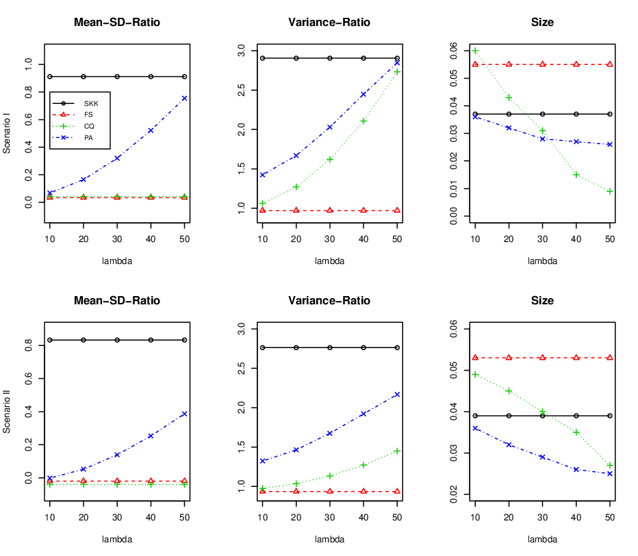
We examine the empirical sizes and the estimation efficiency of tests. Under the null hypothesis, the components of common vector ${\boldsymbol{\mu}}_{1}={\boldsymbol{\mu}}_{2}={\boldsymbol{\mu}}_{0}=(\mu_{1},\cdots,\mu_{p})$ are generated from $U(0,\lambda)$. The sample sizes are $n_{1}=n_{2}=15$. First, we consider the impact of dimension. We fix $\lambda=10$ and consider six dimensions $p=25,50,100,200,400,800$. We summarize simulation results by using the mean-standard deviation-ratio (MDR) $E(T)/\sqrt{\mathrm{var}(T)}$ and the variance ratio (VR) $\widehat{\mathrm{var}(T)}/\mathrm{var}(T)$. Since the explicit form of $E(T)$ and $\mathrm{var}(T)$ is difficult to calculate, we estimate them by simulation. Figure 1 reports the MDR, VR and empirical sizes of these four tests with different dimensions. We observe that MDR and VR of SKK test are larger than zero and one when the dimension becomes larger. It is not strange because SKK must require the dimension is a smaller order of $n^{2}$. Second, we consider the impact of common shifts. We fix the dimension $p=800$ and consider five common shifts $\lambda=10,20,30,40,50$. Figure 2 reports the MDR, VR and empirical sizes of these four tests with different common shifts. The MDR and VR of PA test become larger when the common shifts is larger. It further demonstrate that PA test is not shift-invariant. In contrast, the MDR and VR of our test is approximately zero and one, respectively. And then, we can control the empirical size very well. However, the empirical sizes of the other three tests deviate from the nominal level in most cases.

Figure 1: The MDR, VR and empirical sizes of tests with different dimensions.

Figure 2: The MDR, VR and empirical sizes of tests with different $\lambda$.

Next, we compare the power of all these tests. Here, we only report the case $n_{1}=n_{2}=15,p=800$. For the alternative hypothesis, ${\boldsymbol{\mu}}_{1}={\boldsymbol{\mu}}_{0}+{\boldsymbol{\mu}}$ and ${\boldsymbol{\mu}}_{2}={\boldsymbol{\mu}}_{0}$ where ${\boldsymbol{\mu}}_{0}$ are generated as above. We choose $\boldsymbol{\mu}$ in two scenarios: (Case A) one allocates all of the components of equal magnitude to be nonzero; (Case B) the other allocates randomly half of components of equal magnitude to be nonzero. To make the power comparable among the configurations of $H_{1}$, we set $\eta:=||\boldsymbol{\mu}_{1}-\boldsymbol{\mu}_{2}||^{2}/\sqrt{\mathrm{tr}({\boldsymbol{\Sigma}}_{1}^{2})+\mathrm{tr}({\boldsymbol{\Sigma}}_{2}^{2})}=0.15,0.2,0.25,0.3,0.35$ throughout the simulation. Figure 3 reports the empirical power of these four tests. Under Scenario II, CQ is less powerful than the other three tests because it is not scalar-invariant. Furthermore, our test performs better than SKK and PA tests in all cases. All these results together suggest that the newly proposed FS test is scale and shift invariant and quite efficient and robust in testing the equality of locations, and particularly useful when the variances of components are not equal and the dimension is ultra-high.

Figure 3: The power of tests with different $\eta$ when $n_{1}=n_{2}=15,p=800$.

Appendix: Proof of Theorem 1

Firstly, after some tedious calculations, we decompose $T_{n}$ into two parts, that is,

$$T_{n}= \frac{1}{n_{1}(n_{1}-1)}\frac{1}{n_{2}(n_{2}-1)}\sum_{k=1}^{p}\underset{i\not=j}{\sum^{n_{1}}\sum^{n_{1}}}\underset{s\not=t}{\sum^{n_{2}}\sum^{n_{2}}}\frac{(X_{1ik}-X_{2sk})(X_{1jk}-X_{2tk})}{{\sigma}^{2}_{1k}+\gamma{\sigma}^{2}_{2k}}$$

$$+\frac{1}{n_{1}(n_{1}-1)}\frac{1}{n_{2}(n_{2}-1)}\sum_{k=1}^{p}\underset{i\not=j}{\sum^{n_{1}}\sum^{n_{1}}}\underset{s\not=t}{\sum^{n_{2}}\sum^{n_{2}}}(X_{1ik}-X_{2sk})(X_{1jk}-X_{2tk})$$

$$~~~~~~~~~~~~~~~~~~~~~~~~~~\times\left(\frac{1}{\hat{\sigma}^{2}_{1k(i,j)}+\gamma\hat{\sigma}^{2}_{2k(s,t)}}-\frac{1}{{\sigma}^{2}_{1k}+\gamma{\sigma}^{2}_{2k}}\right)$$

$$\doteq T_{n1}+T_{n2}$$

Then, it is straightforward to see that

$$E(T_{n1}) =\sum_{k=1}^{p}\frac{(\mu_{1k}-\mu_{2k})^{2}}{\sigma_{1k}^{2}+\gamma\sigma_{2k}^{2}}=||{\bf\Lambda}(\boldsymbol{\mu}_{1}-\boldsymbol{\mu}_{2})||^{2},$$

$$\mathrm{var}(T_{n1}) =\frac{2}{n_{1}(n_{1}-1)}\mathrm{tr}(({\bf\Lambda}{\boldsymbol{\Sigma}}_{1}{\bf\Lambda})^{2})+\frac{2}{n_{2}(n_{2}-1)}\mathrm{tr}(({\bf\Lambda}{\boldsymbol{\Sigma}}_{2}{\bf\Lambda})^{2})+\frac{4}{n_{1}n_{2}}\mathrm{tr}({\bf\Lambda}{\boldsymbol{\Sigma}}_{1}{\bf\Lambda}^{2}{\boldsymbol{\Sigma}}_{2}{\bf\Lambda})$$

$$+\frac{4}{n_{1}}(\boldsymbol{\mu}_{1}-\boldsymbol{\mu}_{2})^{T}{\bf\Lambda}^{2}{\boldsymbol{\Sigma}}_{1}{\bf\Lambda}^{2}(\boldsymbol{\mu}_{1}-\boldsymbol{\mu}_{2})+\frac{4}{n_{2}}(\boldsymbol{\mu}_{1}-\boldsymbol{\mu}_{2})^{T}{\bf\Lambda}^{2}{\boldsymbol{\Sigma}}_{2}{\bf\Lambda}^{2}(\boldsymbol{\mu}_{1}-\boldsymbol{\mu}_{2}).$$

Lemma 1

Under the same conditions as Theorem 1, as $p$ and $n\to\infty$,

$$\frac{T_{n1}-E(T_{n1})}{\sqrt{\mathrm{var}(T_{n1})}}\overset{\mathcal{L}}{\longrightarrow}N(0,1).$$

This lemma is a direct corollary of Theorem 1 in Chen and Qin (2010).

Next, we only need to show that $T_{n2}=o_{p}(\sqrt{\mathrm{var}(T_{n1})})$. Define $Y_{ijk}=X_{ijk}-\mu_{ik}$, $i=1,2,j=1,\cdots,n_{i},k=1,\cdots,p$.

$$T_{n2}= \frac{1}{n_{1}(n_{1}-1)}\frac{1}{n_{2}(n_{2}-1)}\sum_{k=1}^{p}\underset{i\not=j}{\sum^{n_{1}}\sum^{n_{1}}}\underset{s\not=t}{\sum^{n_{2}}\sum^{n_{2}}}(Y_{1ik}-Y_{2sk})(Y_{1jk}-Y_{2tk})$$

$$~~~~~~~~~~~~~~~~~~~~~~~~~~\times\left(\frac{1}{\hat{\sigma}^{2}_{1k(i,j)}+\gamma\hat{\sigma}^{2}_{2k(s,t)}}-\frac{1}{{\sigma}^{2}_{1k}+\gamma{\sigma}^{2}_{2k}}\right)$$

$$+\frac{2}{n_{1}n_{2}}\sum_{k=1}^{p}\sum_{i=1}^{n_{1}}\sum_{s=1}^{n_{2}}(Y_{1ik}-Y_{2sk})(\mu_{1k}-\mu_{2k})$$

$$~~~~~~~~~~~~~~~~~~~~~~~~~~\times\left(\frac{1}{\hat{\sigma}^{2}_{1k(i,j)}+\gamma\hat{\sigma}^{2}_{2k(s,t)}}-\frac{1}{{\sigma}^{2}_{1k}+\gamma{\sigma}^{2}_{2k}}\right)$$

$$+\sum_{k=1}^{p}(\mu_{1k}-\mu_{2k})^{2}\left(\frac{1}{\hat{\sigma}^{2}_{1k(i,j)}+\gamma\hat{\sigma}^{2}_{2k(s,t)}}-\frac{1}{{\sigma}^{2}_{1k}+\gamma{\sigma}^{2}_{2k}}\right)$$

$$\doteq R_{1}+R_{2}+R_{3}$$

Define ${\bf\Lambda}_{(i,j,s,t)}=\mathrm{diag}\{(\hat{\sigma}_{11(i,j)}^{2}+\gamma\hat{\sigma}_{21(s,t)}^{2})^{-1/2},\cdots,(\hat{\sigma}_{1p(i,j)}^{2}+\gamma\hat{\sigma}_{2p(s,t)}^{2})^{-1/2}\}$.

$$R_{1}= \frac{1}{n_{2}(n_{2}-1)}\sum_{t\not=s}^{n_{2}}\sum_{s=1}^{n_{2}}\left(\frac{1}{n_{1}(n_{1}-1)}\sum^{n_{1}}_{j\not=i}\sum^{n_{1}}_{i=1}{\bf Y}_{1i}^{T}(\hat{{\bf\Lambda}}_{(i,j,s,t)}^{2}-{\bf\Lambda}^{2}){\bf Y}_{1j}\right)$$

$$+\frac{1}{n_{1}(n_{1}-1)}\sum^{n_{1}}_{j\not=i}\sum^{n_{1}}_{i=1}\left(\frac{1}{n_{2}(n_{2}-1)}\sum_{t\not=s}^{n_{2}}\sum_{s=1}^{n_{2}}{\bf Y}_{2s}^{T}(\hat{{\bf\Lambda}}_{(i,j,s,t)}^{2}-{\bf\Lambda}^{2}){\bf Y}_{2t}\right)$$

$$-\frac{2}{(n_{1}-1)(n_{2}-1)}\sum_{j\not=i}^{n_{1}}\sum_{s\not=t}^{n_{2}}\left(\frac{1}{n_{1}n_{2}}\sum_{i=1}^{n_{1}}\sum_{s=1}^{n_{2}}{\bf Y}_{1i}^{T}(\hat{{\bf\Lambda}}_{(i,j,s,t)}^{2}-{\bf\Lambda}^{2}){\bf Y}_{2t}\right)$$

By the Theorem 1 in Park and Ayyala (2013), we have

$$E\left(\frac{1}{n_{1}(n_{1}-1)}\sum^{n_{1}}_{j\not=i}\sum^{n_{1}}_{i=1}{\bf Y}_{1i}^{T}(\hat{{\bf\Lambda}}_{(i,j,s,t)}^{2}-{\bf\Lambda}^{2}){\bf Y}_{1j}\right)^{2}=O(n^{-3}\mathrm{tr}(({\bf\Lambda}{\boldsymbol{\Sigma}}_{1}{\bf\Lambda})^{2}))=o(\mathrm{var}(T_{n1}))$$

$$E\left(\frac{1}{n_{2}(n_{2}-1)}\sum_{t\not=s}^{n_{2}}\sum_{s=1}^{n_{2}}{\bf Y}_{2s}^{T}(\hat{{\bf\Lambda}}_{(i,j,s,t)}^{2}-{\bf\Lambda}^{2}){\bf Y}_{2t}\right)^{2}=O(n^{-3}\mathrm{tr}(({\bf\Lambda}{\boldsymbol{\Sigma}}_{2}{\bf\Lambda})^{2}))=o(\mathrm{var}(T_{n1}))$$

$$E\left(\frac{1}{n_{1}n_{2}}\sum_{i=1}^{n_{1}}\sum_{s=1}^{n_{2}}{\bf Y}_{1i}^{T}(\hat{{\bf\Lambda}}_{(i,j,s,t)}^{2}-{\bf\Lambda}^{2}){\bf Y}_{2t}\right)^{2}=O(n^{-3}\mathrm{tr}({\bf\Lambda}{\boldsymbol{\Sigma}}_{1}{\bf\Lambda}^{2}{\boldsymbol{\Sigma}}_{2}{\bf\Lambda}))=o(\mathrm{var}(T_{n1}))$$

Thus, $R_{1}=o_{p}(\sqrt{\mathrm{var}(T_{n1})})$. Similarly,

$$R_{2}= \frac{2}{n_{2}(n_{2}-1)(n_{1}-1)}\sum_{t\not=s}^{n_{2}}\sum_{s=1}^{n_{2}}\sum_{j\not=i}^{n_{1}}\left(\frac{1}{n_{1}}\sum_{i=1}^{n_{1}}{\bf Y}_{1i}^{T}(\hat{{\bf\Lambda}}_{(i,j,s,t)}^{2}-{\bf\Lambda}^{2})({\boldsymbol{\mu}}_{1}-{\boldsymbol{\mu}}_{2})\right)$$

$$-\frac{2}{n_{1}(n_{1}-1)(n_{2}-1)}\sum_{j\not=i}^{n_{1}}\sum_{i=1}^{n_{1}}\sum_{t\not=s}^{n_{2}}\left(\frac{1}{n_{2}}\sum_{s=1}^{n_{1}}{\bf Y}_{2s}^{T}(\hat{{\bf\Lambda}}_{(i,j,s,t)}^{2}-{\bf\Lambda}^{2})({\boldsymbol{\mu}}_{1}-{\boldsymbol{\mu}}_{2})\right)$$

By the proof of Theorem 2 in Park and Ayyala (2013), we have

$$E\left(\frac{1}{n_{1}}\sum_{i=1}^{n_{1}}{\bf Y}_{1i}^{T}(\hat{{\bf\Lambda}}_{(i,j,s,t)}^{2}-{\bf\Lambda}^{2})({\boldsymbol{\mu}}_{1}-{\boldsymbol{\mu}}_{2})\right)^{2}=O(n^{-2}({\boldsymbol{\mu}}_{1}-{\boldsymbol{\mu}}_{2})^{T}{\bf\Lambda}^{2}{\boldsymbol{\Sigma}}_{1}{\bf\Lambda}^{2}({\boldsymbol{\mu}}_{1}-{\boldsymbol{\mu}}_{2}))$$

$$E\left(\frac{1}{n_{2}}\sum_{s=1}^{n_{1}}{\bf Y}_{2s}^{T}(\hat{{\bf\Lambda}}_{(i,j,s,t)}^{2}-{\bf\Lambda}^{2})({\boldsymbol{\mu}}_{1}-{\boldsymbol{\mu}}_{2})\right)^{2}=O(n^{-2}({\boldsymbol{\mu}}_{1}-{\boldsymbol{\mu}}_{2})^{T}{\bf\Lambda}^{2}{\boldsymbol{\Sigma}}_{2}{\bf\Lambda}^{2}({\boldsymbol{\mu}}_{1}-{\boldsymbol{\mu}}_{2}))$$

By the Condition (C3), we also have $R_{2}=o_{p}(\sqrt{\mathrm{var}(T_{n1})})$. And $E(R_{3}^{2})=O(n^{-1}(({\boldsymbol{\mu}}_{1}-{\boldsymbol{\mu}}_{2})^{T}{\bf\Lambda}({\boldsymbol{\mu}}_{1}-{\boldsymbol{\mu}}_{2}))^{2})=o(\mathrm{var}(T_{n1}))$. Thus, we proof that $T_{n2}=o_{p}(\sqrt{\mathrm{var}(T_{n1})})$.

References

Anderson, T. W. 2003. An Introduction to Multivariate Statistical Analysis, Hoboken, NJ: Wiley.

Bai Z. and Saranadasa, H. 1996. Effect of high dimension: by an example of a two sample problem, Statistica Sinica, 6, 311–329.

Biswas, M. and Ghosh. A. K. 2014. A nonparametric two-sample test applicable to high dimensional data, Journal of Multivariate Analysis, 123, 160–171.

Cai, T., Liu, W. D. and Xia, Y. 2013. Two-sample test of high dimensional means under dependency, Journal of the Royal Statistical Society: Series B, 76, 349–372.

Chen, L. S., Paul, D., Prentice, R. L. and Wang, P. 2011. A regularized Hotelling’s $T^{2}$ test for pathway analysis in proteomic studies, Journal of the American Statistical Association, 106, 1345–1360.

Chen, S. X. and Qin, Y-L. 2010. A two-sample test for high-dimensional data with applications to gene-set testing, The Annals of Statistics, 38, 808–835.

Dempster, A. P. 1958. A high dimensional two sample significance test, The Annals of Mathematical Statistics, 29, 995–1010.

Feng, L., Zou, C., Wang, Z. and Zhu, L. 2014. Two sample Behrens-Fisher problem for high-dimensional data. Statistica Sinica, To appear.

Gregory, K. B., Carroll, R. J., Baladandayuthapani, V. and Lahiri, S. N. 2014. A two-sample test for equality of means in high dimension, Journal of the American Statistical Association, To appear.

Park, J. and Ayyala, D. N. 2013. A test for the mean vector in large dimension and small samples, Journal of Statistical Planning and Inference, 143, 929-943.

Srivastava, M. S. and Du, M. 2008. A test for the mean vector with fewer observations than the dimension, Journal of Multivariate Analysis, 99, 386–402.

Srivastava, M. S., Katayama, S. and Kano, Y. 2013. A two sample test in high dimensional data, Journal of Multivariate Analysis, 114, 349–358.

Zhang, J. T. and Xu, J. F. 2009. On the $k$-sample Behrens-Fisher problem for high-dimensional data, Science in China Series A: Mathematics, 52, 1285–1304.