Modeling high-frequency order flow imbalance by functional limit theorems for two-sided risk processesThanks: Research supported by Russian Scientific Foundation, project 14-11-00364.

Abstract: A micro-scale model is proposed for the evolution of the limit order book. Within this model, the flows of orders (claims) are described by doubly stochastic Poisson processes taking account of the stochastic character of intensities of bid and ask orders that determine the price discovery mechanism in financial markets. The process of order flow imbalance (OFI) is studied. This process is a sensitive indicator of the current state of the limit order book since time intervals between events in a limit order book are usually so short that price changes are relatively infrequent events. Therefore price changes provide a very coarse and limited description of market dynamics at time micro-scales. The OFI process tracks best bid and ask queues and change much faster than prices. It incorporates information about build-ups and depletions of order queues so that it can be used to interpolate market dynamics between price changes and to track the toxicity of order flows. The two-sided risk processes are suggested as mathematical models of the OFI process. The multiplicative model is proposed for the stochastic intensities making it possible to analyze the characteristics of order flows as well as the instantaneous proportion of the forces of buyers and sellers, that is, the intensity imbalance (II) process, without modeling the external information background. The proposed model gives the opportunity to link the micro-scale (high-frequency) dynamics of the limit order book with the macro-scale models of stock price processes of the form of subordinated Wiener processes by means of functional limit theorems of probability theory and hence, to give a deeper insight in the nature of popular subordinated Wiener processes such as generalized hyperbolic Lévy processes as models of the evolution of characteristics of financial markets. In the proposed models, the subordinator is determined by the evolution of the stochastic intensity of the external information flow.

Key words: financial markets; limit order book; price discovery; number of orders imbalance; order flow imbalance; doubly stochastic Poisson processes; Cox processes; variance-mean mixture; normal mixture; two-sided risk process; Lévy process; generalized hyperbolic Lévy process; generalized inverse Gaussian distribution

1 Introduction

High-frequency trading became a significant portion of the trading volume on equity, futures and options exchanges. The high-frequency behavior of the so-called limit order book, the list of trading orders, is now a popular object of stochastic modeling, see, e.g., [53], [28], [32], [2], [55]. R. Cont et al. [18] proposed a continuous-time Markov model for the limit order book dynamics. In the paper [18] the limit order book is considered as a special queuing system where incoming orders and cancelations of existing orders of unit sizes arrive according to independent Poisson processes. Such kind of queuing system can be described in terms of birth-death processes, where the states represent the number of shares at a given order price, and transitions take place by birth (the entry of a new limit order), or death (removal from the limit order book by cancelation or matching with a new market order). Birth-death processes are well-studied statistical models which can be regarded as special examples of more general two-sided risk processes, the stochastic models known in insurance mathematics as risk processes with stochastic premiums.

A queueing-system-type mathematical model for the limit order book [18] is supplied with rather strict formal a priori conditions. For instance, one of such conditions is that the intensities of order flows are assumed constant. On the one hand, these assumptions provide the possibility to calculate at least some characteristics of the limit order book dynamics. However, on the other hand, these assumptions turn out to be too restrictive and unrealistic from the practical point of view. Therefore, it is extremely desirable to have a convenient integral characteristic of the current state of the limit order book which can be calculated and studied without the queueing systems framework.

Such a characteristic, the order flow imbalance $($OFI$)$ process, was introduced in 2011 in the paper [21], the final version of which [22] was published in 2014. The same process was independently introduced and studied in [44, 49, 50, 16] under the name of generalized price process. The OFI process appears to be considerably more sensitive to the market information than the price process itself. This is due to that time intervals that are involved in modern high-frequency trading applications are usually so short that price changes are relatively infrequent events. Therefore price changes provide a very coarse and limited description of market dynamics. However, OFI takes account of not only best ask and bid changes, but also the arrivals/cancelations of orders deep inside the limit order book, which is of interest and importance because each such event influences the current balance between buyers and sellers and fluctuates on a much faster timescale than prices. It incorporates information about build- ups and depletions of order queues and it can be used to interpolate market dynamics between price changes.

In the framework of the approach developed in the present paper the principal idea is that the moments at which the state of the limit order book changes form a chaotic point stochastic process on the time axis. Moreover, this point process turns out to be non-stationary (time-non-homogeneous) because the changes of the state of the limit order book are to a great extent subject to the influence of non-stationary information flows. As is known, most reasonable probabilistic models of non-stationary (time-non-homogeneous) chaotic point processes are doubly stochastic Poisson processes also called Cox processes (see, e. g., [33, 10]). These processes are defined as Poisson processes with stochastic intensities. Pure Poisson processes can be regarded as best models of stationary (time-homogeneous) chaotic flows of events [10]. Recall that the attractiveness of a Poisson process as a model of homogeneous discrete stochastic chaos is due to at least two reasons. First, Poisson processes are point processes characterized by that time intervals between successive points are independent random variables with one and the same exponential distribution and, as is well known, the exponential distribution possesses the maximum differential entropy among all absolutely continuous distributions concentrated on the nonnegative half-line with finite expectations, whereas the entropy is a natural and convenient measure of uncertainty. Second, the points forming the Poisson process are uniformly distributed along the time axis in the sense that for any finite time interval $[t_{1},t_{2}]$, $t_{1}<t_{2}$, the conditional joint distribution of the points of the Poisson process which fall into the interval $[t_{1},t_{2}]$ under the condition that the number of such points is fixed and equals, say, $n$, coincides with the joint distribution of the order statistics constructed from an independent sample of size $n$ from the uniform distribution on $[t_{1},t_{2}]$ whereas the uniform distribution possesses the maximum differential entropy among all absolutely continuous distributions concentrated on finite intervals and very well corresponds to the conventional impression of an absolutely unpredictable random variable (see, e. g., [31, 10]).

Financial markets are examples of complex open systems whose behavior is subject to randomness of two types: internal (endogenous) and external (exogenous). The internal source produces the uncertainty due to the difference of the strategies of a very large number of traders. The <<physical>> analog of such a randomness is the chaotic thermal motion of particles in closed systems. The external source of randomness is a poorly predictable flow of political or economical news influencing the interests and strategies of traders. These two sources of randomness will be taken into account when we construct the models of order flow imbalance process and number of orders imbalance process as two-sided risk processes driven by a Cox process, that is, by a Poisson process with stochastic intensity.

As is known, the empirical (statistical) distributions of increments of (the logarithms of) financial indices and, in particular, of stock prices on comparatively short time intervals have significantly heavy-tailed distributions with vertices noticeably sharper than those of normal distributions, that is, they are leptokurtic. At the same time, as is observed in some studies, financial time series possess the fractal property, that is, they are to some extent self-similar at different time scales, see, e. g., [52].

Stable Lévy processes were among the first models applied in practice successfully explaining the observed leptokurticity of finite-dimensional distributions of the processes in financial markets as well as their self-similarity. According to the approach based on classical limit theorems of probability theory, non-normal stable Lévy processes can appear as limits in functional limit theorems for random walks only if the variances of elementary jumps are infinite. In [20] some diffusive-type functional limit theorems were proved for the dynamics of limit order books in liquid markets and it was especially indicated that within the approach used in that paper it is possible to obtain stable limit processes only if the order sizes posses infinite variances. In turn, the latter is possible only if the probabilities of arbitrarily large jumps are positive. Unfortunately, the latter condition looks very doubtful from the practical viewpoint. Therefore, within the framework of the classical approach used in [52] and [20], the theoretical explanation of stable Lévy processes as adequate models for the evolution of stock prices or financial indexes is at least questionable.

In financial mathematics the evolution of (the logarithms of) stock prices and financial indexes on small time horizons is often modeled by random walks. The simplest example of such an approach is the Cox–Ross–Rubinstein model (see, e. g., [60]). At the same time most successful (adequate) models of the dynamics of (the logarithms of) financial indexes on large time horizons are subordinated Wiener processes (processes of Brownian motion with random time) such as generalized hyperbolic processes, in particular, variance gamma (VG) processes and normal$\backslash\!\backslash$inverse Gaussian (NIG) processes, see [60]. Subordinated Wiener processes have finite-dimensional distributions possessing the properties mentioned above: these distributions are heavy-tailed and leptokurtic.

In [17, 38] and [31] the heavy-tailedness of the empirical distributions of stock prices was explained with the use of limit theorems for sums of a random number of independent random variables as a particular case of randomly stopped random walks.

When random walks are considered, the scheme of random summation is a natural analog of the scheme of subordination of more general random processes. In [31, 41, 42] it was proposed to model the evolution of non-homogeneous chaotic stochastic processes, in particular, of the dynamics of stock prices and financial indexes, by random walks generated by compound doubly stochastic Poisson processes (compound Cox pocesses). A doubly stochastic Poisson process (also called a Cox process) is a stochastic point process of the form $N_{1}(\Lambda(t))$, where $N_{1}(t)$, $t\geq 0$, is a homogeneous Poisson process with unit intensity and the stochastic process $\Lambda(t)$, $t\geq 0$, is independent of $N_{1}(t)$ and possesses the following properties: $\Lambda(0)=0$, ${\sf P}(\Lambda(t)<\infty)=1$ for any $t>0$, the sample paths of $\Lambda(t)$ do not decrease and are right-continuous. A compound Cox process is a random sum of independent identically distributed random variables in which the number of summands follows a Cox process. Similar continuous-time random walks were considered in [34, 62, 35].

In accordance with the approach used in [31, 41, 42] the limit distributions for compound Cox process with elementary jumps possessing finite variances must have the form of scale-location mixtures of normal laws which are always heavy-tailed and leptokurtic, if the mixing distribution is non-degenerate. Moreover, in [39, 40] it was shown that non-normal stable laws can appear as limit distributions for sums of independent identically distributed random variables with finite variances, if the number of summands in the sum is random and its distribution converges to a stable law concentrated on the nonnegative half-line. In terms of compound Cox processes the latter condition means that finite-dimensional distributions of the leading process $\Lambda(t)$ are asymptotically stable. In turn, this means that the intensity of the flow of informative events is essentially irregular which results in the well-known clustering effect.

In [48] some functional limit theorems were proved establishing convergence of random walks generated by compound Cox processes with jumps possessing finite variances to Lévy processes with symmetric distributions including symmetric strictly stable Lévy processes. Here we extend these results to a non-symmetric case and apply them to modeling the evolution of the OFI process, an integral characteristic of the behavior of the limit order book.

Functional limit theorems are a quite natural link between random walks and subordinated Wiener processes. The operation of subordination gives a good explanation of the presence of heavy tails in the empirical distributions of the increments of (the logarithms of) stock prices and financial indexes. The functional limit theorems for compound Cox processes proved in [48] serve as a bridge between formal micro-scale models having the form of continuous-time random walks generated by compound Cox processes and popular macro-scale models of the form of subordinated Wiener processes including generalized hyperbolic processes, variance gamma processes, etc. The practical importance of these models is justified by the stochastic character of the intensities of chaotic flows of informative events in large financial information systems and, in particular, in high-frequency trading systems. The use of high-frequency statistical data available due to electronic trading systems makes it possible to verify the models mentioned above and to link them with the price discovery process resulting from the limit order book evolution.

This paper presents a further development of the models and techniques proposed in our previous papers [44], [49], [16]. In this paper we propose a convenient and rather realistic model for the OFI process using the notion of two-sided risk processes. For this purpose we use the techniques developed in [48].

The paper is organized as follows. We construct our model step by step. In Section 2 we give necessary definitions and under the condition that the intensities of order flows are constant introduce the two-sided risk process adopting the notion of a risk process with stochastic premiums from insurance mathematics and prove that it is a special compound Poisson process. In Section 3 we introduce the conditional non-homogeneous OFI process, introduce the multiplicative representation for the intensities of order flows in the limit order book and, finally, introduce the assumption that the intensity of the external information flow is stochastic and obtain the general (unconditional) OFI process as a special compound doubly stochastic Poisson process. The remaining part of the paper is devoted to functional limit theorems for the so-defined OFI process. Section 4 contains some preliminary material on the Skorokhod space and Lévy processes. In section 5 we prove general functional limit theorem establishing the conditions for convergence of OFI processes to Lévy processes in the Skorokhod space in terms of the behavior of the intensities of order flow. For this purpose we slightly extend the classical results presented, say, in [36]. In Section 6 we consider the conditions for the convergence of OFI processes with elementary jumps (that is, order sizes) possessing finite variances to the Lévy processes with variance-mean mixed normal one-dimensional distributions, that is, to subordinated Wiener processes, in particular, to generalized hyperbolic Lévy processes. In Section 7 we discuss empirical results and the final adjustment of the model.

2 Basic model of order book dynamics and conditional homogeneous order flow imbalance process

Market participants trading an asset in an order-driven market can undertake three different kinds of actions. They may

• place a limit order to buy or sell a specified number of shares of the asset at a particular price specified at the time of the order,

• place a market order to buy or sell a specified number of shares of the asset at the best currently available price, which is executed immediately, or

• cancel a previously placed limit order that has not yet been executed.

The outstanding limit orders are summarized in a limit order book, which lists the total number of shares of buy and sell limit orders at each price. This limit order book is constantly changing as new orders arrive, and we are interested in modeling statistical properties of the limit order book state. The limit buy orders are called bids, and the limit sell orders are called asks. The size of the order is the number of shares specified by the order. The lowest price for which there is an outstanding limit sell order is called the best ask and the highest price for which there is an outstanding limit buy order is called the best bid. The gap between the best ask and the best bid is called the bid-ask spread. The average of the best ask and best bid is called the mid-price.

Of course, a limit order can turn turn out to be a market order, if the price specified in it allows immediate matching with one of the limit orders on the opposite side of the limit order book.

We consider the dynamics of the limit order book on the discrete price lattice $\Pi=\{1,2,...,M\}$ as a continuous-time process

$$\mathbf{x}(t)\equiv(\mathbf{V^{a}}(t);\mathbf{V^{b}}(t))\equiv(V^{a}_{1}(t),V^{a}_{2}(t),...,V^{a}_{M}(t);V^{b}_{1}(t),V^{b}_{2}(t),...,V^{b}_{M}(t)),\ \ \ t\geqslant 0,$$

where $V^{a}_{p}(t)$ ($V^{b}_{p}(t))$ is the number of sell (buy) limit orders with price $p\in\Pi$. Since buy and sell orders with one and the same specified price cannot exist at a time (otherwise they are immediately matched), we necessarily have $V^{a}_{p}(t)\vee V^{b}_{p}(t)=0$ for all $p\in\Pi$ and $t$.

The best ask $a(t)$ is defined as $a(t)=\inf\{p:V^{a}_{p}(t)>0\}\wedge(M+1)$, the best bid $b(t)$ is $b(t)=\sup\{p:V^{b}_{p}(t)>0\}\vee 0$. Correspondingly, the mid-price is defined as $P(t)=\frac{1}{2}[a(t)+b(t)]$. Thus, the price process $P(t)$ is a result of the evolution of the limit order book generated by the flow of orders of three types.

First let us assume that the information flow coming from the outer medium is fixed. Then, under fixed information, we can assume that the inner randomness has a stable chaotic character. As it has already been said in Sect. 1, Poisson processes are natural mathematical models of continuous-time chaotic point processes characterized by that the intervals between informative events (arrivals of orders) are independent identically distributed random variables with exponential distribution, see, e. g., [31, 42, 43]. Therefore, on the first stage of the construction of our model the order flows are assumed to be independent renewal processes with exponentially distributed interrenewal times (as it was done, e. g., in the papers [18], [20]):

• limit buy (sell) orders independently arrive at a price level situated at the distance $i$ from the best ask (bid) so that the time intervals between successive arrivals have exponential distribution with parameter $\lambda_{i}^{+}>0$ $(\lambda_{i}^{-}>0)$ (empirical studies [64] and [13] show that the power law $\lambda_{i}^{\pm}=ki^{-\alpha}$ is a good approximation);

• market buy (sell) orders arrive independently so that the time intervals between successive arrivals have exponential distribution with parameter $\mu^{+}$ $(\mu^{-})$;

• cancelations of a limit buy (sell) order at a price level situated at the distance $i$ from the best bid (ask) arrive with frequency $\theta_{i}^{+}$ $(\theta_{i}^{-})$.

Under the above assumptions, $\mathbf{x}(t)$ is a continuous-time Markov chain with state space $(\mathbb{Z}^{+})^{2M}$ and the transitions

$$V^{a}_{i}(t)\to V^{a}_{i}(t)+1 \text{ with intensity }\lambda^{-}_{i-b(t)} \text{ for }i>b(t),$$

$$V^{a}_{i}(t)\to V^{a}_{i}(t)-1 \text{ with intensity }\theta^{-}_{i-a(t)} \text{ for }i\geqslant a(t),$$

$$V^{a}_{i}(t)\to V^{a}_{i}(t)-1 \text{ with intensity }\mu^{+} \text{ for }i=a(t)>0.$$

$$V^{b}_{i}(t)\to V^{b}_{i}(t)+1 \text{ with intensity }\lambda^{+}_{a(t)-i} \text{ for }i<a(t),$$

$$V^{b}_{i}(t)\to V^{b}_{i}(t)-1 \text{ with intensity }\theta^{+}_{b(t)-i} \text{ for }i\leqslant b(t),$$

$$V^{b}_{i}(t)\to V^{b}_{i}(t)-1 \text{ with intensity }\mu^{-} \text{ for }i=b(t)<M+1.$$

Thus, we can define the following independent Poisson processes:

• $L^{\pm}_{i}(t):$ the flows of limit orders with intensities $\lambda_{i}^{\pm}$;

• $M^{\pm}(t):$ the flows of market orders with intensities $\mu^{+}\mathbb{I}(\mathbf{V^{a}}\neq 0)$ and $\mu^{-}\mathbb{I}(\mathbf{V^{b}}\neq 0)$;

• $C^{\pm}_{i}(t):$ the flows of cancelations of limit orders with intencities $\theta_{i}^{\pm}$,

and the Poisson process

$$N(t)=M^{+}(t)+M^{-}(t)+\sum\nolimits_{i=1}^{M}(L_{i}^{+}(t)+L_{i}^{-}(t))+\sum\nolimits_{i=1}^{M}(C_{i}^{+}(t)+C_{i}^{-}(t)),$$

which describes the flow of all arriving orders.

The processes $L^{\pm}_{i}(t)$, $M^{\pm}(t)$, $C^{\pm}_{i}(t)$ completely determine the price process $P(t)$ for which the corresponding stochastic differential equations can be written out [1]. However, its further analytical interpretation is very difficult or even impossible even under rather strong and unrealistic assumption that the intensities of the flows of orders of different types are constant.

It seems reasonable to consider some indicator of the current state of the limit order book taking account of not only best ask and bid changes, but also the arrivals/cancelations of orders deep inside the limit order book, which is of interest and importance because each such event influences the current balance of the forces of buyers and sellers.

Recall that for the time being the intensity of the external information flow is assumed to be fixed (constant). First fix a time interval $[0,T]$ which is rather small so that the intensities of the events described above can be assumed constant within this interval. Let, as above, $N(t)$, $t\in[0,T]$, be the Poisson process counting all the events in the limit order book and having the intensity

$$\lambda=\mu^{+}+\mu^{-}+\sum\nolimits_{i=1}^{M}(\lambda_{i}^{+}+\lambda_{i}^{-})+\sum\nolimits_{i=1}^{M}(\theta_{i}^{+}+\theta_{i}^{-}).$$

Split $N(t)$ into the sum of two independent Poisson processes $N^{+}(t)$ and $N^{-}(t)$ with the corresponding intensities

$$\lambda^{+}=\mu^{+}+\sum\nolimits_{i=1}^{M}\lambda_{i}^{+}+\sum\nolimits_{i=1}^{M}\theta_{i}^{-}$$

and

$$\lambda^{-}=\mu^{-}+\sum\nolimits_{i=1}^{M}\lambda_{i}^{-}+\sum\nolimits_{i=1}^{M}\theta_{i}^{+}.$$

Thus, $\lambda=\lambda^{+}+\lambda^{-}$ and the processes $N^{+}(t)$ and $N^{-}(t)$ characterize the cumulative force of buyers and sellers, correspondingly (note that a cancelation of sell orders increases the force of buyers and vice versa). The processes $N^{+}(t)$ and $N^{-}(t)$ are conditionally independent under fixed outer information flow during the time interval $[0,t]$.

Following [50], consider the following model of a conditional homogeneous OFI process. Let $X_{1}^{+},X_{2}^{+},...$ be identically distributed non-negative random variables corresponding to sequential buy order sizes and also let $X_{1}^{-},X_{2}^{-},...$ be identically distributed nonnegative random variables corresponding to sequential sell order sizes. Let $N_{1}^{-}(t)$ and $N_{1}^{+}(t)$ be two standard Poisson processes (that is, homogeneous Poisson processes with unit intensities). Assume that for each $t$, the random variables $X_{1}^{+},X_{2}^{+},...$, $X_{1}^{-},X_{2}^{-},...$, $N_{1}^{-}(t)$ and $N_{1}^{+}(t)$ are independent. Introduce the process

$$Q^{(CH)}(t)=\sum\nolimits_{j=1}^{N_{1}^{+}(\lambda^{+}t)}X_{j}^{+}-\sum\nolimits_{j=1}^{N_{1}^{-}(\lambda^{-}t)}X_{j}^{-}.$$

The process $Q^{(CH)}(t)$ will be called the conditional homogeneous OFI process. This process is an integral instantaneous characteristic of the state of the limit order book under the ideal condition that the intensity of the external information flow does not change.

Formally, the process $Q^{(CH)}(t)$ introduced above is nothing else but what is well known in insurance mathematics as the risk process with stochastic premiums, the positive term of which describes the flow of insurance premiums while the negative term describes the flow of insurance claims, see, e. g., [43]. However, as it was especially noted in [43], such models can hardly be assumed adequate in insurance practice because the two components of $Q^{(CH)}(t)$ are independent whereas in real insurance practice the counting process in the negative component of $Q^{(CH)}(t)$ is a rarefaction of that in the positive component and, hence, the components cannot be assumed stochastically independent in insurance practice. Nevertheless, as it was also noted in [43], model (1) can be successfully applied to the description of the processes of speculative financial activity. In financial applications, processes of type (1) describe the balance of forces of buyers and sellers and the resulting risks. Hence, in what follows we will use a terminology more appropriate for the financial applications and call the processes of form (1) two-sided risk processes.

Lemma 1. Under the above assumptions, $Q^{(CH)}(t)$ is a compound Poisson process. Namely, if $N_{1}(t)$ is the standard Poisson process, then for each $t\geqslant 0$

$$Q^{(CH)}(t)\stackrel{{\scriptstyle d}}{{=}}\sum\nolimits_{j=1}^{N_{1}((\lambda^{+}+\lambda^{-})\,t)}X_{j},$$

where $X_{1},X_{2},...$ are identically distributed random variables with the common characteristic function

$$\mathfrak{f}(s)\equiv{\sf E}e^{isX_{1}}=\frac{\lambda^{+}\mathfrak{f}^{+}(s)}{\lambda^{+}+\lambda^{-}}+\frac{\lambda^{-}\mathfrak{f}^{-}(-s)}{\lambda^{+}+\lambda^{-}},\ \ \ s\in\mathbb{R},$$

where $\mathfrak{f}^{+}(s)$ and $\mathfrak{f}^{-}(s)$ are the characteristic functions of the random variables $X_{1}^{+}$ and $X_{1}^{-}$, respectively. Moreover, for each $t\geqslant 0$ the random variables $N_{1}\big((\lambda^{+}+\lambda^{-})\,t\big)$, $X_{1},X_{2},...$ are independent.

Proof. Since $Q^{(CH)}(t)$ is a difference of two independent homogeneous processes with independent increments, it also possesses these properties. So, it remains to consider its characteristic function. We obviously have

$$\mathfrak{f}_{Q^{(CH)}(t)}(s)\equiv{\sf E}e^{isQ^{(CH)}(t)}=\exp\big\{\lambda^{+}t\big(\mathfrak{f}^{+}(s)-1\big)\big\}\exp\big\{\lambda^{-}t\big(\mathfrak{f}^{-}(-s)-1\big)\big\}=$$

$$\exp\bigg\{(\lambda^{+}+\lambda^{-})t\bigg[\frac{\lambda^{+}\mathfrak{f}^{+}(s)}{\lambda^{+}+\lambda^{-}}+\frac{\lambda^{-}\mathfrak{f}^{-}(-s)}{\lambda^{+}+\lambda^{-}}\bigg]-1\bigg\},\ \ \ s\in\mathbb{R}.$$

The latter characteristic function corresponds to the compound Poisson distribution specified in the formulation of the lemma.

Remark 1. It is easy to see that the random variable $X_{1}$ is a randomization:

$$X_{1}=\begin{cases}X_{1}^{+}&\text{with probability }{\displaystyle\frac{\lambda^{+}}{\lambda^{+}+\lambda^{-}}},\\ -X_{1}^{-}&\text{with probability }{\displaystyle\frac{\lambda^{-}}{\lambda^{+}+\lambda^{-}}}\end{cases}$$

so that

$${\sf E}X_{1}=\frac{\lambda^{+}{\sf E}X_{1}^{+}}{\lambda^{+}+\lambda^{-}}-\frac{\lambda^{-}{\sf E}X_{1}^{-}}{\lambda^{+}+\lambda^{-}},$$

$${\sf D}X_{1}=\bigg(\frac{\lambda^{+}}{\lambda^{+}+\lambda^{-}}\bigg)^{2}{\sf D}X_{1}^{+}+\bigg(\frac{\lambda^{-}}{\lambda^{+}+\lambda^{-}}\bigg)^{2}{\sf D}X_{1}^{-}-\frac{\lambda^{+}\lambda^{-}}{(\lambda^{+}+\lambda^{-})^{2}}{\sf E}\big(X_{1}^{+}-X_{1}^{-}\big)^{2}.$$

Some empirical studies (see, e. g., [15, 61]) show that new limit order sizes are in fact randomly distributed according to the exponential law resulting in that within model (2), in general, the distribution of independent random variables $X_{j}$ is the asymmetric Laplace law (a mixture of the exponential distribution and the distribution symmetric to exponential concentrated on the negative half-line).

3 General order flow imbalance process

In this section the ideal conditional model described above will be adapted with the account of non-constant character of the intensity of external information flow resulting in that the parameters $\lambda^{+}$ and $\lambda^{-}$ describing the corresponding reaction of buyers and sellers vary in time.

In reality, the intensities of the order flows are non-homogeneous since the external information flow determining the intensities of the events in the order book is non-homogeneous itself. In this case the intensities of the flows of orders of different types, first, may not be independent and, second, depend in a certain way on some process which determines the external news background. To formalize these ideas, assume that the intensities of the processes introduced in Sect. 2 vary in time:

$$\mu^{+}=\mu^{+}(t),\ \ \lambda^{+}_{i}=\lambda^{+}_{i}(t),\ \ \ \theta^{+}_{i}=\theta^{+}_{i}(t),$$

$$\mu^{-}=\mu^{-}(t),\ \ \lambda^{-}_{i}=\lambda^{-}_{i}(t),\ \ \ \theta^{-}_{i}=\theta^{-}_{i}(t),$$

$i=1,\ldots,M$. For $t\geqslant 0$ introduce positive functions

$$\lambda^{+}(t)=\mu^{+}(t)+\sum\nolimits_{i=1}^{M}\lambda^{+}_{i}(t)+\sum\nolimits_{i=1}^{M}\theta^{+}_{i}(t),$$

$$\lambda^{-}(t)=\mu^{-}(t)+\sum\nolimits_{i=1}^{M}\lambda^{-}_{i}(t)+\sum\nolimits_{i=1}^{M}\theta^{-}_{i}(t),$$

and introduce the functions

$$\Lambda^{+}(t)=\int_{0}^{t}\lambda^{+}(\tau)d\tau\ \ \text{and}\ \ \Lambda^{-}(t)=\int_{0}^{t}\lambda^{-}(\tau)d\tau,\ \ t\geqslant 0.$$

Let $N^{+}_{1}(t)$ and $N^{-}_{1}(t)$ be two independent Poisson processes, each having the unit intensity. Put

$$N^{+}(t)=N^{+}_{1}\big(\Lambda^{+}(t)\big),\ \ \ N^{-}(t)=N^{-}_{1}\big(\Lambda^{-}(t)\big).$$

The processes $N^{+}_{1}(t)$ and $N^{-}_{1}(t)$ are non-homogeneous Poisson processes with the instantaneous intensities $\lambda^{+}(t)$ and $\lambda^{-}(t)$, respectively. The process

$$Q^{(CN)}(t)=\sum\nolimits_{j=1}^{N^{+}(t)}X_{j}^{+}-\sum\nolimits_{j=1}^{N^{-}(t)}X_{j}^{-}$$

will be called the conditional non-homogeneous generalized price process. This process is an integral instantaneous characteristic of the state of the limit order book under the condition that the intensity of the external information flow varies non-randomly.

Empirical data analyzed in [50] give very serious grounds to assume that actually both $\Lambda^{+}(t)$ and $\Lambda^{-}(t)$ depend on one and the same process $\Lambda^{*}(t)$ describing the general agitation of the market as its reaction on the flow of external information, see Figure 3 below. So, in the subsequent reasoning we will assume that

$$\Lambda^{+}(t)=\alpha^{+}(t)\Lambda^{*}(t),\ \ \ \ \Lambda^{-}(t)=\alpha^{-}(t)\Lambda^{*}(t)$$

where $\alpha^{+}(t)$ and $\alpha^{-}(t)$ are some positive functions. Moreover, it was shown in [50] that the above multiplicative representations for the cumulative intensities $\Lambda^{+}(t)$ and $\Lambda^{-}(t)$ with the application of special limit theorems directly lead to the conclusion that the asymptotic (<<heavy-traffic>>) approximations for the statistical regularities of the behavior of OFI must have the form of normal variance-mean mixtures. An extremely high adequacy of normal variance-mean mixtures, in particular, of generalized hyperbolic laws, as models of statistical regularities of the behavior of characteristics of financial markets noted in, say, the canonical works [14, 23, 24, 25, 26, 51, 54, 60] can serve as a theoretical evidence in favor of the multiplicativity representation for the intensities of flows of informative events in financial markets. In Section 6 we will discuss this topic in more detail.

For simplicity we further assume that $\alpha^{+}(t)$ and $\alpha^{-}(t)$ are constant so that

$$\alpha^{+}(t)\equiv\alpha^{+}>0,\ \ \ \alpha^{-}(t)\equiv\alpha^{-}>0.$$

According to [50], the process $\Lambda^{*}(t)$ can be interpreted as the amplifying factor of the trading intensities due to a very uncertain and poorly predictable external news. Therefore, concerning the function $\Lambda^{*}(t)$, we make a somewhat more general assumption. In what follows we will suppose that $\Lambda^{*}(t)$ is a random measure, that is, it is a stochastic process possessing the following properties: $\Lambda^{*}(0)=0$, ${\sf P}(\Lambda^{*}(t)<\infty)=1$ for any $t>0$, the sample paths of $\Lambda^{*}(t)$ do not decrease and are right-continuous. Moreover, assume that the process $\Lambda^{*}(t)$ is independent of the standard Poisson processes $N^{+}(t)$ and $N^{-}(t)$. In what follows the process

$$Q(t)=\sum\nolimits_{j=1}^{N^{+}(\alpha^{+}\Lambda^{*}(t))}X^{+}_{j}-\sum\nolimits_{j=1}^{N^{-}(\alpha^{-}\Lambda^{*}(t))}X^{-}_{j}$$

will be called the (general) order flow imbalance $($OFI$)$ process.

Under the conditions just imposed, in accordance with Lemma 1 we have

$${\sf P}\big(Q(t)<x\big)=\int_{0}^{\infty}{\sf P}\bigg(\sum\nolimits_{j=1}^{N^{+}(\alpha^{+}\lambda)}X^{+}_{j}-\sum\nolimits_{j=1}^{N^{-}(\alpha^{-}\lambda)}X^{-}_{j}<x\bigg)d{\sf P}\big(\Lambda^{*}(t)<\lambda\big)=$$

$$=\int_{0}^{\infty}{\sf P}\bigg(\sum\nolimits_{j=1}^{N_{1}((\alpha^{+}+\alpha^{-})\lambda)}X_{j}<x\bigg)d{\sf P}\big(\Lambda^{*}(t)<\lambda\big)={\sf P}\bigg(\sum\nolimits_{j=1}^{N_{1}((\alpha^{+}+\alpha^{-})\Lambda^{*}(t))}X_{j}<x\bigg),$$

where $X_{1},X_{2},...$ are identically distributed random variables with the common characteristic function

$$\mathfrak{f}(s)\equiv{\sf E}e^{isX_{1}}=\frac{\alpha^{+}\mathfrak{f}^{+}(s)}{\alpha^{+}+\alpha^{-}}+\frac{\alpha^{-}\mathfrak{f}^{-}(-s)}{\alpha^{+}+\alpha^{-}},\ \ \ s\in\mathbb{R},$$

and $N_{1}(t)$ is the standard Poisson process, moreover, all the processes and random variables involved in representation (4) are independent.

Denote $\Lambda(t)=(\alpha^{+}+\alpha^{-})\Lambda^{*}(t)$. Obviously, the process $\Lambda(t)$ is a random measure independent of the standard Poisson process $N_{1}(t)$ taking part in representation (4). Let $N(t)=N_{1}\big(\Lambda(t)\big)$. $N(t)$ is a doubly stochastic Poisson process (Cox process). Based on (4), in what follows by an OFI process we will mean the process

$$Q(t)=\sum\nolimits_{j=1}^{N_{1}(\Lambda(t))}X_{j},$$

where the random variables $X_{1},X_{2},...$ have the common characteristic function (5) and all the involved random variables and processes are assumed independent. The process $Q(t)$ so defined is a special two-sided risk process whose positive and negative components are not independent: they are linked by one and the same process describing the cumulative intensity of the flows of <<positive>> and <<negative>> events in the limit order book.

This process is a sensitive indicator of the current state of the limit order book since time intervals between events in a limit order book are usually so short that price changes are relatively infrequent events. Therefore price changes provide a very coarse and limited description of market dynamics at time micro-scales. The OFI process tracks best bid and ask queues and change much faster than prices. It incorporates information about build-ups and depletions of order queues so that it can be used to interpolate market dynamics between price changes and to track the toxicity of order flows.

Figure 1 well illustrates that the OFI process is noticeably more sensitive and informative than the price process since it is obviously more volatile. On this figure the horizontal lines mark the values of the price for the RTS index and broken line corresponds to the OFI process within two 100-milliseconds time intervals.

Рис. 1: The price (horizontal lines) and the OFI within two 100-milliseconds time intervals on 01/07/2014, futures of RTSI.

The OFI process $Q(t)$ in some sense accumulates more information than the pure price process which can be constructed in the same way so that the flows of <<positive>> and <<negative>> events contain only those events each of which results in the change of the current price upward and downward respectively. In this sense the price process is a kind of rarefaction of the OFI process and can be studied by the same techniques.

The above assumptions give the opportunity to use the well-developed analytic apparatus of compound Cox processes to study the asymptotic behavior of the OFI process under the condition that the intensities of the flows of informative events related to the limit order book are large. This will enable us to describe possible asymptotic approximations to the OFI process. To do so, we need some auxiliary definitions and results.

4 Skorokhod space. Lévy processes

Let $D=D[0,1]$ be the space of real functions defined on $[0,1]$, right-continuous and having finite left-side limits.

Let $\mathcal{F}$ be the class of strictly increasing mappings of $[0,1]$ onto itself. Let $f$ be a non-decreasing function on $[0,1]$ with $f(0)=0$, $f(1)=1$. Set $\|f\|=\sup_{s\neq t}\left|\log\left[\big(f(t)-f(s)\big)/(t-s)\right]\right|$. If $\|f\|<\infty$, then the function $f$ is continuous and strictly increasing and, hence, belongs to $\mathcal{F}$.

Define the distance $d_{0}(x,y)$ in the set $D[0,1]$ as the greatest lower bound of the set of positive numbers $\epsilon$, for which $\mathcal{F}$ contains a function $f$ such that $\|f\|\leqslant\epsilon$ and $\sup_{t}|x(t)-y(f(t))|\leqslant\epsilon$.

It can be shown that the space $D[0,1]$ is complete with respect to the distance $d_{0}$. The metric space $\mathcal{D}=(D[0,1],d_{0})$ is called the Skorokhod space. Everywhere in what follows we will consider stochastic processes as $\mathcal{D}$-valued random elements.

Let $X,X_{1},X_{2},...$ be $\mathcal{D}$-valued random elements. Let $T_{X}$ be a subset of $[0,1]$ such that $0\in T_{X}$, $1\in T_{X}$ and if $0<t<1$, then $t\in T_{X}$ if and only if ${\sf P}\bigl(X(t)\neq X(t-)\bigr)=0$. The following theorem establishing sufficient conditions for the weak convergence of stochastic processes in $\mathcal{D}$ (denoted below as $\Longrightarrow$ and assumed as $n\to\infty$) is well-known.

Theorem A. Let $\bigl(X_{n}(t_{1}),...,X_{n}(t_{k})\bigr)\Longrightarrow\bigl(X(t_{1}),...,X(t_{k})\bigr)$ for any natural $k$ and $t_{1},...,t_{k}$ belonging to $T_{X}$. Let ${\sf P}\bigl(X(1)\neq X(1-)\bigr)=0$ and let there exist a non-decreasing continuous function $F$ on $[0,1]$, such that for any $\epsilon>0$

$${\sf P}\bigl(|X_{n}(t)-X_{n}(t_{1})|\geqslant\epsilon,\ |X_{n}(t_{2})-X_{n}(t)|\geqslant\epsilon\bigr)\leqslant\epsilon^{-2\nu}\bigl[F(t_{2})-F(t_{1})\bigr]^{2\gamma}$$

for $t_{1}\leqslant t\leqslant t_{2}$ and $n\geqslant 1$, where $\nu\geqslant 0$, $\gamma>1/2$. Then $X_{n}\Longrightarrow X$.

The proof of Theorem A can be found, for example, in [12].

Everywhere in what follows the symbol $\stackrel{{\scriptstyle d}}{{=}}$ stands for the coincidence of distributions.

By a Lévy process we will mean a stochastic process $X(t)$, $t\geqslant 0$, possessing the following properties: (i) $X(0)=0$ almost surely; (ii) $X(t)$ is the process with independent increments, that is, for any $N\geqslant 1$ and $t_{0},t_{1},...,t_{N}$ ($0\leqslant t_{0}\leqslant t_{1}\leqslant...\leqslant t_{N}$) the random variables $X(t_{0})$, $X(t_{1})-X(t_{0})$, $...,$ $X(t_{N})-X(t_{N-1})$ are jointly independent; (iii) $X(t)$ is a homogeneous process, that is, $X(t+h)-X(t)\stackrel{{\scriptstyle d}}{{=}}X(s+h)-X(s)$ for any $s,t,h>0$; (iv) the process $X(t)$ is stochastically continuous, that is, for any $t\geqslant 0$ and $\epsilon>0$ $\lim_{s\to t}{\sf P}(|X(t)-X(s)|>\epsilon)=0$; (v) sample paths of the process $X(t)$ are right-continuous and have finite left-side limits.

Denote the characteristic function of the random variable $X(t)$ as $\psi_{t}(s)$ ($\psi_{t}(s)={\sf E}e^{isX(t)}$, $s\in\mathbb{R}$). The following statement describes a well-known property of Lévy processes.

Lemma 2. Let $X=X(t)$, $t\geqslant 0$, be a Lévy process. For any $t>0$ the characteristic function of the random variable $X(t)$ is infinitely divisible and has the form

$$\psi_{t}(s)=\left[\psi_{1}(s)\right]^{t}=\left[{\sf E}\,e^{isX(1)}\right]^{t},\ \ \ \ s\in\mathbb{R}.$$

Conversely, let $Y$ be an arbitrary infinitely divisible random variable. Then the family of infinitely divisible distributions with characteristic functions of the form $\left[{\sf E}\,e^{isY}\right]^{t}$ completely determines finite-dimensional distributions of a Lévy process $X(t)$, $t\geqslant 0$, moreover, $X(1)\stackrel{{\scriptstyle d}}{{=}}Y$.

The properties of Lévy processes are described in detail in [11, 56]. The books [8, 57] and the review paper [29] deal with applications of Lévy processes to modeling the dynamics of stock prices and financial indexes.

By $G_{\alpha,\theta}(x)$ we will denote the distribution function of the strictly stable law with the characteristic exponent $\alpha$ and parameter $\theta$ corresponding to the characteristic function $\mathfrak{g}_{\alpha,\theta}(s)=\exp\big\{-|s|^{\alpha}\exp\big\{-\frac{i}{2}\pi\theta\alpha\mathrm{sign}s\big\}\big\}$, $s\in\mathbb{R}$, where $0<\alpha\leqslant 2$, $|\theta|\leqslant\theta_{\alpha}=\min\{1,\frac{2}{\alpha}-1\}$. To symmetric strictly stable distributions there corresponds the value $\theta=0$. To one-sided stable distributions there correspond the values $\theta=1$ and $0<\alpha\leqslant 1$.

If $\xi$ is a random variable with the distribution function $G_{\alpha,\theta}(x)$, $0<\alpha<2$, then ${\sf E}|\xi|^{\delta}<\infty$ for any $\delta\in(0,\alpha)$, but the moments of orders higher or equal to $\alpha$ of the random variable $\xi$ do not exist (see, e. g., [63]).

The distribution function of the standard normal law ($\alpha=2$, $\theta=0$) will be denoted $\Phi(x)$, $\Phi(x)=\int_{-\infty}^{x}\varphi(z)dz,$ $\varphi(x)=\frac{1}{\sqrt{2\pi}}e^{-x^{2}/2}$.

It is well known that the distribution function $G_{\alpha,0}(x)$ of the symmetric strictly stable law can be represented as a scale mixture of normal laws:

$$G_{\alpha,0}(x)=\int_{0}^{\infty}\Phi\Big(\frac{x}{\sqrt{u}}\Big)dG_{\alpha/2,1}(u),\ \ \ x\in\mathbb{R}$$

(see, e.g., [63], Theorem 3.3.1). To representation (8) there corresponds the analogous representation in terms of characteristic functions:

$$\mathfrak{g}_{\alpha,0}(s)=\int_{0}^{\infty}\exp\Big\{-\frac{s^{2}u}{2}\Big\}dG_{\alpha/2,1}(u),\ \ \ s\in\mathbb{R}.$$

A Lévy process $X(t)$, $t\geqslant 0$, will be called $\alpha$-stable, if ${\sf P}\big(X(1)<x\big)=G_{\alpha,\theta}(x)$, $x\in\mathbb{R}$. It can be shown (see, e.g., [27]) that if $X(t)$, $t\geqslant 0$, is a Lévy process, then $X(t)$ is $\alpha$-stable if and only if

$$X(t)\stackrel{{\scriptstyle d}}{{=}}t^{1/\alpha}X(1),\ \ \ t\geqslant 0.$$

5 Convergence of OFI processes to Lévy processes

In what follows without noticeable loss of generality we will consider stochastic processes defined for $0\leqslant t\leqslant 1$. Actually, this means that we consider the behavior of generalized two-sided risk processes and hence, OFI processes, on finite time horizons. The equality of the right bound of the horizon to one can be achieved by an appropriate choice of the units of measurement of time. In other words, we will concentrate on studying the case of the Skorokhod space $\mathcal{D}$.

In order to introduce reasonable asymptotics which formalizes the condition of <<infinite>> growth of intensities of the flows of informative events, and makes it possible to construct asymptotic (<<heavy-traffic>>) approximations to the one-dimensional distributions of the OFI process, fix a time instant $t$ and introduce an auxiliary parameter $n$. Everywhere in what follows the convergence will be meant as $n\to\infty$ unless otherwise specified. So, consider a sequence of compound Cox processes of the form

$$Q_{n}(t)=\sum\nolimits_{i=1}^{N^{(n)}_{1}(\Lambda_{n}(t))}X_{n,i},\ \ \ t\geqslant 0,$$

where $\{N^{(n)}_{1}(t),\,t\geqslant 0\}_{n\geqslant 1}$ is a sequence of Poisson processes with unit intensities; for each $n=1,2,...$ the random variables $X_{n,1},X_{n,2},...$ are identically distributed; for any $n\geqslant 1$ the random variables $X_{n,1},X_{n,2},...$ and the process $N^{(n)}_{1}(t)$, $t\geqslant 0$, are independent; for each $n=1,2,...$ $\Lambda_{n}(t)$, $t\geqslant 0$, is a subordinator, that is, a non-decreasing positive Lévy process, independent of the process

$$Z_{n}(t)=\sum\nolimits_{i=1}^{N^{(n)}_{1}(t)}X_{n,i},\ \ \ t\geqslant 0,$$

and such that $\Lambda_{n}(0)=0$ and there exist $\delta\in(0,1]$, $\delta_{1}\in(0,1]$ and the constants $C_{n}\in(0,\infty)$ providing for all $t\in(0,1]$ the validity of the inequality

$${\sf E}\Lambda^{\delta}_{n}(t)\leqslant(C_{n}t)^{\delta_{1}}.$$

Here and in what follows for definiteness we assume $\sum\nolimits_{i=1}^{0}=0$. In terms introduced in section 2, $Z_{n}(t)$ is a conditional homogeneous OFI process.

Below we will demonstrate that the reasoning presented in [48] for the symmetric case can be by slight changes generalized to the case of limit processes with non-symmetric distributions.

From (9) and (10) it is easy to see that $Q_{n}(t)=Z_{n}(\Lambda_{n}(t))$. Since for each $n\geqslant 1$ both $Z_{n}(t)$ and $\Lambda_{n}(t)$ are independent Lévy processes, and, moreover, $\Lambda_{n}(t)$ is a subordinator, then the superposition $Q_{n}(t)=Z_{n}(\Lambda_{n}(t))$ is also a Lévy process (see, e. g., Theorem 3.1.1 in [37]). Hence the following statement follows.

Lemma 3. For any $0\leqslant t_{1}<t_{2}<\infty$ and any $n\geqslant 1$ we have $Q_{n}(t_{2})-Q_{n}(t_{1})\stackrel{{\scriptstyle d}}{{=}}Q_{n}(t_{2}-t_{1})$.

Denote $a_{n}={\sf E}X_{n,1}$ and assume that

$$0<m_{n}^{\beta}\equiv{\sf E}|X_{n,1}|^{\beta}<\infty$$

for some $\beta\in[1,2]$.

Remark 3. If we supply the parameters introduced in section 3 by the index $n$ and look at the topic under consideration here from the viewpoint of modeling the dynamics of the limit order book, then we can assume that

$${\sf E}e^{isX_{n,1}}=\frac{\alpha^{+}_{n}\mathfrak{f}^{+}_{n}(s)}{\alpha^{+}_{n}+\alpha^{-}_{n}}+\frac{\alpha^{-}_{n}\mathfrak{f}^{-}_{n}(-s)}{\alpha^{+}_{n}+\alpha^{-}_{n}},\ \ \ s\in\mathbb{R},$$

where $\mathfrak{f}^{+}_{n}(s)$ and $\mathfrak{f}^{+}_{n}(s)$ are the characteristic functions of the random variables $X^{+}_{n,1}$ and $X^{-}_{n,1}$, the elementary positive and negative increments of the OFI process, then

$$a_{n}\equiv{\sf E}X_{n,1}=\frac{\alpha^{+}_{n}{\sf E}X^{+}_{n,1}}{\alpha^{+}_{n}+\alpha^{-}_{n}}-\frac{\alpha^{-}_{n}{\sf E}X^{-}_{n,1}}{\alpha^{+}_{n}+\alpha^{-}_{n}}$$

and

$$m_{n}^{\beta}\equiv{\sf E}|X_{n,1}|^{\beta}=\frac{\alpha^{+}_{n}{\sf E}|X^{+}_{n,1}|^{\beta}}{\alpha^{+}_{n}+\alpha^{-}_{n}}+\frac{\alpha^{-}_{n}{\sf E}|X^{-}_{n,1}|^{\beta}}{\alpha^{+}_{n}+\alpha^{-}_{n}}$$

so that condition (12) is implied by the conditions

$$0<{\sf E}|X^{+}_{n,1}|^{\beta}<\infty,\ \ \ 0<{\sf E}|X^{-}_{n,1}|^{\beta}<\infty.$$

Lemma 4. Let $Q_{n}(t)$ be a compound Cox process $(9)$ satisfying conditions $(11)$ and $(12)$. Then for any $t\in[0,1]$ and any $\epsilon>0$ we have ${\sf P}\big(|Q_{n}(t)|\geqslant\epsilon\big)\leqslant\epsilon^{-\beta\delta}m_{n}^{\beta\delta}\cdot\big(C_{n}t\big)^{\delta_{1}}$.

Proof. Since one-dimensional distributions of the Cox process (9) are mixed Poisson, we have

$${\sf P}\big(|Q_{n}(t)|\geqslant\epsilon\big)=\sum\nolimits_{k=0}^{\infty}{\sf P}\big(N^{(n)}_{1}(\Lambda_{n}(t))=k\big){\sf P}\Big(\Big|\sum\nolimits_{j=1}^{k}X_{n,j}\Big|\geqslant\epsilon\Big)=$$

$$=\int_{0}^{\infty}\Big[\sum\nolimits_{k=0}^{\infty}e^{-\lambda}\frac{\lambda^{k}}{k!}{\sf P}\Big(\Big|\sum\nolimits_{j=1}^{k}X_{n,j}\Big|\geqslant\epsilon\Big)\Big]\,d{\sf P}\big(\Lambda_{n}(t)<\lambda\big).$$

The change of the order of summation and integration is possible due to the obvious uniform convergence of the series. Continue (13) by the sequential application of the Markov and Jensen inequalities with $\delta\in(0,1]$ taking part in (11) and $\beta\in[1,2]$ taking part in (12). As a result we obtain

$${\sf P}\big(|Q_{n}(t)|\geqslant\epsilon\big)\leqslant\frac{1}{\epsilon^{\beta\delta}}\int_{0}^{\infty}\Big[\sum\nolimits_{k=0}^{\infty}e^{-\lambda}\frac{\lambda^{k}}{k!}\Big({\sf E}\Big|\sum\nolimits_{j=1}^{k}X_{n,j}\Big|^{\beta}{\Big)\!}^{\delta}\,\Big]\,d{\sf P}\big(\Lambda_{n}(t)<\lambda\big),$$

since with $\delta\in(0,1]$ the function $f(x)=x^{\delta}$ is concave for $x\geqslant 0$. It is easy to see that ${\sf E}\big|\sum\nolimits_{j=1}^{k}X_{n,j}\big|^{\beta}\leqslant\sum\nolimits_{j=1}^{k}{\sf E}|X_{n,j}|^{\beta}=km_{n}^{\beta}$ for $1\leqslant\beta\leqslant 2$. Therefore, continuing (14) with the account of the Jensen inequality for concave functions and (11), we obtain

$${\sf P}\big(|Q_{n}(t)|\geqslant\epsilon\big)\leqslant\frac{m_{n}^{\beta\delta}}{\epsilon^{\beta\delta}}\int_{0}^{\infty}{\sf E}\big[N^{(1)}_{1}(\lambda)\big]^{\delta}\,d{\sf P}\big(\Lambda_{n}(t)<\lambda\big)\leqslant$$

$$\leqslant\frac{m_{n}^{\beta\delta}}{\epsilon^{\beta\delta}}\int_{0}^{\infty}\big[{\sf E}N^{(1)}_{1}(\lambda)\big]^{\delta}\,d{\sf P}\big(\Lambda_{n}(t)<\lambda\big)=\frac{m_{n}^{\beta\delta}}{\epsilon^{\beta\delta}}\cdot{\sf E}\Lambda_{n}^{\delta}(t)\leqslant\frac{m_{n}^{\beta\delta}}{\epsilon^{\beta\delta}}\cdot\big(C_{n}t\big)^{\delta_{1}}.$$

The lemma is proved.

To establish weak convergence of the stochastic processes $Q_{n}(t)$ in the Skorokhod space $\mathcal{D}$, first it is required to find the limit distribution of the random variables $Q_{n}(t)$ for each $t>0$. The symbol $\stackrel{{\scriptstyle d}}{{\longrightarrow}}$ will denote convergence in distribution, that is, pointwise convergence of the distribution functions in all continuity points of the limit distribution function.

Let $t=1$. Denote $N_{n}=N^{(n)}_{1}(\Lambda_{n}(1))$. Assume that for some $k_{n}\in\mathbb{N}$ the convergence

$${\sf P}(X_{n,1}+...+X_{n,k_{n}}<x)\stackrel{{\scriptstyle d}}{{\longrightarrow}}H(x)$$

takes place, where $H(x)$ is some infinitely divisible distribution function.

Also assume that

$${\sf P}\big(\Lambda_{n}(1)<k_{n}x\big)\stackrel{{\scriptstyle d}}{{\longrightarrow}}{\sf P}(U<x),$$

where $U$ is a nonnegative random variable such that its distribution is not degenerate in zero. Notice that since $\Lambda_{n}(t)$ is a Lévy process, then the random variable $U$ is infinitely divisible being the weak limit of infinitely divisible random variables.

Lemma 5. Let $N_{n}=N_{1}^{(n)}(\Lambda_{n})$, $n\geqslant 1$, where $\{N_{1}^{(n)(t)},\ t\geqslant 0\}$, $n=1,2,\ldots$ are standard Poisson processes and $\Lambda_{n}$, $n=1,2,\ldots$ are positive random variables such that for each $n\geqslant 1$ the random variable $\Lambda_{n}$ is independent of the process $N_{1}^{(n)}(t)$. Then

$${\sf P}(N_{n}<k_{n}x)\stackrel{{\scriptstyle d}}{{\longrightarrow}}A(x)$$

for some infinitely increasing sequence $k_{n}$ of real numbers and some distribution function $A(x)$ if and only if

$${\sf P}(\Lambda_{n}<k_{n}x)\stackrel{{\scriptstyle d}}{{\longrightarrow}}A(x).$$

For the proof see [31].

From Lemma 5 it follows that convergence (16) is equivalent to

$${\sf P}\big(N_{n}<k_{n}x\big)\stackrel{{\scriptstyle d}}{{\longrightarrow}}{\sf P}(U<x).$$

By the Gnedenko–Fahim transfer theorem [30] conditions (15) and (17) imply that

$$Q_{n}(1)=X_{n,1}+...+X_{n,N_{n}}\stackrel{{\scriptstyle d}}{{\longrightarrow}}Q,$$

where $Q$ is a random variable with the characteristic function

$$\mathfrak{f}(s)=\int_{0}^{\infty}\big(h(s)\big)^{u}\,d{\sf P}(U<u),$$

$h(s)$ being the characteristic function corresponding to the distribution function $H(x)$. Note that the distribution function $H(x)$ may not satisfy the condition $H(-x)=1-H(x)$ for all $x\geqslant 0$, that is, it may not be symmetric.

Let $Y$ be an infinitely divisible random variable with the distribution function $H(x)$. Since both $Y$ and $U$ are infinitely divisible, we can define independent Lévy processes $Y(t)$ and $U(t)$, $t\geqslant 0$, such that $Y(1)\stackrel{{\scriptstyle d}}{{=}}Y$ and $U(1)\stackrel{{\scriptstyle d}}{{=}}Y$. Then with the account of Lemma 2 it is easy to verify that $\mathfrak{f}(s)={\sf E}e^{isQ}={\sf E}\exp\big\{isY(U(1))\big\}$, $s\in\mathbb{R}$, that is, $Q\stackrel{{\scriptstyle d}}{{=}}Y(U(1))$. Moreover, repeating the reasoning from [37] (see Theorem 3.3.1 there), we can easily see that the random variable $Q$ is infinitely divisible and hence, we can define a Lévy process $Q(t)$, $t\geqslant 0$, such that $Q(1)\stackrel{{\scriptstyle d}}{{=}}Q$. From Lemma 2 and the abovesaid it follows that we can regard $Q(t)$ as the superposition: $Q(t)\stackrel{{\scriptstyle d}}{{=}}Y(U(t))$.

Since according to (18) we have $Q_{n}(1)=\sum\nolimits_{i=1}^{N_{n}}X_{n,i}\Longrightarrow Q(1)$, and both $Q_{n}(t)$ and $Q(t)$ are Lévy processes, then, using (7) we can conclude that for any $t>0$

$$Q_{n}(t)=\sum\nolimits_{i=1}^{N_{n,1}(\Lambda_{n}(t))}X_{n,i}\stackrel{{\scriptstyle d}}{{\longrightarrow}}Q(t).\ \ \$$

Since the processes $Q_{n}(t)$ and $Q(t)$, $0\leqslant t\leqslant 1$, are Lévy processes, then almost all their sample paths belong to the Skorokhod space ${\cal D}$.

Consider the question what additional conditions are required to provide the weak convergence of the compound Cox process $Q_{n}(t)$ to the Lévy process $Q(t)$ in the space ${\cal D}$. We will consider each of the conditions of Theorem A one by one.

First, without loss of generality, let $0\leqslant t_{1}<t_{2}<...<t_{k}\leqslant 1$. The convergence $\bigl(Q_{n}(t_{1}),...,Q_{n}(t_{k})\bigr)\stackrel{{\scriptstyle d}}{{\longrightarrow}}\bigl(Q(t_{1}),...,Q(t_{k})\bigr)$ is equivalent to the convergence

$$\bigl(Q_{n}(t_{1}),Q_{n}(t_{2})-Q_{n}(t_{1}),...,Q_{n}(t_{k})-Q_{n}(t_{k-1})\bigr)\stackrel{{\scriptstyle d}}{{\longrightarrow}}$$

$$\stackrel{{\scriptstyle d}}{{\longrightarrow}}\bigl(Q(t_{1}),Q(t_{2})-Q(t_{1}),...,Q(t_{k})-Q(t_{k-1})\bigr),$$

since the linear transform $(x_{1},x_{2},...,x_{k-1},x_{k})\longmapsto(x_{1},x_{2}-x_{1},...,x_{k}-x_{k-1})$ of $\mathbb{R}^{k}$ to $\mathbb{R}^{k}$ is one-to-one and continuous in both directions. But convergence (21) follows from (20) and the fact that both $Q_{n}(t)$ and $Q(t)$ are Lévy processes.

Second, we have to check the condition ${\sf P}\bigl(Q(1)\neq Q(1-)\bigr)=0$. This condition holds if and only if $\lim_{t\to 1-}{\sf P}\bigl(|Q(1)-Q(t)|>\epsilon\bigr)=0$ for any $\epsilon>0$ (see relation (15.16) in [12]). Consider ${\sf P}\bigl(|Q(1)-Q(t)|>\epsilon\bigr)$. Since $Q(t)$ is a Lévy process, then $Q(1)-Q(t)\stackrel{{\scriptstyle d}}{{=}}Q(1-t)$ by Lemma 3. Therefore, ${\sf P}\bigl(|Q(1)-Q(t)|>\epsilon\bigr)={\sf P}\bigl(|Q(1-t)|>\epsilon\bigr)$. For each $\epsilon>0$ and each $t\in[0,1]$ there exists an $\epsilon_{t}\in[\epsilon/2,\epsilon]$ such that the points $\pm\epsilon_{t}$ are continuity points of the distribution function of the random variable $Q(1-t)$. Since $Q_{n}(t)\stackrel{{\scriptstyle d}}{{\longrightarrow}}Q(t)$ for each $t\in[0,1]$, then ${\sf P}\bigl(|Q(1-t)|>\epsilon_{t}\bigr)=\lim_{n\to\infty}{\sf P}\bigl(|Q_{n}(1-t)|>\epsilon_{t}\bigr)$. Thus, for any $\epsilon>0$ and any $t\in[0,1]$ we have

$${\sf P}\bigl(|Q(1-t)|>\epsilon\bigr)\leqslant{\sf P}\bigl(|Q(1-t)|>\epsilon_{t}\bigr)=\lim_{n\to\infty}{\sf P}\bigl(|Q_{n}(1-t)|>\epsilon_{t}\bigr).$$

Continuing (22) with the account of (11) and applying Lemma 4, for $\delta\in(0,1]$ taking part in (11) we obtain

$${\sf P}\bigl(|Q(1-t)|>\epsilon\bigr)\leqslant\sup_{n}{\sf P}\bigl(|Q_{n}(1-t)|>\epsilon_{t}\bigr)\leqslant$$

$$\leqslant\sup_{n}\big(\epsilon_{t}^{-\beta}m_{n}^{\beta}\big)^{\delta}\big(C_{n}|1-t|\big)^{\delta_{1}}\leqslant\big(2^{\beta\delta}\epsilon^{-\beta\delta}|1-t|\big)^{\delta_{1}}\sup_{n}m_{n}^{\beta\delta}C_{n}^{\delta_{1}}.$$

Therefore, if

$$K\equiv\sup_{n}C_{n}^{\delta_{1}/\delta}m_{n}^{\beta}<\infty,$$

then (23) implies $\lim_{t\to 1-}{\sf P}\bigl(|Q(1)-Q(t)|\!>\!\epsilon\bigr)\!\leqslant\!4(K\epsilon^{-\beta})^{\delta}\lim_{t\to 1-}|1-t|^{\delta_{1}}\!=\!0$.

Third, check condition (6) under the assumption that (11) and (24) hold. As it has been noted above, $Q_{n}(t)$ is a Lévy process and hence, it has independent increments. Therefore,

$${\sf P}\big(|Q_{n}(t)-Q_{n}(t_{1})|\geqslant\epsilon,\,|Q_{n}(t_{2})-Q_{n}(t)|\geqslant\epsilon\big)=$$

$$={\sf P}\big(|Q_{n}(t)-Q_{n}(t_{1})|\geqslant\epsilon\big)\cdot{\sf P}\big(|Q_{n}(t_{2})-Q_{n}(t)|\geqslant\epsilon\big).$$

Consider the first multiplier on the right-hand side of (25). By Lemma 3, $Q_{n}(t)-Q_{n}(t_{1})\stackrel{{\scriptstyle d}}{{=}}Q_{n}(t-t_{1})$. With the account of (24), by Lemma 4 we obtain

$${\sf P}\big(|Q_{n}(t)-Q_{n}(t_{1})|\geqslant\epsilon\big)={\sf P}\big(|Q_{n}(t-t_{1})|\geqslant\epsilon\big)\leqslant(K\epsilon^{-\beta})^{\delta}|t-t_{1}|^{\delta_{1}}.$$

For the second multiplier on the right-hand side of (25) we similarly obtain

$${\sf P}\big(|Q_{n}(t_{2})-Q_{n}(t)|\geqslant\epsilon\big)={\sf P}\big(|Q_{n}(t_{2}-t)|\geqslant\epsilon\big)\leqslant(K\epsilon^{-\beta})^{\delta}|t_{2}-t|^{\delta_{1}}.$$

Thus, from (26) and (27) it follows that

$${\sf P}\big(|Q_{n}(t)-Q_{n}(t_{1})|\geqslant\epsilon,\,|Q_{n}(t_{2})-Q_{n}(t)|\geqslant\epsilon\big)\leqslant(K\epsilon^{-\beta})^{2\delta}\big[(t-t_{1})(t_{2}-t)\big]^{\delta_{1}}$$

It is easy to see that for any $t_{1}\leqslant t\leqslant t_{2}$ we have $(t-t_{1})(t_{2}-t)\leqslant{\textstyle\frac{1}{4}}(t_{2}-t_{1})^{2}$. Substituting this estimate in (28) we obtain ${\sf P}\big(|Q_{n}(t)-Q_{n}(t_{1})|\geqslant\epsilon,\,|Q_{n}(t_{2})-Q_{n}(t)|\geqslant\epsilon\big)\leqslant\epsilon^{-2\beta\delta}\big[\frac{1}{2}{K(t_{2}-t_{1})}\big]^{2\delta_{1}}$. Therefore, if conditions (11) and (24) hold, then condition (6) holds with $F(t)\equiv\frac{1}{2}Kt$, $\nu=\beta\delta$ and $\gamma=\delta_{1}$.

Summarizing this reasoning related to checking the conditions of Theorem A, we arrive at the following statement.

Theorem 1. Let the OFI processes $Q_{n}(t)$ $($see $(9))$ be lead by non-decreasing positive Lévy processes $\Lambda_{n}(t)$ satisfying conditions $(11)$ and $(16)$ with some $\delta,\delta_{1}\in(0,1]$ and $k_{n}\in\mathbb{N}$. Assume that the random variables $\{X_{n,j}\}_{j\geqslant 1}$, $n=1,2,...$, $($the randomized order sizes, that is, the jumps of the OFI process $Q_{n}(t)$$)$, satisfy conditions $(15)$ with the same $k_{n}$ and $(12)$ with some $\beta\in[1,2]$. Also assume that condition $(24)$ holds. Then the OFI processes $Q_{n}(t)$ weakly converge in the Skorokhod space $\mathcal{D}$ to the Lévy process $Q(t)$ such that

$${\sf E}\exp\{isQ(1)\}=\int_{0}^{\infty}\big(h(s)\big)^{u}\,d{\sf P}(U<u),\ \ \ s\in\mathbb{R},$$

where $h(s)$ is the characteristic function corresponding to the distribution function $H(x)$ in $(15)$.

It is worth noting that actually Theorem 1 deals with the well-studied weak convergence of special semimartingales with stationary increments, see, e. g., [36]. However, the superposition-type structure of the processes considered in the present paper makes it possible to relax the conditions required in the general case, say, in Corollary VII.3.6 of [36] where it is assumed that (in our terminology) $\delta=\delta_{1}=1$.

Some corollaries of this result dealing with symmetric limit laws were considered in [48]. In particular, it was demonstrated there that symmetric stable Lévy processes can appear as limits for compound Cox processes even when the variances of elementary increments of a compound Cox process are finite. As it has been already said, in most applied problems there are no reasons to reject this assumption. This is exactly the case of modeling limit order book dynamics, where elementary increments of the OFI process (the randomized order sizes) can be assumed bounded. Therefore in what follows we will concentrate attention on the case of finite variances and consider the conditions of convergence of OFI processes to some popular models, in particular, to generalized hyperbolic Lévy processes.

6 Generalized hyperbolic Lévy processes as asymptotic approximations to OFI processes

Denote $\sigma_{n}^{2}={\sf D}X_{n,1}$. From the classical theory of limit theorems it is well known that if, as $n\to\infty$, the conditions

$$k_{n}a_{n}\longrightarrow a,\ \ k_{n}\sigma_{n}^{2}\longrightarrow\sigma^{2}\ \mbox{ and }\ k_{n}{\sf E}(X_{n,1}-a_{n})^{2}\mathbb{I}(|X_{n,1}-a_{n}|\geqslant\epsilon)\longrightarrow 0$$

hold for some $a\in\mathbb{R}$, $0<\sigma^{2}<\infty$ and any $\epsilon>0$, then convergence (15) takes place with $H(x)\equiv\Phi\big(\sigma^{-1}(x-a)\big)$. In this case the distribution function $F(x)$ of the limit random variable $Q(1)$ in Theorem 1 is a variance-mean mixture of normal laws. Recently it was demonstrated that normal variance-mean mixtures appear as limiting in simple limit theorems for random sums of independent identically distributed random variables [45, 46, 47]. Namely, let $\{\xi_{n,j}\}_{j\geqslant 1},$ $n=1,2,\ldots,$ be a double array of row-wise (for each fixed $n$) independent and identically distributed random variables. Let $\{\nu_{n}\}_{n\geqslant 1}$ be a sequence of integer nonnegative random variables such that for each $n\geqslant 1$ the random variables $\nu_{n},\xi_{n,1},\xi_{n,2},\ldots$ are independent. Denote $S_{n,k}=\xi_{n,1}+\ldots+\xi_{n,k}$. The following theorem was proved in [47].

Theorem B. Assume that there exist$:$ a sequence $\{k_{n}\}_{n\geqslant 1}$ of natural numbers and finite numbers $\alpha\in\mathbb{R}$ and $\sigma>0$ such that

$${\sf P}\big(S_{n,k_{n}}<x\big)\stackrel{{\scriptstyle d}}{{\longrightarrow}}\Phi\Big(\frac{x-\alpha}{\sigma}\Big).$$

Assume that $\nu_{n}\to\infty$ in probability. Then the distribution functions of random sums $S_{n,\nu_{n}}$ converge to some distribution function $F(x)$$:$

$${\sf P}\big(S_{n,\nu_{n}}<x\big)\stackrel{{\scriptstyle d}}{{\longrightarrow}}F(x),$$

if and only if there exists a distribution function $A(x)$ such that $A(0)=0$,

$$F(x)=\int_{0}^{\infty}\Phi\Big(\frac{x-\alpha z}{\sigma\sqrt{z}}\Big)dA(z),$$

and

$${\sf P}(\nu_{n}<xk_{n})\stackrel{{\scriptstyle d}}{{\longrightarrow}}A(x).$$

Theorem B and Lemma 5 yield the following result.

Theorem 2. Let the the OFI processes $Q_{n}(t)$ $($see $(9))$ be lead by non-decreasing positive Lévy processes $\Lambda_{n}(t)$ satisfying condition $(11)$ with some $\delta,\delta_{1}\in(0,1]$. Assume that the random variables $\{X_{n,j}\}_{j\geqslant 1}$, $n=1,2,...$, $($the randomized order sizes, that is, the jumps of the OFI process $Q_{n}(t)$$)$ satisfy conditions $(30)$ with some $k_{n}\in\mathbb{N}$. Also assume that condition $(24)$ holds with $\beta=2$. Then the OFI processes $Q_{n}(t)$ weakly converge in the Skorokhod space $\mathcal{D}$ to a Lévy process $Q(t)$ if and only if there exists a nonnegative random variable $U$ such that

$${\sf P}\big(Q(1)<x\big)=\int_{0}^{\infty}\Phi\Big(\frac{x-au}{\sigma\sqrt{u}}\Big)d{\sf P}(U<u),\ \ \ x\in\mathbb{R},$$

and condition $(16)$ holds with the same $k_{n}$.

The class of distributions of form (32) was systematically considered by O. Barndorff-Nielsen and his colleagues [4, 5, 6] in order to introduce generalized hyperbolic distributions and study their properties.

The class of normal variance-mean mixtures (32) is very wide. For example, it contains generalized hyperbolic laws with generalized inverse Gaussian mixing distributions, in particular, $(a)$ symmetric and non-symmetric (skew) Student distributions (including Cauchy distribution), to which in (32) there correspond inverse gamma mixing distributions; $(b)$ variance gamma (VG) distributions) (including symmetric and non-symmetric Laplace distributions), to which in (32) there correspond gamma mixing distributions; $(c)$ normal$\backslash\!\backslash$inverse Gaussian (NIG) distributions to which in (32) there correspond inverse Gaussian mixing distributions, and many other types. Along with generalized hyperbolic laws, the class of normal variance-mean mixtures contains symmetric strictly stable laws with $\mu=0$ and strictly stable mixing distributions concentrated on the positive half-line, generalized exponential power distributions and many other types.

Generalized hyperbolic distributions demonstrate exceptionally high adequacy when they are used to describe statistical regularities in the behavior of characteristics of various complex open systems, in particular, turbulent systems and financial markets. There are dozens of dozens of publications dealing with models based on generalized hyperbolic distributions. Just mention the canonic papers [4, 5, 7, 9, 14, 23, 24, 25, 26, 51, 54, 60]. Therefore below we will concentrate our attention on functional limit theorems establishing the convergence of OFI processes to generalized hyperbolic Lévy processes.

It is a convention to explain such a good adequacy of generalized hyperbolic models by that they possess many parameters to be suitably adjusted. But actually, it would be considerably more reasonable to explain this phenomenon by functional limit theorems yielding the possibility of the use of generalized hyperbolic Lévy processes as convenient <<heavy-traffic>> asymptotic approximations.

Denote the density of the generalized inverse Gaussian distribution by $p_{GIG}(x;\nu,\mu,\lambda)$,

$$p_{GIG}(x;\nu,\mu,\lambda)=\frac{\lambda^{\nu/2}}{2\mu^{\nu/2}K_{\nu}\big(\sqrt{\mu\lambda}\big)}\cdot x^{\nu-1}\cdot\exp\Big\{-\frac{1}{2}\Big(\frac{\mu}{x}+\lambda x\Big)\Big\},\ \ \ x>0.$$

Here $\nu\in\mathbb{R}$,

$$\begin{array}[]{lll}\mu>0,&\lambda\geqslant 0,&\text{if }\nu<0,\cr\mu>0,&\lambda>0,&\text{if }\nu=0,\cr\mu\geqslant 0,&\lambda>0,&\text{if }\nu>0,\end{array}$$

$K_{\nu}(z)$ is the modified Bessel function of the third kind with index $\nu$,

$$K_{\nu}(z)=\frac{1}{2}\int_{0}^{\infty}y^{\nu-1}\exp\Big\{-\frac{z}{2}\Big(y+\frac{1}{y}\Big)\Big\}dy,\ \ \ \ z\in\mathbb{C},\ \mathrm{Re}\,z>0.$$

The corresponding distribution function will be denoted $P_{GIG}(x;\nu,\mu,\lambda)$,

$$P_{GIG}(x;\nu,\mu,\lambda)=\int_{0}^{x}p_{GIG}(z;\nu,\mu,\lambda)dz,\ \ \ x\geqslant 0,$$

and $P_{GIG}(x;\nu,\mu,\lambda)=0$, $x<0$. According to [58], the generalized inverse Gaussian distribution was introduced in 1946 by Étienne Halphen, who used it to describe monthly volumes of water passing through hydroelectric power stations. In the paper [58] generalized inverse Gaussian distribution was called the Halphen distribution. In 1973 this distribution was re-discovered by Herbert Sichel [59], who used it as the mixing law in special mixed Poisson distributions (the Sichel distributions, see, e. g., [43]) as discrete distributions with heavy tails. In 1977 these distributions were once more re-discovered by O. Barndorff-Nielsen [3, 4], who, in particular, used them to describe the particle size distribution.

The class of generalized inverse Gaussian distributions is rather rich and contains, in particular, both distributions with exponentially decreasing tails (gamma-distribution ($\mu=0$, $\nu>0$)), and distributions whose tails demonstrate power-type behavior (inverse gamma-distribution ($\lambda=0$, $\nu<0$), inverse Gaussian distribution ($\nu=-\frac{1}{2}$) and its limit case as $\lambda\to 0$, the Lévy distribution (stable distribution with the characteristic exponent equal to $\frac{1}{2}$ and concentrated on the nonnegative half-line, the distribution of the time for the standard Wiener process to hit the unit level)).

In 1977–78 O. Barndorff-Nielsen [3, 4] introduced the class of generalized hyperbolic distributions as the class of special normal variance-mean mixtures. For convenience, we will use a somewhat simpler parameterization. Let $\alpha\in\mathbb{R}$, $\sigma>0$. If the generalized hyperbolic distribution function with parameters $\alpha$, $\sigma$, $\nu$, $\mu$, $\lambda$ is denoted $P_{GH}(x;\alpha,\sigma,\nu,\mu,\lambda)$, then by definition,

$$P_{GH}(x;\alpha,\sigma,\nu,\mu,\lambda)=\int_{0}^{\infty}\Phi\Big(\frac{x-\alpha z}{\sigma\sqrt{z}}\Big)\,p_{GIG}(z;\nu,\mu,\lambda)dz,\ \ \ x\in\mathbb{R}.$$

Note that in (33) mixing is carried out simultaneously by both location and scale parameters, but since these parameters are directly linked in (33), then actually (33) is a one-parameter mixture. Several parameterizations are used for generalized hyperbolic distributions, see, e. g., [60, 4, 5, 23, 54, 24, 7, 9]. However, the density $p_{GH}(x;\alpha,\sigma,\nu,\mu,\lambda)$ of the generalized hyperbolic distribution cannot be expressed via elementary functions and has the form

$$p_{GH}(x;\alpha,\sigma,\nu,\mu,\lambda)=\int_{0}^{\infty}\frac{1}{\sigma\sqrt{z}}\varphi\Big(\frac{x-\alpha z}{\sigma\sqrt{z}}\Big)p_{GIG}(z;\nu,\mu,\lambda)\,dz=$$

$$=\int_{0}^{\infty}\frac{1}{\sigma\sqrt{2\pi z}}\exp\Big\{-\frac{(x-\alpha z)^{2}}{2\sigma^{2}z}\Big\}\frac{\lambda^{\nu/2}z^{\nu-1}}{2\mu^{\nu/2}K_{\nu}\big(\sqrt{\mu\lambda}\big)}\exp\Big\{-\frac{1}{2}\Big(\frac{\mu}{z}+\lambda z\Big)\Big\}dz,\ \ \ x\in\mathbb{R},$$

which can be further simplified using modified Bessel functions of the third kind.

From Theorem B we easily obtain the following

Corollary 1. Assume that there exist$:$ a sequence $\{k_{n}\}_{n\geqslant 1}$ of natural numbers and finite numbers $\alpha\in\mathbb{R}$ and $\sigma>0$ such that convergence $(31)$ takes place. Assume that $\nu_{n}\to\infty$ in probability. Then the distribution of the random sum $S_{\nu_{n}}$ converges to a generalized hyperbolic distribution$:$ ${\sf P}\big(S_{n,\nu_{n}}<x\big)\stackrel{{\scriptstyle d}}{{\longrightarrow}}P_{GH}(x;\alpha,\sigma,\nu,\mu,\lambda)$, if and only if ${\sf P}(\nu_{n}<xk_{n})\stackrel{{\scriptstyle d}}{{\longrightarrow}}P_{GIG}(x;\nu,\mu,\lambda)$.

From Theorem 2 and Corollary 1 with the account of the equivalence of relations (16) and (17) we easily obtain the following result on the convergence of OFI processes represented as two-sided risk processes to generalized hyperbolic Lévy processes.

Theorem 3. Let the OFI processes $Q_{n}(t)$ $($see $(9))$ be lead by non-decreasing positive Lévy processes $\Lambda_{n}(t)$ satisfying condition $(11)$ with some $\delta,\delta_{1}\in(0,1]$. Assume that the random variables $\{X_{n,j}\}_{j\geqslant 1}$, $n=1,2,...$, $($the randomized order sizes, that is, the jumps of the generalized price process $Q_{n}(t)$$)$ satisfy conditions $(30)$ with some $k_{n}\in\mathbb{N}$ and some $a\in\mathbb{R}$ and $\sigma>0$. Also assume that condition $(24)$ holds with $\beta=2$. Then the OFI processes $Q_{n}(t)$ weakly converge in the Skorokhod space $\mathcal{D}$ to a generalized hyperbolic Lévy process $Q(t)$ such that ${\sf P}\big(Q(1)<x\big)=P_{GH}(x;a,\sigma,\nu,\mu,\lambda)$ if and only if ${\sf P}(\Lambda_{n}(1)<k_{n}x)\stackrel{{\scriptstyle d}}{{\longrightarrow}}P_{GIG}(x;\nu,\mu,\lambda)$ with the same $k_{n}$, $\nu$, $\mu$ and $\lambda$.

To conclude this section we should note that Theorems 1–3 presented above can serve as convenient explanation of the high adequacy of generalized hyperbolic Lévy processes as models of the evolution of OFI process. Moreover, they directly link the subordinator in the representation of generalized hyperbolic Lévy processes as subordinated Wiener processes with the intensities of order flows determined by the process of general agitation of the market caused by external news. Moreover, since the latter is hardly predictable, the description of type of its distribution requires rather many parameters (at least three within the family of generalized inverse Gaussian laws).

7 Final adjustment of the model

Here we revisit the definition of a general order flow imbalance process given in Section 3. In addition to the notation introduced there, introduce the intensity imbalance $($II$)$ process as

$$r(t)=\frac{\alpha^{+}(t)}{\alpha^{-}(t)}.$$

Let $\Lambda^{\star}(t)=\Lambda^{-}(t)=\alpha^{-}(t)\Lambda^{*}(t)$. Then, obviously, $\Lambda^{+}(t)=r(t)\Lambda^{\star}(t)$,

$$\Lambda(t)=(1+r(t))\Lambda^{\star}$$

and, if $r(t)=r=\mathrm{const}$, then

$${\sf E}X_{n,1}=\frac{r}{1+r}{\sf E}X_{n,1}^{+}+\frac{1}{1+r}{\sf E}X_{n,1}^{-},\ \ \ {\sf E}|X_{n,1}|^{\beta}=\frac{r}{1+r}{\sf E}|X_{n,1}^{+}|^{\beta}+\frac{1}{1+r}{\sf E}|X_{n,1}^{-}|^{\beta}.$$

This means that instead of using parameters $\alpha^{+}$ and $\alpha^{-}$ we can repeat all the reasoning in terms of the intensity imbalance process $r(t)$.

To test some of assumptions and concepts introduced above, we chose the high-frequency data concerning trading the RTS index (RTSI) futures, one of the most liquid financial instruments at Moscow Exchange. We analyzed the data concerning the flows of all orders (limit, market orders and cancelations) at the first $5$ levels of the limit order book for the RTSI within the period from 1st to 30th of July, 2014. These data provide an access to the most detailed information concerning market trade unlike data concerning matchings and quotes (TAQ, Trades and Quotes), that are often used for the analysis of high frequency data and contain prices and volumes of contracts (which corresponds only to market orders in the flow of all orders), as well as the information concerning the prices and volumes of the best bid and ask quotes (i. e., only the first level of the limit order book) with the corresponding times. So, the stock exchange provides full information about order flows which makes it possible to analyze the processes $N^{+}(t)$ and $N^{-}(t)$ within the framework of the OFI process model described above.

Fig. 2: The histogram of the number of buy order arrivals per a 15-second interval. And the fitted GIG density. RTSI futures, day session 2014.07.01).

Fig. 3: The estimates of the intensities of the buy orders flow (upper curve) and the mirror reflection of the same for sell orders flow (lower curve).

Fig. 4: The ratio of instantaneous empirical intensities of buyers and sellers $r(t)$ averaged over 60 sec

Split one of trading days (July 1st, 2014) into time intervals of equal 15 seconds length. We do not take into account the intervals falling into the starting five minutes of trade (from 10:00 to 10:05), as well as those falling into the last five minutes of trade (from 18:40 to 18:45), since these periods are characterized by abnormal rises of the volatility hardly subject to analysis within the framework of the proposed model.

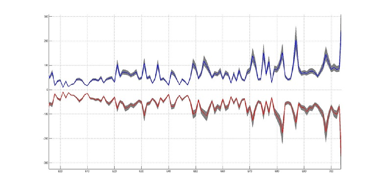
Figure 2 depicts the histogram of the number of buy order arrivals per a 15-second interval (left) and the same for sell order arrivals (right). It can be easily seen that these histograms are rather satisfactorily approximated by the GIG densities with the corresponding parameters. This is a good evidence in favor of the Cox process model proposed in this paper for the order counting processes. The explanation of such a good fit is given by lemma 5: if the expected intensity is high, then the asymptotic distribution of the mixed Poisson distribution is the same as that of the accumulated intensity. The corresponding intensities of the flows of buy and sell orders are shown on Fig. 3 where we again see a picture convincing that the multiplicativity representation for the intensities really holds. On Fig. 4 the graph of estimated (averaged over 60 sec) intensities imbalance process $r(t)$ is shown. It illustrates the general preponderance of buyers over sellers during the period of observation. Its deviations from the unit level are rather small.

So, as we have seen above, if $r(t)=r=\mathrm{const}$, then the OFI process can be successfully modeled by a generalized hyperbolic Lévy process with some parameters $a$, $\sigma$, $\nu$, $\mu$, $\lambda$. However, if the intensities imbalance process $r(t)$ is <<loosened>> and regarded as random, then the final adjustment of the model reduces to the account of that the parameters $a$, $\sigma$, $\nu$, $\mu$, $\lambda$ should be regarded as depending on $r(t)$, so that the final model looks like a a generalized hyperbolic Lévy process with random parameters. As this is so, in accordance with (35), the parameters $a(t)$ and $\sigma(t)$ accumulate the information concerning the current balance between the sizes and intensities of bid and ask orders, whereas in accordance with (34) the parameters $\nu(t)$, $\mu(t)$, $\lambda(t)$ are influenced only by the intensities imbalance $r(t)$. The prediction of the behavior of statistical regularities of this process and the corresponding risks reduces to the analysis of the trajectory of a point in a five-dimensional parametric space. For this purpose one can use multivariate autoregressive models.

References

- [1] Abergel F., Jedidi A. A mathematical approach to order book modelling // Econophysics of Order-Driven Markets / Abergel F., Chakrabarti B. K., Chakraborti A., Mitra M. (Eds.) Econophysics of Order-Driven Markets. – New York: Springer, 2011. P. 93–108.
- [2] Avellaneda M., Stoikov S. High-frequency trading in a limit order book // Quantitative Finance, 2008. Vol. 8. P. 217–224.
- [3] Barndorff-Nielsen O. E. Exponentially decreasing distributions for the logarithm of particle size // Proc. Roy. Soc. London. Ser. A, 1977. Vol. A(353). P. 401–419.
- [4] Barndorff-Nielsen O. E. Hyperbolic distributions and distributions of hyperbolae // Scand. J. Statist., 1978. Vol. 5. P. 151–157.
- [5] Barndorff-Nielsen O. E. Models for non-Gaussian variation, with applications to turbulence // Proc. Roy. Soc. London. Ser. A, 1979. Vol. A(368). P. 501–520.
- [6] Barndorff-Nielsen O. E., Kent J., Sørensen M. Normal variance-mean mixtures and z-distributions // International Statistical Review, 1982. Vol. 50. No. 2. P. 145–159.
- [7] Barndorff-Nielsen O. E. Processes of normal inverse Gaussian type // Finance and Stochastics, 1998. Vol. 2. P. 41–18.
- [8] Barndorff-Nielsen O. E., Mikosch T., Resnick S. I. Lévy Processes: Theory and Applications. – Boston: Birkhäuser, 2001.
- [9] Barndorff-Nielsen O. E., Blæsild P., Schmiegel J. A parsimonious and universal description of turbulent velocity increments // European Physical Journal, 2004. Vol. B. 41. P. 345–363.
- [10] Bening V., Korolev V. Generalized Poisson Models and Their Applications in Insurance and Finance. – Utrecht, VSP, 2002.
- [11] Bertoin J. Lévy Processes. Cambridge Tracts in Mathematics, Vol. 121. – Cambridge: Cambridge University Press, 1996.
- [12] Billingsley P. Convergence of Probability Measures. – New York: Wiley, 1968.
- [13] Bouchaud J.-P., Mezard M., Potters M. Statistical properties of stock order books: Empirical results and models // Quant. Finance, 2002. Vol. 2. P. 251-–256.
- [14] Carr P. P., Madan D. B., Chang E. C. The Variance Gamma process and option pricing // European Finance Review, 1998. Vol. 2. P. 79–105.
- [15] Chakraborti A., Toke I., Patriarca M., Abrergel F. Empirical facts and agent-based models // arXiv preprint arXiv:0909.1974, 2009.
- [16] Chertok A., Korolev V., Korchagin A., Shorgin S. Application of compound Cox processes in modeling order flows with non-homogeneous intensities // January 14, 2014. Available at SSRN: http://ssrn.com/abstract=2378975
- [17] Clark P. K. A subordinated stochastic process model with finite variance for speculative prices // Econometrica, 1973. Vol. 41. P. 135–155.
- [18] Cont R., Stoikov S., Talreja R. A stochastic model for order book dynamics // Operations Research, 2010. Vol. 58. No. 3. P. 549–563.
- [19] Cont R., de Larrard A. Order book dynamics in liquid markets: limit theorems and diffusion approximations // Working paper. Laboratoire de Probabilites et Modeles Aleatoires CNRS, Universite Pierre et Marie Curie (Paris VI) August 2011. Revised February 2012 (hal-00672274, version 2 – 1 October 2012).
- [20] Cont R., de Larrard A. Price dynamics in a Markovian limit order market. – Working paper, 2011. Available at: http://ssrn.com/abstract=1735338
- [21] Cont R., Kukanov A. and Stoikov S. The price impact of order book events // March 01, 2011. Available at SSRN: http://ssrn.com/abstract=1712822
- [22]
Cont R., Kukanov A. and Stoikov S. The price impact of order book
events,
Winter 2014, Journal of Financial Econometrics 12(1), pp. 47-88. - [23] Eberlein E., Keller U. Hyperbolic Distributions in Finance // Bernoulli, 1995. Vol. 1, No. 3. P. 281–299.
- [24] Eberlein E., Keller U., Prause K. New insights into smile, mispricing and value at risk: the hyperbolic model // Journal of Business, 1998. Vol. 71. P. 371–405.
- [25] Eberlein E., Prause K. The Generalized Hyperbolic Model: Financial Derivatives and Risk Measures. – Freiburg: Universität Freiburg, Institut für Mathematische Stochastic, 1998. Preprint No. 56.
- [26] Eberlein E. Application of Generalized Hyperbolic Lévy Motions to Finance. – Freiburg: Universität Freiburg, Institut für Mathematische Stochastic, 1999. Preprint No. 64.
- [27] Embrechts P., Maejima M. Selfsimilar Processes. – Princeton: Princeton University Press, 2002.
- [28] Foucault T. Order flow composition and trading costs in a dynamic limit order market // Journal of Financial Markets, 1999. Vol. 2. P. 99–134.
- [29] Geman H. Pure jump Lévy processes for asset price modelling // Journal of Banking and Finance, 2002. Vol. 26. No. 7. P. 1297–1316.
- [30] Gnedenko B. V., Fahim H. On a transfer theorem // Soviet Math. Dokl., 1969. Vol. 187. No. 1. P. 15–17.
- [31] Gnedenko B. V., Korolev V. Yu. Random Summation: Limit Theorems and Applications. – Boka Raton: CRC Press, 1996.
- [32] Goettler R., Parlour C., Rajan U. Equilibrium in a dynamic limit order market // Journal of Finance, 2005. Vol. 60. P. 2149–2192.
- [33] Grandell J. Doubly Stochastic Poisson Processes. Lecture Notes Mathematics, Vol. 529. – Berlin–Heidelberg–New York: Springer, 1976.
- [34] Granovsky B. L., Zeifman A. I. The decay function of nonhomogeneous birth and death processes, with application to mean-field models // Stochastic Process. Appl., 1997, Vol. 72. P. 105–120.
- [35] Huang H., Kercheval A. N. A generalized birth–death stochastic model for high-frequency order book dynamics // Quantitative Finance, 2012. Vol. 12. No. 4. P. 547–557.
- [36] Jacod J., Shiryaev A. N.. Limit theorems for stochastic processes. 2nd edition. Volume 288 of Grundlehren der Mathematischen Wissenschaften [Fundamental Principles of Mathematical Sciences]. – Berlin: Springer-Verlag, Berlin, 2003.
- [37] Kashcheev D. E. Modeling the Dynamics of Financial Time Series and Evaluation of Derivative Securities. PhD Thesis. – Tver: Tver State University, 2001 (in Russian).
- [38] Korolev V. Yu. Convergence of random sequences with the independent random indices. I // Theory Probab. Appl., 1994. Vol. 39. No. 2. P. 282–297.
- [39] Korolev V. Yu. On convergence of the distributions of random sums of independent random variables to stable laws // Theory Probab. Appl., 1997. Vol. 42. No. 4. P. 818–820.
- [40] Korolev V. Yu. On convergence of the distributions of compound Cox processes to stable laws // Theory Probab. Appl., 1998. Vol. 43. No. 4. P. 786–792.
- [41] Korolev V. Yu. Asymptotic properties of extrema of compound Cox processes and their application to some problems of financial mathematics // Theory Probab. Appl., 2000. Vol. 45. No. 1. P. 182–194.
- [42] Korolev V. Yu. Probabilistic and Statistical Methods For Decomposition of Volatility of Chaotic Processes. – Moscow: Moscow State University Publishing House, 2011 (in Russian).
- [43] Korolev V. Yu., Bening V. E., Shorgin S. Ya. Mathematical Foundation of Risk Theory. 2nd ed. – Moscow: FIZMATLIT, 2011 (in Russian).
- [44] Gorshenin A., Doynikov A., Korolev V., Kuzmin V. Statistical properties of the dynamics of order books: empirical results // Applied Problems in Theory of Probabilities and Mathematical Statistics Related to Modeling of Information Systems: Abstracts of VI International Workshop. – Moscow.: IPI RAS, 2012. P. 31–51.
- [45] Korolev V. Yu., Sokolov I. A. Skew Student distributions, variance gamma distributions and their generalizations as asymptotic approximations // Informatics and Its Applications, 2012. Vol. 6. No. 1. P. 2–10.
- [46] Zaks L. M., Korolev V. Yu. Generalized variance gamma distributions as limit laws for random sums // Informatics and Its Applications, 2013. Vol. 7. No. 1. P. 105–115.
- [47] Korolev V. Yu. Generalized hyperbolic laws as limit distributions for random sums // Theory of Probability and Its Applications, 2013. Vol. 58. No. 1. P. 117-–132.
- [48] Korolev V. Yu., Zaks L. M., Zeifman A. I. On convergence of random walks generated by compound Cox processes to Lévy processes // Statistics and Probability Letters, 2013. Vol. 83. No. 10. P. 2432–2438.
- [49] Korolev V. Yu., Chertok A. V., Korchagin A. Yu., Gorshenin A. K. Probabilistic and statistical modeling of information flows in complex financial systems from high-frequency data // Informatics and Its Applications, 2013. Vol. 7. No. 1. P. 12–21.
- [50] Chertok A. V., Korolev V. Yu., Zeifman A. I., Evstafiev A. I., Korchagin A. Yu., Shorgin S. Ya. Modeling stock order flows with non-homogeneous intensities from high-frequency data by two-sided risk processes. – Preprint. 2013.
- [51] Madan D. B., Seneta E. The variance gamma V.G. model for share market return // Journal of Business, 1990. Vol. 63. P. 511–524.
- [52] Mandelbrot B. B. Fractals and Scaling in Finance. Discontinuity, Concentration, Risk. – Berlin–Heidelberg: Springer, 1997.
- [53] Parlour Ch. A. Price dynamics in limit order markets // Rev. Financial Stud., 1998. Vol. 11. No. 4. P. 789–816.
- [54] Prause K. Modeling Financial Data Using Generalized Hyperbolic Distributions. – Freiburg: Universität Freiburg, Institut für Mathematische Stochastic, 1997. Preprint No. 48.
- [55] Rosu I. A dynamic model of the limit order book // Rev. Financial Stud., 2009. Vol. 22. P. 4601–4641.
- [56] Sato K. Lévy Processes and Infinitely Divisible Distributions. – Cambridge: Cambridge University Press, 1999.
- [57] Schoutens W. Lévy Processes in Finance: Pricing Financial Derivatives. – New York: Wiley, 2003.
- [58] Seshadri V. Halphen’s laws // Kotz, S., Read, C. B., Banks, D. L. (Eds.). Encyclopedia of Statistical Sciences, Update Volume 1. – New York: Wiley, 1997. P. 302–306.
- [59] Sichel H. S. Statistical evaluation of diamondiferous deposits // Journal of South Afr. Inst. Min. Metall., 1973. Vol. 76. P. 235–243.
- [60] Shiryaev A. N. Essentials of Stochastic Finance: Facts, Models, Theory. – Singapore: World Scientific. 1999.
- [61] Toke I. M. Market making in an order book model and its impact on the spread / In: Econophysics of Order-Driven Markets. New York – Berlin: Springer Verlag, 2011. P. 49-–64.
- [62] Zeifman A. I. Upper and lower bounds on the rate of convergence for nonhomogeneous birth and death processes // Stochastic Process. Appl., 1995. Vol. 59. P. 157–173.
- [63] Zolotarev V. M. One-Dimensional Stable Distributions. – Providence, R.I.: American Mathematical Society, 1986.
- [64] Zovko I., Farmer J. D. The power of patience; A behavioral regularity in limit order placement // Quant. Finance, 2002, Vol. 2. P. 387-–392.