Semi-Deterministic Broadcast Channels with Cooperation and a Dual Source Coding Problem

Abstract

The semi-deterministic broadcast channel (BC) where the decoders may cooperate via a finite-capacity one-sided link is considered. The capacity region is derived via a novel converse that uses a probabilistic construction of auxiliary random variables that depends on the distribution induced by the codebook. The BC is shown to be operationally equivalent to a certain class of relay-broadcast channels (RBCs) and the correspondence between their capacity regions is established. Furthermore, a source coding problem called the Ahlswede-Körner (AK) problem with one-sided encoder cooperation, is considered. Duality principles relating the two problems are presented and the optimal rate region for the source coding setting is derived. The best coding scheme incorporates several source coding techniques, such as Wyner-Ziv coding, binning and superposition coding. The capacity region of the semi-deterministic BC and the admissible region of the AK problem are shown to be dual to one another in the sense that the information measures defining the corner points of both regions coincide. Finally, several special cases of the BC setting and their capacity regions are inspected. It is shown that the special cases and their results preserve the dual relation to corresponding source coding problems.

I Introduction

Cooperation can dramatically boost the performance of a network. A common form of cooperation permits information exchange between the transmitting and receiving ends via rate-limited noise-free links, generally referred to as conferencing. This notion of cooperation was introduced by Williams in the context of a multiple-access channel (MAC), in which the encoders are able to hold a conference [1]. The Gaussian case was solved by Bross et al. in [2], followed by several works involving the compound MAC [3, 4]. Cooperation between receivers in a broadcast channel (BC) was introduced by Dabora and Servetto [5]. Liang and Veeravalli generalized the work in [5] by examining the problem of a relay-BC [6]. Both in [5] and [6] the capacity region of the physically degraded BC is characterized. The code construction combines superposition coding with the code construction for a degraded relay channel. In this paper we focus on a two-user semi-deterministic BC, in which the decoders cooperate via a rate-limited noise-free link, as illustrated in Fig. 1 and explained below.

Fig. 1: Semi-deterministic BC with one-sided decoder cooperation.

The semi-deterministic BC without cooperation was solved by Gelfand and Pinsker [7]. The coding scheme was based on Marton’s scheme for BCs [8]. Lapidoth and Wang extended the result in [7] to state-dependent channels where the state sequence is available at the encoder non-causally [9]. Thus, [9] extends the work by Gelfand and Pinker on the point-to-point (PTP) state-dependent channel with non-causal encoder channel state information (CSI) [10] to the semi-deterministic BC scenario. The converse proof in [9] included a new element: the choice of the auxiliary random variable was dependent on the codebook. The converse proof for the semi-deterministic BC with cooperation that is presented in this work generalizes the method used in [9].

In a standard converse proof, one identifies auxiliary random variables in a generic manner that suits all codebooks. However, such suitability is not required; rather, only an existence proof of appropriate random variables is required. The pursuit of auxiliaries that are optimal for all codebooks is an unnecessary restriction. Using this insight, we introduce a novel approach for converse proofs in which the auxiliary random variables are not only chosen as a function of the joint distribution induced by each codebook, but they are constructed in a probabilistic manner. In [9], the auxiliaries are deterministic functions of the joint distribution induced by the codebook. By allowing a probabilistic construction of the auxiliary random variables we introduce additional optimization parameters (i.e., a probability distribution). By doing so, an upper bound on the capacity region is tightened to coincide with the achievable region. Thus, our approach generalizes the manner in which converse proofs were treated until now, where the auxiliaries are chosen in a generic and deterministic manner. A probabilistic construction of a similar nature was used by Courtade and Weissman to characterize the admissible rate-distortion region for the multiterminal source coding problem under logarithmic loss [11]. The tightness of an inner bound on the region was derived by proving the existence of a joint distribution that satisfied appropriate fidelity constraints. The proof of existence relied on a probabilistic choice of random variables, however without explicitly stating the probability values that achieve optimality. In our case, a closed formula for these optimal values is derived as part of the converse proof. By exploiting the above technique, we establish a tight converse for the semi-deterministic BC with cooperation.

There is a close relation between the semi-deterministic BC with cooperation and a class of semi-deterministic relay-broadcast channels (RBCs) considered in [12] by Liang and Kramer. We show that a semi-deterministic RBC with an orthogonal and deterministic relay is operationally equivalent to the semi-deterministic BC considered in this work. In other words, a capacity achieving code for one problem also achieves the capacity of the other. Consequently, the capacity regions of the two problems are the same. However, there are several advantages to the approach taken in this work. First, we present a capacity achieving coding scheme over a single transmission block, while the scheme in [12] relies on transmitting many blocks and applying backward decoding. Thus, our scheme substantially reduces the delay introduced by backward decoding. Second, our converse results in a new characterization of the capacity region that gives insight into multiuser channel-source duality.

Fig. 2: The source coding problem considered.

To explore duality, we consider a source coding problem that we show is dual to the BC of interest. The setting is illustrated in Fig. 2 (see [13] and references therein for additional work involving cooperation in source coding problems). This setting is obtained from the BC by interchanging the roles of its encoder and decoders. Thus, the two problems are dual in a sense that naturally extends the well-known duality between PTP source and channel coding problems. PTP duality has been widely treated in the literature since it was studied by Shannon in 1948 and 1959 [14] (see [15, 16, 17] and references therein). The notion of duality in the context of multiuser settings, however, remains obscure even though it has attracted some attention in the last decade [18, 19, 13, 20]. We provide principles according to which the two problems can be transformed from one to the other. Moreover, upon deriving the optimal rate region for the source coding problem, we show that it is dual to the capacity region of the BC. The duality is in the sense that the information measures that define the corner points of both regions coincide, which is a natural extension of the relation between dual results in the PTP situation.

The source coding problem we consider is a special case of the two-encoder multiterminal source coding problem (cf., e.g., [21] and [22]). The optimal rate-distortion region for the latter setting remains one of the most challenging open problems in the field. Nonetheless, solutions for several special cases of the two-encoder source coding problem have been provided. Among these special cases are the Slepian-Wolf (SW) [23], Wyner-Ziv (WZ) [24], Gaussian quadratic [25] and Ahlswede-Körner (AK) [26] problems. The last setting refers to two correlated sources that are separately compressed, and their compressed versions are conveyed to the decoder which reproduces only one of the sources in a lossless manner. Considering the AK problem from the source coordination perspective forms the basis for the model that we focus on here.

Source coordination is an alternative formulation for lossy source coding. Strong coordination was considered by Wyner [27] while empirical coordination was studied in [28, 29, 30]. Cuff et al. extended these results to the multi-user case [31]. Rather than sending data from one point to another with a fidelity constraint, in a coordination problem all network nodes should develop certain joint statistics. Moreover, since achieving a distortion constraint is equivalent to reproducing sequences that admit a certain joint type, it was shown in [31] that rate-distortion theory is a special case of source coordination. In this work, we consider empirical coordination, a problem in which the terminals, upon observing correlated sources, generate sequences with a desired empirical joint distribution. An empirical coordination problem that is closely related to the source coding model of interest was presented by Bereyhi et al. [32], who considered a triangular multiterminal network. In this setting, each of the two terminals receives a different correlated source that it compresses and conveys to the decoder. The decoder outputs a sequence that achieves the desired coordination. Moreover, the encoders in [32] may share information via a one-sided cooperation link. The main contributions of [32] comprise inner and outer bounds on the optimal rate-region.

We derive a single-letter characterization of the coordination-capacity region of a special case of the triangular multiterminal network in [32]. We provide a coding scheme that unifies several concepts in source coding by relying on WZ coding [24], binning [33] and superposition coding [34]. The joint statistics of the output sequence is such that one of the sources can be reconstructed in a lossless manner from that output. Thus, this model can be regarded as an AK coordination problem with one-sided cooperative encoders. Note that in the classical AK problem, where the encoders are non-cooperative, the output sequence admits joint typicality with the side information even though this is not required. Since coordination is achieved by means of joint typicality of the sources and output with respect to the desired statistics, adding this typicality constraint to the original AK problem does not alter its solution. Indeed, under the proper assumptions, the rate region we give here reduces to the classical AK region. Berger and Yeung studied the case of the distributed source coding problem, i.e., where the encoders are non-cooperative, and one of the sources must be reproduced losslessly at the decoder [35]. They show that the quantize-and-bin scheme [25] is optimal. In [36], the authors showed that the scheme in [35] is suboptimal with a distortion constraint because it does not fully exploit the correlation between the sources.

This paper is organized as follows. In Section II we describe the two models of interest - the semi-deterministic BC with decoder cooperation and the AK problem with encoder cooperation. In Section III, we state capacity results for the BC and the AK models. Section V gives the converse for the semi-deterministic BC. The methodology used to prove the converse is elaborated. In Section VI the relation to a certain class of semi-deterministic RBCs is discussed. In Section IV we analyse the duality between the two problems of interest and their capacity regions. Section VII presents special cases of the capacity region of the semi-deterministic BC, and each case is shown to preserve a dual relation to the corresponding reduced source coding problem. Finally, Section VIII summarizes the main achievements and insights and suggests directions and extensions for further research.

II Preliminaries and Problem Definitions

We use the following notations. Calligraphic letters, e.g., $\mathcal{X}$, denote sets and the cardinality of a set $\mathcal{X}$ is denoted by $|\mathcal{X}|$. $\mathcal{X}^{n}$ stands for the $n$-fold Cartesian product of $\mathcal{X}$. An element of $\mathcal{X}^{n}$ is denoted by $x^{n}=(x_{1},x_{2},\ldots,x_{n})$, and its substrings as $x_{i}^{j}=(x_{i},x_{i+1},\ldots,x_{j})$, where $i\leq j$; when $i=1$, the subscript is omitted. We use the notation $x^{n\backslash i}=(x_{1},\ldots,x_{i-1},x_{i+1},\ldots,x_{n})$. Whenever the dimension $n$ is clear from the context, vectors (or sequences) are denoted by boldface letters, e.g., $\mathbf{x}$. Random variables are denoted by uppercase letter, e.g., $X$, with similar conventions for random vectors. $X_{i}^{j}$ stands for the sequence of random variables $(X_{i},X_{i+1},\ldots,X_{j})$, while $\mathbf{X}$ stands for $X^{n}$. The probability of an event $\mathcal{A}$ is denoted by $\mathbb{P}[\mathcal{A}]$, the indicator of $\mathcal{A}$ is dented by $\mathds{1}_{\mathcal{A}}$, while $\mathbb{P}[\mathcal{A}\big|\mathcal{B}\mspace{2mu}]$ stands for the conditional probability of $\mathcal{A}$ given $\mathcal{B}$. Probability mass functions (PMFs) are denoted by the capital letter $P$ with a subscript that identifies the random variable and its possible conditioning. For example, for two jointly distributed random variables $X$ and $Y$, let $P_{X}$, $P_{X,Y}$, and $P_{X|Y}$ denote, respectively, the PMF of $X$, the joint PMF of $(X,Y)$, and the conditional PMF of $X$ given $Y$. In particular, when $X$ and $Y$ are discrete, $P_{X|Y}$ represents the stochastic matrix whose elements are given by $P_{X|Y}(x|y)=\mathbb{P}\big[X=x|Y=y\big]$. We omit subscripts for notational simplicity whenever it is clear from the context.

II-A The Semi-Deterministic BC with One-Sided Decoder Cooperation

The $\big(\mathcal{X},\mathcal{Y}_{1},\mathcal{Y}_{2},\mathds{1}_{\{Y_{1}=f(X)\}}P_{Y_{2}|X}\big)$ semi-deterministic discrete memoryless broadcast channel (DMBC) with cooperation is illustrated in Fig. 1. The channel has one sender and two receivers. The sender chooses a pair $(m_{1},m_{2})$ of indices uniformly from the set $\left\{1,2,\ldots,2^{nR_{1}}\right\}\times\left\{1,2,\ldots,2^{nR_{2}}\right\}$; the choice of $m_{1}$ and $m_{2}$ is independent. The indices are mapped by the encoder to a sequence $x^{n}\in\mathcal{X}^{n}$, which is the channel input. The sequence $x^{n}$ is transmitted over the DMBC with transition probability $P_{Y_{1},Y_{2}|X}=\mathds{1}_{\{Y_{1}=f(X)\}}P_{Y_{2}|X}$. The output sequences $y_{1}^{n}\in\mathcal{Y}^{n}_{1}$ and $y_{2}^{n}\in\mathcal{Y}^{n}_{2}$ are received by decoder 1 and 2, respectively. Decoder $j\in\{1,2\}$ uses its available resources to produce an estimate of $m_{j}$; the estimate of $m_{j}$ is denoted by $\hat{m}_{j}$.

The channel is semi-deterministic in the sense $y_{1}=f(x)$, while $y_{2}$ is probabilistically drawn conditioned on $x$ according to the measure $P_{Y_{2}|X=x}$. A one-sided cooperation link of rate $R_{12}$ that extends from Decoder 1 to Decoder 2 is available. Accordingly, by conveying a cooperation message $m_{12}\in\{1,2,\ldots,2^{nR_{12}}\}$ over this link, Decoder 1 can share with Decoder 2 information about $y_{1}^{n}$, its decoded message $\hat{m}_{1}$, or both.

Definition 1 (Code Description)

A $(n,2^{nR_{12}},2^{nR_{1}},2^{nR_{2}})$ code for the semi-deterministic BC with one-sided decoder cooperation has:

1. Three message sets $\mathcal{M}_{12}=\{1,2,\ldots,2^{nR_{12}}\}$, $\mathcal{M}_{1}=\{1,2,\ldots,2^{nR_{1}}\}$ and $\mathcal{M}_{2}=\{1,2,\ldots,2^{nR_{2}}\}$.

2. An encoding function:

   $$g:\mathcal{M}_{1}\times\mathcal{M}_{2}\to\mathcal{X}^{n}.$$ (1a)

3. A decoder cooperation function:

   $$g_{12}:\mathcal{Y}_{1}^{n}\to\mathcal{M}_{12}.$$ (1b)

4. Two decoding functions:

   $$\psi_{1}:\mathcal{Y}_{1}^{n}\to\mathcal{M}_{1},$$ (1c)

   $$\psi_{2}:\mathcal{Y}_{2}^{n}\times\mathcal{M}_{12}\to\mathcal{M}_{2}.$$ (1d)

Definition 2 (Error Probability)

The average error probability for the $(n,2^{nR_{12}},2^{nR_{1}},2^{nR_{2}})$ code is

$$P_{e}^{(n)} =\mathbb{P}\Big[(\hat{M}_{1},\hat{M}_{2})\neq(M_{1},M_{2})\Big]=2^{-n(R_{1}+R_{2})}\mspace{-35mu}\sum_{(m_{1},m_{2})\in\mathcal{M}_{1}\times\mathcal{M}_{2}}\mspace{-25mu}\mathbb{P}\Big[\big(\hat{M}_{1},\hat{M}_{2}\big)\neq(m_{1},m_{2})\Big|(M_{1},M_{2})=(m_{1},m_{2})\Big].$$ (2a)

where $$\hat{M}_{1}=\psi_{1}(Y_{1}^{n}) \hat{M}_{2}=\psi_{2}(Y_{2}^{n},M_{12})$$ and . The average error probability for each receiver is defined by

$$P_{e,1}^{(n)}=\mathbb{P}\Big[\hat{M}_{1}\neq M_{1}\Big],$$ (2b)

$$P_{e,2}^{(n)}=\mathbb{P}\Big[\hat{M}_{2}\neq M_{2}\Big].$$ (2c)

A rate triple $(R_{12},R_{1},R_{2})$ is achievable if there is a sequence of $(n,2^{nR_{12}},2^{nR_{1}},2^{nR_{2}})$ codes with $P_{e}^{(n)}\rightarrow 0$ as $n\rightarrow\infty$. The capacity region is the closure of the set of the achievable rates.

II-B AK Source Coding Problem with One-Sided Encoder Cooperation

Consider the source coding problem illustrated in Fig. 2. Two source sequences $x_{1}^{n}\in\mathcal{X}_{1}^{n}$ and $x_{2}^{n}\in\mathcal{X}_{2}^{n}$ are available at Encoder 1 and Encoder 2, respectively. The sources are drawn in a pairwise independent and identically distributed (i.i.d.) manner according to the PMF $P_{X_{1},X_{2}}$. Each encoder communicates with the decoder by sending a message via a noiseless communication link of limited rate. The rate of the link between Encoder $i$ and the decoder is $R_{i}$ and the corresponding message is $T_{i}$, where $i\in\{1,2\}$. Moreover, Encoder 1 can communicate with Encoder 2 over a one-sided communication link of rate $R_{12}$.

Definition 3 (Coordination Code)

A $(n,2^{nR_{12}},2^{nR_{1}},2^{nR_{2}})$ coordination code for the AK coordination source coding problem with one-sided encoder cooperation has:

1. Three message sets: $\mathcal{T}_{12}=\{1,2,\ldots,2^{nR_{12}}\}$, $\mathcal{T}_{1}=\{1,2,\ldots,2^{nR_{1}}\}$ and $\mathcal{T}_{2}=\{1,2,\ldots,2^{nR_{2}}\}$.

2. An encoder cooperation function:

   $$f_{12}:\mathcal{X}_{1}^{n}\to\mathcal{T}_{12}.$$ (3a)

3. Two encoding functions:

   $$f_{1}:\mathcal{X}_{1}^{n}\to\mathcal{T}_{1},$$ (3b)

   $$f_{2}:\mathcal{X}_{2}^{n}\times\mathcal{T}_{12}\to\mathcal{T}_{2}.$$ (3c)

4. A decoding function:

   $$\phi:\mathcal{T}_{1}\times\mathcal{T}_{2}\to\mathcal{Y}^{n}.$$ (3d)

Definition 4 (Empirical Distribution)

The empirical distribution of $(x_{1}^{n},x_{2}^{n},y^{n})\in\mathcal{X}_{1}^{n}\times\mathcal{X}_{2}^{n}\times\mathcal{Y}^{n}$ is

$$\nu_{x_{1}^{n},x_{2}^{n},y^{n}}(a,b,c)\triangleq\frac{1}{n}\sum_{i=1}^{n}\mathds{1}_{\big\{(x_{1,i},x_{2,i},y_{i})=(a,b,c)\big\}}.$$ (4)

Definition 5 (Total Variation)

Let $P$ and $Q$ be two PMFs on $\mathcal{X}$. The total variation between $P$ and $Q$ is

$$||P-Q||_{TV}=\frac{1}{2}\sum_{a\in\mathcal{X}}\big|P(a)-Q(a)\big|.$$ (5)

Definition 6 (Coordination Achievability)

A distribution $P_{X_{2}}P_{Y|X_{2}}\mathds{1}_{\{X_{1}=f(Y)\}}$ is achievable with the rate triple $(R_{12},R_{1},R_{2})$ if there exists a sequence of coordination codes $(n,2^{nR_{12}},2^{nR_{1}},2^{nR_{2}})$ such that

$$\big|\big|\mspace{2mu}\nu_{X_{1}^{n},X_{2}^{n},Y^{n}}-P_{X_{2}}P_{Y|X_{2}}\mathds{1}_{\{X_{1}=f(Y)\}}\big|\big|_{TV}\underset{\mbox{\small{in probability}}}{\longrightarrow}0.$$ (6)

Definition 7 (Coordination Capacity Region)

The coordination capacity region is the closure of the set of all achievable rate triples $(R_{12},R_{1},R_{2})$ for a fixed desired distribution $P_{X_{2}}P_{Y|X_{2}}\mathds{1}_{\{X_{1}=f(Y)\}}$.

III Main Results

We state our main results as the capacity region for the semi-deterministic BC with cooperation (Subsection II-A) and the coordination capacity region for the AK coordination source coding problem (Subsection II-B).

Theorem 1 (Capacity Region of the Semi-Deterministic BC)

The capacity region of the semi-deterministic BC with one-sided encoder cooperation is the union of all sets of rate triples $(R_{12},R_{1},R_{2})\in\mathbb{R}^{3}_{+}$ satisfying:

$$R_{12} \geq I(V;Y_{1})-I(V;Y_{2})$$ (7a)

$$R_{1} \leq H(Y_{1})$$ (7b)

$$R_{2} \leq I(V,U;Y_{2})+R_{12}$$ (7c)

$$R_{1}+R_{2} \leq H(Y_{1}|V,U)+I(U;Y_{2}|V)+I(V;Y_{1})$$ (7d)

where the union is over all joint distributions $P_{V,U,Y_{1}}P_{X|V,U,Y_{1}}P_{Y_{2}|X}$ in which $Y_{1}=f(X)$. Moreover, $|\mathcal{V}|\leq|\mathcal{X}|+3$ and $|\mathcal{U}|\leq|\mathcal{V}|\cdot|\mathcal{X}|+1$.

The converse is established by using a novel technique that generalizes the classical approach. The existence of auxiliary random variables of the desired structure is demonstrated by constructing these auxiliaries in a probabilistic manner that depends on the joint distribution induced by each codebook. For the proof and an explanation of the new approach, see Section V. The proof of the direct part of Theorem 1 is given in Appendix  A.

The coordination capacity region of the AK problem with cooperation is stated next.

Theorem 2 (Coordination Capacity Region of the AK Problem)

The coordination capacity region of the AK coordination source coding problem with one-sided encoder cooperation for a desired coordination distribution $P_{X_{2}}P_{Y|X_{2}}\mathds{1}_{\{X_{1}=f(Y)\}}$ is the union of all sets of rate triples $(R_{12},R_{1},R_{2})\in\mathbb{R}^{3}_{+}$ satisfying:

$$R_{12} \geq I(V;X_{1}|X_{2})$$ (8a)

$$R_{1} \geq H(X_{1}|V,U)$$ (8b)

$$R_{2} \geq I(U;X_{2}|X_{1},V)$$ (8c)

$$R_{1}+R_{2} \geq H(X_{1}|V,U)+I(V,U;X_{1},X_{2})$$ (8d)

where the union is over all joint distributions $P_{X_{1},X_{2}}P_{V|X_{1}}P_{U|X_{2},V}P_{Y|X_{1},U,V}$ that have $P_{X_{2}}P_{Y|X_{2}}\mathds{1}_{\{X_{1}=f(Y)\}}$ as a marginal. Moreover, $|\mathcal{V}|\leq|\mathcal{X}_{1}|+4$ and $|\mathcal{U}|\leq|\mathcal{V}|\cdot|\mathcal{X}_{2}|+3$.

See Appendix C for the proof of Theorem 2.

Remark 3

The cardinality bounds on the auxiliary random variables $V$ and $U$ in Theorems 1 and 2 are established by invoking the support lemma [37, Lemma 15.4] twice. The details, being straightforward, are omitted.

Fig. 3: Corner points of the coordination capacity region of the AK coordination problem with cooperation at the hyperplane where $R_{12}=I(X_{1};V|X_{2})$.

Remark 4

For a fixed joint distribution in Theorem 2, the triples $(R_{12},R_{1},R_{2})$ at the corner points of the region defined by (8) are (see Fig. 3)

$$\big(\mspace{3mu}I(V;X_{1}|X_{2})\ ,\ H(X_{1})\ ,\ I(U;X_{2}|X_{1},V)\mspace{3mu}\big),$$ (9)

$$\big(\mspace{3mu}I(V;X_{1}|X_{2})\ ,\ H(X_{1}|V,U)\ ,\ I(U;X_{2}|V)+I(V;X_{1})\mspace{3mu}\big).$$ (10)

The corner point in (10) can be achieved using the coding scheme presented in [32] by setting $V=0$. However, it is not clear whether (9) is also achievable for that scheme.

Remark 5

The source coordination problem defined in Section II-B can be transformed into an equivalent rate-distortion problem. This is done by substituting $Y^{n}$, the output of the coordination problem, with the pair $(\hat{X}_{1}^{n},\hat{X}_{2}^{n})$, where $\hat{X}_{1}^{n}$ is a lossless reconstruction of the source sequence $X_{1}^{n}$, while $\hat{X}_{2}^{n}$ admits the distortion constraint

$$\mathbb{E}\Big[\sum_{i=1}^{n}d(X_{2,i},\hat{X}_{2,i})\Big]\leq D$$ (11)

where $d:\ \mathcal{X}_{2}\times\hat{\mathcal{X}}_{2}\to\mathbb{R}_{+}$ is a single letter distortion measure and $D\in\mathbb{R}_{+}$ is the distortion constraint. The two models are equivalent in the sense that the rate bounds that define the optimal rate regions of both problems admit the same forms; however, the domain over which the union is taken is slightly modified. This fact gives rise to the following corollary.

Corollary 6 (Rate Distortion Region of the AK Problem)

The achievable region for the equivalent rate-distortion problem is the union of all sets of rate triples $(R_{12},R_{1},R_{2})\in\mathbb{R}^{3}_{+}$ satisfying the bounds in (8), where the union is over all joint distributions $P_{X_{1},X_{2}}P_{V|X_{1}}P_{U|X_{2},V}$ and the reconstructions $\hat{X}_{2}$ that are deterministic functions of $(X_{1},U,V)$ such that $\mathbb{E}\big[d(X_{2},\hat{X}_{2})\big]\leq D$.

The proof of Corollary 6 is similar to that of Theorem 2 and is omitted.

Remark 7

The semi-deterministic BC with decoder cooperation and the AK problem with encoder cooperation are duals. A full discussion about the duality between the problems and their results is given in the following section.

IV Duality Between the Channel and Source Coding Problems

We examine the semi-deterministic BC with decoder cooperation (Fig. 1) and the AK coordination problem with encoder cooperation (Fig. 2) from the duality perspective. We show that the two problems and their solutions are dual to one another in a manner that naturally extends PTP duality [15, 16, 17]. In the PTP scenario, two channel and lossy source coding (or, equivalently, source coordination) problems are said to be dual if interchanging the roles of the encoder and the decoder in one problem produces the other. The solutions of these problems are dual in that they require an optimization of an information measure of the same structure, up to renaming the random variables involved. Solving one problem provides insight about the solution of the other. However, how duality extends to the multiuser case is still obscure.

In the context of multiuser lossy source coding, we favor the framework of source coordination over rate-distortion since the former provides a natural perspective on the similarities of the two problems. Source coordination inherently accounts for the probabilistic relations among all the sequences involved in the problem’s definition. However, in a coordination problem both the input and output (coordination) distributions are fixed, while in a channel coding problem the input distribution is optimized. Therefore, for convenience, throughout this section we consider channel codes with codewords of a fixed-type. This gives rise to the following definition (see also [13]).

Definition 8 (Fixed-Type Code Description, Achievability and Capacity Region)

A $(2^{nR_{12}},2^{nR_{1}},2^{nR_{2}},n,P_{X}^{\star})$ fixed-type code for the semi-deterministic BC with one-sided decoder cooperation consists of three integer sets and encoding, decoder cooperation and two decoding functions as defined in (4). For any $n\in\mathbb{N}$ and $\delta\geq 0$ we define the error probability as

$$P_{e}^{(n)}(\delta)=\mathbb{P}\bigg[\Big\{(\hat{M}_{1},\hat{M}_{2})\neq(M_{1},M_{2})\Big\}\bigcup\Big\{\big|\big|\nu_{X^{n},Y_{1}^{n},Y_{2}^{n}}-P_{X}^{\star}\mathds{1}_{\{Y_{1}=f(X)\}}P_{Y_{2}|X}\big|\big|_{TV}\geq\delta\Big\}\bigg],$$ (12)

where $p_{X^{n},Y_{1}^{n},Y_{2}^{n}}$ is the empirical distribution of the input and output sequences when averaged over all codebooks. The average error probability for each receiver is defined analogously. A rate triple $(R_{12},R_{1},R_{2})$ is achievable if for any $\delta>0$, there exists a sequence of codes such that $P_{e}^{(n)}(\delta)\to 0$ as $n\to\infty$. The definition of the corresponding capacity region is standard (see [38]).

Note that fixed-composition codes [39, 40, 41, 42] and codes that are drawn i.i.d. according to $P^{\star}_{X}$ satisfy the property in Definition 8. Moreover, the capacity region of the semi-deterministic BC with cooperation and a fixed-type code is similar to that stated in Theorem 1. The only difference between the two regions is the domain of joint distributions over which the union is taken. Specifically, for the BC with a fixed-type code, the union is taken over all joint distributions of the form $P_{V,U,Y_{1}}P_{X|V,U,Y_{1}}P_{Y_{2}|X}$ that have $P_{X}^{\star}\mathds{1}_{\{Y_{1}=f(X)\}}P_{Y_{2}|X}$ as a marginal.

TABLE I: Duality transformation principles: the AK problem with cooperation vs. the semi-deterministic BC with cooperation

Semi-Deterministic BC with Decoder Cooperation	AK Problem with Encoder Cooperation
Encoder inputs / Decoder outputs:	Decoder inputs / Encoder outputs:
$M_{i}\in\{1,2,...,2^{nR_{i}}\},$ $i\in\{1,2\}$	$T_{i}\in\{1,2,...,2^{nR_{i}}\},$ $i\in\{1,2\}$
Decoder inputs / Channel outputs:	Encoder inputs / Sources:
$Y_{1}^{n}\ ,\ Y_{2}^{n}$	$X_{1}^{n}\ ,\ X_{2}^{n}$
Encoder output / Channel input:	Decoder output / Coordination sequence:
$X^{n}$	$Y^{n}$
Encoding function:	Decoding functions:
$g:\mathcal{M}_{1}\times\mathcal{M}_{2}\rightarrow\mathcal{X}^{n}$	$\phi:\mathcal{T}_{1}\times\mathcal{T}_{2}\rightarrow\mathcal{Y}^{n}$
Decoder cooperation function:	Encoder cooperation functions:
$g_{12}:\mathcal{Y}_{1}^{n}\rightarrow\mathcal{M}_{12}$	$f_{12}:\mathcal{X}_{1}^{n}\rightarrow\mathcal{T}_{12}$
Decoding functions:	Encoding functions:
$\psi_{1}:\mathcal{Y}_{1}^{n}\to\mathcal{M}_{1}$,	$f_{1}:\mathcal{X}_{1}^{n}\to\mathcal{T}_{1}$,
$\psi_{2}:\mathcal{Y}_{2}^{n}\times\mathcal{M}_{12}\to\mathcal{M}_{2}$	$f_{2}:\mathcal{X}_{2}^{n}\times\mathcal{T}_{12}\to\mathcal{T}_{2}$

Note that each problem is obtained from the other by interchanging the roles of its encoder(s) and decoder(s) and renaming the random variables involved. A full description of the duality transformation principles is given in Table I. The duality is also evident in that the input and output sequences in both problems are jointly typical with respect to a joint PMF of the same form. Namely, in the channel coding problem, the triple $(x^{n},y_{1}^{n},y_{2}^{n})$ is jointly typical with high probability with respect to the joint PMF

$$P^{\star}_{X}\mathds{1}_{\{Y_{1}=f(X)\}}P_{Y_{2}|X}$$ (13)

where $P^{\star}_{X}$ is the code distribution. The corresponding triple of sequences $(x_{1}^{n},x_{2}^{n},y^{n})$ in the source coding problem is coordinated with respect to a joint PMF of the form

$$P_{X_{2}}P_{Y|X_{2}}\mathds{1}_{\{X_{1}=f(Y)\}}=P_{Y}\mathds{1}_{\{X_{1}=f(Y)\}}P_{X_{2}|Y}.$$ (14)

Therefore, by renaming the random variables according to Table I, the two PMFs in (13) and (14) coincide.

In fact, the duality between the two problems extends beyond the correspondence presented above. The capacity region of the BC stated in (7) and the coordination capacity region of the AK problem from (8) are also dual to one another. The corner points of the capacity region of the BC setting are

$$\big(\mspace{3mu}I(V;Y_{1})-I(V;Y_{2})\ ,\ H(Y_{1})\ ,\ I(U;Y_{2}|V)-I(U;Y_{1}|V)\mspace{3mu}\big)$$ (15)

$$\big(\mspace{3mu}I(V;Y_{1})-I(V;Y_{2})\ ,\ H(Y_{1}|V,U)\ ,\ I(U;Y_{2}|V)+I(V;Y_{1})\mspace{3mu}\big)$$ (16)

while the triple $(R_{12},R_{1},R_{2})$ at the corner points of the coordination-capacity region of the AK problem are

$$\big(\mspace{3mu}I(V;X_{1}|X_{2})\ ,\ H(X_{1})\ ,\ I(U;X_{2}|X_{1},V)\mspace{3mu}\big)$$ (17)

$$\big(\mspace{3mu}I(V;X_{1}|X_{2})\ ,\ H(X_{1}|V,U)\ ,\ I(U;X_{2}|V)+I(V;X_{1})\mspace{3mu}\big).$$ (18)

We show that (15)-(16) and (17)-(18) correspond by first rewriting the value of $R_{12}$ in (17)-(18) as

$$R_{12}=I(V;X_{1}|X_{1})\stackrel{{\scriptstyle(a)}}{{=}}I(V;X_{1})-I(V;X_{2})$$ (19)

where (a) follows from Markov relation $V-X_{1}-X_{2}$. Moreover, the value of $R_{2}$ in (17) is also rewritten as

$$R_{2}=I(U;X_{2}|X_{1},V)\stackrel{{\scriptstyle(a)}}{{=}}I(U;X_{2}|V)-I(U;X_{1}|V)$$ (20)

where (a) follows from the Markov relation $U-(X_{2},V)-X_{1}$.

Fig. 4: Corner point correspondence between: (a) the achievable rate region of the semi-deterministic BC with cooperation; (b) the coordination capacity region of the AK coordination problem with cooperation. The regions are depicted at their intersection with the hyperplanes of $(R_{1},R_{2})$ that correspond to $R_{12}=I(V;Y_{1})-I(V;Y_{2})$ and $R_{12}=I(V;X_{1})-I(V;X_{2})$, respectively.

By substituting (19)-(20) into (17)-(18) and renaming the random variables according to Table I, the corner points of both regions coincide (see Fig. 4).

Chronologically, upon observing the duality between the two problem settings, we solved the AK problem first. Then, based on past experience (cf., e.g., [13] and [20]), our focus turned to the dual semi-deterministic BC with cooperation. Since the capacity region is defined by the corner points of a union of polytopos, the structure of the capacity region for the semi-deterministic BC was evident. Thus, duality was key in obtaining the results of this work.

V Converse Proof for Theorem 1

The converse for Theorem 1 is established using a novel approach that generalizes the classical technique used for converse proofs. Our approach relies on two key properties. First, the construction of the auxiliary random variables depends on the joint distribution induced by the codebook. Second, the auxiliaries are constructed in a probabilistic manner.

We need to show that given an achievable rate triple $(R_{12},R_{1},R_{2})$, there exists a joint distribution of the form $P_{V,U,Y_{1}}P_{X|V,U,Y_{1}}P_{Y_{2}|X}$ in which $Y_{1}=f(X)$, such that the inequalities in (7) are satisfied. To do so, we first provide an upper bound on the region in (7) and then establish its inclusion in (7). The upper bound is stated in the following lemma.

Lemma 8 (Upper Bound on the Capacity Region)

Denote the region defined by the bounds in (7) by $\mathcal{C}$. Let $\mathcal{R}_{O}$ be the region defined by the union of all sets of rate triples $(R_{12},R_{1},R_{2})\in\mathbb{R}^{3}_{+}$ satisfying:

$$R_{12} \geq I(A;Y_{1}|C)-I(C;Y_{2}|A)$$ (21a)

$$R_{1} \leq H(Y_{1}|B,C)$$ (21b)

$$R_{2} \leq I(B;Y_{2}|A)+R_{12}$$ (21c)

$$R_{1}+R_{2} \leq H(Y_{1}|A,B,C)+I(B;Y_{2}|A,C)+I(A;Y_{1}|C)$$ (21d)

where the union is over all joint distributions $P_{A,B,C,Y_{1}}P_{X|A,B,C,Y_{1}}P_{Y_{2}|X}$ in which $Y_{1}=f(X)$. The following inclusion then holds:

$$\mathcal{C}\subseteq\mathcal{R}_{O}.$$ (22)

Proof:

Since $(R_{12},R_{1},R_{2})$ is achievable, there exists a sequence of $(n,2^{nR_{12}},2^{nR_{1}},2^{nR_{2}})$ codes for which $P_{e}^{(n)}\to 0$ as $n\to\infty$. By Fano’s inequality we have

$$H(M_{1}|Y_{1}^{n})\leq nR_{1}P_{e}^{(n)}+H\big(P_{e}^{(n)}\big)\triangleq n\epsilon_{n}^{(1)},$$ (23a)

$$H(M_{2}|M_{12},Y_{2}^{n})\leq nR_{2}P_{e}^{(n)}+H\big(P_{e}^{(n)}\big)\triangleq n\epsilon_{n}^{(2)},$$ (23b)

where $\epsilon_{n}^{(i)}\rightarrow 0$ as $P_{e}^{(n)}\rightarrow 0$ for $i\in\{1,2\}$. Define

$$\epsilon_{n}=\max_{i\in\{1,2\}}\big\{\epsilon_{n}^{(1)},\epsilon_{n}^{(2)}\big\}.$$ (24)

It follows that

$$nR_{12} \geq H(M_{12})$$

$$\stackrel{{\scriptstyle(a)}}{{=}}I(M_{12};Y_{1}^{n})$$

$$\stackrel{{\scriptstyle(b)}}{{=}}\sum_{i=1}^{n}\Big[I(M_{12},Y_{2,i+1}^{n};Y_{1}^{i})-I(M_{12},Y_{2,i}^{n};Y_{1}^{i-1})\Big]$$

$$\stackrel{{\scriptstyle(c)}}{{=}}\sum_{i=1}^{n}\Big[I(M_{12},Y_{2,i+1}^{n};Y_{1,i}|Y_{1}^{i-1})-I(Y_{1}^{i-1};Y_{2,i}|M_{12},Y_{2,i+1}^{n})\Big]$$

$$\stackrel{{\scriptstyle(d)}}{{=}}\sum_{i=1}^{n}\Big[I(A_{i};Y_{1,i}|C_{i})-I(C_{i};Y_{2,i}|A_{i})\Big]$$ (25)

where:
(a) follows because $M_{12}$ is a deterministic function of $Y_{1}^{n}$;
(b) follows from a telescoping identity [43, Equ. (9) and (11)];
(c) follows by the mutual information chain rule;
(d) follows by defining $A_{i}\triangleq(M_{12},Y_{2,i+1}^{n})$ and $C_{i}=Y_{1}^{i-1}$.

For the upper bound on $R_{1}$, consider

$$nR_{1} =H(M_{1})$$ (26)

$$=H(M_{1}|M_{2})$$

$$\stackrel{{\scriptstyle(a)}}{{\leq}}I(M_{1};Y_{1}^{n}|M_{2})+n\epsilon_{n}$$

$$\stackrel{{\scriptstyle(b)}}{{=}}H(Y_{1}^{n}|M_{2})-H(Y_{1}^{n}|M_{1},M_{2},X^{n})+n\epsilon_{n}$$ (27)

$$\stackrel{{\scriptstyle(c)}}{{=}}\sum_{i=1}^{n}H(Y_{1,i}|M_{2},Y_{1}^{i-1})+n\epsilon_{n}$$

$$\stackrel{{\scriptstyle(d)}}{{=}}\sum_{i=1}^{n}H(Y_{1,i}|B_{i},C_{i})+n\epsilon_{n}$$

where:
(a) follows from (23a) and (24);
(b) follows because $X^{n}$ is a deterministic function of $(M_{1},M_{2})$;
(c) follows because $Y_{1}^{n}$ is a deterministic function of $X^{n}$;
(d) follows by defining $B_{i}\triangleq M_{2}$ and from the definition of $C_{i}$.

Next, to bound $R_{2}$ we have

$$nR_{2} =H(M_{2})$$ (28)

$$\stackrel{{\scriptstyle(a)}}{{\leq}}I(M_{2};M_{12},Y_{2}^{n})+n\epsilon_{n}$$

$$=I(M_{2};Y_{2}^{n}|M_{12})+I(M_{2};M_{12})+n\epsilon_{n}$$ (29)

$$\leq\sum_{i=1}^{n}I(M_{2};Y_{2,i}|M_{12},Y_{2,i+1}^{n})+H(M_{12})+n\epsilon_{n}$$

$$\stackrel{{\scriptstyle(b)}}{{\leq}}\sum_{i=1}^{n}I(B_{i};Y_{2,i}|A_{i})+nR_{12})+n\epsilon_{n}$$ (30)

where (a) follows from (23b) and (24), while (b) follows from the definition of $(A_{i},B_{i})$ and because a uniform distribution maximizes entropy.

Finally, for the sum of rates, we begin by writing

$$n(R_{1}+R_{2})=H(M_{1},M_{2})=H(M_{2})+H(M_{1}|M_{2}).$$ (31)

By repeating steps (26)-(27) we have

$$H(M_{1}|M_{2})\leq H(Y_{1}^{n}|M_{2})+n\epsilon_{n}.$$ (32)

Next, consider

$$H(M_{2}) \stackrel{{\scriptstyle(a)}}{{\leq}}I(M_{2};Y_{2}^{n}|M_{12})+I(M_{2};M_{12})+n\epsilon_{n}$$

$$\stackrel{{\scriptstyle(b)}}{{=}}\sum_{i=1}^{n}\Big[I(M_{2};Y_{2,i}^{n}|M_{12},Y_{1}^{i-1})-I(M_{2};Y_{2,i+1}^{n}|M_{12},Y_{1}^{i})\Big]+I(M_{2};M_{12})+n\epsilon_{n}$$

$$\begin{multlined}\stackrel{{\scriptstyle(c)}}{{=}}\sum_{i=1}^{n}\Big[I(M_{2};Y_{2,i+1}^{n}|M_{12},Y_{1}^{i-1})+I(B_{i};Y_{2,i}|A_{i},C_{i})-I(M_{2};Y_{1,i},Y_{2,i+1}^{n}|M_{12},Y_{1}^{i-1})\\ +I(M_{2};Y_{1,i}|M_{12},Y_{1}^{i-1})\Big]+I(M_{2};M_{12})+n\epsilon_{n}\end{multlined}$$

$$\begin{multlined}\stackrel{{\scriptstyle(d)}}{{=}}\sum_{i=1}^{n}\Big[I(B_{i};Y_{2,i}|A_{i},C_{i})-I(M_{2};Y_{1,i}|M_{12},Y_{1}^{i-1},Y_{2,i+1}^{n})\Big]+I(M_{2};M_{12},Y_{1}^{n})+n\epsilon_{n}\end{multlined}$$

$$\begin{multlined}\stackrel{{\scriptstyle(e)}}{{=}}\sum_{i=1}^{n}\Big[H(Y_{1,i}|A_{i},B_{i},C_{i})+I(B_{i};Y_{2,i}|A_{i},C_{i})-H(Y_{1,i}|M_{12},Y_{1}^{i-1},Y_{2,i+1}^{n})\Big]+I(M_{2};Y_{1}^{n})+n\epsilon_{n}\end{multlined}$$ (33)

where:
(a) follows from repeating steps (28)-(29) in the upper bounding of $R_{2}$;
(b) follows from a telescoping identity [43, Equ. (9) and (11)];
(c) follows from the definition of $(A_{i},B_{i},C_{i})$;
(d) follows for the mutual information chain rule;
(e) follows from the definition of $(A_{i},B_{i},C_{i})$ (first term) and from the Markov relation $M_{12}-Y_{1}^{n}-M_{2}$ (fourth term).

By substituting (32) and (33) into (31), we obtain

$$n(R_{1}+R_{2}) \leq\sum_{i=1}^{n}\Big[H(Y_{1,i}|A_{i},B_{i},C_{i})+I(B_{i};Y_{2,i}|A_{i},C_{i})-H(Y_{1,i}|M_{12},Y_{1}^{i-1},Y_{2,i+1}^{n})\Big]+H(Y_{1}^{n})+2n\epsilon_{n}$$

$$\stackrel{{\scriptstyle(a)}}{{=}}\sum_{i=1}^{n}\Big[H(Y_{1,i}|A_{i},B_{i},C_{i})+I(B_{i};Y_{2,i}|A_{i},C_{i})+I(A_{i};Y_{1,i}|C_{i})\Big]+2n\epsilon_{n}$$ (34)

where (a) follows from the mutual information chain rule and the definition of $(A_{i},B_{i},C_{i})$.

The upper bounds in (25), (27), (30) and (34) can be rewritten by introducing a time sharing random variable $Q$ that is uniformly distributed over the set $\{1,2,...,n\}$. The upper bound in (25) can then be rewritten as

$$R_{12} \geq\frac{1}{n}\sum_{i=1}^{n}\Big[I(A_{i};Y_{1,i}|C_{i})-I(C_{i};Y_{2,i}|A_{i})\Big]$$

$$=\sum_{i=1}^{n}\mathbb{P}\big[Q=i\big]\Big[I(A_{Q};Y_{1,Q}|C_{Q},Q=i)-I(C_{Q};Y_{2,Q}|A_{Q},Q=i)\Big]$$

$$=I(A_{Q};Y_{1,Q}|C_{Q},Q)-I(C_{Q};Y_{2,Q}|A_{Q},Q).$$ (35)

By rewriting the rate bounds (27), (30) and (34) in the same manner, the region obtained is convex. This follows from the presence of the time sharing random variable $Q$ in the conditioning of all the mutual information terms.

Next, let $Y_{1}\triangleq Y_{1,Q},\ Y_{2}\triangleq Y_{2,Q},\ A\triangleq(A_{Q},Q),\ B\triangleq B_{Q}$ and $C\triangleq(C_{Q},Q)$. We have

$$R_{12} \geq I(A;Y_{1}|C)-I(C;Y_{2}|A)$$ (36a)

$$R_{1} \leq H(Y_{1}|B,C)+\epsilon_{n}$$ (36b)

$$R_{2} \leq I(B;Y_{2}|A)+R_{12}+\epsilon_{n}$$ (36c)

$$R_{1}+R_{2} \leq H(Y_{1}|A,B,C)+I(B;Y_{2}|A,C)+I(A;Y_{1}|C)+2\epsilon_{n}.$$ (36d)

Note that the auxiliary random variables $(A,B,C)$ admit the Markov relation

$$(Y_{1},Y_{2})-X-(A,B,C)$$ (37)

due to the deterministic and the memoryless property of the channel and since the channel is without feedback. By taking the limit as $P_{e}^{(n)}\rightarrow 0$, we obtain the rate bounds (21). Thus, we obtain that $\mathcal{C}\subseteq\mathcal{R}_{2}$. ∎

Using the upper bound in Lemma 8, the converse is completed by the following lemma.

Lemma 9 (Tightness of the Upper Bound)

The following inclusion relation holds:

$$\mathcal{R}_{O}\subseteq\mathcal{C}.$$ (38)

Proof:

Let $(R_{12},R_{1},R_{2})\in\mathcal{R}_{O}$ be achieved by a given tuple of random variables $(A,B,C,X)$. We show that there exists a pair of random variables $(V,U)$ such that $(R_{12},R_{1},R_{2})\in\mathcal{C}$ is achieved by $(V,U,X)$. We define $(V,U)$ as follows. Let $\Theta\sim\mbox{Ber}\left(\lambda\right)$, $\lambda\in[0,1]$, be a binary random variable independent of $(A,B,C,X)$ that takes values in $\mathcal{O}=\{\theta_{1},\theta_{2}\}$. Define the random variable

$$\widetilde{V}=\begin{cases}(A,C)\ ,&\Theta=\theta_{1}\\ \emptyset\ ,&\Theta=\theta_{2}\end{cases}.$$ (39)

The auxiliary random variable $V$ is defined as $V\triangleq(\Theta,\widetilde{V})$. Furthermore, define

$$U=(A,B,C)$$ (40)

and note that $(V,U)$ preserves the Markov structure

$$(Y_{1},Y_{2})-X-(U,V)$$ (41)

by (37). We further have

$$I(V;Y_{1})-I(V;Y_{2}) =\lambda\Big[I(A,C;Y_{1})-I(A,C;Y_{2})\Big]$$ (42)

$$=\lambda\Big[I(A;Y_{1}|C)-I(A,C;Y_{2})+I(C;Y_{1})\Big]$$ (43)

$$\stackrel{{\scriptstyle(a)}}{{\leq}}I(A;Y_{1}|C)-I(C;Y_{2}|A)\stackrel{{\scriptstyle(b)}}{{\leq}}R_{12}$$ (44)

where (a) follows by taking

$$\lambda=\min\Bigg\{1,\bigg(\frac{I(A;Y_{1}|C)-I(A,C;Y_{2})+I(A;Y_{2})}{I(A;Y_{1}|C)-I(A,C;Y_{2})+I(C;Y_{1})}\bigg)^{+}\Bigg\}$$ (45)

where $(x)^{+}=\max\big\{0,x\big\}$, and (b) follows from (21a). Inequality (a) in (44) is proved as follows. First, if $\lambda=1$ we have

$$I(A;Y_{2})\geq I(C;Y_{1}).$$ (46)

The term in (43) can then be rewritten as

$$\lambda\Big[I(A;Y_{1}|C)-I(A,C;Y_{2})+I(C;Y_{1})\Big] \stackrel{{\scriptstyle(a)}}{{=}}I(A;Y_{1}|C)-I(C;Y_{2}|A)+I(C;Y_{1})-I(A;Y_{2})$$

$$\stackrel{{\scriptstyle(b)}}{{\leq}}I(A;Y_{1}|C)-I(C;Y_{2}|A)$$

where (a) follows using $\lambda=1$ and the mutual information chain rule, while (b) follows from (46). On the other hand, if

$$\lambda=\frac{I(A;Y_{1}|C)-I(A,C;Y_{2})+I(A;Y_{2})}{I(A;Y_{1}|C)-I(A,C;Y_{2})+I(C;Y_{1})}$$ (47)

then

$$I(A;Y_{2})<I(C;Y_{1})$$ (48)

and we rewrite (43) as

$$\lambda\Big[I(A;Y_{1}|C)-I(A,C;Y_{2})+I(C;Y_{1})\Big] \stackrel{{\scriptstyle(a)}}{{=}}I(A;Y_{1}|C)-I(A,C;Y_{2})+I(A;Y_{2})$$

$$=I(A;Y_{1}|C)-I(C;Y_{2}|A).$$

Here (a) follows from (47). The case $\lambda=0$ is trivial, and we omit the derivation of (a) in (44). We conclude that (7a) is satisfied. (7b) is implied because $H(Y_{1}|B,C)\leq H(Y_{1})$.

We proceed with deriving (7c). First note that the definition of $(V,U)$ in (39)-(40) implies

$$(A,B,C,X,Y_{1},Y_{2})-U-V.$$ (49)

Consequently, we obtain

$$I(V,U;Y_{2})=I(A,B,C;Y_{2})$$ (50)

which yields

$$I(V,U;Y_{2})+R_{12}\stackrel{{\scriptstyle(a)}}{{=}}I(A,C,B;Y_{2})+R_{12}\geq I(B;Y_{2}|A)+R_{12}\stackrel{{\scriptstyle(b)}}{{\geq}}R_{2}.$$ (51)

Inequality (a) in (51) follows from (40) and (49), while (b) follows from (21c). This shows that (7c) also holds.

Finally, for the sum rate we begin by rewriting (7d) as

$$H(Y_{1}|V,U)+I(U;Y_{2}|V)+I(V;Y_{1})=H(Y_{1}|V,U)+I(V,U;Y_{2})+I(V;Y_{1})-I(V;Y_{2}).$$ (52)

Next, we obtain an explicit expression for each of the information measures in the right-hand side (RHS) of (52) in terms of $(A,B,C,X)$. Based on similar arguments to those presented before, we have

$$H(Y_{1}|V,U)=H(Y_{1}|A,B,C)$$ (53)

while the other two information measures in (52) were previously evaluated in (42) and (50). Thus, by substituting (42), (50) and (53) into (52), we obtain

$$H(Y_{1}|V,U)+I(U;Y_{2}|V)+I(V;Y_{1}) =H(Y_{1}|A,B,C)+I(A,B,C;Y_{2})+\lambda\Big[I(A,C;Y_{1})-I(A,C;Y_{2})\Big]$$

$$\stackrel{{\scriptstyle(a)}}{{\geq}}H(Y_{1}|A,B,C)+I(B;Y_{2}|A,C)+I(A;Y_{1}|C)\stackrel{{\scriptstyle(b)}}{{\geq}}R_{1}+R_{2}$$ (54)

where (a) follows from the choice of $\lambda$ in (45), while (b) follows by (21d).

The derivation of (a) in (54) relies on evaluating the terms of interest for two cases of $\lambda$. For $\lambda=1$ and using the mutual information chain rule we have

$$H(Y_{1}|V,U)+I(U;Y_{2}|V)+I(V;Y_{1}) =H(Y_{1}|A,B,C)+I(B;Y_{2}|A,C)+I(A,C;Y_{1})$$

$$\geq H(Y_{1}|A,B,C)+I(B;Y_{2}|A,C)+I(A;Y_{1}|C).$$ (55)

On the other hand, if $\lambda$ satisfies (47) we obtain

$$H(Y_{1}|V,U)+I(U;Y_{2}|V)+I(V;Y_{1}) =H(Y_{1}|A,B,C)+I(A;Y_{2})+I(B;Y_{2}|A,C)+I(A;Y_{1}|C)$$

$$\geq H(Y_{1}|A,B,C)+I(B;Y_{2}|A,C)+I(A;Y_{1}|C).$$ (56)

Thus, (7d) is also satisfied. Concluding, since all the rate bounds in (7) hold for the choice of $(V,U)$ stated in (39)-(40), we get $(R_{12},R_{1},R_{2})\in\mathcal{C}$, which implies the inclusion $\mathcal{R}_{O}\subseteq\mathcal{C}$.

∎

Lemma 9 completes the converse and characterizes the region in (7) as the capacity region of the semi-deterministic BC with cooperation.

Remark 10

The definition of $V$ in (39) is probabilistic and depends on the joint distribution of $(A,B,C,X)$ that is induced by the codebook. More specifically, the choice of $\lambda$ in (45) varies with each joint distribution and is chosen to yield the inclusion (38).

Remark 11

As shown in the direct part of the proof (see Appendix A), the cooperation scheme employed by Decoder 1 is based on a WZ-like coding. Namely, $Y_{1}^{n}$ is viewed as the source to be compressed, while $Y_{2}^{n}$ is the correlated side information. The choice of $V$ in (39) as $(A,C)$ (with probability $\lambda$) is consistent with the auxiliary random variable in the converse proof for the classical WZ setting by recalling that $A_{i}\triangleq(M_{12},Y_{2,i+1}^{n})$ and $C_{i}=Y_{1}^{i-1}$.

VI Relation to the Semi-Deterministic Relay Broadcast Channel

Fig. 5: General RBC.

The semi-deterministic BC with cooperation is strongly related to the semi-deterministic RBC that was studied in [12]. In this section we show that under proper assumptions the two models are operationally equivalent.

A general RBC is illustrated in Fig. 5 (for the full definition see [12, Section II]). The RBC is semi-deterministic if the probability distribution $P_{Y_{1}|X,X_{1}}$ takes only on the values 0 or 1. To see the correspondence between the semi-deterministic RBC and the BC of interest, let $Y_{2}=(Y_{21},Y_{22})$ and let the channel transition distribution factorize as

$$P_{Y_{1},Y_{21},Y_{22}|X,X_{1}}=P_{Y_{21}|X}\mathds{1}_{\{Y_{1}=f(X)\}}P_{Y_{22}|X_{1}}.$$ (57)

(57) implies that the channel from the encoder to the decoders is orthogonal to the one between the decoders. Suppose the relay channel is deterministic with capacity $R_{12}$ and let $Y_{22}=f_{R}(X_{1})$. As stated in the following lemma, the reduced semi-deterministic RBC that is obtained under these assumptions is operationally equivalent to the semi-deterministic BC with cooperation.

Lemma 12 (Operational Equivalence)

For every reduced semi-deterministic RBC (with respect to the above assumptions) there is a semi-deterministic BC with cooperation such that a capacity achieving code for the former also achieves the capacity of the latter, and vise versa.

Proof:

Suppose that $\Big\{\mathcal{C}_{RBC}^{(n)}\Big\}_{n=1}^{\infty}$ is a capacity achieving sequence of $(n,2^{nR_{1}},2^{nR_{2}})$ codes for a reduced semi-deterministic RBC. Since the channel from Decoder 1 to Decoder 2 is deterministic, there are approximately $2^{nH(Y_{22})}$ different possible relay channel outputs $\mathbf{y}_{22}$. For every sequence $\mathbf{y}_{22}\in\mathcal{T}_{\epsilon}^{(n)}(Y_{22})$ (here $\epsilon>0$ corresponds to the margin between the region achieved by the $n$th code and the capacity region) define the following subset of $\mathbf{x}_{1}$ codewords:

$$\mathcal{V}(\mathbf{y}_{22})=\Big\{\mathbf{x}_{1}\in\mathcal{C}_{RBC}\ \Big|\ f_{R}(x_{1,i})=y_{22,i},\ \forall i\in\{1,\ldots,n\}\Big\}.$$ (58)

Consider a semi-deterministic BC with cooperation link capacity of approximately $2^{nH(Y_{22})}$ and associate a cooperation message $m_{12}$, where $m_{12}\in\{1,\ldots,2^{nH(Y_{22})}\}$, with every set $\mathcal{V}(\mathbf{y}_{22})$. To use $\mathcal{C}_{RBC}^{(n)}$ for the semi-deterministic BC with cooperation, Decoder 1 waits for the $n$-symbol transmission to end and then shares with Decoder 2 the message $m_{12}$ associated with a set $\mathcal{V}(\mathbf{y}_{22})$ that contains the intended $\mathbf{x}_{1}$ codeword (i.e., such that $\mathbf{x}_{1}\in\mathcal{V}(\mathbf{y}_{22})$). Upon receiving $m_{12}$, Decoder 2 recovers the sequence $\mathbf{y}_{22}$ and proceeds with the decoding process of the RBC coding scheme. Thus, the coding scheme for the semi-deterministic RBC, using the sequence of codes $\Big\{\mathcal{C}_{RBC}^{(n)}\Big\}_{n=1}^{\infty}$, achieves capacity for the semi-deterministic BC with cooperation.

Next, suppose that $\Big\{\mathcal{C}_{BCC}^{(n)}\Big\}_{n=1}^{\infty}$ is a sequence of $(n,2^{nR_{12}},2^{nR_{1}},2^{nR_{2}})$ capacity achieving codes for a semi-deterministic BC with cooperation. Consider a RBC with relay capacity $R_{12}$ and map each cooperation message $m_{12}\in\{1,\ldots,2^{nR_{12}}\}$ to a codeword $\mathbf{x}_{1}(m_{12})$. Since the capacity of the channel between the decoders is large enough there is a sufficient number of different codewords $\mathbf{x}_{1}$ (i.e., sufficient to cover the space of cooperation messages $\{1,\ldots,2^{nR_{12}}\}$) that can be conveyed via this channel. To use $\mathcal{C}_{BCC}^{(n)}$ for the semi-deterministic RBC we transmit $B$ blocks, each of length $n$, and denote the messages transmitted by $(m_{1}^{(b)},m_{2}^{(b)})\in\mathcal{M}_{1}\times\mathcal{M}_{2}$, where $b\in\{1,\ldots,B\}$. In the subsequent coding scheme, the transmission of the 1st block is disregarded, while during every block $b\geq 2$, the messages $(m_{1}^{(b-1)},m_{2}^{(b-1)})$ are reliably transmitted over the channel. Accordingly, the scheme forfeits the decoding of the messages $(m_{1}^{(B)},m_{2}^{(B)})$, which implies that the average rate pair $\left(\frac{B-1}{B}R_{1},\frac{B-1}{B}R_{2}\right)$, over $B$ blocks, is achievable. By taking $B\to\infty$, the transmission rates approach $(R_{1},R_{2})$.

The coding scheme for the semi-deterministic RBC during block $b\geq 2$ is described subsequently. First note that the channel output $\mathbf{y}_{1}^{(b-1)}$ at Decoder 1 during the previous block is known at the relay at the beginning of block $b$. Thus, during block $b$, the encoder transmits the codeword $\mathbf{x}$ that corresponds to the message pair $(m_{1}^{(b-1)},m_{2}^{(b-1)})$, while the relay transmits the codeword $\mathbf{x}_{1}\Big(m_{12}^{(b-1)}\big(\mathbf{y}_{1}^{(b-1)}\big)\Big)$. At the end of transmission block $b$, Decoder 2 uses the induced relay output $\mathbf{y}_{22}^{(b)}$ to reliably decode $m_{12}^{(b-1)}\big(\mathbf{y}_{1}^{(b-1)}\big)$. Both decoders then proceed with the decoding process for the semi-deterministic BC with cooperation to decode the messages $(m_{1}^{(b-1)},m_{1}^{(b-1)})$. Taking $B$ and and $n$ to infinity, the coding scheme for the semi-deterministic BC with cooperation achieves capacity for the semi-deterministic RBC. ∎

Due to the equivalence of the two models their capacity regions also coincide. If the orthogonal and deterministic relay channel has capacity $R_{12}$, the capacity region for the semi-deterministic RBC (stated in Theorem 8 in [12]) is the union of all sets of rate pairs $(R_{1},R_{2})\in\mathbb{R}^{2}_{+}$ satisfying:

$$R_{1} \leq H(Y_{1}|X_{1})$$ (59a)

$$R_{2} \leq I(V,U,X_{1};Y_{21})+H(Y_{22}|Y_{21})$$ (59b)

$$R_{1}+R_{2} \leq H(Y_{1}|V,U,X_{1})+I(U;Y_{21}|V,X_{1})+I(V;Y_{1}|X_{1})$$ (59c)

$$R_{1}+R_{2} \leq H(Y_{1}|V,U,X_{1})+I(V,U,X_{1};Y_{21})+H(Y_{22}|Y_{21})$$ (59d)

where the union is over all joint distributions $P_{V,U,X,X_{1}}P_{Y_{21}|X}\mathds{1}_{\{Y_{1}=f(X)\}}\mathds{1}_{\{Y_{22}=f_{R}(X_{1})\}}$.

In Appendix D we demonstrate that the region given in (59) can be simplified to

$$R_{1} \leq H(Y_{1})$$ (60a)

$$R_{2} \leq I(V,U;Y_{21})+R_{12}$$ (60b)

$$R_{1}+R_{2} \leq H(Y_{1}|V,U)+I(U;Y_{21}|V)+I(V;Y_{1})$$ (60c)

$$R_{1}+R_{2} \leq H(Y_{1}|V,U)+I(V,U;Y_{21})+R_{12}$$ (60d)

where the union is over all joint distributions $P_{V,U,X}P_{X_{1}}P_{Y_{21}|X}\mathds{1}_{\{Y_{1}=f(X)\}}\mathds{1}_{\{Y_{22}=f_{R}(X_{1})\}}$. In Appendix E we establish that the region characterized by (60) coincides with the capacity region of the semi-deterministic BC with cooperation stated in Theorem 1.

The advantage of the approach taken in this work compared to [12] is twofold. First, we achieve capacity over a single transmission block, while the scheme in [12] transmits a large number of blocks and applies backward decoding. The substantial delay introduced by a backward decoding process implies the superiority of our scheme for practical uses. Consequently, the two coding schemes induce different characterizations of the capacity region. The difference is expressed in replacing the lower bound on $R_{12}$ in (7a) with the additional bound on the sum rate stated in (60d). Due to the particular structure of the region in (7), which involves the lower bound on the cooperation rate $R_{12}$, our approach for the converse proof is essential to establish optimality. The second advantage is the correspondence between the obtained capacity region for the semi-deterministic BC with cooperation and the coordination-capacity region of the dual AK source coding problem. This duality is presented and discussed in Section IV, and it yields insight into the relation between channel and source coding problems.

VII Special Cases

We consider special cases of the capacity region of the semi-deterministic BC with decoder cooperation and show that the dual relation discussed in Section IV is preserved for each special case.

VII-A The Fully-Deterministic BC with Decoder Cooperation

Corollary 13 (Capacity Region of the Fully-Deterministic BC)

The capacity region of a fully-deterministic BC is the union of all sets of rate triples $(R_{12},R_{1},R_{2})\in\mathbb{R}^{3}_{+}$ satisfying:

$$R_{1} \leq H(Y_{1})$$ (61a)

$$R_{2} \leq H(Y_{2})+R_{12}$$ (61b)

$$R_{1}+R_{2} \leq H(Y_{1},Y_{2})$$ (61c)

where the union is over all input distributions $P_{X}$.

Proof:

Achievability follows from Theorem 1 by taking $V=0$ and $U=Y_{2}$. A converse for (61) is easily established as follows. Consider the bounds:

$$R_{12} \geq I(V;Y_{1})-I(V;Y_{2})\geq 0,$$

$$R_{2} \leq I(V,U;Y_{2})+R_{12}\leq H(Y_{2})+R_{12}$$

and

$$R_{1}+R_{2} \leq H(Y_{1}|V,U)+I(U;Y_{2}|V)+I(V;Y_{1})$$

$$=H(Y_{1})+I(U;Y_{2}|V)-I(U;Y_{1}|V)$$

$$=H(Y_{1})-H(U|V,Y_{2})+H(U|V,Y_{1})$$

$$\leq H(Y_{1})-H(U|V,Y_{1},Y_{2})+H(U|V,Y_{1})$$

$$=H(Y_{1})+I(U;Y_{2}|V,Y_{1})$$

$$\leq H(Y_{1})+H(Y_{2}|V,Y_{1})\leq H(Y_{1},Y_{2}).$$

(61) is thus the capacity region of the deterministic BC with one-sided decoder cooperation. ∎

The fully-deterministic BC is dual to the SW source coding problem with one-sided encoder cooperation. By inspecting the optimal rate regions for these two problems, we have the duality discussed in Section IV. The SW setting is obtained from the AK coordination problem by adding a requirement of a lossless reproduction also on the second source. By properly choosing the auxiliary random variables, the AK region in (8) reduces to the optimal rate region for the SW problem, which is

$$R_{1} \geq H(X_{1}|X_{2})-R_{12}$$ (62a)

$$R_{2} \geq H(X_{2}|X_{1})$$ (62b)

$$R_{1}+R_{2} \geq H(X_{1},X_{2})$$ (62c)

(see Appendix F for the derivation of (62)), while the capacity region of the deterministic BC is given by (61). Examining the regions in (61) and (62) reveals the correspondence between their corner points.

VII-B The Physically Degraded BC with Decoder Cooperation

Corollary 14 (Capacity Region of the Physically Degraded BC)

The capacity region for the physically degraded case in which $Y_{1}=X$ coincides with the result in [5] and is the union of all sets of rate triples $(R_{12},R_{1},R_{2})\in\mathbb{R}^{3}_{+}$ satisfying:

$$R_{1} \leq H(X|U)$$ (63a)

$$R_{2} \leq I(U;Y_{2})+R_{12}$$ (63b)

$$R_{2} \leq I(U;X)$$ (63c)

where the union is over all joint distributions of the form $P_{U,X}P_{Y_{2}|X}$.

Proof:

The capacity region was derived in [5] and is the union of all sets of rate triples $(R_{12},R_{1},R_{2})\in\mathbb{R}^{3}_{+}$ satisfying:

$$R_{1} \leq I(X;Y_{1}|U)$$ (64a)

$$R_{2} \leq I(U;Y_{2})+R_{12}$$ (64b)

$$R_{2} \leq I(U;Y_{1})$$ (64c)

where the union is over all joint distributions of the form $P_{U,X}P_{Y_{1}|X}P_{Y_{2}|Y_{1}}$.

Since a semi-deterministic BC in which $Y_{1}=X$ is also physically degraded, substituting $Y_{1}=X$ into (64) yields (63). For the rest of the proof, the region in (63) is denoted by $\mathcal{C}_{PD}$.

By substituting $Y_{1}=X$ into the region stated in (7), we have

$$R_{12} \geq I(V;X)-I(V;Y_{2})$$ (65a)

$$R_{1} \leq H(X)$$ (65b)

$$R_{2} \leq I(V,U;Y_{2})+R_{12}$$ (65c)

$$R_{1}+R_{2} \leq H(X|V,U)+I(U;Y_{2}|V)+I(V;X)$$ (65d)

where the union is taken over all joint distributions of the form $P_{V,U,X}P_{Y_{2}|X}$. The region in (65) is henceforth denoted by $\mathcal{R}_{SD}$. Since $\mathcal{R}_{SD}$ is an achievable region, to demonstrate its optimality it is suffices to show that it contains $\mathcal{C}_{PD}$.

Let $(R_{12},R_{1},R_{2})\in\mathcal{C}_{PD}$ be achieved by the pair of random variables $(U,X)$. We need to show that there exists a pair of random variables $(V^{\star},U^{\star})$ such that $(R_{12},R_{1},R_{2})\in\mathcal{R}_{SD}$ (achieved by $(V^{\star},U^{\star},X)$). We examine two cases.

First, suppose $R_{12}\geq I(U;X)-I(U;Y_{2})$. By taking $V^{\star}=U$ and $U^{\star}=\emptyset$, the rate bounds in (65) reduce to:

$$R_{12} \geq I(U;X)-I(U;Y_{2})$$ (66a)

$$R_{2} \leq I(U;Y_{2})+R_{12}$$ (66b)

$$R_{1}+R_{2} \leq H(X).$$ (66c)

Moreover, this choice of $(V^{\star},U^{\star})$ preserves the Markov structure

$$Y_{2}-X-(V^{\star},U^{\star}).$$ (67)

It is straightforward to show that since $(R_{12},R_{1},R_{2})$ admit (63), they also satisfy (66). Indeed, (66a) holds by assumption, (66b) coincides with (63b), while for (66c) we have

$$R_{1}+R_{2}\stackrel{{\scriptstyle(a)}}{{\leq}}H(X|U)+I(U;X)=H(X)$$ (68)

where (a) follows from (63b)-(63c). Thus if $R_{12}\geq I(U;X)-I(U;Y_{2})$, we have $(R_{12},R_{1},R_{2})\in\mathcal{R}_{SD}$ achieved by $(V^{\star},U^{\star},X)=(U,\emptyset,X)$.

Finally, the case with strict inequality $R_{12}<I(U;X)-I(U;Y_{2})$ remains to examined. Accordingly, there is a real number $\gamma>0$ such that

$$R_{12}=I(U;X)-I(U;Y_{2})-\gamma.$$ (69)

The construction of the auxiliary random variables $(V^{\star},U^{\star})$ follows similar lines to those presented in the construction of $V$ in the proof of Lemma 9. Let $\Theta_{V}\sim\mbox{Ber}\left(\lambda\right)$, $\lambda\in[0,1]$, be a binary random variable that takes values in $\mathcal{O}_{V}=\{\theta^{(v)}_{1},\theta^{(v)}_{2}\}$. Similarly, let $\Theta_{U}\sim\mbox{Ber}\left(\rho\right)$, $\rho\in[0,1]$, be a binary random variable that takes values in $\mathcal{O}_{U}=\{\theta^{(u)}_{1},\theta^{(u)}_{2}\}$. Let $(\Theta_{1},\Theta_{2})$ be independent of each other and of $(U,X)$. Define the random variables

$$\widetilde{V}=\begin{cases}U\ ,&\Theta_{V}=\theta^{(v)}_{1}\\ \emptyset\ ,&\Theta_{V}=\theta^{(v)}_{2}\end{cases}$$ (70)

and

$$\widetilde{U}=\begin{cases}U\ ,&\Theta_{U}=\theta^{(u)}_{1}\\ X\ ,&\Theta_{U}=\theta^{(u)}_{2}\end{cases}.$$ (71)

The auxiliary random variables $V^{\star}$ and $U^{\star}$ are defined as

$$V^{\star} \triangleq(\Theta_{V},\widetilde{V})$$ (72)

$$U^{\star} \triangleq(\Theta_{U},\widetilde{U}).$$ (73)

Again, the Markov structure in (67) is preserved for this choice of $(V^{\star},U^{\star})$. Moreover, we have

$$I(V^{\star};X)-I(V^{\star};Y_{2})=\lambda\Big[I(U;X)-I(U;Y_{2})\Big].$$ (74)

By choosing

$$\lambda=\frac{I(U;X)-I(U;Y_{2})-\gamma}{I(U;X)-I(U;Y_{2})}$$ (75)

and substituting (75) into (74), we obtain

$$I(V^{\star};X)-I(V^{\star};Y_{2})=\lambda\Big[I(U;X)-I(U;Y_{2})\Big]=I(U;X)-I(U;Y_{2})-\gamma=R_{12}.$$ (76)

This implies that (65a) is satisfied.

Note that (65b) is valid because (63a) is valid and conditioning reduces entropy. Furthermore, using the convention $\bar{\alpha}=1-\alpha$, we have

$$I(V^{\star},U^{\star};Y_{2}) \stackrel{{\scriptstyle(a)}}{{=}}\lambda\rho I(U;Y_{2})+\lambda\bar{\rho}I(X;Y_{2})+\bar{\lambda}\rho I(U;Y_{2})+\bar{\lambda}\bar{\rho}I(X;Y_{2})$$

$$=\rho I(U;Y_{2})+\bar{\rho}I(X;Y_{2})$$

$$\stackrel{{\scriptstyle(b)}}{{=}}I(U;Y_{2})+\bar{\rho}I(X;Y_{2}|U)$$ (77)

$$\geq I(U;Y_{2})$$ (78)

where (a) follows from the definition of $(V^{\star},U^{\star})$ and the Markov relation $Y_{2}-X-U$, while (b) follows for the same Markov relation and the mutual information chain rule. From (63b) and (78) we obtain

$$I(V^{\star},U^{\star};Y_{2})+R_{12}\geq I(U;Y_{2})+R_{12}\geq R_{2}$$ (79)

which implies that (65c) is also satisfied.

Next, note that

$$H(X|V^{\star},U^{\star})=\lambda\rho H(X|U)+\lambda\bar{\rho}H(X|U,X)+\bar{\lambda}\rho H(X|U)+\bar{\lambda}\bar{\rho}H(X|X)=\rho H(X|U).$$ (80)

Using (76), (77) and (80) we have

$$H(X|V^{\star},U^{\star})+I(U^{\star};Y_{2}|V^{\star}) +I(V^{\star};X)=H(X|V^{\star},U^{\star})+I(V^{\star},U^{\star};Y_{2})+I(V^{\star};X)-I(V^{\star};Y_{2})$$

$$=\rho H(X|U)+I(U;Y_{2})+\bar{\rho}I(X;Y_{2}|U)+I(U;X)-I(U;Y_{2})-\gamma$$

$$=\rho H(X|U)+\bar{\rho}I(X;Y_{2}|U)+I(U;X)-\gamma$$

$$\geq\rho H(X|U)+I(U;X)-\gamma.$$ (81)

Based on (63c) and (69) we bound $R_{2}$ as

$$R_{2}\leq I(U;Y_{2})+R_{12}=I(U;X)-\gamma,$$ (82)

while since $R_{1}$ admits (63a), its value can be represented as

$$R_{1}=H(X|U)-\delta$$ (83)

for some $\delta\geq 0$. By choosing

$$\rho=\frac{H(X|U)-\delta}{H(X|U)}$$ (84)

and substituting (82) and (84) into (81) we obtain

$$H(X|V^{\star},U^{\star})+I(U^{\star};Y_{2}|V^{\star})+I(V^{\star};X) \geq\rho H(X|U)+I(U;X)-\gamma$$

$$=H(X|U)-\delta+I(U;X)-\gamma$$

$$\geq R_{1}+R_{2}.$$

Thus, (65d) is also satisfied. Summarizing, by choosing the auxiliary random variables as in (72)-(73), the rate triple $(R_{12},R_{1},R_{2})$ satisfies all the rate bounds in (65); this establishes the inclusion $\mathcal{C}_{PD}\subseteq\mathcal{R}_{SD}$ and concludes the proof. ∎

The dual source coding problem for the physically degraded BC with cooperation where $Y_{1}=X$ is a model in which the output sequence is a lossless reproduction of $X_{1}^{n}$. The latter setting is a special case of the AK problem with coordination, which is obtained by taking $f$ (the coordination function) to be the identity function. The coordination-capacity region of the dual problem is also given by (8) (with a slight modification of the domain over which the union is taken). However, an equivalent optimal rate region characterized by a single auxiliary random variable is yet to be derived. Since the capacity region of the BC is described using a single auxiliary, the lack of such characterization for the region of the dual problem makes the comparison between them problematic. Nonetheless, recalling that the capacity region of the physically degraded BC is also given by (65), emphasizes that the duality holds.

VIII Summary and Concluding Remarks

We considered the semi-deterministic BC with one-sided decoder cooperation and derived its capacity region. The converse was established by introducing a novel approach that generalizes classical converse proofs. According to the new approach, the construction of the auxiliary random variables is probabilistic and depends on the joint distribution induced by the codebook. The dependence suggests that a generic choice of the auxiliaries (i.e., a choice that is optimal for all codebooks) is not necessarily feasible. Furthermore, the probabilistic construction introduces additional optimization parameters, namely the probability values, that are used to tighten the outer bound to coincide with the achievable region. The derivation was followed by examining the relation between this problem and that of the semi-deterministic RBC. The two problems were shown to be operationally equivalent under proper assumptions and the correspondence between their capacity regions for this case was established.

Another focus of this work was a source coding problem that is dual to the semi-deterministic BC with decoder cooperation. The dual problem is an AK problem with one-sided encoder cooperation. Transformation principles between the two settings were presented and the optimal rate region for the source coding setting was derived. It was shown that the duality between the BC and the AK problems induces a duality between their capacities. Namely, the capacity region of the BC and the optimal region of the AK problem are duals in the sense that the information measures defining the corner points in both regions coincide. This correspondence between the corner points extends duality between PTP results. Several special cases of the BC setting and their corresponding capacity regions were inspected. For these special cases, it was shown that the results preserve the dual relation to their corresponding reduced source coding problems.

Appendix A Proof of Achievability for Theorem 1

To establish the achievability of the region in (7) we need to show that for a fixed $\epsilon>0$, a fixed distribution

$$P_{V,U,Y_{1}}P_{X|V,U,Y_{1}}P_{Y_{2}|X}$$ (85)

in which $Y_{1}=f(X)$, and rates $(R_{12},R_{1},R_{2})$ that satisfy the inequalities in (7), there exists a sequence of $(n,2^{nR_{12}},2^{nR_{1}},2^{nR_{2}})$ codes such that $P_{e}^{(n)}\rightarrow 0$ as $n\rightarrow\infty$. Consider now the following coding scheme.

A-1 Codebook Generation

First, split each of the messages $m_{i}$, $i\in\{1,2\}$, into two sub-messages denoted by $(m_{i0},m_{ii})$. The pair $(m_{10},m_{20})$ is, hereafter, referred to as a pair of public messages while $(m_{11},m_{22})$ serve as private messages. The rates associated with the sub-messages $m_{i0}$ and $m_{ii}$, $i\in\{1,2\}$, are denoted by $R_{i0}$ and $R_{ii}$, while the corresponding alphabets are denoted by $\mathcal{M}_{i0}$ and $\mathcal{M}_{ii}$, respectively. Accordingly, we have

$$R_{i}=R_{i0}+R_{ii},\ \ i\in\{1,2\}.$$ (86)

Generate a public message codebook, denoted by $\mathcal{C}_{V}$, that comprises $2^{n(R_{10}+R_{20})}$ $v$-codewords $\mathbf{v}(m_{10},m_{20})$, $(m_{10},m_{20})\in\mathcal{M}_{10}\times\mathcal{M}_{20}$, which are drawn in an i.i.d. manner according to $P_{V}$. Randomly and uniformly partition the codebook $\mathcal{C}_{V}$ into $2^{nR_{12}}$ bins denoted by $\mathcal{W}(m_{12})$, where $m_{12}\in\mathcal{M}_{12}$. Moreover, a super-bin, which is denoted by $\mathcal{B}_{Y_{1}}(m_{10},m_{20})$, is associated with each $\mathbf{v}(m_{10},m_{20})\in\mathcal{C}_{V}$.

For each $\mathbf{v}(m_{10},m_{20})\in\mathcal{C}_{V}$, generate a codebook $C_{U}(m_{10},m_{20})$, that comprises $2^{nR_{22}}$ $u$-bins, each containing $2^{nR^{\prime}_{22}}$ $u$-codewords. Each $u$-bin is associated with a private message $m_{22}\in\mathcal{M}_{22}$ and contains the codewords $\big\{\mathbf{u}(m_{10},m_{20},m_{22},j)\big\}_{j=1}^{2^{nR^{\prime}_{22}}}$. Each $u$-codeword in the codebook $C_{U}(m_{10},m_{20})$ is drawn according to

$$\mathbb{P}\Big[\mathbf{U}=\mathbf{u}\mspace{2mu}\Big|\mspace{2mu}\mathbf{V}=\mathbf{v}(m_{10},m_{20})\Big]=\prod_{i=1}^{n}P_{U|V=v_{i}(m_{10},m_{20})}\Big(u_{i}|v_{i}(m_{10},m_{20})\Big)$$ (87)

independently of the other $u$-codewords.

Moreover, generate $2^{n(+R_{10}+R_{20}+R_{11}+R^{\prime}_{11})}$ $y_{1}$-codewords $\mathbf{y}_{1}(k,m_{11},i)$, where $k\in\{1,\ldots,2^{n(R_{10}+R_{20})}\}$, $m_{11}\in\mathcal{M}_{11}$ and $i\in\{1,\ldots,2^{nR^{\prime}_{11}}\}$. Each codeword $\mathbf{y}_{1}(k,m_{11},i)$ is drawn in an i.i.d. manner according to $P_{Y_{1}}$ independently of the other $y_{1}$- and $u$-codewords.

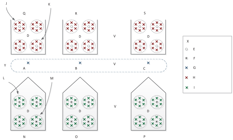
Partition the set of $y_{1}$-codewords $\Big\{\mathbf{y}_{1}(k,m_{11},i)\Big\}$ among the super-bins $\Big\{\mathcal{B}_{Y_{1}}(m_{10},m_{20})\Big\}$ according to the following rule. For each codeword $\mathbf{y}_{1}$ let $\mathcal{V}\big(\mathbf{y}_{1}\big)\subseteq\mathcal{C}_{V}$ be the set of all $v$-codewords in $\mathcal{C}_{V}$ that are jointly typical with $\mathbf{y}_{1}$. The super-bin that contains the codewords $\mathbf{y}_{1}$ is then randomly and uniformly drawn among the bins that are associated with the $v$-codewords in $\mathcal{V}\big(\mathbf{y}_{1}\big)$. If the set $\mathcal{V}\big(\mathbf{y}_{1}\big)$ is empty, an encoding error is declared. From symmetry considerations (when averaging over all codebooks), the bins $\Big\{\mathcal{B}_{Y_{1}}(m_{10},m_{20})\Big\}$ are approximately of equal sizes with a size differences that vanishes asymptotically as $n\to\infty$. Therefore, we henceforth ignore this subtlety and assume $\big|\mathcal{B}_{Y_{1}}(m_{10},m_{20})\big|=2^{n(R_{11}+R^{\prime}_{11})}$ for every $(m_{10},m_{20})\in\mathcal{M}_{10}\times\mathcal{M}_{20}$; accordingly, the $y_{1}$-codewords in the bin $\mathcal{B}_{Y_{1}}(m_{10},m_{20})$ are henceforth denoted by $\mathbf{y}_{1}(m_{10},m_{20},m_{11},i)$, where $m_{11}\in\mathcal{M}_{11}$ and $i\in\{1,\ldots,2^{nR^{\prime}_{11}}\}$. As such, each bin $\mathcal{B}_{Y_{1}}(m_{10},m_{20})$ constitutes a codebook for the private messages in $\mathcal{M}_{11}$, such that a $y_{1}$-bin, which contains $2^{nR^{\prime}_{11}}$ $y_{1}$-codewords, is associated with every private message $m_{11}\in\mathcal{M}_{11}$.

The structure of the codebook, while overlooking the binning of $\mathcal{C}_{V}$ for simplicity, is illustrated in Fig. 6.

Fig. 6: The codebook structure.

A-2 Encoding

To transmit the message pair $(m_{1},m_{2})=\big((m_{10},m_{11}),(m_{20},m_{22})\big)$, the encoder searches for a pair of indices $i\in\{1,\ldots,2^{nR^{\prime}_{11}}\}$ and $j\in\{1,\ldots,2^{nR^{\prime}_{22}}\}$ such that

$$\Big(\mathbf{v}(m_{10},m_{20}),\mathbf{u}(m_{10},m_{20},m_{22},j),\mathbf{y}_{1}(m_{10},m_{20},m_{11},i)\Big)\in\mathcal{T}_{\epsilon}^{(n)}(V,U,Y_{1})$$ (88)

where $\mathbf{u}(m_{10},m_{20},m_{22},j)\in\mathcal{C}_{U}(m_{10},m_{20})$ and $\mathbf{y}_{1}(m_{10},m_{20},m_{11},i)\in\mathcal{B}_{Y_{1}}(m_{10},m_{20})$. Upon finding such indices, a sequence $\mathbf{x}$ is randomly generated symbol-by-symbol according to the conditional PMF $P_{X|V,U,Y_{1}}$ and is transmitted through the channel.

A-3 Decoding Process

Denote the sequence received by Decoder $i$, $i\in\{1,2\}$, by $\mathbf{y}_{i}^{(r)}$.

Decoding at Decoder 1: Upon receiving $\mathbf{y}_{1}^{(r)}$, Decoder 1 searches for a unique triple $(\hat{m}_{10},\hat{m}_{20},\hat{m}_{11})\in\mathcal{M}_{10}\times\mathcal{M}_{20}\times\mathcal{M}_{11}$ such that there exists a index $\hat{i}\in\{1,\ldots,2^{nR^{\prime}_{11}}\}$ for which $\mathbf{y}_{1}(\hat{m}_{10},\hat{m}_{20},\hat{m}_{11},\hat{i})=\mathbf{y}_{1}^{(r)}$. If such a unique triple is found, then $\hat{m}_{1}\triangleq(\hat{m}_{10},\hat{m}_{11})$ is declared as the decoded message; otherwise, an error is declared.

Cooperation: Upon decoding $(\hat{m}_{10},\hat{m}_{20},\hat{m}_{11},\hat{i})$, Decoder 1 uses the cooperation links to convey the bin number of $\mathbf{v}(\hat{m}_{10},\hat{m}_{20})$ to Decoder 2. Namely, Decoder 1 shares with Decoder 2 the index $\hat{m}_{12}\in\mathcal{M}_{12}$ such that $\mathbf{v}(\hat{m}_{10},\hat{m}_{20})\in\mathcal{W}(\hat{m}_{12})$.

Decoding at Decoder 2: Having received $\hat{m}_{12}$ from Decoder 1 and $\mathbf{y}_{2}^{(r)}$ from the channel, Decoder 2 first searches for a unique pair $(\hat{\hat{m}}_{10},\hat{\hat{m}}_{20})\in\mathcal{M}_{10}\times\mathcal{M}_{20}$ such that $\mathbf{v}(\hat{\hat{m}}_{10},\hat{\hat{m}}_{20})\in\mathcal{W}(\hat{m}_{12})$ and

$$\Big(\mathbf{v}(\hat{\hat{m}}_{10},\hat{\hat{m}}_{20}),\mathbf{y}_{2}^{(r)}\Big)\in\mathcal{T}_{\epsilon}^{(n)}(V,Y_{2}).$$ (89)

If no such pair is found or the pair is not unique, an error is declared. Otherwise, upon decoding $(\hat{\hat{m}}_{10},\hat{\hat{m}}_{20})$, Decoder 2 searches for a unique $u$-bin $\hat{\hat{m}}_{22}\in\mathcal{M}_{22}$ such that there exists an index $\hat{\hat{j}}\in\{1,\ldots,2^{nR^{\prime}_{22}}\}$ for which

$$\Big(\mathbf{v}(\hat{\hat{m}}_{10},\hat{\hat{m}}_{20}),\mathbf{u}(\hat{\hat{m}}_{10},\hat{\hat{m}}_{20},\hat{\hat{m}}_{22},\hat{\hat{j}}),\mathbf{y}_{2}^{(r)}\Big)\in\mathcal{T}_{\epsilon}^{(n)}(V,U,Y_{2}).$$ (90)

If a unique $u$-bin is detected, Decoder 2 outputs $\hat{\hat{m}}_{2}\triangleq(\hat{\hat{m}}_{20},\hat{\hat{m}}_{22})$ as the decoded message; otherwise, an error is declared.

By standard error probability analysis (see Appendix B), we get that for the error probability to vanish as $n\to\infty$, the rate constraints in (7) must be satisfied. This shows that if $(R_{12},R_{1},R_{2})$ is inside the rate region specified in Theorem 1, then there exists a sequence of $(n,2^{nR_{12}},2^{nR_{1}},2^{nR_{2}})$ codes such that $P_{e}^{(n)}\rightarrow 0$ as $n\rightarrow\infty$, which completes the proof.

Appendix B Error Probability Analysis for the Achievability Proof of Theorem 1

Denote the transmitted messages by $(m_{1},m_{2})=\big((m_{10},m_{11}),(m_{20},m_{22})\big)$. The indices originally chosen by the encoder are denoted without accents (e.g., $m_{12}$ or $i$) while indices from the same alphabets that were not chosen by the encoder are denoted with a tilde (e.g., $\tilde{m}_{12}$ or $\tilde{i}$).

Encoding errors: An encoding error occurs if there exists a $y_{1}$-codeword that is not jointly typical with any of the codewords in $\mathcal{C}_{V}$. To account for this event, we take

$$R_{10}+R_{20}>I(V;Y_{1}).$$ (91)

With (91), the probability of the encoding error event vanishes as $n\to\infty$ by the covering lemma [44, Lemma 3.3]. But an encoding error also happens if there is no pair $(i,j)\in\{1,\ldots,2^{nR^{\prime}_{11}}\}\times\{1,\ldots,2^{nR^{\prime}_{22}}\}$ that satisfies (88), i.e., the $y_{1}$-bin and the $u$-bin that correspond to the messages $\big((m_{10},m_{11}),(m_{20},m_{22})\big)$ contain no jointly typical pair of codewords. By the Multivariate Covering Lemma [44, Lemma 8.2], the probability of this event also vanishes as $n\to\infty$ if we have

$$R^{\prime}_{11}+R^{\prime}_{22}>I(U;Y_{1}|V).$$ (92)

Decoder 1 errors: This happens only if there is more than one $y_{1}$-bin that contains the received $\mathbf{y}_{1}^{(r)}$. Suppose that the encoding was successful and (88) is satisfied. Accordingly, $\mathbf{y}_{1}^{(r)}\in\mathcal{T}_{\epsilon}^{(n)}(Y_{1})$ and therefore

$$P_{\mathbf{Y}_{1}}(\mathbf{y}_{1}^{(r)})\leq 2^{-n\big(H(Y_{1})-\delta(\epsilon)\big)}$$ (93)

where $\delta(\epsilon)\to 0$ when $\epsilon\to 0$. Hence, the probability that a specific $y_{1}$-codeword that was not chosen by the encoder (which by our code construction was generated independently of the received $\mathbf{y}_{1}^{(r)}$) happens to be the same as $\mathbf{y}_{1}^{(r)}$ is upper bounded by the RHS of (93). Furthermore, the total number of $y_{1}$-codewords outside the $y_{1}$-bin chosen by the encoder is $2^{nR^{\prime}_{11}}\cdot(2^{n(R_{10}+R_{20}+R_{11})}-1)$. By using the union bound, we obtain that the probability of a decoding error at Decoder 1 is at most

$$2^{n(R_{10}+R_{20}+R_{11}+R^{\prime}_{11})}\cdot 2^{-n\big(H(Y_{1})-\delta(\epsilon)\big)},$$ (94)

which tends to zero as $n\to\infty$ provided that

$$R_{10}+R_{20}+R_{11}+R^{\prime}_{11}=R_{1}+R_{20}+R^{\prime}_{11}<H(Y_{1})-\delta(\epsilon).$$ (95)

Cooperation decoding errors: An error occurs if either the codeword $\mathbf{v}(m_{10},m_{20})$ is not jointly typical with the $\mathbf{y}_{2}^{(r)}$ received at Decoder 2, or if a different $v$-codeword in the bin $\mathcal{W}(m_{12})$ happens to be jointly typical with $\mathbf{y}_{2}^{(r)}$. Assuming successful encoding, the probability of the former event tends to zero as $n\to\infty$ by (88) and by the Markov Lemma [44, Lemma 12.1]. To upper-bound the probability of the latter event, note that any $\mathbf{v}(\tilde{m}_{10},\tilde{m}_{20})$, where $(\tilde{m}_{10},\tilde{m}_{20})\neq(m_{10},m_{20})$, is independent of the transmitted $y_{1}$- and $u$-codewords and is, therefore, also independent of $\mathbf{y}_{2}^{(r)}$. By the Joint Typicality Lemma [44, Subsection 2.5] we have

$$\mathbb{P}\Big[(\mathbf{V}(\tilde{m}_{10},\tilde{m}_{20}),\mathbf{Y}_{2}^{(r)})\in\mathcal{T}_{2\epsilon}^{(n)}\Big]\leq 2^{-n\big(I(V;Y_{2})-\delta(\epsilon)\big)}$$ (96)

where the probability is computed with respect to a randomly chosen codebook. By using $\big|\mathcal{W}(m_{12})\big|=2^{n(R_{10}+R_{20}-R_{12})}$ and the union bound we get that the probability that there exists a codeword $\mathbf{v}(\tilde{m}_{10},\tilde{m}_{20})\in\mathcal{W}(m_{12})$, where $(\tilde{m}_{10},\tilde{m}_{20})\neq(m_{10},m_{20})$, that is jointly typical with $\mathbf{y}_{2}^{(r)}$ is at most

$$2^{n(R_{10}+R_{20}-R_{12})}\cdot 2^{-n\big(I(V;Y_{2})-\delta(\epsilon)\big)}.$$ (97)

(97) vanishes as $n\to\infty$ if

$$R_{10}+R_{20}-R_{12}<I(V;Y_{2})-\delta(\epsilon).$$ (98)

Decoder 2 errors: Assuming successful cooperation decoding, Decoder 2 has access to the correct $\mathbf{v}(m_{10},m_{20})$. Consequently, a decoding error at Decoder 2 occurs if either the codeword $\mathbf{u}(m_{10},m_{20},m_{22},j)$ is not jointly typical with $\big(\mathbf{v}(m_{10},m_{20}),\mathbf{y}_{2}^{(r)}\big)$, or if there exists a $u$-codeword in a different $u$-bin in the codebook $\mathcal{C}_{U}(m_{10},m_{20})$ that is jointly typical with $\big(\mathbf{v}(m_{10},m_{20}),\mathbf{y}_{2}^{(r)}\big)$. In a manner similar to that presented before, by assuming successful encoding and using the Markov Lemma [44, Lemma 12.1], we obtain that the probability of the former event tends to zero as $n\to\infty$. For the latter event, we again apply arguments analogous to those presented above and upper-bound its probability by

$$2^{n(R_{22}+R^{\prime}_{22})}\cdot 2^{-n\big(I(U;Y_{2}|V)-\delta(\epsilon)\big)}$$ (99)

which vanishes with $n$ provided

$$R_{22}+R^{\prime}_{22}<I(U;Y_{2}|V)-\delta(\epsilon).$$ (100)

Having (91), (92), (95), (98) and (100), we apply Fourier-Motzkin elimination (FME) while using (86), which yields that $P_{e}^{(n)}\to 0$ as the blocklength $n\to\infty$ if the following conditions are met:

$$R_{12} \geq I(V;Y_{1})-I(V;Y_{2})$$ (101a)

$$R_{1} \leq H(Y_{1})$$ (101b)

$$R_{2} \leq I(V,U;Y_{2})+R_{12}$$ (101c)

$$R_{1}+R_{2} \leq H(Y_{1}|V,U)+I(U;Y_{2}|V)+I(V;Y_{1}).$$ (101d)

Appendix C Proof of Theorem 2

C-A Achievability

The direct part of the proof is based on a coding scheme that achieves the corner points of the region in (8); the corner points are stated in (17)-(18) and illustrated in Fig 3. The scheme relies on WZ coding, binning and superposition coding.

Fix $\epsilon>0$ and a joint distribution $P_{X_{1},X_{2}}P_{V|X_{1}}P_{U|X_{2},V}P_{Y|X_{1},U,V}$ that has $P_{X_{2}}P_{Y|X_{2}}\mathds{1}_{\{X_{1}=f(Y)\}}$ as a marginal.

Codebook Generation: A codebook $\mathcal{C}_{V}$ that comprises $2^{nR_{v}}$ codewords $\mathbf{v}(i)$, where $i\in\{1,2,\ldots,2^{nR_{v}}\}$, is generated in an i.i.d. manner according to $P_{V}$. The codebook $\mathcal{C}_{V}$ is randomly partitioned into $2^{nR_{12}}$ bins indexed by $t_{12}\in\{1,2,\ldots,2^{nR_{12}}\}$ and denoted by $\mathcal{B}_{V}(t_{12})$. For every $\mathbf{v}\in\mathcal{C}_{V}$ a codebook $\mathcal{C}_{U}(\mathbf{v})$ is generated. Each codebook $\mathcal{C}_{U}(\mathbf{v})$ is assembled of $2^{nR_{u}}$ codewords $\mathbf{u}\big(\mathbf{v},j\big)$, $j\in\{1,2,\ldots,2^{nR_{u}}\}$, generated according to $\prod_{i=1}^{n}P_{U|V}\big(u_{i}(\mathbf{v},j)|v_{i}\big)$. Each $\mathcal{C}_{U}(\mathbf{v})$ codebook is randomly partitioned into $2^{nR_{2}^{\prime}}$ bins $\mathcal{B}_{U}(\mathbf{v},t_{2}^{\prime})$, where $t_{2}\in\{1,2,\ldots,2^{nR_{2}^{\prime}}\}$. Moreover, the set $\mathcal{T}_{\epsilon}^{(n)}(X_{1})$ is partitioned into $2^{R_{1}^{\prime}}$ bins $\mathcal{B}_{X_{1}}(t_{1}^{\prime})$, where $t_{1}^{\prime}\in\{1,2,\ldots,2^{nR_{1}^{\prime}}\}$.

To achieve (17), consider the following scheme:
Encoding at Encoder 1: Upon receiving $\mathbf{x}_{1}$, Encoder 1 searches a pair of indices $(i,t_{1}^{\prime})\in\{1,\ldots,2^{nR_{v}}\}\times\{1,\ldots,2^{nR_{1}^{\prime}}\}$ such that $\big(\mathbf{v}(i),\mathbf{x}_{1}\big)\in\mathcal{T}_{\epsilon}^{(n)}(V,X_{1})$ and $\mathbf{x}_{1}\in\mathcal{B}_{X_{1}}(t_{1}^{\prime})$. A concatenation $i$ and $t_{1}^{\prime}$ is conveyed to the decoder. The bin index of $\mathbf{v}(i)$, say $t_{12}$, is conveyed to Encoder 2 via the cooperation link. Having

$$R_{v}>I(V;X_{1})$$ (102)

ensures that such a codeword $\mathbf{v}(i)$ is found with high probability.

Decoding at Encoder 2: Upon receiving the input sequence $\mathbf{x}_{2}$ and the bin index $t_{12}$, Encoder 2 searches for an index $\hat{i}\in\{1,\ldots,2^{nR_{v}}\}$ such that $\mathbf{v}(\hat{i})\in\mathcal{B}_{V}(t_{12})$ and $\big(\mathbf{v}(\hat{i}),\mathbf{x}_{2}\big)\in\mathcal{T}_{\epsilon}^{(n)}(V,X_{2})$. Reliable decoding follows by having

$$R_{v}-R_{12}<I(V;X_{2}).$$ (103)

Encoding at Encoder 2: Upon decoding $\mathbf{v}(\hat{i})$, Encoder 2 searches for an index $j\in\{1,\ldots,2^{nR_{u}}\}$ such that $\mathbf{u}\big(\mathbf{v}(\hat{i}),j\big)\in\mathcal{C}_{U}(\mathbf{v}\big(\hat{i})\big)$ and $\Big(\mathbf{v}(\hat{i}),\mathbf{u}\big(\mathbf{v}(\hat{i}),j\big),\mathbf{x}_{2}\Big)\in\mathcal{T}_{\epsilon}^{(n)}(V,U,X_{2})$. The bin number of the chosen $\mathbf{u}\big(\mathbf{v}(\hat{i}),j\big)$, say $t_{2}^{\prime}$, is conveyed to the decoder. Choosing

$$R_{u}>I(U;X_{2}|V)$$ (104)

ensures that such a codeword $\mathbf{u}\big(\mathbf{v}(\hat{i}),j\big)$ is found.

Decoding and Output Generation: Upon receiving $(i,t_{1}^{\prime})$ from Encoder 1 and $t_{2}^{\prime}$ from Encoder 2, the decoder first identifies the codeword $\mathbf{v}(i)\in\mathcal{C}^{V}$ that is associated with the index $i$. Then it searches the bin $\mathcal{B}_{X_{1}}(t_{1}^{\prime})$ for a sequence $\hat{\mathbf{x}}_{1}$ such that $\big(\mathbf{v}(i),\hat{\mathbf{x}}_{1}\big)\in\mathcal{T}_{\epsilon}^{(n)}(V,X_{1})$. Reliable lossless reconstruction of $\mathbf{x}_{1}$ follows provided

$$R_{1}^{\prime}>H(X_{1}|V).$$ (105)

Having $\big(\mathbf{v}(i),\hat{\mathbf{x}}_{1}\big)$, the decoder searches for an index $\hat{j}\in\{1,\ldots,2^{nR_{u}}\}$ such that $\mathbf{u}\big(\mathbf{v}(i),\hat{j}\big)\in\mathcal{B}_{U}(t_{2}^{\prime})$ and $\Big(\mathbf{v}(i),\mathbf{u}\big(\mathbf{v}(i),\hat{j}\big),\hat{\mathbf{x}}_{1}\Big)\in\mathcal{T}_{\epsilon}^{(n)}(V,U,X_{1})$. To insure error-free decoding we take

$$R_{u}-R_{2}^{\prime}<I(U;X_{1}|V).$$ (106)

Finally, an output sequence $\mathbf{y}$ is generated according to $\prod_{k=1}^{n}P_{Y|X_{1},U,V}\Big(y_{k}\Big|\hat{x}_{1,k},u_{k}\big(\mathbf{v}(i),\hat{j}\big),v_{k}(i)\Big)$. By the choice of the joint distribution, this output sequence admits the desired coordination constraint.

By taking $(R_{1},R_{2})=(R_{1}^{\prime}+R_{v},R_{2}^{\prime})$ and applying the FME procedure on (102)-(106), we obtain the following rate bounds:

$$R_{12}>I(V;X_{1})-I(V;X_{2})=I(V;X_{1}|X_{2})$$ (107a)

$$R_{1}>H(X_{1}|V)+I(V;X_{1})=H(X_{1})$$ (107b)

$$R_{2}>I(U;X_{2}|V)-I(U;X_{1}|V)=I(U;X_{2}|X_{1},V).$$ (107c)

This implies that (17) is achievable.

To establish the achievability of (18) no binning of the codebooks $\mathcal{C}_{U}(\mathbf{v})$, where $\mathbf{v}\in\mathcal{C}_{V}$, is needed.

Encoding at Encoder 1: Upon receiving $\mathbf{x}_{1}$, Encoder 1 finds $\mathbf{v}(i)\in\mathcal{C}_{V}$ in a similar manner and conveys its bin index $t_{12}$ to Encoder 2. Moreover, it conveys the bin index of the received $\mathbf{x}_{1}$, say $t_{1}^{\prime}$, to the decoder. Again, by having (102), such a codeword $\mathbf{v}(i)$ is found with high probability.

Decoding at Encoder 2: Performed in a similar manner as before. Thus, (103) is required for reliable decoding.

Encoding at Encoder 2: Encoder 2 finds a codeword $\mathbf{u}\big(\mathbf{v}(\hat{i}),j\big)\in\mathcal{C}_{U}\big(\mathbf{v}(\hat{i})\big)$ in a manner similar to that presented in the previous scheme. Now, however, it sends to the decoder a concatenation of $\hat{i}$ and $j$. This decoding process requires (104).

Decoding and Output Generation: Upon receiving $t_{1}^{\prime}$ from Encoder 1 and $(\hat{i},j)$ from Encoder 2, the decoder first finds the $\mathbf{v}(\hat{i})\in\mathcal{C}_{V}$ that is associated with $\hat{i}$ and the $\mathbf{u}\big(\mathbf{v}(\hat{i},j)\big)\in\mathcal{C}_{U}\big(\mathbf{v}(\hat{i})\big)$ that is associated with $\big(\mathbf{v}(\hat{i}),j\big)$. Having $\Big(\mathbf{v}(\hat{i}),\mathbf{u}\big(\mathbf{v}(\hat{i}),j\big)\Big)$, it searches the bin $\mathcal{B}_{X_{1}}(t_{1}^{\prime})$ for a sequence $\hat{\mathbf{x}}_{1}$ such that $\Big(\mathbf{v}(\hat{i}),\mathbf{u}\big(\mathbf{v}(\hat{i}),j\big),\hat{\mathbf{x}}_{1}\Big)\in\mathcal{T}_{\epsilon}^{(n)}(V,U,X_{1})$. Reliable lossless reconstruction of $\mathbf{x}_{1}$ is ensured provided

$$R_{1}^{\prime}>H(X_{1}|V,U).$$ (108)

Finally, an output sequence $\mathbf{y}$ is generated in a manner similar to this presented before.

Taking $(R_{1},R_{2})=(R_{1}^{\prime},R_{v}+R_{u})$ and applying FME on (102)-(104), and (108) yields the following bounds:

$$R_{12}>I(V;X_{1})-I(V;X_{2})=I(V;X_{1}|X_{2})$$ (109a)

$$R_{1}>H(X_{1}|V,U)$$ (109b)

$$R_{2}>I(V;X_{1})+I(U;X_{2}|V).$$ (109c)

Thus (18) is also achievable, which concludes the proof of achievability.

C-B Converse

Due to the structure of the joint distribution stated in Theorem 2, we rewrite the mutual information measure in (8) as

$$R_{2} \geq I(U;X_{2}|X_{1},V)\stackrel{{\scriptstyle(a)}}{{=}}I(V;X_{2}|X_{1})+I(U;X_{2}|X_{1},V)=I(V,U;X_{2}|X_{1}).$$ (110)

where (a) follows from the Markov relation $V-X_{1}-X_{2}$.

By Fano’s inequality we have

$$H(X_{1}^{n}|T_{1},T_{2})\leq n\epsilon_{n},.$$ (111)

For the lower bound on $R_{12}$, consider

$$nR_{12} \geq H(T_{12})$$

$$\stackrel{{\scriptstyle(a)}}{{=}}I(T_{12};X_{1}^{n},X_{2}^{n})$$

$$=\sum_{i=1}^{n}I(T_{12};X_{1}^{n},X_{2,i}|X_{2,i+1}^{n})$$

$$\geq\sum_{i=1}^{n}I(T_{12};X_{1,i},X_{2,i}|X_{1}^{n\backslash i},X_{2,i+1}^{n})$$

$$\stackrel{{\scriptstyle(b)}}{{=}}\sum_{i=1}^{n}I(T_{12},X_{1}^{n\backslash i},X_{2,i+1}^{n};X_{1,i},X_{2,i})$$

$$\geq\sum_{i=1}^{n}I(T_{12},X_{1}^{n\backslash i},X_{2,i+1}^{n};X_{1,i}|X_{2,i})$$

$$\stackrel{{\scriptstyle(c)}}{{=}}\sum_{i=1}^{n}I(V_{i};X_{1,i}|X_{2,i})$$ (112)

where:
(a) follows because $T_{12}$ is a deterministic function of $X_{1}^{n}$;
(b) follows because the sequences $\big\{(X_{1,i},X_{2,i})\big\}_{i=1}^{n}$ are drawn in an i.i.d. manner;
(c) follows by defining $V_{i}\triangleq(T_{12},X_{1}^{n\backslash i},X_{2,i+1}^{n})$.

Next, for $R_{1}$ we have

$$nR_{1} \geq H(T_{1})$$

$$\geq H(T_{1}|T_{2})$$ (113)

$$\stackrel{{\scriptstyle(a)}}{{=}}I(T_{1};X_{1}^{n}|T_{2})$$

$$=H(X_{1}^{n}|T_{2})-H(X_{1}^{n}|T_{1},T_{2})$$

$$\stackrel{{\scriptstyle(b)}}{{\geq}}\sum_{i=1}^{n}H(X_{1,i}|T_{2},X_{1}^{i-1})-n\epsilon_{n}$$ (114)

$$\geq\sum_{i=1}^{n}H(X_{1,i}|T_{2},T_{12},X_{1}^{n\backslash i},X_{2,i+1}^{n})-n\epsilon_{n}$$

$$\stackrel{{\scriptstyle(c)}}{{=}}\sum_{i=1}^{n}H(X_{1,i}|V_{i},U_{i})-n\epsilon_{n}$$ (115)

where:
(a) follows because $T_{1}$ is a deterministic function of $X_{1}^{n}$;
(b) follows from (111) and the mutual information chain rule;
(c) follows by defining $U_{i}\triangleq T_{2}$ and from the definition of $V_{i}$.

The rate bound on $R_{2}$ follows from

$$nR_{2} \geq H(T_{2})$$

$$\geq H(T_{2}|X_{1}^{n})$$

$$\geq I(T_{2};X_{2}^{n}|X_{1}^{n})$$

$$=\sum_{i=1}^{n}I(T_{2};X_{2,i}|X_{1}^{n\backslash i},X_{2,i+1}^{n},X_{1,i})$$

$$\stackrel{{\scriptstyle(a)}}{{=}}\sum_{i=1}^{n}I(T_{2},X_{1}^{n\backslash i},X_{2,i+1}^{n};X_{2,i}|X_{1,i})$$

$$\stackrel{{\scriptstyle(b)}}{{=}}\sum_{i=1}^{n}I(T_{2},T_{12},X_{1}^{n\backslash i},X_{2,i+1}^{n};X_{2,i}|X_{1,i})$$

$$\stackrel{{\scriptstyle(c)}}{{=}}\sum_{i=1}^{n}I(V_{i},U_{i};X_{2,i}|X_{1,i})$$ (116)

where:
(a) follows because the sequences $\big\{(X_{1,i},X_{2,i})\big\}_{i=1}^{n}$ are drawn in an i.i.d. manner;
(b) follows because $T_{12}$ is a deterministic function of $X_{1}^{n}$;
(c) follows because conditioning reduces entropy and from the definition of $(U_{i},V_{i})$.

Finally for the sum of rates, we first have

$$n(R_{1}+R_{2})\geq H(T_{1},T_{2})=H(T_{2})+H(T_{1}|T_{2}).$$ (117)

For the first term in (117) we have

$$H(T_{2}) \geq I(T_{2};X_{1}^{n},X_{2}^{n})$$

$$=\sum_{i=1}^{n}I(T_{2};X_{1}^{n},X_{2,i}|X_{2,i+1}^{n})$$

$$\geq\sum_{i=1}^{n}I(T_{2};X_{1,i},X_{2,i}|X_{1}^{n\backslash i},X_{2,i+1}^{n})$$

$$\stackrel{{\scriptstyle(a)}}{{=}}\sum_{i=1}^{n}I(T_{2},X_{1}^{n\backslash i},X_{2,i+1}^{n};X_{1,i},X_{2,i})$$

$$=\sum_{i=1}^{n}\big[I(T_{2},T_{12},X_{1}^{n\backslash i},X_{2,i+1}^{n};X_{1,i},X_{2,i})-I(T_{12};X_{1,i},X_{2,i}|T_{2},X_{1}^{n\backslash i},X_{2,i+1}^{n})\big]$$

$$\stackrel{{\scriptstyle(b)}}{{=}}\sum_{i=1}^{n}\big[I(V_{i},U_{i};X_{1,i},X_{2,i})-H(X_{1,i},X_{2,i}|T_{2},X_{1}^{n\backslash i},X_{2,i+1}^{n})+H(X_{1,i},X_{2,i}|T_{2},T_{12},X_{1}^{n\backslash i},X_{2,i+1}^{n})\big]$$

$$\stackrel{{\scriptstyle(c)}}{{=}}\sum_{i=1}^{n}\big[I(V_{i},U_{i};X_{1,i},X_{2,i})+H(X_{1,i}|V_{i},U_{i})-H(X_{1,i},X_{2,i}|T_{2},X_{1}^{n\backslash i},X_{2,i+1}^{n})$$

$$\ \ \ \ \ \ \ \ \ \ \ \ \ \ \ \ \ \ \ \ \ \ \ \ \ \ \ \ \ \ \ \ \ \ \ \ \ \ \ \ \ \ \ \ \ \ \ \ \ \ \ \ \ \ \ \ \ \ \ \ \ \ \ \ \ \ \ \ \ \ \ \ \ \ \ +H(X_{2,i}|T_{2},T_{12},X_{1}^{n\backslash i},X_{2,i+1}^{n},X_{1,i})\big]$$

$$\stackrel{{\scriptstyle(d)}}{{=}}\sum_{i=1}^{n}\big[I(V_{i},U_{i};X_{1,i},X_{2,i})+H(X_{1,i}|V_{i},U_{i})-H(X_{1,i}|T_{2},X_{1}^{n\backslash i},X_{2,i+1}^{n})$$

$$\ \ \ \ \ \ \ \ \ \ \ \ \ \ \ \ \ \ \ \ \ \ \ \ \ \ \ \ \ -H(X_{2,i}|T_{2},T_{12},X_{1}^{n\backslash i},X_{2,i+1}^{n},X_{1,i})+H(X_{2,i}|T_{2},T_{12},X_{1}^{n\backslash i},X_{2,i+1}^{n},X_{1,i})\big]$$

$$\stackrel{{\scriptstyle(e)}}{{=}}\sum_{i=1}^{n}\big[I(V_{i},U_{i};X_{1,i},X_{2,i})+H(X_{1,i}|V_{i},U_{i})-\Delta_{i}\big]$$ (118)

where:
(a) follows because $\big\{(X_{1,i},X_{2,i})\big\}_{i=1}^{n}$ are drawn in an i.i.d. manner;
(b) and (c) follow from the definition of $(U_{i},V_{i})$;
(d) follows because $T_{12}$ is a deterministic function of $X_{1}^{n}$;
(e) follows by defining

$$\Delta_{i}\triangleq H(X_{1,i}|T_{2},X_{1}^{n\backslash i},X_{2,i+1}^{n}),$$ (119)

The second term in (117) is lower bounded by

$$H(T_{1}|T_{2}) \stackrel{{\scriptstyle(a)}}{{\geq}}\sum_{i=1}^{n}H(X_{1,i}|T_{2},X_{1}^{i-1})-n\epsilon_{n}$$

$$\geq\sum_{i=1}^{n}H(X_{1,i}|T_{2},X_{1}^{n\backslash i},X_{2,i+1}^{n})-\epsilon_{n}$$

$$\stackrel{{\scriptstyle(b)}}{{=}}\sum_{i=1}^{n}\Delta_{i}$$ (120)

where (a) follows by repeating the same steps (113)-(114) in the lower bounding of $R_{1}$, while (b) follows from (119).
By substituting (118) and (120) into (117) we have

$$n(R_{1}+R_{2})\geq\sum_{i=1}^{n}\Big[I(V_{i},U_{i};X_{1,i},X_{2,i})+H(X_{1,i}|V_{i},U_{i})\Big]-n\epsilon_{n}.$$ (121)

The upper bounds in (112), (115), (116) and (121) are rewritten by introducing a time sharing random variable $Q$ that is uniformly distributed over the set $\{1,2,...,n\}$. The rate bound on $R_{12}$ is rewritten as

$$nR_{12} \geq n\sum_{i=1}^{n}\mathbb{P}[Q=i]I(V_{Q};X_{1,Q}|X_{2,Q},Q=i)$$ (122)

$$=nI(V_{Q};X_{1,Q}|X_{2,Q},Q)$$ (123)

$$\stackrel{{\scriptstyle(a)}}{{=}}nI(V_{Q},Q;X_{1,Q}|X_{2,Q})$$ (124)

where (a) follows because $Q$ is independent of the pair $(X_{1,Q},X_{2,Q})$ (see property 1 in [31, Section IIV, Subsection B]). By rewriting (115), (116) and (121) in the same manner the region obtained is convex. This follows from the presence of the time sharing random variable $Q$ in all the mutual information and entropy terms.

Next, let $V\triangleq(V_{Q},Q)$, $U\triangleq U_{Q}$. By using the time-mixing properties (property 2 in [31, Section IIV, Subsection B]), we have

$$R_{12} \geq I(V;X_{1}|X_{2})$$ (125)

$$R_{1} \geq H(X_{1}|V,U)$$ (126)

$$R_{2} \geq I(U;X_{2}|X_{1},V)$$ (127)

$$R_{1}+R_{2} \geq H(X_{1}|V,U)+I(V,U;X_{1},X_{2}).$$ (128)

To complete the converse remains to show that the following Markov relations hold:

$$V-X_{1}-X_{2}$$ (129)

$$U-(X_{2},V)-X_{1}$$ (130)

$$Y-(X_{1},U,V)-X_{2}.$$ (131)

We prove that the Markov relations in (129)-(131) hold for every $i\in\{1,\ldots,n\}$; upon doing so, deriving that the relations still hold in their single letter (as stated in (129)-(131)) is straightforward.

For (129), recall that $V_{i}=(T_{12},X_{1}^{n\backslash i},X_{2,i+1}^{n})$, and consider

$$0 \leq I(T_{12},X_{1}^{n\backslash i},X_{2,i+1}^{n};X_{2,i}|X_{1,i})$$

$$\stackrel{{\scriptstyle(a)}}{{=}}I(X_{1}^{n\backslash i},X_{2,i+1}^{n};X_{2,i}|X_{1,i})\stackrel{{\scriptstyle(b)}}{{=}}0$$

where (a) follows because $T_{12}$ is a deterministic function of $X_{1}^{n}$, while (b) follows because the sequences $\{(X_{1,i},X_{2,i})\}_{i=1}^{n}$ are drawn in an i.i.d. manner. Thus (129) holds.

To establish (130), we use Lemma 1 in [45]. Since $U_{i}=T_{2}$ we have

$$0 \leq I(T_{2};X_{1,i}|X_{2,i},T_{12},X_{1}^{n\backslash i},X_{2,i+1}^{n})$$

$$\leq I(T_{2};X_{1,i},X_{1,i+1}^{n}|X_{2,i},T_{12},X_{1}^{i-1},X_{2,i+1}^{n}).$$ (132)

Set

$$A_{1}=X_{1}^{i-1}\ ,\ \ \ A_{2}=(X_{1,i},X_{1,i+1}^{n}),$$

$$B_{1}=X_{2}^{i-1}\ ,\ \ \ B_{2}=(X_{2,i},X_{2,i+1}^{n}).$$

Thus, (132) is rewritten as

$$0 \leq I(T_{2};A_{2}|T_{12},A_{1},B_{2}).$$ (133)

By noting that $T_{12}=T_{12}(A_{1},A_{2})$, $T_{2}=(T_{12},B_{1},B_{2})$ and $P_{A_{1},A_{2},B_{1},B_{2}}=P_{A_{1},B_{1}}P_{A_{2},B_{2}}$ and applying the result of [45, Lemma 1, Conclusion 2] we have

$$0\leq I(T_{2};A_{2}|T_{12},A_{1},B_{2})=0.$$ (134)

This, in turn, implies (130).

Finally, to prove (131), recall that $Y^{n}$ (and, in particular, $Y_{i}$) is a deterministic function of $(T_{1},T_{2})$. Rewriting (131) explicitly, we have

$$Y_{i}-(T_{2},T_{12},X_{1}^{n},X_{2,i+1}^{n})-X_{2,i}.$$ (135)

Since $T_{1}$ is defined by $X_{1}^{n}$ it can be added to the middle link of the Markov chain in (135), which establishes the desired Markov property. This concludes the converse.

Appendix D Derivation of the Region in (60) from (59)

Denote the regions characterized by (59) and (60) by $\mathcal{C}_{RBC}$ and $\mathcal{R}$, respectively. Note that $\mathcal{R}$ is achievable from $\mathcal{C}_{RBC}$ by taking $X_{1}$ to be independent of $(V,U,X)$ and applying a coding scheme in which the transmission rate via the relay channel is $R_{12}$. Thus $\mathcal{R}\subseteq\mathcal{C}_{RBC}$.

Next, we show that $\mathcal{C}_{RBC}\subseteq\mathcal{R}$. Recall that the proof of Theorem 8 in [12] relies on Theorem 4 in that same work, which characterized an upper bound on the capacity region of a general RBC. In the proof of Theorem 4 (see [12, Appendix II]), the auxiliary random variables $V_{i}$ and $U_{i}$ are defined as

$$V_{i}=(M_{0},Y_{1}^{i-1},Y_{2,i+1}^{n})\ \ ;\ \ V_{i}=(M_{2},Y_{1}^{i-1},Y_{2,i+1}^{n}).$$ (136)

$M_{0}$ is a common message that was also considered in that work. Since $X_{1,i}$ is a deterministic function of $Y_{1}^{i-1}$, $X_{1,i}$ is also a deterministic function of $V_{i}$ (or $U_{i}$). Furthermore, since this relation holds for every $i\in\{1,\ldots,n\}$ it holds for the single-letter form. In particular, we find that $X_{1}$ is a deterministic function of $V$. The information measures defining the rate bounds in $\mathcal{R}_{1}$ can then be upper bounded as follows. For $R_{1}$ we have

$$R_{1}\leq H(Y_{1}|X_{1})\leq H(Y_{1}).$$ (137)

For the rate bound on $R_{2}$ consider

$$R_{2} \leq I(V,U,X_{1};Y_{21})+H(Y_{22}|Y_{21})$$

$$\stackrel{{\scriptstyle(a)}}{{\leq}}I(V,U;Y_{21})+H(Y_{22})$$

$$\stackrel{{\scriptstyle(b)}}{{\leq}}I(V,U;Y_{21})+R_{12}$$ (138)

where (a) follows because $X_{1}$ is a deterministic function of $V$ and since conditioning reduces entropy, while (b) follows because the relay channel is deterministic with capacity $R_{12}$.

Next, for the first bound on the sum of rates, we have

$$R_{1}+R_{2} \leq H(Y_{1}|V,U,X_{1})+I(U;Y_{21}|V,X_{1})+I(V;Y_{1}|X_{1})$$

$$\stackrel{{\scriptstyle(a)}}{{\leq}}H(Y_{1}|V,U)+I(U;Y_{21}|V)+I(V;Y_{1}).$$ (139)

Here (a) follows from the same reason as in the derivation of (138).

Finally, the second bound on $R_{1}+R_{2}$ is upper bounded as

$$R_{1}+R_{2} \leq H(Y_{1}|V,U,X_{1})+I(V,U,X_{1};Y_{21})+H(Y_{22}|Y_{21})$$

$$\stackrel{{\scriptstyle(a)}}{{\leq}}H(Y_{1}|V,U)+I(V,U;Y_{21})+H(Y_{22})$$

$$\stackrel{{\scriptstyle(b)}}{{\leq}}H(Y_{1}|V,U)+I(V,U;Y_{21})+R_{12}.$$ (140)

Once again, the reasoning for (a) and (b) is similar to that presented in the derivation of (138).

To complete the proof, it remains to show that taking the union only over joint distributions in which $X_{1}$ is independent of $(V,U,X)$ exhausts the entire region. Indeed, since the rate bounds in (137)-(140) do not involve $X_{1}$ nor $Y_{22}$, the region does not change if the union is only over joint distribution with the desired independence property. Thus $\mathcal{C}_{RBC}\subseteq\mathcal{R}$, which completes the proof.

Appendix E Equivalence Between the Regions in (7) and (59)

The capacity region of the semi-deterministic BC with cooperation stated in Theorem 1 is denoted by $\mathcal{C}$. Furthermore, the capacity region of the reduces RBC characterized by (60) is denoted by $\mathcal{C}_{RBC}$.

For the inclusion $\mathcal{C}\subseteq\mathcal{C}_{RBC}$, let $(R_{12},R_{1},R_{2})\in\mathcal{C}$ be a rate triple achieved by $(V,U,X)$. By taking $V^{\star}=V$ and $U^{\star}=U$, it follows that the same rate triple $(R_{12},R_{1},R_{2})$ in also contained in $\mathcal{C}_{RBC}$, as it is achieved by $(V^{\star},U^{\star},X)$ (namely, substituting (7a) into (7d) yields (60d)).

Next, we establish that $\mathcal{C}_{RBC}\subseteq\mathcal{C}$. Let $(R_{12},R_{1},R_{2})\in\mathcal{C}_{RBC}$ be a rate triple achieved by $(V,U,X)$. Further assume that

$$R_{12}<I(V;Y_{1})-I(V;Y_{2})$$ (141)

(otherwise, all four inequalities in (7) clearly hold). Accordingly, there is a real number $\gamma>0$ such that

$$R_{12}=I(V;Y_{1})-I(V;Y_{2})-\gamma.$$ (142)

The definition of $V^{\star}$ follows similar lines to these presented in Section V. Define $V^{\star}\triangleq(\Theta,\widetilde{V})$, where $\Theta\sim\mbox{Ber}\left(\lambda\right)$, $\lambda\in[0,1]$, is a binary random variable independent of $(V,U,X)$ that takes values in $\mathcal{O}=\{\theta_{1},\theta_{2}\}$, and

$$\widetilde{V}=\begin{cases}V\ ,&\Theta=\theta_{1}\\ \emptyset\ ,&\Theta=\theta_{2}\end{cases}.$$ (143)

Furthermore, let

$$\lambda=\frac{I(V;Y_{1})-I(V;Y_{2})-\gamma}{I(V;Y_{1})-I(V;Y_{2})}$$ (144)

and define $U^{\star}=(V,U)$.

With respect to this choice of $(V^{\star},U^{\star})$, consider

$$I(V^{\star};Y_{1})-I(V^{\star};Y_{2}) =\lambda\Big[I(V;Y_{1})-I(V;Y_{2})\Big]\stackrel{{\scriptstyle(a)}}{{=}}I(V;Y_{1})-I(V;Y_{2})-\gamma\stackrel{{\scriptstyle(b)}}{{=}}R_{12}$$ (145)

where (a) follows form the choice of $\lambda$ in (144) and (b) follows from (142). Thus, (7a) is satisfied.

Next, by the definition of $U^{\star}$ and because (7b)-(7c) are valid we obtain (60a)-(60b). Thus, it remains to show that (7d) holds. Consider the following chain of steps:

$$H(Y_{1}|V^{\star},U^{\star})+I(U^{\star};Y_{2}|V^{\star})+I(V^{\star};Y_{1}) =H(Y_{1}|V^{\star},U^{\star})+I(V^{\star},U^{\star};Y_{2})+I(V^{\star};Y_{1})-I(V^{\star};Y_{2})$$

$$\stackrel{{\scriptstyle(a)}}{{=}}H(Y_{1}|V,U)+I(V,U;Y_{2})+R_{12}\stackrel{{\scriptstyle(b)}}{{\geq}}R_{1}+R_{2}$$ (146)

where (a) follows from the definition of $U^{\star}$ and (145), while (b) follows from (60d). This implies that (7d) is also satisfied and yields the desired inclusion, that is, $\mathcal{C}_{RBC}\subseteq\mathcal{C}$. This concludes the proof.

Appendix F Derivation of the Region in (62)

We show that the optimal rate region for the SW problem with one-sided encoder cooperation is given by (62) and that this region is obtained from the coordination capacity region of the AK problem with cooperation stated in Theorem 1. To prove achievability, we substitute $U=X_{2}$ into the rate bounds in (8) and obtain

$$R_{12} \geq I(V;X_{1}|X_{2})$$

$$R_{1} \geq H(X_{1}|X_{2})-I(V;X_{1}|X_{2})$$

$$R_{2} \geq H(X_{2}|X_{1})$$

$$R_{1}+R_{2} \geq H(X_{1},X_{2}).$$ (147)

Note that the structure of the region in (62) implies $R_{12}\leq H(X_{1}|X_{2})$. Thus, it suffices to show that for $0\leq R_{12}\leq H(X_{1}|X_{2})$ there is a random variable $V$ that admits the Markov property $V-X_{1}-X_{2}$ such that $I(V;X_{1}|X_{2})=R_{12}$. Since $R_{12}\leq H(X_{1}|X_{2})$, there is a real number $\gamma\geq 0$ such that

$$R_{12}=H(X_{1}|X_{2})-\gamma.$$ (148)

Define the auxiliary random variable $V$ as follows. Let $\Theta\sim\mbox{Ber}\left(\lambda\right)$, $\lambda\in[0,1]$, be a binary random variable independent of $(X_{1},X_{2})$ that takes values in $\mathcal{O}=\{\theta_{1},\theta_{2}\}$, and let

$$\widetilde{V}=\begin{cases}X_{1}\ ,&\Theta=\theta_{1}\\ \emptyset\ ,&\Theta=\theta_{2}\end{cases}.$$ (149)

We define $V\triangleq(\Theta,\widetilde{V})$ while taking

$$\lambda=\frac{H(X_{1}|X_{2})-\gamma}{H(X_{1}|X_{2})}.$$ (150)

By (149) and (150) we have

$$I(V;X_{1}|X_{2}) =\lambda I(X_{1};X_{1}|X_{2})+\bar{\lambda}I(\emptyset;X_{1}|X_{2})$$

$$=\lambda H(X_{1}|X_{2})+\bar{\lambda}\cdot 0$$

$$=H(X_{1}|X_{2})-\gamma=R_{12}.$$

This establishes that (62) is achievable.

To prove the optimality of (62) we have the following converse. For the lower bound on $R_{1}$ we have

$$nR_{1} \geq H(T_{1})$$

$$=H(T_{1},T_{12})-H(T_{12}|T_{1})$$

$$\stackrel{{\scriptstyle(a)}}{{\geq}}H(T_{1},T_{12}|X_{2}^{n})-H(T_{12})$$

$$\stackrel{{\scriptstyle(b)}}{{\geq}}I(T_{1},T_{12};X_{1}^{n}|X_{2}^{n})-nR_{12}$$

$$\stackrel{{\scriptstyle(c)}}{{=}}H(X_{1}^{n}|X_{2}^{n})-H(X_{1}^{n}|T_{1},T_{12},X_{2}^{n},T_{2})-nR_{12}$$

$$\stackrel{{\scriptstyle(d)}}{{\geq}}H(X_{1}^{n}|X_{2}^{n})-nR_{12}-n\epsilon_{n}$$

$$\stackrel{{\scriptstyle(e)}}{{=}}\sum_{i=1}^{n}H(X_{1,i}|X_{2,i})-nR_{12}-n\epsilon_{n}$$

where:
(a) follows because conditioning reduces entropy;
(b) follows because $|\mathcal{T}_{12}|=2^{nR_{12}}$;
(c) follows because $T_{2}$ is a deterministic function of $(T_{12},X_{2}^{n})$;
(d) follows by Fano’s inequality according to which $H(X_{1}^{n}|T_{1},T_{2})\leq\epsilon_{n}$, where $\lim_{n\to\infty}\epsilon_{n}=0$.
(e) follows because the sequences $\big\{(X_{1,i},X_{2,i})\big\}_{i=1}^{n}$ are drawn in an i.i.d. manner.

The lower bounds on $R_{2}$ and $R_{1}+R_{2}$ are established as for the case without cooperation. This characterizes (62) as the optimal rate region for the SW problem with one-sided encoder cooperation.

References

- [1] F. M. J. Willems. The discrete memoryless multiple access channel with partially cooperating encoders. IEEE Trans. Inf. Theory, 29(6):441–445, May 1983.
- [2] S. I. Bross, A. Lapidoth, and M. A. Wigger. The Gaussian MAC with conferencing encoders. In Proc. Int. Symp. Inf. Theory, pages 2702–2706, Toronto, Canada, Jul. 2008.
- [3] O. Simeone, D. Gündüz, H. V. Poor, A. J. Goldsmith, and S. Shamai (Shitz). Compound multiple-access channels with partial cooperation. IEEE Trans. Inf. Theory, 55(6):2425–2441, Jun 2009.
- [4] M.Wiese, H. Boche, I. Bjelakovic, and V. Jungnickel. The compound multiple access channel with partially cooperating encoders. IEEE Trans. Inf. Theory, 57(5):30453066, May 2011.
- [5] R. Dabora and S. D. Servetto. Broadcast channels with cooperating decoders. IEEE Trans. Inf. Theory, 52:5438–5454, 2006.
- [6] Y. Liang and V. V. Veeravalli. Cooperative relay broadcast channels. IEEE Trans. Inf. Theory, 51(3):900–928, Mar 2007.
- [7] S. I. Gelfand and M. S. Pinsker. Capacity of a broadcast channel with one deterministic component. Problemy Peredachi Informatsii (Problems of Inform. Transm.), 16(1):17–25, Jan-Mar 1980.
- [8] K. Marton. A coding theorem for the discrete memoryless broadcast channel. IEEE Trans. Inf. Theory, 25(3):306–311, May 1979.
- [9] A. Lapidoth and L. Wang. The state-dependent semideterministic broadcast channel. IEEE Trans. Inf. Theory, 59(4):2242–2251, Apr. 2013.
- [10] S. I. Gelfand and M. S. Pinsker. Coding for channel with random parameters. Problems of Control Theory, 9:19–31, 1980.
- [11] T. A. Courtade and T. Weissman. Multiterminal source coding under logarithmic loss. IEEE Trans. Inf. Theory, 60(1):740–761, Jan. 2014.
- [12] Y. Liang and G. Kramer. Rate regions for relay broadcast channels. IEEE Trans. Inf. Theory, 53(10):3517–3535, Oct 2007.
- [13] H. Asnani, H. H. Permuter, and T. Weissman. Successive refinement with decoder cooperation and its channel coding duals. IEEE Trans. Inf. Theory, 59(9):5511–5533, Sep 2013.
- [14] C. E. Shannon. Coding theorems for a discrete source with a fidelity criterion. IRE Nat. Conv. Rec., pages 142–163, 1959.
- [15] T. M. Cover and M. Chiang. Unified duality between channel capacity and rate distortion with state information. IEEE Trans. Inf. Theory, 48(6):1629–1638, Jun. 2002.
- [16] S. S. Pradhan, J. Chou, and K. Ramchandran. Duality between source coding and channel coding and its extension to the side information case. IEEE Trans. Inf. Theory, 49(5):1181–1203, May 2003.
- [17] A. Gupta and S. Verdú. Operational duality between lossy compression and channel coding. IEEE Trans. Inf. Theory, 57(6):3171–3179, Jun 2011.
- [18] W. Yu. Duality and the value of cooperation in distributed source and channel coding problems. In Proc. 41st Annu. Allerton Conf. Commun., Control and Comput., Monticell, Illinois, United States, 2003.
- [19] H. Wang and P. Viswanath. Fixed binning schemes: An operational duality between channel and source coding problems with side information. In in Proc. Int. Symp. Inf. Theory, Chicago, Illinois, United States, Jun. 2004.
- [20] L. Dikstein, H. H. Permuter, and S. Shamai (Shitz). MAC with action-dependent state information at one encoder. Submitted for publication to IEEE Trans. Inf. Theory, 2012. http://arxiv.org/abs/1212.4626.
- [21] T. Berger. Multiterminal source coding. In G. Longo, editor, Information Theory Approach to Communications, volume 229, pages 171–231. CISM Cource and Lecture, 1978.
- [22] S. Y. Tung. Multiterminal source coding. PhD thesis, Cornell University, New York, United States, May 1978.
- [23] D. Slepian and J. Wolf. Noiseless coding of correlated information sources. IEEE Trans. Inf. Theory, 19(4):471–480, Jul. 1973.
- [24] A. D. Wyner and J. Ziv. The rate-distortion function for source coding with side information at the decoder. IEEE Trans. Inf. Theory, 22(1):1–10, Jan. 1976.
- [25] A. B. Wagner, S. Tavildar, and P. Viswanath. Rate region of the quadratic gaussian two-encoder source-coding problem. IEEE Trans. Inf. Theory, 54(5):1938–1961, May 2008.
- [26] R. Ahlswede and J. Korner. Source coding with side information and a converse for degraded broadcast channels. IEEE Trans. Inf. Theory, 21(6):629–637, 1975.
- [27] A. D. Wyner. The common information of two dependent random variables. IEEE Trans. Inf. Theory, 21(2):163–179, Mar. 1975.
- [28] G. Kramer and S. A. Savari. Data compression with commuting density operators. In IEEE Int. Symp. Inf. Theory, page 115, Lausanne, Switzerland, Jun.-Jul. 2002.
- [29] G. Kramer and S. A. Savari. Communicating probability distributions. IEEE Trans. Inf. Theory, 53(2):518–525, Feb. 2007.
- [30] V. Anantharam and V. Borkar. Common randomness and distributed control; A counterexample. Syst. Control Lett., 56:568–572, 2007.
- [31] P. W. Cuff, H. H. Permuter, and T. M. Cover. Coordination capacity. IEEE Trans. Inf. Theory, 56(9):4181–4206, Sep. 2010.
- [32] A. Bereyhi, M. Bahrami, M. Mirmohseni, and M. R. Aref. Empirical coordination in a triangular multiterminal network. In In. Proc. Symp. Inf. theory, Istanbul, Turkey, Jul. 2013.
- [33] T. M. Cover. A proof of the data compression theorem of Slepian and Wolf for ergodic sources. IEEE Trans. Inf. Theory, 22(2):226–228, Mar. 1975.
- [34] T. M. Cover. Broadcast channels. IEEE Trans. Inf. Theory, 18(1):2–14, Jan. 1972.
- [35] T. Berger and R.W. Yeung . Multiterminal source encoding with one distortion criterion. IEEE Trans. Inf. Theory, 35(2):228–236, Mar. 1989.
- [36] A. B. Wagner, B. G. Kelly, and Y. Altuğ. Distributed rate-distortion with common components. IEEE Trans. Inf. Theory, 57(7):4035–4057, Jul. 2011.
- [37] Csiszár and Korner. Information Theory: Coding Theorems for Discrete Memoryless Systems. Cambridge Univ. Press, 2nd edition, 2011.
- [38] T. M. Cover and J. A. Thomas. Elements of Information Theory. Wiley, New-York, 2nd edition, 2006.
- [39] G. Dueck and J. Körner. Reliability function of a discrete memoryless channel at rates above capacity. IEEE Trans. Inf. Theory, 25(1):82–85, Jan 1979.
- [40] J. Pokorny and H.-M. Wallmeier. Random coding bound and codes produced by permutations for the multiple-access channel. IEEE Trans. Inf. Theory, 31(6):741–750, Nov 1985.
- [41] Y.-S. Liu and B. L. Hughes. A new universal random coding bound for the multiple access channel. IEEE Trans. Inf. Theory, 42(2):376–386, Mar 1996.
- [42] C. Chang. Interference channel capacity region for randomized fixed-composition codes. In 47th Annual Allerton Conference on Communication, Control, and Computing, pages 280–287, Allerton Retreat Center, Monticello, Illinois, Sep 2009.
- [43] G. Kramer. Teaching IT: An identity for the Gelfand-Pinsker converse. IEEE Inf. Theory Society Newsletter, 61(4):4–6, Dec. 2011.
- [44] A. El Gamal and Y.-H. Kim. Network Information Theory. Cambridge University Press, 2011.
- [45] A. H. Kaspi. Two-way source coding with a fidelity criterion,. IEEE Trans. Inf. Theory, 31(6):735–740, November 1985.