arXiv is now an independent nonprofit! Learn more
License: arXiv.org perpetual non-exclusive license
arXiv:1404.2015v2 [stat.AP] 19 Jan 2021

Econometric Inference on a Large Bayesian Game with Heterogeneous Beliefs

Denis Kojevnikov and Kyungchul Song

Tilburg University and University of British Columbia

Abstract.

Econometric models of strategic interactions among people or firms have received a great deal of attention in the literature. Less attention has been paid to the role of the underlying assumptions about the way agents form beliefs about other agents. This paper focuses on a single large Bayesian game and develops a bootstrap inference method that relaxes the assumption of rational expectations and allows for the players to form beliefs differently from each other. By drawing on the main intuition of Kalai (2004), we introduce the notion of a hindsight regret, which measures each player’s ex post value of other players’ type information, and obtain its belief-free bound. Using this bound, we derive testable implications and develop a bootstrap inference procedure for the structural parameters. We demonstrate the finite sample performance of the method through Monte Carlo simulations.

Key words. Large Game; Incomplete Information; Heterogeneous Beliefs; Bayesian Nash Equilibria; Ex Post Stability; Hindsight Regrets; Cross-Sectional Dependence; Partial Identification; Moment Inequalities.

JEL Classification: C12, C21, C31

1. Introduction

Many economic outcomes arise as a consequence of agents’ decisions under the influence of others’ choices. Endogeneity and simultaneity of such influence pose a challenge for an empirical researcher. In response to this challenge, a strand of empirical methods have employed game-theoretic models to capture strategic interactions among agents. However, these models often rely on a strong assumption on the way the agents form beliefs, namely, a common prior assumption where the payoff types of the players are drawn from a common distribution and the distribution is common knowledge among all the players. However, such a framework does not fit well in a situation where there are interactions between many agents in a single large game framework, and the agents potentially begin with beliefs about other agents heterogeneously.11 1 See Morris (1995) for a critical discussion of a common prior assumption in economic theory. This large game perspective is different from the often-used setting where one assumes observation of many i.i.d. replications of a single representative game, so that statistical independence is imposed across the replications, whereas strategic interdependence is kept within each replication.22 2 See Bresnahan and Reiss (1991), Tamer (2003), Ciliberto and Tamer (2009), Aradillas-Lopez (2010), Beresteanu et al. (2011), Aradillas-Lopez and Tamer (2008), and de Paula and Tang (2012), among many others, for methodological contributions.

The main goal of this paper is to explore a departure from the common prior assumption, by building a new approach of empirical modeling where we observe a single large Bayesian game in which each agent is permitted to form beliefs differently. The role of beliefs in generating predictions from a game has long been a fundamental issue in game theory. Despite its crucial role in modeling strategic interactions, it seems to have received relatively scanty attention in the literature of econometrics.

Subjective beliefs are hard to recover in a single large game setting with observational data. Manski (2004) proposed using data on subjective probabilities in choice studies. See Dominitz and Manski (1997) for a study on subjective income expectations and Li and Lee (2009) for an investigation of rational expectations assumptions in social interactions using subjective expectations data. However, in strategic environments with many players, it is often far from trivial to procure data on players’ expectations about the other players’ types prior to the play.

In this paper, we take a large Bayesian game with social interactions as a basic workhorse model. Here we assume a finite action space, which excludes network formation games or matching games because their action space increases as the number of players increases. We view the observed actions as a realization from a pure strategy Bayesian Nash equilibrium. As in Ciliberto and Tamer (2009), we pursue an inference procedure that does not require any restrictions on the equilibrium selection rules and thus, seek to find a set of testable implications from the model to construct a confidence region for the payoff parameters.

The main distinctive feature of the model is that while the equilibrium is driven by the heterogeneous subjective beliefs of the players, the validity of the econometrician’s inference is measured in terms of the Nature’s objective probability. Regarding the subjective beliefs of the players, it is assumed that they commonly (and correctly) believe that the types are conditionally independent given their publicly available information, and that any event a player believes highly likely to occur does occur with high probability. Within the boundary of these two conditions, each player is allowed to form beliefs differently using potentially different priors. Furthermore, the subjective beliefs do not need to coincide with or approximate the Nature’s objective probability. In this sense, our model departs from the commonly used framework of rational expectations. Using this model, we propose an inference procedure that is robust to the way individual players form their beliefs about other players’ types or beliefs. If it is desirable that the predictions from game models be robust to players’ belief formation processes, as emphasized by Wilson (1987) and Bergemann and Morris (2005), the same applies all the more to econometric inference on such models.33 3 Note the unique contribution by Aradillas-Lopez and Tamer (2008) for various implications of assumptions of higher order beliefs in econometric game models. The main difference between Aradillas-Lopez and Tamer (2008) and this work is two-fold. First, the former work focused on level kk rationalizability where uncertainty faced by a player is about other players’ actions, whereas uncertainty faced by a player in our game is confined to other players’ payoff types. Second, the main purpose of the study by Aradillas-Lopez and Tamer (2008) was to explore implications of various higher order belief configurations for econometric inference, whereas we pursue an inference method that is robust to heterogeneous beliefs within the Nash equilibrium framework.

Instead of attempting to recover subjective beliefs from data, we develop a hindsight regret approach based on the insights of Kalai (2004) and Deb and Kalai (2015). The hindsight regret of a player measures the ex post payoff loss due to his inability to (fully) observe the other players’ types. More specifically, the hindsight regret quantifies the amount of additional compensation needed to preserve each player’s incentive compatibility constraint in equilibrium even after all the players’ types are revealed. We provide a general form of belief-free hindsight regret, which is used to construct an ex post version of incentive compatibility constraints for each player in equilibrium.

Using the ex post incentive compatibility constraints, we derive testable implications, which can be used for inference without knowledge of the way beliefs are formed. The implications are formulated as moment inequalities in a spirit similar to Ciliberto and Tamer (2009). The tightness of the moment inequalities depends on how strongly any two players are strategically interdependent. When the reference group is large and each player’s payoff is affected by the action of another player in inverse proportion to the group sizes, the inequalities can be fairly tight, opening the possibility of nontrivial inference. On the other hand, this condition excludes the situation with many small private information games as in Aradillas-Lopez (2010) and de Paula and Tang (2012).

For inference we propose a bootstrap based approach and establish its uniform asymptotic validity as the number of players increases to infinity. The asymptotic validity is uniform over the probabilities that the Nature adopts for drawing the players’ types. Our approach for inference is inspired by the work of Andrews (2005) who investigated the inference problem in the presence of common shocks in short panel data (see Kuersteiner and Prucha, 2013 for a related research on dynamic panel models). However, we cannot use the random norming as he did to pivotize the test statistic because the restrictions here are inequalities rather than equalities. Instead, we use a bootstrap procedure that is inspired by the Bonferroni approach of Romano et al. (2014).

Game-theoretic models have been frequently used in the literature of empirical research and econometrics. See Bresnahan and Reiss (1991), Tamer (2003), Krauth (2006), Ciliberto and Tamer (2009), Aradillas-Lopez (2010), Bajari et al. (2010), Beresteanu et al. (2011), Aradillas-Lopez and Tamer (2008), and de Paula and Tang (2012) among others. See de Paula (2013) for further references and discussions.

This paper’s framework is related to various models of social interactions. As a seminal paper in the structural modeling and estimation of social interactions, Brock and Durlauf (2001) developed discrete choice-based models of social interactions. Their discrete-choice based approach influenced many research studies such as Krauth (2006), Ioannides and Zabel (2008), and Li and Lee (2009) to name but a few. See Blume et al. (2011) and the monograph by Ioannides (2013) for recent methodological progresses in the literature of social interactions. More recently, Blume et al. (2015) considered a Bayesian game of social interactions on a network.

A recent stream of literature considers a setting in which one observes one large game. For example, Xu (2018) studied a single large Bayesian game framework similar to ours, with a focus on a setting that yields uniqueness of the equilibrium and point-identification of the parameters. On the other hand, Bisin et al. (2011) admit multiple equilibria, but their equilibrium concept requires asymptotic stability of the aggregate quantities (as the number of players increases). Menzel (2012) developed an asymptotic theory for inference based on large complete information games where type-action profiles are (conditionally) exchangeable sequences.44 4 The fundamental difference between Menzel (2012) and this work lies in modeling the probability of observations. Menzel employs a complete information game model where the randomness of the observed outcomes is mainly due to the sampling variations. Thus, random sampling schemes and variants justify his exhangeability conditions. On the other hand, we consider an incomplete information game, where the randomness of observed outcomes stems from the inherent heterogeneity across players due to Nature’s drawing of types. More recently, Canen et al. (2020) developed a large local interactions model based on a quadratic utility framework and developed an inference procedure when the econometrician observes only part of the players.

The main departure of this paper from this literature is that it relaxes the assumption of rational expectations in a single large game setup and develops a uniformly valid bootstrap inference procedure on the parameter of interest.

This paper is organized as follows. The next section introduces a large Bayesian game and a belief-free version of hindsight regrets. Section 3 turns to econometric inference and derives testable implications. We propose a general inference method and establish its uniform asymptotic validity. For simplicity of exposition, most of the results in the paper are obtained assuming a binary action space. Their extension to the case of a general finite action set is provided in the appendix. At the end of the paper, we have added a notation list for readers’ convenience.

2. A Large Bayesian Game with Heterogeneous Beliefs

2.1. The Setup

In this section we formally introduce a Bayesian game. (Assumptions relevant to econometric inference appear in Section 3.) A finite set NN of players simultaneously choose a binary action from {0,1}\{0,1\} during the play of the game. (In the appendix, we extend to the case with a general finite action set.)

Consider a probability space ( ,,𝖯)(\Omega,\mathcal{H},\mathsf{P}). At the beginning of the game, the Nature draws a state ! \omega\in\Omega and each player iNi\in N receives information i\mathcal{I}_{i} which is a sub-\sigma-field of \mathcal{H}. We assume that each player ii’s information set is decomposed as follows:55 5 For two sub \sigma-fields, \mathcal{F}^{\prime} and ′′\mathcal{F}^{\prime\prime}, of \mathcal{H}, ′′\mathcal{F}^{\prime}\vee\mathcal{F}^{\prime\prime} denotes the smallest \sigma-field that contains both \mathcal{F}^{\prime} and ′′\mathcal{F}^{\prime\prime}.

(2.1) i=i,𝖴,\mathcal{I}_{i}=\mathcal{I}_{i,\mathsf{U}}\vee\mathcal{F},

where =iNi,𝖮\mathcal{F}=\bigvee_{i\in N}\mathcal{I}_{i,\mathsf{O}}, and i,𝖮\mathcal{I}_{i,\mathsf{O}} includes the profile of covariates observed by the econometrician and potentially includes signals commonly observed by the players but not observed by the econometrician. (We will explain the econometrician’s observation later.) Each player iNi\in N is endowed with a subjective belief 𝖰i\mathsf{Q}_{i}, which is a probability measure on ( ,)(\Omega,\mathcal{H}). Thus, 𝖯\mathsf{P} is the objective probability that the econometrician uses to express the validity of his inference method, whereas 𝖰i\mathsf{Q}_{i} is a subjective probability formed by player ii, possibly through her higher order beliefs about other players’ beliefs. As pointed out by Aumann (1976), when 𝖯\mathsf{P} belongs to common knowledge, 𝖰i=𝖯\mathsf{Q}_{i}=\mathsf{P} for all iNi\in N so that the distinction between the objective and subjective probabilities is not necessary. We introduce a conditional independence assumption for these probability measures.

Assumption 2.1 (Conditional Independence Under Objective and Subjective Probabilities).

The sub-\sigma-fields {i,𝖴:iN}\{\mathcal{I}_{i,\mathsf{U}}:i\in N\} are conditionally independent given a \sigma-field \mathcal{F}\subset\mathcal{H} under 𝖯\mathsf{P} and 𝖰i\mathsf{Q}_{i} for all iNi\in N.

In addition, we assume that any event that a player believes strongly to occur after observing his own type and receiving the publicly available information is highly likely to occur according to the objective probability.

Assumption 2.2 (One-Sided Rational Expectations about High-Probability Events).

There exists a small number (0,1)\rho\in(0,1) such that for each iNi\in N, 𝖯(Hi)1\mathsf{P}\left(H\mid\mathcal{I}_{i}\right)\geq 1-\rho (𝖯\mathsf{P}-a.s.) for any HH\in\mathcal{H} with 𝖰i(Hi)1\mathsf{Q}_{i}\left(H\mid\mathcal{I}_{i}\right)\geq 1-\rho (𝖰i\mathsf{Q}_{i}-a.s.).

This assumption imposes a one-sided version of rational expectations on the players’ beliefs about events that are believed to be highly likely by the players. This version is one-sided in the sense that a high-probability event (according to the Nature’s experiment) is not necessarily viewed as a high-probability event by each player.

Once the Nature draws ! \omega\in\Omega, player ii, facing the other players choosing b{0,1}|N|1b\in\{0,1\}^{\left\lvert N\right\rvert-1}, receives a payoff ui(a,b,i(!))u_{i}(a,b;\tau_{i}(\omega)) by choosing a{0,1}a\in\{0,1\}, where i\tau_{i} is an i\mathcal{I}_{i}-measurable random element representing the payoff state. A pure strategy Yi: {0,1}Y_{i}:\Omega\to\{0,1\} of player iNi\in N is an i\mathcal{I}_{i}-measurable function from the state space to the action set, and a pure strategy profile 𝒴(Yi:iN)\mathcal{Y}\equiv(Y_{i}:i\in N) is the vector of individual pure strategies. For iNi\in N, we write Yi(Yj:jN{i})Y_{-i}\equiv(Y_{j}:j\in N\setminus\{i\}). The measurability with respect to i\mathcal{I}_{i} reflects the fact that each player needs to form a strategy using information confined to i\mathcal{I}_{i}.

Definition 2.1.

A strategy profile 𝒴\mathcal{Y} is a pure strategy Bayesian Nash equilibrium (BNE) if for each player iNi\in N and any pure strategy YY^{\prime},

(2.2) 𝖤𝖰i[ui(Yi,Yi,i)i]𝖤𝖰i[ui(Y,Yi,i)i](𝖰i-a.s.),\mathsf{E}_{\mathsf{Q}_{i}}[u_{i}(Y_{i},Y_{-i};\tau_{i})\mid\mathcal{I}_{i}]\geq\mathsf{E}_{\mathsf{Q}_{i}}[u_{i}(Y^{\prime},Y_{-i};\tau_{i})\mid\mathcal{I}_{i}]\quad(\mathsf{Q}_{i}\text{-a.s.}),

where 𝖤𝖰i[i]\mathsf{E}_{\mathsf{Q}_{i}}[\,\cdot\,\mid\mathcal{I}_{i}] denotes the conditional expectation given i\mathcal{I}_{i} under 𝖰i\mathsf{Q}_{i}.

By Assumption 2.1, the elements of 𝒴\mathcal{Y} are conditionally independent given \mathcal{F} under 𝖯\mathsf{P} and 𝖰i\mathsf{Q}_{i} for all iNi\in N. In addition, since the subjective beliefs are heterogeneous, the distributions of the elements of 𝒴\mathcal{Y} are not necessarily identical, even if we focus on symmetric pure strategy equilibria.

2.2. Belief-Free Hindsight Regrets

In this section we introduce the notion of hindsight regret which is used later to derive testable implications from the large game model. First, we rewrite the equilibrium constraints in (2.2) as follows. For a given equilibrium 𝒴\mathcal{Y} and each iNi\in N,

(2.3) 𝖤𝖰i[ui(Yi,Yi,i)i]0(𝖰i-a.s.),\mathsf{E}_{\mathsf{Q}_{i}}[u_{i}^{\Delta}(Y_{i},Y_{-i};\tau_{i})\mid\mathcal{I}_{i}]\geq 0\quad(\mathsf{Q}_{i}\text{-a.s.}),

where

(2.4) ui(a,b,t):=ui(a,b,t)ui(1a,b,t).\displaystyle u_{i}^{\Delta}(a,b;t):=u_{i}(a,b;t)-u_{i}(1-a,b;t).

The existing approaches in the literature derive moment inequalities from the constraints (2.3) to perform inference on the payoff parameters. However, we cannot directly use such an approach because the expected payoff involves heterogeneous subjective beliefs of the players.

Our hindsight regret approach replaces the inequality (2.3) by its ex post version,

ui(Yi,Yi,i)>,u_{i}^{\Delta}(Y_{i},Y_{-i};\tau_{i})>-\lambda,

and ensures this holds with large probability with respect to player ii’s belief 𝖰i\mathsf{Q}_{i} conditionally on i\mathcal{I}_{i} by choosing a compensation scheme 0\lambda\geq 0 appropriately. The compensation \lambda is anticipated (with high probability) to prevent player ii from switching from the chosen action YiY_{i} in equilibrium to 1Yi1-Y_{i}, once the types of all the players are revealed.

Let us introduce the notion of hindsight regret as follows.

Definition 2.2.

Given an equilibrium 𝒴\mathcal{Y} and (0,1)\rho\in(0,1), an i\mathcal{I}_{i}-measurable non-negative random variable \lambda is a \rho-hindsight regret for player iNi\in N if

(2.5) 𝖰i(ui(Yi,Yi,i)>i)1(𝖰i-a.s.).\mathsf{Q}_{i}\left(u_{i}^{\Delta}(Y_{i},Y_{-i};\tau_{i})>-\lambda\mid\mathcal{I}_{i}\right)\geq 1-\rho\quad(\mathsf{Q}_{i}\text{-a.s.}).

A \rho-hindsight regret \lambda for player iNi\in N represents the amount of compensations that induces the player to maintain the chosen strategy with probability of at least 11-\rho. By definition, if \lambda is a \rho-hindsight regret, any map dominating it also satisfies (2.5).

The notion of hindsight regret is directly related to strategic interdependence among the players. Let us introduce a measure of strategic interdependence. For a real function f:𝒳d𝐑f:\mathcal{X}^{d}\to\mathbf{R} with d1d\geq 1, define

(2.6) Vj(f):=supx𝒳d,x𝒳|f(x)f(x1,,xj1,x,xj+1,,xd)|.V_{j}(f):=\sup_{x\in\mathcal{X}^{d},x^{\prime}\in\mathcal{X}}\left\lvert f(x)-f(x_{1},\ldots,x_{j-1},x^{\prime},x_{j+1},\ldots,x_{d})\right\rvert.

We call Vj(f)V_{j}(f) the maximal variation of ff at the jj-th coordinate. In order to characterize a belief-free hindsight regret, we let

(2.7) i,(t):=ln2i(t),wherei(t):=jN{i}Vj2(ui(1,,t)).\lambda_{i,\rho}(t):=\sqrt{-\frac{\ln\rho}{2}\cdot\Lambda_{i}(t)},\quad\text{where}\quad\Lambda_{i}(t):=\sum_{j\in N\setminus\{i\}}V_{j}^{2}(u_{i}^{\Delta}(1,\,\cdot\,;t)).

Note that Vj(ui(1,,t))V_{j}(u_{i}^{\Delta}(1,\,\cdot\,;t)) measures the largest variation in the player ii’s payoff differential uiu_{i}^{\Delta} between actions 11 and 00 which can be caused by player jj’s arbitrary choice of action. Hence, it summarizes the strategic relevance of player jj to player ii. Note that i,(i)\lambda_{i,\rho}(\tau_{i}) is belief-free in the sense that it does not depend on the subjective beliefs 𝖰i\mathsf{Q}_{i} other than through the given pure strategy equilibrium. Furthermore, i,(i)\lambda_{i,\rho}(\tau_{i}) is a \rho-hindsight regret as formalized in the following theorem.

Theorem 2.1.

Suppose that Assumptions 2.1-2.2 hold. Then for any pure strategy equilibrium 𝒴\mathcal{Y}, i,(i)\lambda_{i,\rho}(\tau_{i}) is a \rho-hindsight regret for player iNi\in N. Moreover,

(2.8) 𝖯(ui(Yi,Yi,i)>i,(i)i)1i(𝖯-a.s.),\mathsf{P}\left(u_{i}^{\Delta}(Y_{i},Y_{-i};\tau_{i})>-\lambda_{i,\rho}(\tau_{i})\mid\mathcal{I}_{i}\right)\geq 1-\rho_{i}\quad(\mathsf{P}\text{-a.s.}),

where i:=𝟏{i,(i)>0}\rho_{i}:=\rho\cdot\mathbf{1}\{\lambda_{i,\rho}(\tau_{i})>0\}.

The function i\Lambda_{i} in (2.7) measures the overall strategic relevance of other players to player iNi\in N. Therefore, the hindsight regret increases with the strategic interdependence among the players. This is intuitive because player ii’s ex post payoff loss due to the inability to fully observe the other players’ types is large when actions by those players can have a large impact on player ii’s payoff.

Let us see how i,(i)\lambda_{i,\rho}(\tau_{i}) defined in (2.7) becomes a \rho-hindsight regret. For any i\mathcal{I}_{i}-measurable, nonnegative \lambda,

(2.9) 𝖰i(ui(Yi,Yi,i)i)𝖰i(ui(Yi,Yi,i)𝖤𝖰i[ui(Yi,Yi,i)i]i)exp(22/i(i))(𝖰i-a.s.).\displaystyle\begin{aligned} &\mathsf{Q}_{i}\left(u_{i}^{\Delta}(Y_{i},Y_{-i};\tau_{i})\leq-\lambda\mid\mathcal{I}_{i}\right)\\ &\qquad\leq\mathsf{Q}_{i}\left(u_{i}^{\Delta}(Y_{i},Y_{-i};\tau_{i})-\mathsf{E}_{\mathsf{Q}_{i}}[u_{i}^{\Delta}(Y_{i},Y_{-i};\tau_{i})\mid\mathcal{I}_{i}]\leq-\lambda\mid\mathcal{I}_{i}\right)\\ &\qquad\leq\exp\left(-2\lambda^{2}/\Lambda_{i}(\tau_{i})\right)\quad(\mathsf{Q}_{i}\text{-a.s.}).\end{aligned}

The first inequality follows by the Nash equilibrium constraint in (2.3), and the second inequality follows from the conditional McDiarmid’s inequality. (See Lemma C.1 in the supplemental note.) The result follows by setting =i,(i)\lambda=\lambda_{i,\rho}(\tau_{i}) on {i,(i)>0}\{\lambda_{i,\rho}(\tau_{i})>0\} and noticing that ui(Yi,Yi,i)=0u_{i}^{\Delta}(Y_{i},Y_{-i};\tau_{i})=0 on {i,(i)=0}\{\lambda_{i,\rho}(\tau_{i})=0\}. The inequality (2.8) is an immediate consequence of (2.9) combined with Assumption 2.2. Later we use Theorem 2.1 to obtain testable implications.

2.3. Examples

Example 2.1 (Large Games with Social Interactions).

Suppose that the set of players NN is partitioned into GG groups, {Ng:gG}\{N_{g}:g\in G\}. Each group of players constitutes a game with private information. For player iNi\in N belonging to group gGg\in G, we follow Brock and Durlauf (2001) (see (4) and (5) there) and consider either of the following two specifications of payoff functions:

(2.10) ui(a,b,t)=v1(a,t)+v2(a,t)jNg{i}wj,gbju_{i}(a,b;t)=v_{1}(a,t)+v_{2}(a,t)\sum_{j\in N_{g}\setminus\{i\}}w_{j,g}b_{j}

or

(2.11) ui(a,b,t)=v1(a,t)v2(t)2(aijNg{i}wj,gbj)2,u_{i}(a,b;t)=v_{1}(a,t)-\frac{v_{2}(t)}{2}\,\Bigg(a_{i}-\sum_{j\in N_{g}\setminus\{i\}}w_{j,g}b_{j}\Bigg)^{2},

where v1v_{1} and v2v_{2} are some measurable functions, and {wj,g:jNg}\{w_{j,g}:j\in N_{g}\} are non-negative weights with jNg{i}wj,g=1\sum_{j\in N_{g}\setminus\{i\}}w_{j,g}=1. The first specification expresses interaction between player’s action and the average actions of the other players. The second one captures a preference for conformity to the average actions of other players.

As for the belief-free hindsight regrets, we note that in both cases

ui(1,b,t)=v1(t)+v2(t)jNg{i}wj,gbj,u_{i}^{\Delta}(1,b;t)=v_{1}^{\Delta}(t)+v_{2}^{\Delta}(t)\sum_{j\in N_{g}\setminus\{i\}}w_{j,g}b_{j},

where in the specification (2.10),

v1(t):=v1(1,t)v1(0,t)andv2(t):=v2(1,t)v2(0,t),v_{1}^{\Delta}(t):=v_{1}(1,t)-v_{1}(0,t)\quad\text{and}\quad v_{2}^{\Delta}(t):=v_{2}(1,t)-v_{2}(0,t),

and in the specification (2.11),

v1(t)\displaystyle v_{1}^{\Delta}(t) :=v1(1,t)v1(0,t)v2(t)/2and\displaystyle:=v_{1}(1,t)-v_{1}(0,t)-v_{2}(t)/2\quad\text{and}
v2(t)\displaystyle v_{2}^{\Delta}(t) :=v2(t).\displaystyle:=v_{2}(t).

Therefore, in both cases,

Vj(ui(1,,t))=|v2(t)|wj,gV_{j}(u_{i}^{\Delta}(1,\,\cdot\,;t))=\left\lvert v_{2}^{\Delta}(t)\right\rvert\,w_{j,g}

for all jNg{i}j\in N_{g}\setminus\{i\} and all iNgi\in N_{g}. Using this, we define i,(t)\lambda_{i,\rho}(t) as in (2.7). In particular, when wj,g=(|Ng|1)1w_{j,g}=(\lvert N_{g}\rvert-1)^{-1} for all jNg{i}j\in N_{g}\setminus\{i\}, we get

i,(t)=|v2(t)|ln2(|Ng|1).\lambda_{i,\rho}(t)=\left\lvert v_{2}^{\Delta}(t)\right\rvert\sqrt{-\frac{\ln\rho}{2\left(\lvert N_{g}\rvert-1\right)}}.

The hindsight regret is heterogeneous across groups, depending on the number of players |Ng|\lvert N_{g}\rvert in each information group gGg\in G. The more players in a group, the smaller the hindsight regret for that group.

Example 2.2 (Large Game with Multiple Overlapping Reference Groups).

Suppose that the game is a large private information game with multiple overlapping information groups. The information groups are reference groups such that the average of the actions by players in each group affects the payoff of the players in the group. More specifically, the playoff function takes the following form:

(2.12) ui(a,b,t)=vi(a,t)+a|Gi|gGi(1|Ng|1jNg{i}bj),u_{i}(a,b;t)=v_{i}(a,t)+\frac{a\theta}{\left\lvert G_{i}\right\rvert}\sum_{g\in G_{i}}\left(\frac{1}{\lvert N_{g}\rvert-1}\sum_{j\in N_{g}\setminus\{i\}}b_{j}\right),

where viv_{i} is a measurable function, and GiG_{i} is the set of group indices that player ii belongs to. The within-group correlation among the types {i:iNg}\{\tau_{i}:i\in N_{g}\} is permitted through public signals. More importantly, the reference groups are allowed to be overlapping, so that each player may belong to multiple reference groups simultaneously and yet differently from other players.

From the payoff specification (2.12), we observe that for i,jNi,j\in N such that iji\neq j,

Vj(ui(1,,t))=|||Gi|gGi𝟏{jNg}|Ng|1.V_{j}(u_{i}^{\Delta}(1,\,\cdot\,;t))=\frac{\left\lvert\theta\right\rvert}{\left\lvert G_{i}\right\rvert}\sum_{g\in G_{i}}\frac{\mathbf{1}\{j\in N_{g}\}}{\lvert N_{g}\rvert-1}.

Only players who belong to at least one of player ii’s reference groups are strategically relevant. Consequently,

i,(t)=||ln2jN{i}(1|Gi|gGi𝟏{jNg}|Ng|1)2.\lambda_{i,\rho}(t)=\left\lvert\theta\right\rvert\sqrt{-\frac{\ln\rho}{2}\sum_{j\in N\setminus\{i\}}\left(\frac{1}{\left\lvert G_{i}\right\rvert}\sum_{g\in G_{i}}\frac{\mathbf{1}\{j\in N_{g}\}}{\lvert N_{g}\rvert-1}\right)^{2}}.

It follows that players with large reference groups tend to have negligible hindsight regrets.

3. Inference

3.1. Testable Implications from Belief-free Hindsight Regrets

We assume that the econometrician observes a realization of {(Yi,Xi)}iN\{(Y_{i},X_{i})\}_{i\in N}, where YiY_{i} is the binary action taken by player iNi\in N, and XiX_{i} is the vector of observable covariates of that player. We assume that the payoff state i\tau_{i} is specified as

(3.1) i=(Xi,i),\tau_{i}=(X_{i},\eta_{i}),

where i\eta_{i} is a payoff component unobserved by the econometrician. We make the following assumption on YiY_{i}, XiX_{i} and i\eta_{i}.

Assumption 3.1 (The Econometrician’s Observation).
  1. (a)

    (Yi)iN(Y_{i})_{i\in N} is a pure strategy BNE.

  2. (b)

    For each iNi\in N, i\eta_{i} is conditionally independent of i\mathcal{I}_{-i} given XiX_{i} (under 𝖯\mathsf{P}).77 7 Throughout the paper, i\mathcal{I}_{-i} denotes the smallest \sigma-field containing j\mathcal{I}_{j}, jN{i}j\in N\setminus\{i\}. Hence it represents the information set of all the players other than player ii.

  3. (c)

    For each iNi\in N, i,𝖴=(i)\mathcal{I}_{i,\mathsf{U}}=\sigma(\eta_{i}) and (Xi)i,𝖮\sigma(X_{i})\subset\mathcal{I}_{i,\mathsf{O}}, where (i)\sigma(\eta_{i}) and (Xi)\sigma(X_{i}) represent the \sigma-fields generated by i\eta_{i} and XiX_{i} respectively.

The distribution of the observable quantities that the econometrician focuses on stems from the Nature’s objective probability 𝖯\mathsf{P} and a pure strategy equilibrium 𝒴\mathcal{Y}. When there are multiple equilibria, the researcher does not know which equilibrium the observed outcomes are associated with. The players’ subjective beliefs affect the distribution of {Yi}iN\{Y_{i}\}_{i\in N} through their impact on the associated equilibrium.

Assumption 3.2 (Parametric Specification).

For each iNi\in N,

(3.2) 𝖯(iXi=x)=Fi,(x)andui(,)=ui,(,),\displaystyle\mathsf{P}\left(\eta_{i}\leq\,\cdot\,\mid X_{i}=x\right)=F_{i,\theta}(\,\cdot\,\mid x)\quad\text{and}\quad u_{i}(\,\cdot\,,\,\cdot\,)=u_{i,\theta}(\,\cdot\,,\,\cdot\,),

where Fi,F_{i,\theta} is a parametric distribution function and ui,(,)u_{i,\theta}(\,\cdot\,,\,\cdot\,) is a parametric function, both parameterized by 𝐑d\theta\in\Theta\subset\mathbf{R}^{d}.

Assumption 3.2 states that the conditional CDF of i\eta_{i} given XiX_{i} and the payoff function are parameterized by a finite dimensional vector \theta\in\Theta. It is worth noting that Assumptions 3.1 and 3.2 are concerned only with the primitives of the game. They do not impose restrictions on the equilibrium 𝒴\mathcal{Y} or the way the agents’ beliefs are formed. These assumptions are only concerned with the objective probability 𝖯\mathsf{P}.

Let us derive testable implications from Theorem 2.1. Consider a pure strategy equilibrium 𝒴\mathcal{Y} and player iNi\in N. Using the equilibrium condition (2.3), we deduce that for each iNi\in N,

(3.3) 1i,L𝖯(Yi=1)i,U(𝖯-a.s.),1-\pi_{i,L}^{*}\leq\mathsf{P}\left(Y_{i}=1\mid\mathcal{F}\right)\leq\pi_{i,U}^{*}\quad(\mathsf{P}\text{-a.s.}),

where

(3.4) i,L:=𝖯(𝖤𝖰i[ui(0,Yi;i)i]0)andi,U:=𝖯(𝖤𝖰i[ui(1,Yi,i)i]0).\displaystyle\begin{aligned} \pi_{i,L}^{*}&:=\mathsf{P}\left(\mathsf{E}_{\mathsf{Q}_{i}}[u_{i}^{\Delta}(0,Y_{-i};\tau_{i})\mid\mathcal{I}_{i}]\geq 0\mid\mathcal{F}\right)\quad\text{and}\\ \pi_{i,U}^{*}&:=\mathsf{P}\left(\mathsf{E}_{\mathsf{Q}_{i}}[u_{i}^{\Delta}(1,Y_{-i};\tau_{i})\mid\mathcal{I}_{i}]\geq 0\mid\mathcal{F}\right).\end{aligned}

However, the inequalities in (3.3) cannot be directly used in our setup for inference for two reasons. First, the bounds involve heterogeneous subjective beliefs which the econometrician has difficulty recovering from the observations. Second, the probabilities in both bounds of (3.3) cannot be simulated because the bounds depend on the unknown distribution of YiY_{-i}, which is a nonprimitive quantity. We use Theorem 2.1 to address both issues.

First, we construct the following conditional probabilities:

(3.5) i,L:=𝖯(ui(0,Yi;i)>i,(Yi))andi,U:=𝖯(ui(1,Yi,i)>i,(Yi)).\displaystyle\begin{aligned} \pi_{i,L}&:=\mathsf{P}\left(u_{i}^{\Delta}(0,Y_{-i};\tau_{i})>-\lambda_{i,\rho}\mid\mathcal{F}\vee\sigma(Y_{-i})\right)\quad\text{and}\\ \pi_{i,U}&:=\mathsf{P}\left(u_{i}^{\Delta}(1,Y_{-i};\tau_{i})>-\lambda_{i,\rho}\mid\mathcal{F}\vee\sigma(Y_{-i})\right).\end{aligned}

Unlike i,L\pi_{i,L}^{*} and i,U\pi_{i,U}^{*}, these probabilities can computed or simulated as we explain later. To construct testable implications, we choose a vector of non-negative measurable functions 𝐠i[gi,1,,gi,m]:𝐑v[0,)m\mathbf{g}_{i}\equiv[g_{i,1},\ldots,g_{i,m}]^{\top}:\mathbf{R}^{v}\to[0,\infty)^{m} and construct the following sample moments in a spirit similar to Andrews and Shi (2013):

(3.6) ^L:=1niNei,L𝐠i(Xi)and^U:=1niNei,U𝐠i(Xi),\boldsymbol{\hat{\mu}}_{L}:=\frac{1}{n}\sum_{i\in N}e_{i,L}\,\mathbf{g}_{i}(X_{i})\quad\text{and}\quad\boldsymbol{\hat{\mu}}_{U}:=\frac{1}{n}\sum_{i\in N}e_{i,U}\,\mathbf{g}_{i}(X_{i}),

where

(3.7) ei,L:=𝟏{Yi=1}(1i,L1i),ei,U:=𝟏{Yi=1}i,U1i,\displaystyle e_{i,L}:=\mathbf{1}\{Y_{i}=1\}-\left(1-\frac{\pi_{i,L}}{1-\rho_{i}}\right),\quad e_{i,U}:=\mathbf{1}\{Y_{i}=1\}-\frac{\pi_{i,U}}{1-\rho_{i}},

and i:=𝟏{supti,(t)>0}\rho_{i}:=\rho\cdot\mathbf{1}\{\sup_{t}{\lambda_{i,\rho}(t)}>0\}. The following proposition gives testable implications in the form of moment inequalities.

Proposition 3.1.

Suppose that Assumptions 2.1-3.2 are satisfied. Then

𝖤P[^L]0and𝖤P[^U]0(𝖯-a.s.).\displaystyle\mathsf{E}_{P}[\boldsymbol{\hat{\mu}}_{L}\mid\mathcal{F}]\geq 0\quad\text{and}\quad\mathsf{E}_{P}[\boldsymbol{\hat{\mu}}_{U}\mid\mathcal{F}]\leq 0\quad(\mathsf{P}\text{-a.s.}).

In general, the inequality restrictions in Proposition 3.1 become looser when i,\lambda_{i,\rho} increases, i.e., the strategic relevance of the players among each other is stronger. This is a cost to the econometrician for not being able to recover the beliefs of individual players in the presence of strong strategic interactions among them. However, when the reference groups are not too small, one can still obtain nontrivial inference on the interaction parameters, as we demonstrate through a Monte Carlo study later.

For inference we compare the actual actions of the players and their predicted actions conditional on \mathcal{F}. Let 𝒫0\mathcal{P}_{0} be a family of probability measures on ( ,)(\Omega,\mathcal{H}) satisfying Assumptions 2.1-2.2 and 3.1-3.2. We seek for inference about the true model’s parameter 0\theta_{0}\in\Theta that is robust to any choice of 𝖯𝒫0\mathsf{P}\in\mathcal{P}_{0}, a configurations of subjective beliefs (within the boundary set by Assumptions 2.1-2.2), and any pure strategy equilibrium among the multiple equilibria.

Although the sample moments in (3.6) are similar to those employed in the literature of moment inequalities (Rosen, 2008; Andrews and Soares, 2010; Andrews and Shi, 2013, see, e.g.,), they are not necessarily the sums of independent or conditionally independent random variables. The summands ei,L𝐠i(Xi)e_{i,L}\,\mathbf{g}_{i}(X_{i}) and ei,U𝐠i(Xi)e_{i,U}\,\mathbf{g}_{i}(X_{i}) involve YiY_{-i} so that they are dependent across ii’s in a complicated manner. On the other hand, the moments ~L\boldsymbol{\tilde{\mu}}_{L} and ~U\boldsymbol{\tilde{\mu}}_{U}, which are defined as ^L\boldsymbol{\hat{\mu}}_{L} and ^U\boldsymbol{\hat{\mu}}_{U} in (3.6) except that i,L\pi_{i,L} and i,U\pi_{i,U} are replaced by their conditional expectations given \mathcal{F}, are the sums of conditionally independent random variables but are infeasible. In other words, the moments ^L\boldsymbol{\hat{\mu}}_{L} and ^U\boldsymbol{\hat{\mu}}_{U} are feasible yet hard to derive its limiting distribution, while the moments ~L\boldsymbol{\tilde{\mu}}_{L} and ~U\boldsymbol{\tilde{\mu}}_{U} permit asymptotic analysis yet infeasible. Thus, we modify the sample moments and consider the following as our test statistic:

(3.8) T:=𝒯(n(^L+𝐰L),n(^U𝐰U)),\displaystyle T:=\mathcal{T}\left(\sqrt{n}(\boldsymbol{\hat{\mu}}_{L}+\mathbf{w}_{L}),\sqrt{n}(\boldsymbol{\hat{\mu}}_{U}-\mathbf{w}_{U})\right),

where 𝒯:𝐑m×𝐑m𝐑\mathcal{T}:\mathbf{R}^{m}\times\mathbf{R}^{m}\to\mathbf{R} is a function defined by 𝒯(x,y):=[x]+[y]+1\mathcal{T}(x,y):=\left\lVert[x]_{-}+[y]_{+}\right\rVert_{1},88 8 For a vector x=[xj]𝐑dx=[x_{j}]\in\mathbf{R}^{d}, [x]+[xj0]j=1d[x]_{+}\equiv[x_{j}\vee 0]_{j=1}^{d} and [x][xj0]j=1d[x]_{-}\equiv-[x_{j}\wedge 0]_{j=1}^{d}. and 𝐰L,𝐰U[0,)m\mathbf{w}_{L},\mathbf{w}_{U}\in[0,\infty)^{m} are some non-negative random vectors such that

(3.9) T𝒯(n~L,n~U)\displaystyle T\leq\mathcal{T}\left(\sqrt{n}\boldsymbol{\tilde{\mu}}_{L},\sqrt{n}\boldsymbol{\tilde{\mu}}_{U}\right)

with a high probability.

The random vectors 𝐰L\mathbf{w}_{L} and 𝐰L\mathbf{w}_{L} can be constructed as follows. First, recall that i,L\pi_{i,L} and i,U\pi_{i,U} defined in (3.2) are functions of (Xi,Yi)(X_{i},Y_{-i}). For jij\neq i and 1lm1\leq l\leq m, let

(3.10) dl,L:=1njNiN{j}V(i,j)(i,L(Xi,))gi,l(Xi)1ianddl,U:=1njNiN{j}V(i,j)(i,U(Xi,))gi,l(Xi)1i,\displaystyle\begin{aligned} d_{l,L}&:=\frac{1}{n}\sum_{j\in N}\sum_{i\in N\setminus\{j\}}\frac{V_{\sigma(i,j)}(\pi_{i,L}(X_{i},\,\cdot\,))g_{i,l}(X_{i})}{1-\rho_{i}}\quad\text{and}\\ d_{l,U}&:=\frac{1}{n}\sum_{j\in N}\sum_{i\in N\setminus\{j\}}\frac{V_{\sigma(i,j)}(\pi_{i,U}(X_{i},\,\cdot\,))g_{i,l}(X_{i})}{1-\rho_{i}},\end{aligned}

where (i,j)\sigma(i,j) is the index of the jj-th element in N{i}N\setminus\{i\}. The corresponding quantities in (3.10) determine the maximal approximation error due to the use of i,L\pi_{i,L} and i,U\pi_{i,U} instead of 𝖤[i,L]\mathsf{E}[\pi_{i,L}\mid\mathcal{F}] and 𝖤[i,U]\mathsf{E}[\pi_{i,U}\mid\mathcal{F}]. For a given %(0,1)\varrho\in(0,1), we define the ll-th element of 𝐰L\mathbf{w}_{L} to be

12ln(%4m)dl,L2.\displaystyle\sqrt{-\frac{1}{2}\ln\left(\frac{\varrho}{4m}\right)d_{l,L}^{2}}.

The elements of 𝐰U\mathbf{w}_{U} are defined similarly, involving di,Ud_{i,U} in place of di,Ld_{i,L}. As seen in (3.12) below, the functions i,L\pi_{i,L} and i,U\pi_{i,U} often take an explicit form, and hence the computation of 𝐰L\mathbf{w}_{L} and 𝐰U\mathbf{w}_{U} is straightforward once the payoff function is specified and a parametric specification in Assumption 3.2 is determined. The following proposition shows that 𝐰L\mathbf{w}_{L} and 𝐰U\mathbf{w}_{U} constructed this way satisfy (3.9) with probability at least 1%1-\varrho.

Proposition 3.2.

Suppose that Assumptions 2.1-3.2 hold, and 𝐰L\mathbf{w}_{L} and 𝐰L\mathbf{w}_{L} are constructed using (3.10) as explained above. Then, (3.9) holds with probability at least 1%1-\varrho.

Let us see how i,L\pi_{i,L} and i,U\pi_{i,U} can be simulated. Using (3.1) and Assumptions 3.1 and 3.2, we notice that these quantities are functions of (Xi,Yi)(X_{i},Y_{-i}) and can be written as

(3.11) i,L(x,b)=Hi(0,b,x)Fi,(𝑑x)andi,U(x,b)=Hi(1,b,x)Fi,(𝑑x),\pi_{i,L}(x,b)=\int_{H_{i}(0,b,x)}F_{i,\theta}(d\eta\mid x)\quad\text{and}\quad\pi_{i,U}(x,b)=\int_{H_{i}(1,b,x)}F_{i,\theta}(d\eta\mid x),

where Hi(a,b,x):={𝐑w:ui(a,b,(x,))>i,(x,)}H_{i}(a,b,x):=\left\{\eta\in\mathbf{R}^{w}:u_{i}^{\Delta}(a,b;(x,\eta))>-\lambda_{i,\rho}(x,\eta)\right\}.

The integrals in (3.11) can be either evaluated explicitly or simulated by drawing i\eta_{i} from Fi,(x)F_{i,\theta}(\,\cdot\,\mid x). For example, consider Example 2.1 where the payoff differential for player iNgi\in N_{g} with Gi={g}G_{i}=\{g\}:

ui(1,b,(x,))=vi,1(x)+vi,2(x)|Ng|1jNg{i}bju_{i}^{\Delta}(1,b;(x,\eta))=v_{i,1}(x)+\frac{v_{i,2}(x)}{\lvert N_{g}\rvert-1}\sum_{j\in N_{g}\setminus\{i\}}b_{j}-\eta

for some functions vi,1v_{i,1} and vi,2v_{i,2}. Then

(3.12) i,L(x,b)\displaystyle\pi_{i,L}(x,b) =F¯i,(vi,1(x)+vi,2(x)|Ng|1jNg{i}bji,(x)x)and\displaystyle=\bar{F}_{i,\theta}\Bigg(v_{i,1}(x)+\frac{v_{i,2}(x)}{\lvert N_{g}\rvert-1}\sum_{j\in N_{g}\setminus\{i\}}b_{j}-\lambda_{i,\rho}(x)\mid x\Bigg)\quad\text{and}
(3.13) i,U(x,b)\displaystyle\pi_{i,U}(x,b) =Fi,(vi,1(x)+vi,2(x)|Ng|1jNg{i}bj+i,(x)x),\displaystyle=F_{i,\theta}\Bigg(v_{i,1}(x)+\frac{v_{i,2}(x)}{\lvert N_{g}\rvert-1}\sum_{j\in N_{g}\setminus\{i\}}b_{j}+\lambda_{i,\rho}(x)\mid x\Bigg),

where F¯i,(x)=1Fi,(x)\bar{F}_{i,\theta}(\,\cdot\,\mid x)=1-F_{i,\theta}(\,\cdot\,\mid x) and

i,(x)=|v2,i(x)|ln2(|Ng|1).\lambda_{i,\rho}(x)=\left\lvert v_{2,i}(x)\right\rvert\sqrt{-\frac{\ln\rho}{2\left(\lvert N_{g}\rvert-1\right)}}.

Hence, in this case there is no need to resort to simulations.

3.2. Bootstrap Critical Values

To complete our inference procedure using test statistic TT in (3.8), we propose a bootstrap critical value by adapting the idea of Romano et al. (2014) to our set-up. First, we draw i.i.d. standard normal random variables {"1,,"n}\{\varepsilon_{1},\ldots,\varepsilon_{n}\} and define

:=1niN(𝟏{Yi=1}i)𝐠i(Xi)"i,\boldsymbol{\zeta}^{*}:=\frac{1}{n}\sum_{i\in N}(\mathbf{1}\{Y_{i}=1\}-\mu_{i}^{*})\mathbf{g}_{i}(X_{i})\,\varepsilon_{i},

where

i:=(12(1i,Li,U1i)0)1.\mu_{i}^{*}:=\left(\frac{1}{2}\left(1-\frac{\pi_{i,L}-\pi_{i,U}}{1-\rho_{i}}\right)\vee 0\right)\wedge 1.

Since we are unable to estimate the conditional expectation of 𝟏{Yi=1}\mathbf{1}\{Y_{i}=1\} given \mathcal{F}, the random variable i\mu_{i}^{*} serves as its proxy. In addition, given fixed (0,1)\kappa\in(0,1), we let

'^L\displaystyle\boldsymbol{\hat{\varphi}}_{L} :=[^L𝐰Ln1/2𝟏Kq(1/2)]+and\displaystyle:=\left[\boldsymbol{\hat{\mu}}_{L}-\mathbf{w}_{L}-n^{-1/2}\mathbf{1}_{K}\cdot q^{*}(1-\kappa/2)\right]_{+}\quad\text{and}
'^U\displaystyle\boldsymbol{\hat{\varphi}}_{U} :=[^U+𝐰U+n1/2𝟏Kq(1/2)],\displaystyle:=\left[\boldsymbol{\hat{\mu}}_{U}+\mathbf{w}_{U}+n^{-1/2}\mathbf{1}_{K}\cdot q^{*}(1-\kappa/2)\right]_{-},

where q(1/2)q^{*}(1-\kappa/2) is the (1/2)(1-\kappa/2) quantile of the bootstrap distribution of n\sqrt{n}\|\boldsymbol{\zeta}^{*}\|_{\infty}, i.e., the sup-norm of the vector \boldsymbol{\zeta}^{*}.

We consider the following bootstrap test statistic:

T:=𝒯(n(+'^L'^U),n('^L'^U)),T^{*}:=\mathcal{T}\left(\sqrt{n}(\boldsymbol{\zeta}^{*}+\boldsymbol{\hat{\varphi}}_{L}\wedge\boldsymbol{\hat{\varphi}}_{U}),\sqrt{n}(\boldsymbol{\zeta}^{*}-\boldsymbol{\hat{\varphi}}_{L}\wedge\boldsymbol{\hat{\varphi}}_{U})\right),

where the minimum between '^L\boldsymbol{\hat{\varphi}}_{L} and '^U\boldsymbol{\hat{\varphi}}_{U} is taken element-wise. The bootstrap-based confidence set for 0\theta_{0}\in\Theta at nominal level 11-\alpha is given by

CS:={:Tc( )},CS_{\epsilon}:=\left\{\theta\in\Theta:T\leq c^{*}(\gamma)\vee\epsilon\right\},

where >0\epsilon>0 is a fixed small number, and c( )c^{*}(\gamma) is the (1+%+)\gamma\equiv(1-\alpha+\varrho+\kappa)-quantile of the bootstrap distribution of TT^{*}. (We introduce >0\epsilon>0 here for bootstrap critical values to ensure uniform validity because the statistic TT can take the value of zero with a positive probability.) The tuning parameters %\varrho and \kappa should obviously satisfy %+<\varrho+\kappa<\alpha and can be chosen via a Monte Carlo study.99 9 We have chosen %=0.01\varrho=0.01, and =0.01\kappa=0.01, which seem to show a reasonable finite sample behavior in our Monte Carlo simulation study. Define

(3.14) :=1niN(Yi𝖤𝖯[Yi])𝐠i(Xi)\displaystyle\boldsymbol{\zeta}:=\frac{1}{n}\sum_{i\in N}(Y_{i}-\mathsf{E}_{\mathsf{P}}[Y_{i}\mid\mathcal{F}])\mathbf{g}_{i}(X_{i})

and let VV denote a version of n𝖤𝖯[]n\mathsf{E}_{\mathsf{P}}[\boldsymbol{\zeta}\boldsymbol{\zeta}^{\top}\mid\mathcal{F}]. The following theorem establishes the uniform validity of the bootstrap confidence set.

Theorem 3.1.

Suppose that Assumptions 2.1-3.2 hold and there exists C𝐠>0C_{\mathbf{g}}>0 such that

(3.15) maxiNmax1lmgi,lC𝐠,\displaystyle\max_{i\in N}\max_{1\leq l\leq m}\lVert g_{i,l}\rVert_{\infty}\leq C_{\mathbf{g}},

for all n1n\geq 1. Furthermore, assume that there exists a positive sequence {rn}\{r_{n}\} such that rn1=O(n1/(3+))r_{n}^{-1}=O(n^{1/(3+\delta)}) for some >0\delta>0 and

(3.16) limnsup𝖯𝒫0𝖯(¯(V)<rn)=0,\displaystyle\lim_{n\to\infty}\sup_{\mathsf{P}\in\mathcal{P}_{0}}\mathsf{P}\left(\underline{\lambda}(V)<r_{n}\right)=0,

where ¯(V)\underline{\lambda}(V) is the smallest eigenvalue of VV. Then for any >0\epsilon>0,

lim supnsup𝖯𝒫0𝖯(0CS).\limsup_{n\to\infty}\sup_{\mathsf{P}\in\mathcal{P}_{0}}\mathsf{P}\left(\theta_{0}\notin CS_{\epsilon}\right)\leq\alpha.

The condition (3.15) is satisfied by many choices of gi,lg_{i,l} such as indicator functions. While we can relax this condition, we do not believe it adds much to the value of the contribution of this paper. The condition (3.16) is a mild regularity condition that prevents the conditional variance of \boldsymbol{\zeta} from being degenerate fast as nn\rightarrow\infty.

The observations are cross-sectionally dependent due to the public signals in \mathcal{F}. Cameron et al. (2008) proposed a wild bootstrap procedure for regression models with clustered errors. Their wild bootstrap procedure requires that the simulated multipliers "i\varepsilon_{i} be group-specific. We cannot apply their method here because we do not require the number of groups to grow to infinity as the sample size increases. In contrast, our bootstrap procedure remains valid regardless of whether the number of groups is small or large.

4. Monte Carlo Simulations

4.1. Data Generating Process

For our Monte Carlo simulation study, we consider a private information Bayesian game with multiple information groups, where each game group is populated by the same number of players. The action space for each player is {0,1}\{0,1\}. Player ii in group gGg\in G has the following payoff differential:

(4.1) ui(1,b,(x,))=x0+0(1|Ng|1jNg{i}bj)+.u_{i}^{\Delta}(1,b;(x,\eta))=x\beta_{0}+\phi_{0}\left(\frac{1}{\lvert N_{g}\rvert-1}\sum_{j\in N_{g}\setminus\{i\}}b_{j}\right)+\eta.

This payoff specification is often used in the literature of social interactions, where 0\phi_{0} measures the presence of interactions. Equation (4.1) implies the following form of belief-free hindsight regret:

(4.2) i,=|0|ln2(|Ng|1).\lambda_{i,\rho}=\left\lvert\phi_{0}\right\rvert\sqrt{-\frac{\ln\rho}{2\left(\lvert N_{g}\rvert-1\right)}}.

In simulations, we specify the observed and unobserved parts of the type of player iNgi\in N_{g} as follows:

Xi=Zi+Cg00.2,X_{i}=Z_{i}+{}_{0}C_{g}-0.2,

where ZiZ_{i} is an idiosyncratic component and CgC_{g} is a group-specific public signal. The random variables i\eta_{i}, Zi,Z_{i}, and CgC_{g} are drawn independently from 𝒩(0,1)\mathcal{N}\left(0,1\right), and {Zi:iN}\{Z_{i}:i\in N\} are independent across players and groups, and {Cg:gG}\{C_{g}:g\in G\} are independent across groups.

To generate outcomes in equilibrium, we draw cc from the distribution of CgC_{g}, and find a solution for pg(c):=𝖯(Yi=1Cg=c)p_{g}(c):=\mathsf{P}\left(Y_{i}=1\mid C_{g}=c\right) for each value cc from the equilibrium constraints. Then for iNgi\in N_{g} we generate Xi(c)=Zi+c00.2X_{i}(c)=Z_{i}+c{}_{0}-0.2 and Yi=𝟏{Xi(c)0+0pg(c)+i0}Y_{i}=\mathbf{1}\{X_{i}(c)\beta_{0}+\phi_{0}\cdot p_{g}(c)+\eta_{i}\geq 0\} by drawing ZiZ_{i} and i\eta_{i} from their specified distribution.

For the construction of moment inequalities, we use the following functions:

g1(x)=1,g2(x)=2 1{x0},\displaystyle g_{1}(x)=1,\quad g_{2}(x)=\sqrt{2}\,\mathbf{1}\{x\geq 0\},
g3(x)=2arctan(|x|),g4=g2×g3.\displaystyle g_{3}(x)=2\arctan(\left\lvert x\right\rvert),\quad g_{4}=g_{2}\times g_{3}.

Throughout the simulation studies, we choose =0.01\rho=0.01, %=0.01\varrho=0.01, =0.01\kappa=0.01, 0=1/3{}_{0}=1/3, and 0=1\beta_{0}=1. The Monte Carlo simulations number is set to 5,0005,000.

4.2. Finite Sample Coverage Probabilities of the Bootstrap Test

We first investigate the finite sample validity of the confidence intervals. For this study, we choose 0\phi_{0} from {0,1/4}\{0,1/4\}. Since the belief-free hindsight regret in (4.2) is increasing in 0\phi_{0}, we expect that as 0\phi_{0} moves away from zero, the hindsight regret increases, sending the moment inequalities away from being binding, and ultimately the confidence set become more conservative. The main interest here is to investigate how conservative the confidence set becomes in finite samples. Tables 4.2 and 4.2 report finite sample coverage probabilities for two cases. In the first case we use small number of groups with relatively large number of agents while in the second we look at large number of groups having relatively small size.

Finite Sample Coverage Probabilities at 95%95\% (small |G|\left\lvert G\right\rvert relative to large |Ng|\lvert N_{g}\rvert). 0=0\phi_{0}=0 0=1/4\phi_{0}=1/4 |G|=10\left\lvert G\right\rvert=10 |Ng|=100\lvert N_{g}\rvert=100 0.958 1.000 |Ng|=300\lvert N_{g}\rvert=300 0.956 1.000 |G|=30\left\lvert G\right\rvert=30 |Ng|=100\lvert N_{g}\rvert=100 0.957 1.000 |Ng|=300\lvert N_{g}\rvert=300 0.962 1.000

Finite Sample Coverage Probabilities at 95%95\% (small |Ng|\lvert N_{g}\rvert relative to large |G|\left\lvert G\right\rvert). 0=0\phi_{0}=0 0=1/4\phi_{0}=1/4 |G|=100\left\lvert G\right\rvert=100 |Ng|=10\lvert N_{g}\rvert=10 0.957 1.000 |Ng|=30\lvert N_{g}\rvert=30 0.958 1.000 |G|=300\left\lvert G\right\rvert=300 |Ng|=10\lvert N_{g}\rvert=10 0.962 1.000 |Ng|=30\lvert N_{g}\rvert=30 0.961 1.000

As we see, when 0=0\phi_{0}=0 the results are close to 95%95\% and they are not much affected by whether we choose small group size with large number of groups vice versa, which echoes the fact that the asymptotic validity of the bootstrap test does not rely on a particular way the ratio |G|/|Ng|\left\lvert G\right\rvert/\lvert N_{g}\rvert behaves in the limit, as long as nn\to\infty. As we expected, the test becomes conservative when 0\phi_{0} increases. However, one cannot determine the informativeness of the inference by looking at the coverage probability only. As we shall see later, when 0\phi_{0} is away from zero, one can still obtain informative inference.
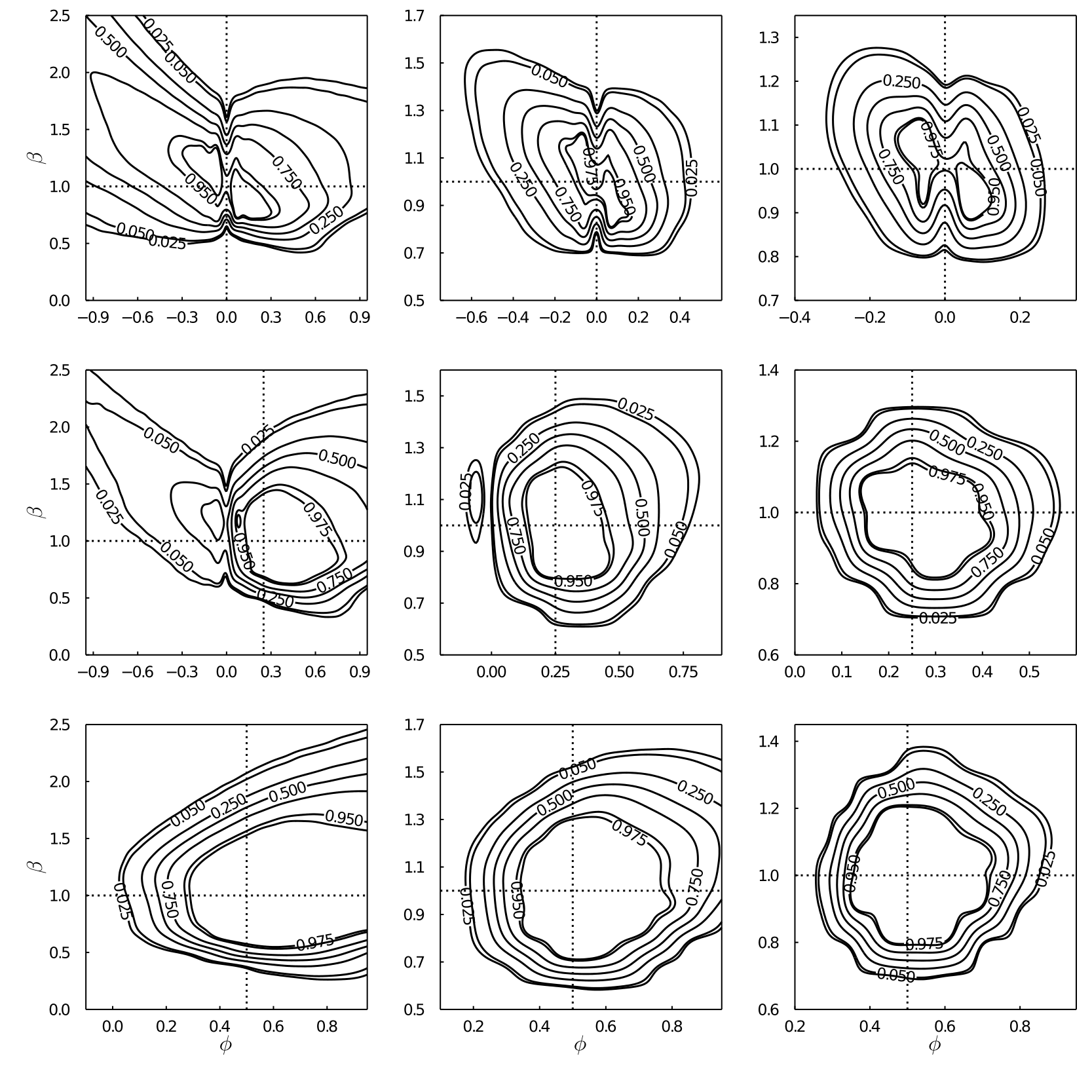
Figure 1. False Coverage Probability of the Confidence Intervals for (0,0)(\phi_{0},\beta_{0}) at 95%95\% with |G|{10,30}\left\lvert G\right\rvert\in\{10,30\}. The intersecting point between two dotted lines in each panel indicates the true parameter (0,0)(\beta_{0},\phi_{0}). The horizontal axis represents the hypothesized value of \phi and the vertical axis that of \beta. As \phi is away from the true value, the hindsight regret tends to become larger. Also, note that the (false?) coverage probability shows good performance when 0>0\phi_{0}>0 and |Ng|=300\lvert N_{g}\rvert=300 despite the fact that the coverage probabilities (are?) were 11 in Tables 4.2 and 4.2.

|G|=10,|Ng|=100|G|=30,|Ng|=100|G|=30,|Ng|=300\hskip 34.14322pt\left\lvert G\right\rvert=10,\lvert N_{g}\rvert=100\hskip 51.21504pt\left\lvert G\right\rvert=30,\lvert N_{g}\rvert=100\hskip 51.21504pt\left\lvert G\right\rvert=30,\lvert N_{g}\rvert=300 Refer to caption

4.3. Finite Sample Power of the Bootstrap Test

We saw that as 0\phi_{0} moves away from zero, the coverage probability tends to be conservative. However, as mentioned before, this does not necessarily mean that the inference will mostly be uninformative. To show this, we present results showing the finite sample power properties. We first consider inference of 0\phi_{0}. The nominal coverage probability is set to be at 95%, and the number of the information groups are set to be 1010 or 3030.

The results are shown in Figure 1. The horizontal axis represents the hypothesized value of \phi under the null hypothesis while the vertical axis that of \beta. The intersecting point between two dotted lines indicates the true parameter (0,0)(\beta_{0},\phi_{0}). We set 0=1\beta_{0}=1 and choose 0\phi_{0} from {0,1/4,1/2}\{0,1/4,1/2\}. The bootstrap results show higher false coverage probability rates as 0\phi_{0} moves away from zero, and substantial improvement as the sample size increases.

There are two notable features. First, when 0=1/4\phi_{0}=1/4 and |Ng|=300\lvert N_{g}\rvert=300, we saw that the coverage probabilities were equal to one in Tables 4.2 and 4.2, suggesting extreme conservativeness of the procedure. However, Figure 1 shows that even in this case, the false coverage probabilities are reasonably low as \phi moves away from zero. This emphasizes the fact that the conservative coverage probabilities (or conservative size properties) do not necessarily imply trivial or weak power properties in finite samples.

Second, when 0=1/2\phi_{0}=1/2, the false coverage probability at value 00 is almost zero. This means that when 0\phi_{0} is away from zero, the confidence interval has almost zero probability of covering 00. As 0\phi_{0} is away from zero, the power of the bootstrap test (testing the null hypothesis of 0=0\phi_{0}=0) naturally increases, but the moment inequalities also become more conservative. Despite this conservativeness, the bootstrap test does not lose power to detect the deviation from the null hypothesis of 0=0\phi_{0}=0. This has a significant implication in empirical applications because often we are interested in the presence of strategic interactions among the players, and 0=0\phi_{0}=0 in this context means absence of such interactions.

It is generally expected that the hindsight regret also affects the estimation of 0\beta_{0}. Figure 1 shows similar results for 0\beta_{0}. More specifically, increasing the group size |Ng|\lvert N_{g}\rvert substantially improves the false coverage probability of the confidence sets.

5. Conclusion

This paper focuses on a large Bayesian game perspective for social interactions models and develops an inference method that is robust to heterogeneous beliefs among the players. Utilizing the strategic interdependence among the players and the assumption of conditionally independent types, this work derives testable implications from the equilibrium constraints.

The framework proposed in this paper may have limitations in some applications for several reasons. First, the framework assumes that the information groups are exogenously given in the beginning of the game. This does not cause any problem, if the current game’s types satisfy the conditional independence assumption given any information used by the agents in the endogenous group formation that occurs prior to the game. However, this conditional independence assumption is violated when the agents observe the groups formed before they decide to enter the current game. Second, the framework assumes that the idiosyncratic component of the types is not shared between two different players. This assumption excludes a large network model where the information flow along connected neighborhoods. Explorations on both fronts require further research.

References

  • Andrews (2005) Andrews, D. W. K., 2005. Cross-section regression with common shocks. Econometrica 73 (5), 1551–1585.
  • Andrews and Shi (2013) Andrews, D. W. K., Shi, X., 2013. Inference based on conditional moment inequalities. Econometrica 81 (2), 609–666.
  • Andrews and Soares (2010) Andrews, D. W. K., Soares, G., 2010. Inference for parameters defined by moment inequalities using generalized moment selection. Econometrica 78 (1), 119–157.
  • Aradillas-Lopez (2010) Aradillas-Lopez, A., 2010. Semiparametric estimation of a simultaneous game with incomplete information. Journal of Econometrics 157 (2), 409–431.
  • Aradillas-Lopez and Tamer (2008) Aradillas-Lopez, A., Tamer, E., 2008. The identification power of equilibrium in simple games. Journal of Business & Economic Statistics 26 (3), 261–283.
  • Athey (2001) Athey, S., 2001. Single crossing properties and the existence of pure strategy equilibria in games of incomplete information. Econometrica 69 (4), 861–889.
  • Aumann (1976) Aumann, R. J., 11 1976. Agreeing to disagree. Ann. Statist. 4 (6), 1236–1239.
  • Bajari et al. (2010) Bajari, P., Hong, H., Krainer, J., Nekipelov, D., 2010. Estimating static models of strategic interactions. Journal of Business & Economic Statistics 28 (4), 469–482.
  • Beresteanu et al. (2011) Beresteanu, A., Molchanov, I., Molinari, F., 2011. Sharp identification regions in models with convex moment predictions. Econometrica 79 (6), 1785–1821.
  • Bergemann and Morris (2005) Bergemann, D., Morris, S., 2005. Robust mechanism design. Econometrica 73 (6), 1771–1813.
  • Bisin et al. (2011) Bisin, A., Moro, A., Topa, G., 2011. The empirical content of models with multiple equilibria in economies with social interactions. NBER Working Papers 17196, National Bureau of Economic Research, Inc.
  • Blume et al. (2011) Blume, L. E., Brock, W. A., Durlauf, S. N., Jayaraman, R., 2011. Linear social network models, working Paper.
  • Blume et al. (2015) Blume, L. E., Brock, W. A., Durlauf, S. N., Jayaraman, R., 2015. Linear social interactions models. Journal of Political Economy 123, 444–496.
  • Bresnahan and Reiss (1991) Bresnahan, T. F., Reiss, P. C., 1991. Empirical models of discrete games. Journal of Econometrics 48 (1), 57–81.
  • Brock and Durlauf (2001) Brock, W. A., Durlauf, S. N., 2001. Discrete choice with social interactions. The Review of Economic Studies 68 (2), 235–260.
  • Cameron et al. (2008) Cameron, A. C., Gelbach, J. B., Miller, D. L., 2008. Bootstrap-based improvements for inference with clustered errors. The Review of Economics and Statistics 90 (3), 414–427.
  • Canen et al. (2020) Canen, N., Schwartz, J., Song, K., 2020. Estimating local interactions among many agents who observe their neighbors. Quantitative Economics 11, 917–956.
  • Ciliberto and Tamer (2009) Ciliberto, F., Tamer, E., 2009. Market structure and multiple equilibria in airline markets. Econometrica 77 (6), 1791–1828.
  • de Paula (2013) de Paula, A., 2013. Econometric analysis of games with multiple equilibria. Annual Review of Economics 5 (1), 107–131.
  • de Paula and Tang (2012) de Paula, A., Tang, X., 2012. Inference of signs of interaction effects in simultaneous games with incomplete information. Econometrica 80 (1), 143–172.
  • Deb and Kalai (2015) Deb, J., Kalai, E., 2015. Stability in large Bayesian games with heterogeneous players. Journal of Economic Theory 157, 1041–1055.
  • Dominitz and Manski (1997) Dominitz, J., Manski, C. F., 1997. Using expectations data to study subjective income expectations. Journal of the American Statistical Association 92 (439), 855–867.
  • Ioannides (2013) Ioannides, Y. M., 2013. From Neighborhoods to Nations: The Economics of Social Interactions. Princeton University Press.
  • Ioannides and Zabel (2008) Ioannides, Y. M., Zabel, J. E., 2008. Interactions, neighborhood selection and housing demand. Journal of Urban Economics 63 (1), 229–252.
  • Jensen (1984) Jensen, D. R., 1984. Ordering ellipsoidal measures: Scale and peakness ordering. SIAM Journal on Applied Mathematics 44 (6), 1226–1231.
  • Kalai (2004) Kalai, E., 2004. Large robust games. Econometrica 72 (6), 1631–1665.
  • Kojevnikov and Song (2020) Kojevnikov, D., Song, K., 2020. On Berry-Esseen bounds for maxima of vector-valued martingales.
  • Krauth (2006) Krauth, B. V., 2006. Simulation-based estimation of peer effects. Journal of Econometrics 133 (1), 243–271.
  • Kuersteiner and Prucha (2013) Kuersteiner, G. M., Prucha, I. R., 2013. Limit theory for panel data models with cross sectional dependence and sequential exogeneity. Journal of Econometrics 174 (2), 107–126.
  • Li and Lee (2009) Li, J., Lee, L.-f., 2009. Binary choice under social interactions: An empirical study with and without subjective data on expectations. Journal of Applied Econometrics 24 (2), 257–281.
  • Manski (2004) Manski, C. F., 2004. Measuring expectations. Econometrica 72 (5), 1329–1376.
  • McAdams (2003) McAdams, D., 2003. Isotone equilibrium in games of incomplete information. Econometrica 71 (4), 1191–1214.
  • Menzel (2012) Menzel, K., 2012. Inference for large games with exchangeable players, working paper.
  • Milgrom and Weber (1985) Milgrom, P. R., Weber, R. J., 1985. Distributional strategies for games with incomplete information. Mathematics of Operations Research 10 (4), 619–632.
  • Morris (1995) Morris, S. M., 1995. The common prior assumption in economic theory. Economics and Philosopy 11, 227–253.
  • Reny (2011) Reny, P. J., 2011. On the existence of monotone pure-strategy equilibria in bayesian games. Econometrica 79 (2), 499–553.
  • Romano et al. (2014) Romano, J. P., Shaikh, A. M., Wolf, M., 2014. A practical two-step method for testing moment inequalities. Econometrica 82 (5), 1979–2002.
  • Rosen (2008) Rosen, A. M., 2008. Confidence sets for partially identified parameters that satisfy a finite number of moment inequalities. Journal of Econometrics 146 (1), 107–117.
  • Tamer (2003) Tamer, E., 01 2003. Incomplete simultaneous discrete response model with multiple equilibria. The Review of Economic Studies 70 (1), 147–165.
  • Wilson (1987) Wilson, R., 1987. Game-Theoretic Analyses of Trading Processes. Econometric Society Monographs. Cambridge University Press, pp. 33–70.
  • Xu (2018) Xu, H., 2018. Social interactions in large networks: A game theoretic approach. International Economic Review 59 (1), 257–284.

Appendix A Extension to Multinomial Action Sets

In this appendix we show how the results of the main text can be extended to the case with a multinomial action set, i.e., k:=|A|>2k:=\left\lvert A\right\rvert>2. The formal result in this appendix include Theorem 3.1 as a special case. Throughout the appendix, an inequality between two vectors x=[xj]x=[x_{j}] and y=[yj]y=[y_{j}], say, xyx\geq y, represents the corresponding elementwise inequalities, i.e., xjyjx_{j}\geq y_{j} for all jj. The proofs of the results in Appendix A appear in Appendix B below.

A.1. Belief-free Hindsight Regrets

For iNi\in N and a,aAa,a^{\prime}\in A, we define

ui(a,a,b,t):=ui(a,b,t)ui(a,b,t)u_{i}^{\Delta}(a,a^{\prime},b;t):=u_{i}(a,b;t)-u_{i}(a^{\prime},b;t)

which is player ii’s payoff differential between choosing aa and aa^{\prime} when the other players choose bAn1b\in A^{n-1}, n=|N|n=|N|.

Definition A.1.

Given an equilibrium 𝒴\mathcal{Y} and (0,1)\rho\in(0,1), an i\mathcal{I}_{i}-measurable random vector [0,)k1\boldsymbol{\lambda}\in[0,\infty)^{k-1} is a \rho-hindsight regret for player iNi\in N if

𝖰i(𝐮i(Yi,Yi,i)>i)1(𝖰i-a.s.),\mathsf{Q}_{i}\left(\mathbf{u}_{i}^{\Delta}(Y_{i},Y_{-i};\tau_{i})>-\boldsymbol{\lambda}\mid\mathcal{I}_{i}\right)\geq 1-\rho\quad(\mathsf{Q}_{i}\text{-a.s.}),

where 𝐮i(a,b,t):=[ui(a,a,b,t)]aA{a}\mathbf{u}_{i}^{\Delta}(a,b;t):=[u_{i}^{\Delta}(a,a^{\prime},b;t)]_{a^{\prime}\in A\setminus\{a\}}.

Let 𝒊,(a,t):=[i,(a,a,t)]aA{a}\boldsymbol{\lambda_{i,\rho}}(a,t):=[\lambda_{i,\rho}(a,a^{\prime},t)]_{a^{\prime}\in A\setminus\{a\}} be a vector in 𝐑k1\mathbf{R}^{k-1} whose elements are given by

(A.1) i,(a,a,t):=12ln(k1)i(a,a,t),\displaystyle\lambda_{i,\rho}(a,a^{\prime},t):=\sqrt{-\frac{1}{2}\ln\left(\frac{\rho}{k-1}\right)\cdot\Lambda_{i}(a,a^{\prime},t)},

where

i(a,a,t):=jN{i}Vj2(ui(a,a,;t)),\Lambda_{i}(a,a^{\prime},t):=\sum_{j\in N\setminus\{i\}}V_{j}^{2}(u_{i}^{\Delta}(a,a^{\prime},\cdot;t)),

and Vj()V_{j}(\,\cdot\,) denotes the maximal variation defined in (2.6).

The following theorem confirms that 𝒊,(Yi,i)\boldsymbol{\lambda_{i,\rho}}(Y_{i},\tau_{i}) is a \rho-hindsight regret.

Theorem A.1.

Suppose that Assumptions 2.1 and 2.2 hold. Then for any pure strategy equilibrium 𝒴\mathcal{Y}, i,(Yi,i)\boldsymbol{\lambda}_{i,\rho}(Y_{i},\tau_{i}) is a \rho-hindsight regret for player iNi\in N. Moreover,

𝖯(𝐮i(Yi,Yi,i)>i,(Yi,i)i)1i(Yi,i)(𝖯-a.s.),\mathsf{P}\left(\mathbf{u}_{i}^{\Delta}(Y_{i},Y_{-i};\tau_{i})>-\boldsymbol{\lambda}_{i,\rho}(Y_{i},\tau_{i})\mid\mathcal{I}_{i}\right)\geq 1-\rho_{i}(Y_{i},\tau_{i})\quad(\mathsf{P}\text{-a.s.}),

where

i(a,t):=k1aA{a}1{i,(a,a,t)>0}.\rho_{i}(a,t):=\frac{\rho}{k-1}\sum_{a^{\prime}\in A\setminus\{a\}}1\{\lambda_{i,\rho}(a,a^{\prime},t)>0\}.

A.2. Testable Implications

First, for each iNi\in N and aAa\in A, we construct i,L(a):=i,L(a,Xi,Yi)\pi_{i,L}(a):=\pi_{i,L}(a,X_{i},Y_{-i}) and i,U(a):=i,U(a,Xi,Yi)\pi_{i,U}(a):=\pi_{i,U}(a,X_{i},Y_{-i}) which can be simulated as follows:

i,L(a,x,b)\displaystyle\pi_{i,L}(a,x,b) =𝖯(iHi,L(a,x,b)Xi=x)and\displaystyle=\mathsf{P}\left(\eta_{i}\in H_{i,L}(a,x,b)\mid X_{i}=x\right)\quad\text{and}
i,U(a,x,b)\displaystyle\pi_{i,U}(a,x,b) =𝖯(iHi,U(a,x,b)Xi=x),\displaystyle=\mathsf{P}\left(\eta_{i}\in H_{i,U}(a,x,b)\mid X_{i}=x\right),

where, letting t(x,)t\equiv(x,\eta),

Hi,L(a,x,b)\displaystyle H_{i,L}(a,x,b) :={𝐑w:aA{a} s.t. 𝐮i(a,b;t)>i,(a,t)}and\displaystyle:=\left\{\eta\in\mathbf{R}^{w}:\exists a^{\prime}\in A\setminus\{a\}\text{ s.t. }\mathbf{u}_{i}^{\Delta}(a^{\prime},b;t)>-\boldsymbol{\lambda}_{i,\rho}(a^{\prime},t)\right\}\quad\text{and}
Hi,U(a,x,b)\displaystyle H_{i,U}(a,x,b) :={𝐑w:𝐮i(a,b,t)>i,(a,t)}.\displaystyle:=\left\{\eta\in\mathbf{R}^{w}:\mathbf{u}_{i}^{\Delta}(a,b;t)>-\boldsymbol{\lambda}_{i,\rho}(a,t)\right\}.

Indeed, by Assumption 3.1(b), i\eta_{i} is conditionally independent of YiY_{-i} given XiX_{i}. Hence, we can simulate i,L(a,x,b)\pi_{i,L}(a,x,b) and i,U(a,x,b)\pi_{i,U}(a,x,b) by drawing i\eta_{i}’s from the conditional distribution Fi,(x)F_{i,\theta}(\,\cdot\,\mid x) in Assumption 3.2.

For each aAa\in A, we define

(A.2) ei,L(a):=𝟏{Yi=a}(1i,L(a)1i,L(a))andei,U(a):=𝟏{Yi=a}i,U(a)1i,U(a),\displaystyle\begin{aligned} e_{i,L}(a):=&\mathbf{1}\{Y_{i}=a\}-\left(1-\frac{\pi_{i,L}(a)}{1-\rho_{i,L}(a)}\right)\quad\text{and}\\ e_{i,U}(a):=&\mathbf{1}\{Y_{i}=a\}-\frac{\pi_{i,U}(a)}{1-\rho_{i,U}(a)},\end{aligned}

where

i,L(a)\displaystyle\rho_{i,L}(a) :=𝟏{maxc,aA{a}supti,(c,a,t)>0}and\displaystyle:=\rho\cdot\mathbf{1}\left\{\max_{c,a^{\prime}\in A\setminus\{a\}}\sup_{t}\lambda_{i,\rho}(c,a^{\prime},t)>0\right\}\quad\text{and}
i,U(a)\displaystyle\rho_{i,U}(a) :=𝟏{maxaA{a}supti,(a,a,t)>0}.\displaystyle:=\rho\cdot\mathbf{1}\left\{\max_{a^{\prime}\in A\setminus\{a\}}\sup_{t}\lambda_{i,\rho}(a,a^{\prime},t)>0\right\}.

Let 𝐞i,L\mathbf{e}_{i,L} and 𝐞i,U\mathbf{e}_{i,U} be vectors of dimension k1k-1 whose elements are ei,L(a)e_{i,L}(a) and ei,U(a)e_{i,U}(a) with aa running in A{a1}A\setminus\{a_{1}\}. Choosing a vector of non-negative measurable functions 𝐠i:=[gi,1,,gi,m]:𝐑v[0,)m\mathbf{g}_{i}:=[g_{i,1},\ldots,g_{i,m}]^{\top}:\mathbf{R}^{v}\to[0,\infty)^{m}, we define sample moments as follows

(A.3) ^L:=1niN𝐞i,L𝐠i(Xi)and^U:=1niN𝐞i,U𝐠i(Xi),\displaystyle\boldsymbol{\hat{\mu}}_{L}:=\frac{1}{n}\sum_{i\in N}\mathbf{e}_{i,L}\otimes\mathbf{g}_{i}(X_{i})\quad\text{and}\quad\boldsymbol{\hat{\mu}}_{U}:=\frac{1}{n}\sum_{i\in N}\mathbf{e}_{i,U}\otimes\mathbf{g}_{i}(X_{i}),

where \otimes denotes the Kronecker product. The following result establishes the moment inequalities as testable implications.

Proposition A.1.

Suppose that Assumptions 2.1-3.2 are satisfied. Then

L0andU0(𝖯-a.s.),\displaystyle\boldsymbol{\mu}_{L}\geq 0\quad\text{and}\quad\boldsymbol{\mu}_{U}\leq 0\quad(\mathsf{P}\text{-a.s.}),

where

(A.4) L:=𝖤P[^L]andU:=𝖤P[^U].\displaystyle\begin{aligned} \boldsymbol{\mu}_{L}:=\mathsf{E}_{P}[\boldsymbol{\hat{\mu}}_{L}\mid\mathcal{F}]\quad\text{and}\quad\boldsymbol{\mu}_{U}:=\mathsf{E}_{P}[\boldsymbol{\hat{\mu}}_{U}\mid\mathcal{F}].\end{aligned}

A.3. Bootstrap Inference

A.3.1. Test Statistic

Using the sample moments, we take the following as our test statistic:

(A.5) T:=𝒯(n(^L+𝐰L),n(^U𝐰U)),\displaystyle T:=\mathcal{T}\left(\sqrt{n}(\boldsymbol{\hat{\mu}}_{L}+\mathbf{w}_{L}),\sqrt{n}(\boldsymbol{\hat{\mu}}_{U}-\mathbf{w}_{U})\right),

where 𝒯:𝐑d×𝐑d𝐑\mathcal{T}:\mathbf{R}^{d}\times\mathbf{R}^{d}\to\mathbf{R} is a function defined by 𝒯(x,y):=[x]+[y]+1\mathcal{T}(x,y):=\left\lVert[x]_{-}+[y]_{+}\right\rVert_{1}, and 𝐰L\mathbf{w}_{L} and 𝐰U\mathbf{w}_{U} are constructed as follows. For jij\neq i, 1lm1\leq l\leq m, and aAa\in A, let

(A.6) dl,L(a)\displaystyle d_{l,L}(a) :=1njNiN{j}V(i,j)(i,L(a,Xi,))gi,l(Xi)1i,L(a)and\displaystyle:=\frac{1}{n}\sum_{j\in N}\sum_{i\in N\setminus\{j\}}\frac{V_{\sigma(i,j)}(\pi_{i,L}(a,X_{i},\,\cdot\,))g_{i,l}(X_{i})}{1-\rho_{i,L}(a)}\quad\text{and}
dl,U(a)\displaystyle d_{l,U}(a) :=1njNiN{j}V(i,j)(i,U(a,Xi,))gi,l(Xi)1i,U(a),\displaystyle:=\frac{1}{n}\sum_{j\in N}\sum_{i\in N\setminus\{j\}}\frac{V_{\sigma(i,j)}(\pi_{i,U}(a,X_{i},\,\cdot\,))g_{i,l}(X_{i})}{1-\rho_{i,U}(a)},

where (i,j)\sigma(i,j) is the index of the jj-th element of N{i}N\setminus\{i\}. Then for a given %(0,1)\varrho\in(0,1), the elements of 𝐰L\mathbf{w}_{L} are defined to be

12ln(%4d)dl,L2(a),\sqrt{-\frac{1}{2}\ln\left(\frac{\varrho}{4d}\right)d_{l,L}^{2}(a)},

with aa running in A{a1}A\setminus\{a_{1}\} and ll running in {1,,m}\{1,\ldots,m\}, keeping the same order of elements as in the sample moments ^L\boldsymbol{\hat{\mu}}_{L} and ^U\boldsymbol{\hat{\mu}}_{U}. The elements of 𝐰U\mathbf{w}_{U} are defined similarly, with dl,L(a)d_{l,L}(a) replaced by dl,U(a)d_{l,U}(a).

A.3.2. Bootstrap Critical Values

As for the bootstrap statistic, we draw i.i.d. standard normal random variables {"1,,"n}\{\varepsilon_{1},\ldots,\varepsilon_{n}\} and take

(A.7) :=1niN((𝐘ii)𝐠i(Xi))"i,\displaystyle\boldsymbol{\zeta}^{*}:=\frac{1}{n}\sum_{i\in N}\left((\mathbf{Y}_{i}-\boldsymbol{\mu}_{i}^{*})\otimes\mathbf{g}_{i}(X_{i})\right)\varepsilon_{i},

where 𝐘i\mathbf{Y}_{i} and i\boldsymbol{\mu}_{i}^{*} are column vectors formed by 𝟏{Yi=a}\mathbf{1}\{Y_{i}=a\} and

(12(1i,L(a)i,U(a)1i(a))0)1,\left(\frac{1}{2}\left(1-\frac{\pi_{i,L}(a)-\pi_{i,U}(a)}{1-\rho_{i}(a)}\right)\vee 0\right)\wedge 1,

respectively, with aa running in A{a1}A\setminus\{a_{1}\}. In addition, given fixed (0,1)\kappa\in(0,1), we define

'^L\displaystyle\boldsymbol{\hat{\varphi}}_{L} :=[^L𝐰L𝟏dq(1/2)/n]+and\displaystyle:=\left[\boldsymbol{\hat{\mu}}_{L}-\mathbf{w}_{L}-\mathbf{1}_{d}\cdot q^{*}(1-\kappa/2)/\sqrt{n}\right]_{+}\quad\text{and}
'^U\displaystyle\boldsymbol{\hat{\varphi}}_{U} :=[^U+𝐰U+𝟏dq(1/2)/n],\displaystyle:=\left[\boldsymbol{\hat{\mu}}_{U}+\mathbf{w}_{U}+\mathbf{1}_{d}\cdot q^{*}(1-\kappa/2)/\sqrt{n}\right]_{-},

where q(1/2)q^{*}(1-\kappa/2) is the (1/2)(1-\kappa/2) quantile of the bootstrap distribution of n\sqrt{n}\|\boldsymbol{\zeta}^{*}\|_{\infty}.

We consider the following bootstrap test statistic:

(A.8) T:=𝒯(n(+'^L'^U),n('^L'^U)),\displaystyle T^{*}:=\mathcal{T}\left(\sqrt{n}(\boldsymbol{\zeta}^{*}+\boldsymbol{\hat{\varphi}}_{L}\wedge\boldsymbol{\hat{\varphi}}_{U}),\sqrt{n}(\boldsymbol{\zeta}^{*}-\boldsymbol{\hat{\varphi}}_{L}\wedge\boldsymbol{\hat{\varphi}}_{U})\right),

(the minimum between '^L\boldsymbol{\hat{\varphi}}_{L} and '^U\boldsymbol{\hat{\varphi}}_{U} is taken element-wise). The confidence set for 0\theta_{0}\in\Theta at nominal level 11-\alpha is given by

CS:={:Tc( )},CS_{\epsilon}:=\{\theta\in\Theta:T\leq c^{*}(\gamma)\vee\epsilon\},

where >0\epsilon>0 is a fixed small number and c( )c^{*}(\gamma) is the :=(1+%+)\gamma:=(1-\alpha+\varrho+\kappa)-quantile of the bootstrap distribution of TT^{*}.

Theorem A.2.

Suppose that Assumptions 1-4 hold and there exists C𝐠>0C_{\mathbf{g}}>0 such that for all n1n\geq 1, maxiNmax1lmgilC𝐠\max_{i\in N}\max_{1\leq l\leq m}\left\lVert g_{il}\right\rVert_{\infty}\leq C_{\mathbf{g}}. Furthermore, assume that there exists a positive sequence {rn}\{r_{n}\} such that rn1=O(n1/(3+))r_{n}^{-1}=O(n^{1/(3+\delta)}) for some >0\delta>0 and

(A.9) limnsup𝖯𝒫0𝖯(¯(V)<rn)=0.\displaystyle\lim_{n\to\infty}\sup_{\mathsf{P}\in\mathcal{P}_{0}}\mathsf{P}\left(\underline{\lambda}(V)<r_{n}\right)=0.

Then for a positive sequence {n}\{\epsilon_{n}\} such that n1=o(n1/8)\epsilon_{n}^{-1}=o(n^{1/8}),

lim supnsup𝖯𝒫0𝖯(0CSn).\limsup_{n\to\infty}\sup_{\mathsf{P}\in\mathcal{P}_{0}}\mathsf{P}\left(\theta_{0}\notin CS_{\epsilon_{n}}\right)\leq\alpha.

Appendix B Proofs of the Main Results

B.1. Proofs

Throughout the proofs, we use notation C,C,C′′C,C^{\prime},C^{\prime\prime}, etc., to denote positive constants that depend only on dd, mm, kk and C𝐠C_{\mathbf{g}} in Theorem A.2. We will refer to them as “absolute constants” throughout the proofs.

First, for aAa\in A, let

(B.1) e~i,L(a):=𝟏{Yi=a}(1𝖤𝖯[i,L(a)]1i(a))ande~i,U(a):=𝟏{Yi=a}𝖤𝖯[i,U(a)]1i(a),\displaystyle\begin{aligned} \tilde{e}_{i,L}(a):=&\mathbf{1}\{Y_{i}=a\}-\left(1-\frac{\mathsf{E}_{\mathsf{P}}[\pi_{i,L}(a)\mid\mathcal{F}]}{1-\rho_{i}(a)}\right)\quad\text{and}\\ \tilde{e}_{i,U}(a):=&\mathbf{1}\{Y_{i}=a\}-\frac{\mathsf{E}_{\mathsf{P}}[\pi_{i,U}(a)\mid\mathcal{F}]}{1-\rho_{i}(a)},\end{aligned}

and let 𝐞~i,L\mathbf{\tilde{e}}_{i,L} and 𝐞~i,U\mathbf{\tilde{e}}_{i,U} be column vectors whose elements are e~i,L(a)\tilde{e}_{i,L}(a) and e~i,U(a)\tilde{e}_{i,U}(a) with aa running in A{a1}A\setminus\{a_{1}\}. The infeasible moments are given by

(B.2) ~L:=1niN𝐞~i,L𝐠i(Xi)and~U:=1niN𝐞~i,U𝐠i(Xi).\displaystyle\boldsymbol{\tilde{\mu}}_{L}:=\frac{1}{n}\sum_{i\in N}\mathbf{\tilde{e}}_{i,L}\otimes\mathbf{g}_{i}(X_{i})\quad\text{and}\quad\boldsymbol{\tilde{\mu}}_{U}:=\frac{1}{n}\sum_{i\in N}\mathbf{\tilde{e}}_{i,U}\otimes\mathbf{g}_{i}(X_{i}).

The following proposition implies that the difference between the feasible and infeasible moments are controlled by 𝐰L\mathbf{w}_{L} and 𝐰U\mathbf{w}_{U} with a large probability.

Proposition B.1.

Suppose that Assumptions 2.1-3.2 hold, and 𝐰L\mathbf{w}_{L} and 𝐰U\mathbf{w}_{U} are constructed using (A.6) as in Section A.3.1. Then,

𝖯(|^L~L|𝐰L,|^U~U|𝐰U)1%,\mathsf{P}\left(\lvert\boldsymbol{\hat{\mu}}_{L}-\boldsymbol{\tilde{\mu}}_{L}\rvert\leq\mathbf{w}_{L},\lvert\boldsymbol{\hat{\mu}}_{U}-\boldsymbol{\tilde{\mu}}_{U}\rvert\leq\mathbf{w}_{U}\right)\geq 1-\varrho,

where for a vector x=[xj]x=[x_{j}], |x|=[|xj|]\left\lvert x\right\rvert=[|x_{j}|], and the inequalities above are elementwise.

Proof.

Since the elements of YiY_{-i} are conditionally independent given \mathcal{F} by Assumption 2.1, the result follows from the definition of 𝐰L\mathbf{w}_{L} and 𝐰U\mathbf{w}_{U} and Lemma C.1 in the supplemental note. ∎

Proof of Theorem A.1.

First, note that YiY_{i} and i\tau_{i} are i\mathcal{I}_{i}-measurable and the elements of YiY_{-i} are conditionally independent given i\mathcal{I}_{i} by Assumption 2.1. The assertions of the theorem follow from Lemma C.1 in the supplemental note and Assumption 2.2. ∎

Proof of Proposition A.1.

For aAa\in A, define the events

Si,U(a):={𝐮i(a,Yi;i)>i,(a,i)}andSi,L(a):=aA{a}Si,U(a).S_{i,U}(a):=\{\mathbf{u}_{i}^{\Delta}(a,Y_{-i};\tau_{i})>-\boldsymbol{\lambda}_{i,\rho}(a,\tau_{i})\}\quad\text{and}\quad S_{i,L}(a):=\bigcup_{a^{\prime}\in A\setminus\{a\}}S_{i,U}(a^{\prime}).

By the definition of i,\boldsymbol{\lambda}_{i,\rho} and Theorem A.1 we have

(B.3) aA𝖯(Si,U(a)i)𝟏{Yi=a}1aAi(a,i)𝟏{Yi=a}(𝖯-a.s.).\displaystyle\sum_{a\in A}\mathsf{P}\left(S_{i,U}(a)\mid\mathcal{I}_{i}\right)\mathbf{1}\{Y_{i}=a\}\geq 1-\sum_{a\in A}\rho_{i}(a,\tau_{i})\mathbf{1}\{Y_{i}=a\}\quad(\mathsf{P}\text{-a.s.}).

Therefore, noticing that i(a,i)i,U(a)\rho_{i}(a,\tau_{i})\leq\rho_{i,U}(a),

(B.4) 𝟏{Yi=a}𝟏{𝖯(Si,U(a)i)1i,U(a)}(𝖯-a.s.).\displaystyle\mathbf{1}\{Y_{i}=a\}\leq\mathbf{1}\left\{\mathsf{P}\left(S_{i,U}(a)\mid\mathcal{I}_{i}\right)\geq 1-\rho_{i,U}(a)\right\}\quad(\mathsf{P}\text{-a.s.}).

On the other hand, note that the events Si,U(a)S_{i,U}(a) and Si,U(a)S_{i,U}(a^{\prime}) with aaa\neq a^{\prime} are disjoint because i,(a,a,t)=i,(a,a,t)\lambda_{i,\rho}(a,a^{\prime},t)=\lambda_{i,\rho}(a^{\prime},a,t). (Recall the definition in (A.1).) Hence, from (B.3),

(B.5) 𝟏{Yia}\displaystyle\mathbf{1}\{Y_{i}\neq a\} 𝟏{𝖯(Si,L(a)i)1i,L(a)}(𝖯-a.s.).\displaystyle\leq\mathbf{1}\left\{\mathsf{P}\left(S_{i,L}(a)\mid\mathcal{I}_{i}\right)\geq 1-\rho_{i,L}(a)\right\}\quad(\mathsf{P}\text{-a.s.}).

Taking the conditional expectations w.r.t. \mathcal{F} on both sides of the inequalities in (B.4) and (B.5), using Markov’s inequality, and noticing that \mathcal{F} is a sub \sigma-field of i\mathcal{I}_{i} for all iNi\in N, we find that

𝖯(Yi=a)\displaystyle\mathsf{P}\left(Y_{i}=a\mid\mathcal{F}\right) (1i,U(a))1𝖯(Si,U(a))(𝖯-a.s.)and\displaystyle\leq(1-\rho_{i,U}(a))^{-1}\mathsf{P}\left(S_{i,U}(a)\mid\mathcal{F}\right)\quad(\mathsf{P}\text{-a.s.})\quad\text{and}
𝖯(Yia)\displaystyle\mathsf{P}\left(Y_{i}\neq a\mid\mathcal{F}\right) (1i,L(a))1𝖯(Si,L(a))(𝖯-a.s.).\displaystyle\leq(1-\rho_{i,L}(a))^{-1}\mathsf{P}\left(S_{i,L}(a)\mid\mathcal{F}\right)\quad(\mathsf{P}\text{-a.s.}).

These inequalities give the desired result. ∎

Proof of Theorem A.2.

Let 𝒢:=(Y1,,Yn)\mathcal{G}:=\mathcal{F}\vee\sigma(Y_{1},\ldots,Y_{n}) and let

(B.6) :=1niN(𝐘i𝖤𝖯[𝐘i])𝐠i(Xi),\displaystyle\boldsymbol{\zeta}:=\frac{1}{n}\sum_{i\in N}(\mathbf{Y}_{i}-\mathsf{E}_{\mathsf{P}}[\mathbf{Y}_{i}\mid\mathcal{F}])\otimes\mathbf{g}_{i}(X_{i}),

so that we have

(B.7) =~LL=~UU(𝖯-a.s.).\displaystyle\boldsymbol{\zeta}=\boldsymbol{\tilde{\mu}}_{L}-\boldsymbol{\mu}_{L}=\boldsymbol{\tilde{\mu}}_{U}-\boldsymbol{\mu}_{U}\quad(\mathsf{P}\text{-a.s.}).

Under Assumption 2.1, Y1,,YnY_{1},\ldots,Y_{n} are conditionally independent given \mathcal{F}. It follows that \boldsymbol{\zeta} is the sum of conditionally independent random vectors given \mathcal{F}.

Let ZZ be a standard normal random vector in 𝐑d\mathbf{R}^{d} independent of 𝒢\mathcal{G}. Define

(B.8) T~:=𝒯(n~L,n~U)andT~:=𝒯(n(+L(U)),n(L(U))).\displaystyle\begin{aligned} \widetilde{T}&:=\mathcal{T}\left(\sqrt{n}\boldsymbol{\tilde{\mu}}_{L},\sqrt{n}\boldsymbol{\tilde{\mu}}_{U}\right)\quad\text{and}\\ \widetilde{T}^{\prime}&:=\mathcal{T}\left(\sqrt{n}(\boldsymbol{\zeta}+\boldsymbol{\mu}_{L}\wedge(-\boldsymbol{\mu}_{U})),\sqrt{n}(\boldsymbol{\zeta}-\boldsymbol{\mu}_{L}\wedge(-\boldsymbol{\mu}_{U}))\right).\end{aligned}

We also introduce the following functionals of the random vector ZZ:

S\displaystyle S^{\prime} :=𝒯(V1/2Z+n(L(U)),V1/2Zn(L(U)))and\displaystyle:=\mathcal{T}\left(V^{1/2}Z+\sqrt{n}(\boldsymbol{\mu}_{L}\wedge(-\boldsymbol{\mu}_{U})),V^{1/2}Z-\sqrt{n}(\boldsymbol{\mu}_{L}\wedge(-\boldsymbol{\mu}_{U}))\right)\quad\text{and}
S\displaystyle S^{*} :=𝒯(W1/2Z+n(L(U)),W1/2Zn(L(U))),\displaystyle:=\mathcal{T}\left(W^{1/2}Z+\sqrt{n}(\boldsymbol{\mu}_{L}\wedge(-\boldsymbol{\mu}_{U})),W^{1/2}Z-\sqrt{n}(\boldsymbol{\mu}_{L}\wedge(-\boldsymbol{\mu}_{U}))\right),

where VV and WW are versions of n𝖤𝖯[]n\mathsf{E}_{\mathsf{P}}\left[\boldsymbol{\zeta}\boldsymbol{\zeta}^{\top}\mid\mathcal{F}\right] and

1niN𝖤𝖯[((𝐘ii)𝐠i(Xi))((𝐘ii)𝐠i(Xi))],\displaystyle\frac{1}{n}\sum_{i\in N}\mathsf{E}_{\mathsf{P}}\left[\left((\mathbf{Y}_{i}-\boldsymbol{\mu}_{i}^{*})\otimes\mathbf{g}_{i}(X_{i})\right)\left((\mathbf{Y}_{i}-\boldsymbol{\mu}_{i}^{*})\otimes\mathbf{g}_{i}(X_{i})\right)^{\top}\mid\mathcal{F}\right],

respectively. (Recall the definition of i\boldsymbol{\mu}_{i}^{*} after (A.7).) Let c(z)c(z) denote the zz-quantile of the conditional distribution of SS^{\prime} given \mathcal{F}, and let q(z)q(z) denote the zz-quantile of the conditional distribution of W1/2Z\|W^{1/2}Z\|_{\infty} given \mathcal{F}.

For random variables XX and YY and sub-\sigma-fields ,′′\mathcal{F}^{\prime},\mathcal{F}^{\prime\prime}\subset\mathcal{H}, we define

(B.9) dKz(X,Y,′′):=suptz|FX(t)FY(t′′)|,d_{K}^{\,z}\left(X,Y\mid\mathcal{F}^{\prime},\mathcal{F}^{\prime\prime}\right):=\sup_{t\geq z}\,\left\lvert F_{X}(t\mid\mathcal{F}^{\prime})-F_{Y}(t\mid\mathcal{F}^{\prime\prime})\right\rvert,

where FX()F_{X}(\,\cdot\,\mid\mathcal{F}^{\prime}) and FY(′′)F_{Y}(\,\cdot\,\mid\mathcal{F}^{\prime\prime}) are the conditional cdfs of XX and YY given \mathcal{F}^{\prime} and ′′\mathcal{F}^{\prime\prime}, respectively (when =′′\mathcal{F}^{\prime}=\mathcal{F}^{\prime\prime} we denote this measure by dKz(X,Y)d_{K}^{\,z}\left(X,Y\mid\mathcal{F}^{\prime}\right); also we drop the superscript zz when the supremum is taken over 𝐑\mathbf{R}). Define

(B.10) T~:=𝒯(n(+L(U)),n(L(U)))\widetilde{T}^{*}:=\mathcal{T}\left(\sqrt{n}(\boldsymbol{\zeta}^{*}+\boldsymbol{\mu}_{L}\wedge(-\boldsymbol{\mu}_{U})),\sqrt{n}(\boldsymbol{\zeta}^{*}-\boldsymbol{\mu}_{L}\wedge(-\boldsymbol{\mu}_{U}))\right)

and let c~( )\tilde{c}^{*}(\gamma) denote the \gamma-quantile of the bootstrap distribution of T~\widetilde{T}^{*}. We let

\displaystyle\Delta :=dK(T~,S𝒢,)and\displaystyle:=d_{K}^{\,\epsilon}\left(\widetilde{T}^{*},S^{*}\mid\mathcal{G},\mathcal{F}\right)\quad\text{and}
~\displaystyle\tilde{\Delta} :=dK(,W1/2Z𝒢,).\displaystyle:=d_{K}^{\,\epsilon}\left(\|\boldsymbol{\zeta}^{*}\|_{\infty},\|W^{1/2}Z\|_{\infty}\mid\mathcal{G},\mathcal{F}\right).
Claim B.1.

WVW-V is positive semidefinite (𝖯-a.s.)(\mathsf{P}\text{-a.s.}).

Proof.

Since YiY_{i}’s are conditionally independent given \mathcal{F}, i\boldsymbol{\mu}_{i}^{*}’s are \mathcal{F}-measurable, we can write

W=V+1niN𝖤𝖯[((𝖤𝖯[𝐘i]i)𝐠i(Xi))((𝖤𝖯[𝐘i]i)𝐠i(Xi))](𝖯-a.s.).W=V+\frac{1}{n}\sum_{i\in N}\mathsf{E}_{\mathsf{P}}\left[\left((\mathsf{E}_{\mathsf{P}}[\mathbf{Y}_{i}\mid\mathcal{F}]-\boldsymbol{\mu}_{i}^{*})\otimes\mathbf{g}_{i}(X_{i})\right)\left((\mathsf{E}_{\mathsf{P}}[\mathbf{Y}_{i}\mid\mathcal{F}]-\boldsymbol{\mu}_{i}^{*})\otimes\mathbf{g}_{i}(X_{i})\right)^{\top}\mid\mathcal{F}\right]\quad(\mathsf{P}\text{-a.s.}).

This gives the desired result. ∎

Claim B.2.

For any 𝖯𝒫0\mathsf{P}\in\mathcal{P}_{0} and (0, )\upsilon\in(0,\gamma),

(B.11) 𝖯(c( )>c~( ))Cbnand𝖯(q(1/2)>q(1/2))Cbn,\displaystyle\begin{aligned} \mathsf{P}\left(c(\gamma-\upsilon)>\tilde{c}^{*}(\gamma)\vee\epsilon\right)&\leq Cb_{n}\quad\text{and}\\ \mathsf{P}\left(q(1-\kappa/2-\upsilon)>q^{*}(1-\kappa/2)\right)&\leq Cb_{n},\end{aligned}

where C>0C>0 is an absolute constant and

bn:=1(rn2n)1/6+13n+𝖯(¯(V)<rn).b_{n}:=\frac{1}{\upsilon(r_{n}^{2}n)^{1/6}}+\frac{1}{\upsilon\epsilon^{3}\sqrt{n}}+\frac{\mathsf{P}\left(\underline{\lambda}(V)<r_{n}\right)}{\upsilon}.
Proof.

We first prove the first inequality in (B.11). Since WVW-V is positive semidefinite by Claim B.1, and sets of the form {x𝐑d:𝒯(x+a,xa)t}\{x\in\mathbf{R}^{d}:\mathcal{T}(x+a,x-a)\leq t\} with a[0,)da\in[0,\infty)^{d} and t0t\geq 0 are convex and symmetric under reflection, Theorem 1 in Jensen (1984) implies that for all t𝐑t\in\mathbf{R},

(B.12) 𝖯(St)𝖯(St)(𝖯-a.s.).\displaystyle\mathsf{P}\left(S^{\prime}\leq t\mid\mathcal{F}\right)\geq\mathsf{P}\left(S^{*}\leq t\mid\mathcal{F}\right)\quad(\mathsf{P}\text{-a.s.}).

On the event {}{c( )>}\{\Delta\leq\upsilon\}\cap\{c(\gamma-\upsilon)>\epsilon\},

𝖯(Sc~( )𝒢)𝖯(Sc~( )𝒢)\displaystyle\mathsf{P}\left(S^{\prime}\leq\tilde{c}^{*}(\gamma)\vee\epsilon\mid\mathcal{G}\right)\geq\mathsf{P}\left(S^{*}\leq\tilde{c}^{*}(\gamma)\vee\epsilon\mid\mathcal{G}\right)
𝖯(T~c~( )𝒢)\displaystyle\qquad\geq\mathsf{P}\left(\widetilde{T}^{*}\leq\tilde{c}^{*}(\gamma)\vee\epsilon\mid\mathcal{G}\right)-\upsilon
=𝖯(Sc( )𝒢)(𝖯-a.s.),\displaystyle\qquad\geq\gamma-\upsilon=\mathsf{P}\left(S^{\prime}\leq c(\gamma-\upsilon)\mid\mathcal{G}\right)\quad(\mathsf{P}\text{-a.s.}),

which implies that c~( )c( )\tilde{c}^{*}(\gamma)\vee\epsilon\geq c(\gamma-\upsilon). Hence, we obtain that

𝖯(c( )>c~( ))𝖯(>)(𝖯-a.s.).\mathsf{P}\left(c(\gamma-\upsilon)>\tilde{c}^{*}(\gamma)\vee\epsilon\mid\mathcal{F}\right)\leq\mathsf{P}\left(\Delta>\upsilon\mid\mathcal{F}\right)\quad(\mathsf{P}\text{-a.s.}).

Since 𝐘i,,𝐘n\mathbf{Y}_{i},\ldots,\mathbf{Y}_{n} are conditionally independent given \mathcal{F},1010 10 Here, for a given matrix A=[aij]A=[a_{ij}], Ae,1\|A\|_{e,1} denotes the elementwise 1\ell_{1} norm, i.e., Ae,1=i,j|aij|\|A\|_{e,1}=\sum_{i,j}|a_{ij}|, and Ae,\|A\|_{e,\infty} denotes the elementwise sup-norm, i.e., Ae,=maxi,j|aij|\|A\|_{e,\infty}=\max_{i,j}|a_{ij}|.

H:=𝖤𝖯[Wn𝖤𝖯[𝒢]e,]\displaystyle H:=\mathsf{E}_{\mathsf{P}}\left[\left\lVert W-n\mathsf{E}_{\mathsf{P}}\left[\boldsymbol{\zeta}^{*}\boldsymbol{\zeta}^{*\top}\mid\mathcal{G}\right]\right\rVert_{e,\infty}\mid\mathcal{F}\right] 𝖤𝖯[Wn𝖤𝖯[𝒢]e,1]\displaystyle\leq\mathsf{E}_{\mathsf{P}}\left[\left\lVert W-n\mathsf{E}_{\mathsf{P}}\left[\boldsymbol{\zeta}^{*}\boldsymbol{\zeta}^{*\top}\mid\mathcal{G}\right]\right\rVert_{e,1}\mid\mathcal{F}\right]
d2Cg2n(𝖯-a.s.)\displaystyle\leq\frac{d^{2}C_{g}^{2}}{\sqrt{n}}\quad(\mathsf{P}\text{-a.s.})

for the constant C𝐠>0C_{\mathbf{g}}>0 in Theorem 3.1. Applying Lemmas C.5 and C.2 in the supplemental note and the fact that WVW-V is positive semidefinite, we deduce that

(B.13) 𝖯(>)𝖤𝖯Cd2/3rn1/3𝖤𝖯H1/3+Cd3𝖤𝖯H+𝖯(¯(V)<rn)C(rn2n)1/6+C3n+𝖯(¯(V)<rn),\displaystyle\begin{aligned} \upsilon\mathsf{P}\left(\Delta>\upsilon\right)&\leq\mathsf{E}_{\mathsf{P}}\Delta\leq\frac{Cd^{2/3}}{r_{n}^{1/3}}\mathsf{E}_{\mathsf{P}}H^{1/3}+\frac{C\sqrt{d}}{\epsilon^{3}}\mathsf{E}_{\mathsf{P}}H+\mathsf{P}\left(\underline{\lambda}(V)<r_{n}\right)\\ &\leq\frac{C^{\prime}}{(r_{n}^{2}n)^{1/6}}+\frac{C^{\prime}}{\epsilon^{3}\sqrt{n}}+\mathsf{P}\left(\underline{\lambda}(V)<r_{n}\right),\end{aligned}

where C,C>0C,C^{\prime}>0 are absolute constants.

Let us turn to the second statement. Similarly as before, we obtain

𝖯(q(1/2)>q(1/2))𝖯(~>).\mathsf{P}\left(q(1-\kappa/2-\upsilon)>q^{*}(1-\kappa/2)\mid\mathcal{F}\right)\leq\mathsf{P}\left(\tilde{\Delta}>\upsilon\mid\mathcal{F}\right).

Using the same arguments as in (B.13), and noting that ¯(V)¯(W)\underline{\lambda}(V)\leq\underline{\lambda}(W) by Claim B.1, we obtain the desired result. ∎

Claim B.3.

For any 𝖯𝒫0\mathsf{P}\in\mathcal{P}_{0} and (0, )\upsilon\in(0,\gamma),

𝖯(T~>c~( ))(1 )C(h1,n+1h2,n+(1+1)𝖯(¯(V)<rn)+),\displaystyle\mathsf{P}\left(\widetilde{T}>\tilde{c}^{*}(\gamma)\vee\epsilon\right)-(1-\gamma)\leq C\left(h_{1,n}+\upsilon^{-1}h_{2,n}+(1+\upsilon^{-1})\mathsf{P}\left(\underline{\lambda}(V)<r_{n}\right)+\upsilon\right),

where C>0C>0 is an absolute constant, and

h1,n\displaystyle h_{1,n} :=1(rn3n)1/8+14nandh2,n:=1(rn2n)1/6+13n.\displaystyle:=\frac{1}{(r_{n}^{3}n)^{1/8}}+\frac{1}{\epsilon^{4}\sqrt{n}}\quad\text{and}\quad h_{2,n}:=\frac{1}{(r_{n}^{2}n)^{1/6}}+\frac{1}{\epsilon^{3}\sqrt{n}}.
Proof.

Using (B.12), and noting that T~T~\widetilde{T}^{\prime}\geq\widetilde{T} from (B.7), we find that

(B.14) 𝖯(T~>c~( ))(1 )𝖯(T~>c~( ))𝖯(S>c( ))dK(T~,S)+𝖯(T~c( ))𝖯(T~c~( ))3dK(T~,S)+𝖯(c( )>c~( ))+𝖯(c( )<Sc( ))(𝖯-a.s.),\displaystyle\begin{aligned} &\mathsf{P}\left(\widetilde{T}>\tilde{c}^{*}(\gamma)\vee\epsilon\mid\mathcal{F}\right)-(1-\gamma)\\ &\qquad\leq\mathsf{P}\left(\widetilde{T}^{\prime}>\tilde{c}^{*}(\gamma)\vee\epsilon\mid\mathcal{F}\right)-\mathsf{P}\left(S^{\prime}>c(\gamma)\vee\epsilon\mid\mathcal{F}\right)\\ &\qquad\leq d_{K}^{\,\epsilon}\left(\widetilde{T}^{\prime},S^{\prime}\mid\mathcal{F}\right)+\mathsf{P}\left(\widetilde{T}^{\prime}\leq c(\gamma)\vee\epsilon\mid\mathcal{F}\right)-\mathsf{P}\left(\widetilde{T}^{\prime}\leq\tilde{c}^{*}(\gamma)\vee\epsilon\mid\mathcal{F}\right)\\ &\qquad\leq 3d_{K}^{\,\epsilon}\left(\widetilde{T}^{\prime},S^{\prime}\mid\mathcal{F}\right)+\mathsf{P}\left(c(\gamma-\upsilon)>\tilde{c}^{*}(\gamma)\vee\epsilon\mid\mathcal{F}\right)\\ &\qquad\quad+\mathsf{P}\left(c(\gamma-\upsilon)\vee\epsilon<S^{\prime}\leq c(\gamma)\vee\epsilon\mid\mathcal{F}\right)\quad(\mathsf{P}\text{-a.s.}),\end{aligned}

where dK(,)d_{K}^{\,\epsilon}\left(\,\cdot\,,\,\cdot\,\mid\mathcal{F}\right) is defined in (B.9).

We can bound the last probability in (B.14) by dv\sqrt{d}v using Lemmas C.3 and C.2. The second to the last probability in (B.14) is bounded by CbnCb_{n} using Claim B.2. Finally, as for the term 3dK(T~,S)3d_{K}^{\,\epsilon}\left(\widetilde{T}^{\prime},S^{\prime}\mid\mathcal{F}\right), the largest eigenvalue ¯(V)\overline{\lambda}(V) of VV is bounded, i.e.,

¯(V)n𝖤𝖯[2]C𝐠2d(𝖯-a.s.).\overline{\lambda}(V)\leq n\mathsf{E}_{\mathsf{P}}\left[\lVert\boldsymbol{\zeta}\rVert^{2}\mid\mathcal{F}\right]\leq C_{\mathbf{g}}^{2}d\quad(\mathsf{P}\text{-a.s.}).

Therefore, using Lemmas C.4 and C.2 in the supplemental note, and setting

:=n3/2iN𝖤𝖯[(𝐘i𝖤[𝐘i])𝐠i(Xi)33],\Gamma:=n^{-3/2}\sum_{i\in N}\mathsf{E}_{\mathsf{P}}\left[\left\lVert(\mathbf{Y}_{i}-\mathsf{E}[\mathbf{Y}_{i}\mid\mathcal{F}])\otimes\mathbf{g}_{i}(X_{i})\right\rVert_{3}^{3}\mid\mathcal{F}\right],

we find that

𝖤𝖯dK(T~,S)\displaystyle\mathsf{E}_{\mathsf{P}}d_{K}^{\,\epsilon}\left(\widetilde{T}^{\prime},S^{\prime}\mid\mathcal{F}\right) Cd3/4rn3/8𝖤𝖯1/4+Cd4𝖤𝖯+𝖯(¯(V)<rn)\displaystyle\leq\frac{Cd^{3/4}}{r_{n}^{3/8}}\mathsf{E}_{\mathsf{P}}\Gamma^{1/4}+\frac{C\sqrt{d}}{\epsilon^{4}}\mathsf{E}_{\mathsf{P}}\Gamma+\mathsf{P}\left(\underline{\lambda}(V)<r_{n}\right)
C(rn3n)1/8+C4n+𝖯(¯(V)<rn),\displaystyle\leq\frac{C^{\prime}}{(r_{n}^{3}n)^{1/8}}+\frac{C^{\prime}}{\epsilon^{4}\sqrt{n}}+\mathsf{P}\left(\underline{\lambda}(V)<r_{n}\right),

where C,C>0C,C^{\prime}>0 are absolute constants. The desired result follows by combining this bound with that in Claim B.2. ∎

Let

RL\displaystyle R_{L} :={[j]𝐑d:min1jdn(j~L,j)q(1/2)}and\displaystyle:=\left\{[\boldsymbol{\mu}_{j}]\in\mathbf{R}^{d}:\min_{1\leq j\leq d}\sqrt{n}\left(\boldsymbol{\mu}_{j}-\boldsymbol{\tilde{\mu}}_{L,j}\right)\geq q^{*}(1-\kappa/2)\right\}\quad\text{and}
RU\displaystyle R_{U} :={[j]𝐑d:max1jdn(j~U,j)q(1/2)}.\displaystyle:=\left\{[\boldsymbol{\mu}_{j}]\in\mathbf{R}^{d}:\max_{1\leq j\leq d}\sqrt{n}\left(\boldsymbol{\mu}_{j}-\boldsymbol{\tilde{\mu}}_{U,j}\right)\leq-q^{*}(1-\kappa/2)\right\}.
Claim B.4.

For any 𝖯𝒫0\mathsf{P}\in\mathcal{P}_{0},

𝖯(LRL)+𝖯(URU)C(bn+(ln(dn))7/8n1/8),\mathsf{P}\left(\boldsymbol{\mu}_{L}\notin R_{L}\right)+\mathsf{P}\left(\boldsymbol{\mu}_{U}\notin R_{U}\right)-\kappa\leq C(b_{n}+(\ln(dn))^{7/8}n^{-1/8}),

where C>0C>0 is an absolute constant and bnb_{n} is defined in Claim B.2.

Proof.

We reuse the notation from the proof of Claim B.3. In addition, for x𝐑dx\in\mathbf{R}^{d}, let M(x):=max1jd{xj}M(x):=\max_{1\leq j\leq d}\{x_{j}\}. For any (0, )\upsilon\in(0,\gamma),

𝖯(LRL)\displaystyle\mathsf{P}\left(\boldsymbol{\mu}_{L}\notin R_{L}\mid\mathcal{F}\right) =𝖯(M(n)>q(1/2))\displaystyle=\mathsf{P}\left(M(\sqrt{n}\boldsymbol{\zeta})>q^{*}(1-\kappa/2)\mid\mathcal{F}\right)
𝖯(q(1/2)>q(1/2))\displaystyle\leq\mathsf{P}\left(q(1-\kappa/2-\upsilon)>q^{*}(1-\kappa/2)\mid\mathcal{F}\right)
+𝖯(M(n)>q(1/2)).\displaystyle\quad+\mathsf{P}\left(M(\sqrt{n}\boldsymbol{\zeta})>q(1-\kappa/2-\upsilon)\mid\mathcal{F}\right).

We bound the last probability by

𝖯(M(V1/2Z)>q(1/2))+dK(M(n),M(V1/2Z))\displaystyle\mathsf{P}\left(M(V^{1/2}Z)>q(1-\kappa/2-\upsilon)\mid\mathcal{F}\right)+d_{K}^{\,}\left(M(\sqrt{n}\boldsymbol{\zeta}),M(V^{1/2}Z)\mid\mathcal{F}\right)
𝖯(V1/2Z>q(1/2))+dK(M(n),M(V1/2Z))\displaystyle\qquad\leq\mathsf{P}\left(\|V^{1/2}Z\|_{\infty}>q(1-\kappa/2-\upsilon)\mid\mathcal{F}\right)+d_{K}^{\,}\left(M(\sqrt{n}\boldsymbol{\zeta}),M(V^{1/2}Z)\mid\mathcal{F}\right)
𝖯(W1/2Z>q(1/2))+dK(M(n),M(V1/2Z))\displaystyle\qquad\leq\mathsf{P}\left(\|W^{1/2}Z\|_{\infty}>q(1-\kappa/2-\upsilon)\mid\mathcal{F}\right)+d_{K}^{\,}\left(M(\sqrt{n}\boldsymbol{\zeta}),M(V^{1/2}Z)\mid\mathcal{F}\right)
/2++dK(M(n),M(V1/2Z))(𝖯-a.s.),\displaystyle\qquad\leq\kappa/2+\upsilon+d_{K}^{\,}\left(M(\sqrt{n}\boldsymbol{\zeta}),M(V^{1/2}Z)\mid\mathcal{F}\right)\quad(\mathsf{P}\text{-a.s.}),

where the second inequality uses Theorem 1 of Jensen (1984). By Corollary 3.1 of Kojevnikov and Song (2020),

dK(M(n),M(V1/2Z))C(ln(dn))7/8(d3/2)1/4(𝖯-a.s.),d_{K}^{\,}\left(M(\sqrt{n}\boldsymbol{\zeta}),M(V^{1/2}Z)\mid\mathcal{F}\right)\leq C(\ln(dn))^{7/8}(d^{3/2}\Gamma)^{1/4}\quad(\mathsf{P}\text{-a.s.}),

where CC is an absolute constant, and

:=n3/2i=1n𝖤𝖯[(𝐘i𝖤𝖯[𝐘i])𝐠i(Xi)23].\Gamma:=n^{-3/2}\sum_{i=1}^{n}\mathsf{E}_{\mathsf{P}}\left[\left\lVert(\mathbf{Y}_{i}-\mathsf{E}_{\mathsf{P}}[\mathbf{Y}_{i}\mid\mathcal{F}])\otimes\mathbf{g}_{i}(X_{i})\right\rVert_{2}^{3}\mid\mathcal{F}\right].

Therefore, using Claim B.2,

𝖯(LRL)2++C(bn+(ln(dn))7/8n1/8),\mathsf{P}\left(\boldsymbol{\mu}_{L}\notin R_{L}\right)\leq\frac{\kappa}{2}+\upsilon+C(b_{n}+(\ln(dn))^{7/8}n^{-1/8}),

where C>0C>0 is an absolute constant. Finally, the same bound holds for 𝖯(URU)\mathsf{P}\left(\boldsymbol{\mu}_{U}\notin R_{U}\right). Making >0\upsilon>0 arbitrarily small, we obtain the desired bound in Claim B.4. ∎

Let us turn to completing the proof of the theorem. Define

(𝐰L,𝐰U):={|^L~L|𝐰L,|^U~U|𝐰U}.\mathcal{M}(\mathbf{w}_{L},\mathbf{w}_{U}):=\left\{\lvert\boldsymbol{\hat{\mu}}_{L}-\boldsymbol{\tilde{\mu}}_{L}\rvert\leq\mathbf{w}_{L},\lvert\boldsymbol{\hat{\mu}}_{U}-\boldsymbol{\tilde{\mu}}_{U}\rvert\leq\mathbf{w}_{U}\right\}.

On the event (𝐰L,𝐰U)\mathcal{M}(\mathbf{w}_{L},\mathbf{w}_{U}), TT~T\leq\widetilde{T},

'^L\displaystyle\boldsymbol{\hat{\varphi}}_{L} [~L𝟏dq(1/2)/n]+,and\displaystyle\leq\left[\boldsymbol{\tilde{\mu}}_{L}-\mathbf{1}_{d}\cdot q^{*}(1-\kappa/2)/\sqrt{n}\right]_{+},\quad\text{and}
'^U\displaystyle\boldsymbol{\hat{\varphi}}_{U} [~U+𝟏dq(1/2)/n].\displaystyle\leq\left[\boldsymbol{\tilde{\mu}}_{U}+\mathbf{1}_{d}\cdot q^{*}(1-\kappa/2)/\sqrt{n}\right]_{-}.

The latter inequalities imply that under 𝖯𝒫0\mathsf{P}\in\mathcal{P}_{0}, for which L0\boldsymbol{\mu}_{L}\geq 0 and U0\boldsymbol{\mu}_{U}\leq 0 (𝖯\mathsf{P}-a.s.), we have TT~T^{*}\geq\widetilde{T}^{*} on (𝐰L,𝐰U){LRL}{URU}\mathcal{M}(\mathbf{w}_{L},\mathbf{w}_{U})\cap\{\boldsymbol{\mu}_{L}\in R_{L}\}\cap\{\boldsymbol{\mu}_{U}\in R_{U}\}. Consequently,

(B.15) 𝖯(T>c( ))𝖯(T~>c~( ))+𝖯((𝐰L,𝐰U)c)+𝖯(LRL)+𝖯(URU).\displaystyle\begin{aligned} \mathsf{P}\left(T>c^{*}(\gamma)\vee\epsilon\right)&\leq\mathsf{P}\left(\widetilde{T}>\tilde{c}^{*}(\gamma)\vee\epsilon\right)+\mathsf{P}\left(\mathcal{M}(\mathbf{w}_{L},\mathbf{w}_{U})^{c}\right)\\ &\quad+\mathsf{P}\left(\boldsymbol{\mu}_{L}\notin R_{L}\right)+\mathsf{P}\left(\boldsymbol{\mu}_{U}\notin R_{U}\right).\end{aligned}

Combining Claims B.3 and B.4, (A.9) and Proposition B.1, in view of (B.15), we find that for any (0, )\upsilon\in(0,\gamma),

lim supnsup𝖯𝒫0𝖯(T>c( ))+.\limsup_{n\to\infty}\sup_{\mathsf{P}\in\mathcal{P}_{0}}\mathsf{P}\left(T>c^{*}(\gamma)\vee\epsilon\right)\leq\alpha+\upsilon.

Since \upsilon is arbitrary, the result follows. ∎

B.2. Notation List

Notation Description Place of Definition
dKz(X,Y,′′)d_{K}^{\,z}\left(X,Y\mid\mathcal{F}^{\prime},\mathcal{F}^{\prime\prime}\right) : a restricted Kolmogorov distance, suptz|FX(t)FY(t′′)|\sup_{t\geq z}\,\left\lvert F_{X}(t\mid\mathcal{F}^{\prime})-F_{Y}(t\mid\mathcal{F}^{\prime\prime})\right\rvert (B.9)
ei,Le_{i,L} : 𝟏{Yi=1}(1i,L/(1i))\mathbf{1}\{Y_{i}=1\}-(1-\pi_{i,L}/(1-\rho_{i})) (3.7)
ei,Ue_{i,U} : 𝟏{Yi=1}i,U/(1i)\mathbf{1}\{Y_{i}=1\}-\pi_{i,U}/(1-\rho_{i}) (3.7)
e~i,L(a)\tilde{e}_{i,L}(a) : 𝟏{Yi=a}(1𝖤𝖯[i,L(a)]/(1i(a)))\mathbf{1}\{Y_{i}=a\}-(1-\mathsf{E}_{\mathsf{P}}[\pi_{i,L}(a)\mid\mathcal{F}]/(1-\rho_{i}(a))) (B.1)
e~i,U(a)\tilde{e}_{i,U}(a) : 𝟏{Yi=a}𝖤𝖯[i,U(a)]/(1i(a))\mathbf{1}\{Y_{i}=a\}-\mathsf{E}_{\mathsf{P}}[\pi_{i,U}(a)\mid\mathcal{F}]/(1-\rho_{i}(a)) (B.1)
𝐞i,L\mathbf{e}_{i,L}, 𝐞i,U\mathbf{e}_{i,U} : vectors whose elements are ei,L(a)e_{i,L}(a) and ei,U(a)e_{i,U}(a) with aa running in A{a1}A\setminus\{a_{1}\} Below (B.1)
\mathcal{F} : iNi,𝖮\bigvee_{i\in N}\mathcal{I}_{i,\mathsf{O}} Below (2.1)
gi,lg_{i,l} : nonnegative functions of XiX_{i} Above (A.3)
𝐠i\mathbf{g}_{i} : [gi,1,,gi,m][g_{i,1},\ldots,g_{i,m}]^{\top} Above (A.3)
𝒢\mathcal{G} : (Y1,,Yn)\mathcal{F}\vee\sigma(Y_{1},\ldots,Y_{n}) Above (B.6)
i\mathcal{I}_{i} : Individual information set, i,𝖴\mathcal{I}_{i,\mathsf{U}}\vee\mathcal{F} (2.1)
i,𝖴\mathcal{I}_{i,\mathsf{U}} : part of individual information unobserved by the econometrician Above (2.1)
i,𝖮\mathcal{I}_{i,\mathsf{O}} : part of individual information unobserved by the econometrician Above (2.1)
i\boldsymbol{\mu}_{i}^{*} : column vector with elements (12[1(i,L(a)i,U(a))(1i(a))1]+)1\left(\frac{1}{2}[1-(\pi_{i,L}(a)-\pi_{i,U}(a))(1-\rho_{i}(a))^{-1}]_{+}\right)\wedge 1 Below (A.7)
L,U\boldsymbol{\mu}_{L},\boldsymbol{\mu}_{U} : 𝖤P(^L|),𝖤P(^U|)\mathsf{E}_{P}(\boldsymbol{\hat{\mu}}_{L}|\mathcal{F}),\mathsf{E}_{P}(\boldsymbol{\hat{\mu}}_{U}|\mathcal{F}) (A.4)
^L,^U\boldsymbol{\hat{\mu}}_{L},\boldsymbol{\hat{\mu}}_{U} : n1i=1nei,L𝐠i(Xi)n^{-1}\sum_{i=1}^{n}e_{i,L}\,\mathbf{g}_{i}(X_{i}), n1i=1nei,U𝐠i(Xi)n^{-1}\sum_{i=1}^{n}e_{i,U}\,\mathbf{g}_{i}(X_{i}) (3.6), (A.3)
~L,~U\boldsymbol{\tilde{\mu}}_{L},\boldsymbol{\tilde{\mu}}_{U} : n1iN𝐞~i,L𝐠i(Xi)n^{-1}\sum_{i\in N}\mathbf{\tilde{e}}_{i,L}\otimes\mathbf{g}_{i}(X_{i}), n1iN𝐞~i,U𝐠i(Xi)n^{-1}\sum_{i\in N}\mathbf{\tilde{e}}_{i,U}\otimes\mathbf{g}_{i}(X_{i}) (B.2)
i,\lambda_{i,\rho} : a \rho-hindsight regret (2.7)
i(t)\Lambda_{i}(t) : jN{i}Vj2(ui(1,,t))\sum_{j\in N\setminus\{i\}}V_{j}^{2}(u_{i}^{\Delta}(1,\cdot;t)) (2.7)
NN : {1,,n}\{1,\ldots,n\}
i,L\pi_{i,L} : 𝖯(ui(0,Yi,Ti)i,(Yi))\mathsf{P}\left(u_{i}^{\Delta}(0,Y_{-i};T_{i})\geq-\lambda_{i,\rho}\mid\mathcal{F}\vee\sigma(Y_{-i})\right) (3.5)
i,U\pi_{i,U} : 𝖯(ui(1,Yi,Ti)i,(Yi))\mathsf{P}\left(u_{i}^{\Delta}(1,Y_{-i};T_{i})\geq-\lambda_{i,\rho}\mid\mathcal{F}\vee\sigma(Y_{-i})\right) (3.5)
i,L\pi_{i,L}^{*} : 𝖯(𝖤𝖰i[ui(0,Yi,Ti)i]0)\mathsf{P}\left(\mathsf{E}_{\mathsf{Q}_{i}}[u_{i}^{\Delta}(0,Y_{-i};T_{i})\mid\mathcal{I}_{i}]\geq 0\mid\mathcal{F}\right) (3.4)
i,U\pi_{i,U}^{*} : 𝖯(𝖤𝖰i[ui(1,Yi,Ti)i]0)\mathsf{P}\left(\mathsf{E}_{\mathsf{Q}_{i}}[u_{i}^{\Delta}(1,Y_{-i};T_{i})\mid\mathcal{I}_{i}]\geq 0\mid\mathcal{F}\right) (3.4)
𝖯\mathsf{P} : objective probability See Section 2.1.
𝖰i\mathsf{Q}_{i} : subjective probability See Section 2.1.
i\tau_{i} : the payoff state of player ii Above (2.1), (3.1)
TT : 𝒯(n(^L+𝐰L),n(^U𝐰U))\mathcal{T}\left(\sqrt{n}(\boldsymbol{\hat{\mu}}_{L}+\mathbf{w}_{L}),\sqrt{n}(\boldsymbol{\hat{\mu}}_{U}-\mathbf{w}_{U})\right) (A.5)
TT^{*} : 𝒯(n(+'^L'^U),n('^L'^U))\mathcal{T}\left(\sqrt{n}(\boldsymbol{\zeta}^{*}+\boldsymbol{\hat{\varphi}}_{L}\wedge\boldsymbol{\hat{\varphi}}_{U}),\sqrt{n}(\boldsymbol{\zeta}^{*}-\boldsymbol{\hat{\varphi}}_{L}\wedge\boldsymbol{\hat{\varphi}}_{U})\right) (A.8)
T~\tilde{T} : 𝒯(n~L,n~U)\mathcal{T}\left(\sqrt{n}\boldsymbol{\tilde{\mu}}_{L},\sqrt{n}\boldsymbol{\tilde{\mu}}_{U}\right) (B.8)
T~\widetilde{T}^{\prime} : 𝒯(n(+L(U)),n(L(U)))\mathcal{T}(\sqrt{n}(\boldsymbol{\zeta}+\boldsymbol{\mu}_{L}\wedge(-\boldsymbol{\mu}_{U})),\sqrt{n}(\boldsymbol{\zeta}-\boldsymbol{\mu}_{L}\wedge(-\boldsymbol{\mu}_{U}))) (B.8)
T~\widetilde{T}^{*} : 𝒯(n(+L(U)),n(L(U)))\mathcal{T}\left(\sqrt{n}(\boldsymbol{\zeta}^{*}+\boldsymbol{\mu}_{L}\wedge(-\boldsymbol{\mu}_{U})),\sqrt{n}(\boldsymbol{\zeta}^{*}-\boldsymbol{\mu}_{L}\wedge(-\boldsymbol{\mu}_{U}))\right) (B.10)
𝒯(x,y)\mathcal{T}(x,y) : [x]+[y]+1\left\lVert[x]_{-}+[y]_{+}\right\rVert_{1} Below (A.5)
ui(a,b,t)u_{i}^{\Delta}(a,b;t) : ui(a,b,t)ui(1a,b,t)u_{i}(a,b;t)-u_{i}(1-a,b;t) (2.4)
Vj(f)V_{j}(f) : the maximal variation of ff at the jj-th coordinate (2.6)
𝐰L\mathbf{w}_{L}, 𝐰U\mathbf{w}_{U} : the sample-dependent vectors See Section A.3.1.
𝐘i\mathbf{Y}_{i} : a vector of 𝟏{Yi=a}\mathbf{1}\{Y_{i}=a\} with aa running in A{a1}A\setminus\{a_{1}\}
\boldsymbol{\zeta} : n1iN(𝐘i𝖤𝖯[𝐘i])𝐠i(Xi)n^{-1}\sum_{i\in N}(\mathbf{Y}_{i}-\mathsf{E}_{\mathsf{P}}[\mathbf{Y}_{i}\mid\mathcal{F}])\otimes\mathbf{g}_{i}(X_{i}) (3.14), (B.6)
\boldsymbol{\zeta}^{*} : n1iN((𝐘ii)𝐠i(Xi))"in^{-1}\sum_{i\in N}\left((\mathbf{Y}_{i}-\boldsymbol{\mu}_{i}^{*})\otimes\mathbf{g}_{i}(X_{i})\right)\varepsilon_{i} (A.7)
x\|x\| : the Euclidean norm of a vector xx, i.e., xx\sqrt{x^{\top}x}.
x\|x\|_{\infty} : the sup-norm of a vector x=[xj]x=[x_{j}], i.e., maxj|xj|\max_{j}|x_{j}|.
Ae,1\|A\|_{e,1} : the elementwise 1\ell_{1} norm of matrix A=[aij]A=[a_{ij}], i.e., Ae,1=i,j|aij|\|A\|_{e,1}=\sum_{i,j}|a_{ij}| See footnote 10.
Ae,\|A\|_{e,\infty} : the elementwise sup-norm of matrix A=[aij]A=[a_{ij}], i.e., Ae,=maxi,j|aij|\|A\|_{e,\infty}=\max_{i,j}|a_{ij}| See footnote 10.

Supplemental Note to “Econometric Inference on a Large Bayesian Game with Heterogeneous Beliefs”

August 24, 2026

Denis Kojevnikov and Kyungchul Song

Tilburg University and University of British Columbia

The supplemental note contains Appendix C, which collects the auxiliary results used to prove the main results of our paper, “Econometric Inference on a Large Bayesian Game with Heterogeneous Beliefs”.

Appendix C Auxiliary Results

In this note, we let ( ,,𝖯)(\Omega,\mathcal{H},\mathsf{P}) denote the underlying probability space. First, we provide a McDiarmid-type bound for multivariate functions under the conditional independence assumption. Recall that the maximal variation of a function f:𝒳d𝐑f:\mathcal{X}^{d}\to\mathbf{R}, d1d\geq 1, at the ii-th coordinate is given by

Vi(f)=supx𝒳d,x𝒳|f(x)f(x1,,xi1,x,xi+1,,xd)|.V_{i}(f)=\sup_{x\in\mathcal{X}^{d},x^{\prime}\in\mathcal{X}}\left\lvert f(x)-f(x_{1},\ldots,x_{i-1},x^{\prime},x_{i+1},\ldots,x_{d})\right\rvert.
Lemma C.1.

Let XX be a random vector taking values in 𝒳d\mathcal{X}^{d} such that X1,,XdX_{1},\ldots,X_{d} are conditionally independent given \mathcal{F}\subset\mathcal{H} and let YY be an \mathcal{F}-measurable random element taking values in a measurable space (E,)(E,\mathcal{E}). Consider a measurable map [f1,,fm]:𝒳d×E𝐑m[f_{1},\ldots,f_{m}]^{\top}:\mathcal{X}^{d}\times E\to\mathbf{R}^{m} such that 𝖤|fl(X,Y)|<\mathsf{E}\left\lvert f_{l}(X,Y)\right\rvert<\infty and let cil:=Vi(xfl(x,Y))c_{il}:=V_{i}(x\mapsto f_{l}(x,Y)). Then for any (0,)m\epsilon\in(0,\infty)^{m},

𝖯(l=1m{fl(X,Y)𝖤[fl(X,Y)]l})l=1mexp(2l2i=1dcil2)a.s.,\mathsf{P}\left(\bigcup_{l=1}^{m}\{f_{l}(X,Y)-\mathsf{E}[f_{l}(X,Y)\mid\mathcal{F}]\geq\epsilon_{l}\}\mid\mathcal{F}\right)\leq\sum_{l=1}^{m}\exp\left(-\frac{2\epsilon_{l}^{2}}{\sum_{i=1}^{d}c_{il}^{*2}}\right)\quad\text{a.s.},

where cilc_{il}^{*} is the minimal measurable majorant of cilc_{il}.1111 11 Note that cil=cilc_{il}^{*}=c_{il} if, for example, the set 𝒳\mathcal{X} is countable.

Proof.

First,

𝖯(l=1m{fl(X,Y)𝖤[fl(X,Y)]l})\displaystyle\mathsf{P}\left(\bigcup_{l=1}^{m}\{f_{l}(X,Y)-\mathsf{E}[f_{l}(X,Y)\mid\mathcal{F}]\geq\epsilon_{l}\}\mid\mathcal{F}\right)
l=1m𝖯(fl(X,Y)𝖤[fl(X,Y)]l)a.s.\displaystyle\qquad\leq\sum_{l=1}^{m}\mathsf{P}\left(f_{l}(X,Y)-\mathsf{E}[f_{l}(X,Y)\mid\mathcal{F}]\geq\epsilon_{l}\mid\mathcal{F}\right)\quad\text{a.s.}

Since X1,,XdX_{1},\ldots,X_{d} are conditionally indpendent given \mathcal{F} and YY is \mathcal{F}-measurable,

𝖯(fl(X,Y)𝖤[fl(X,Y)]l)exp(2l2i=1dcil2)a.s.\mathsf{P}\left(f_{l}(X,Y)-\mathsf{E}[f_{l}(X,Y)\mid\mathcal{F}]\geq\epsilon_{l}\mid\mathcal{F}\right)\leq\exp\left(-\frac{2\epsilon_{l}^{2}}{\sum_{i=1}^{d}c_{il}^{*2}}\right)\quad\text{a.s.}

by repeating the argument in the proof of Lemma (1.2) in McDiarmid (1989). ∎

Next, we establish a number of results regarding Gaussian random vectors in 𝐑d\mathbf{R}^{d} and their transformation 𝒯:𝐑d×𝐑d𝐑\mathcal{T}:\mathbf{R}^{d}\times\mathbf{R}^{d}\to\mathbf{R} given by

𝒯(x,y):=[x]+[y]+1.\mathcal{T}(x,y):=\left\lVert[x]_{-}+[y]_{+}\right\rVert_{1}.

Consider X𝒩(0,)X\sim\mathcal{N}\left(0,\Sigma\right), where \Sigma is a d×dd\times d positive definite covariance matrix. For 1id1\leq i\leq d, the marginal distribution of (X1,,Xi)(X_{1},\dots,X_{i})^{\top} is 𝒩(0,(i))\mathcal{N}\left(0,\Sigma^{(i)}\right), where (i)\Sigma^{(i)} is a block of \Sigma corresponding to its first ii rows and columns, and for 1<id1<i\leq d the conditional distribution of XiX_{i} given X1,,Xi1X_{1},\dots,X_{i-1} is also normal with variance given by the Schur complement (i)/(i1)\Sigma^{(i)}/\Sigma^{(i-1)}. Let \Pi denote the set of permutations of {1,,d}\{1,\ldots,d\}. We define

():=min{[,11]1/2+i=2d[(i)/(i1)]1/2},\psi(\Sigma):=\min_{\pi\in\Pi}\left\{[\Sigma_{\pi,11}]^{-1/2}+\sum_{i=2}^{d}[\Sigma_{\pi}^{(i)}/\Sigma_{\pi}^{(i-1)}]^{-1/2}\right\},

where =PP\Sigma_{\pi}=P_{\pi}\Sigma P_{\pi}, \pi\in\Pi, is the variance of (X(1),,X(d))(X_{\pi(1)},\ldots,X_{\pi(d)})^{\top} (PP_{\pi} denotes the permutation matrix corresponding to \pi). When d=1d=1, we set ()=1/2\psi(\Sigma)=\Sigma^{-1/2}.

Lemma C.2.

Let min\lambda_{\text{min}} and max\lambda_{\text{max}} be the smallest and the largest eigenvalues of \Sigma. Then

1max(1+d11+2) ()dmin,\frac{1}{\sqrt{\lambda_{\text{max}}}}\left(1+\frac{d-1}{\sqrt{1+\kappa^{2}}}\right)\leq\psi(\Sigma)\leq\frac{d}{\sqrt{\lambda_{\text{min}}}},

where =max/min\kappa=\lambda_{\text{max}}/\lambda_{\text{min}} is the condition number of \Sigma.

Proof.

Fix \pi\in\Pi and let

(C.1) ():=[,11]1/2+i=2d[(i)/(i1)]1/2.{}_{\pi}(\Sigma):=[\Sigma_{\pi,11}]^{-1/2}+\sum_{i=2}^{d}[\Sigma_{\pi}^{(i)}/\Sigma_{\pi}^{(i-1)}]^{-1/2}.

In addition, let ,min(i)\lambda_{\pi,\text{min}}^{(i)} and ,max(i)\lambda_{\pi,\text{max}}^{(i)} denote the smallest and the largest eigenvalues of (i)\Sigma_{\pi}^{(i)}. Notice that by the properties of the Rayleigh quotient min,min(i)\lambda_{\text{min}}\leq\lambda_{\pi,\text{min}}^{(i)} and max,max(i)\lambda_{\text{max}}\geq\lambda_{\pi,\text{max}}^{(i)} (see, e.g., Serre, 2010, Section 6.2).

For i>1i>1 consider the Schur complement (i)/(i1)\Sigma_{\pi}^{(i)}/\Sigma_{\pi}^{(i-1)}, i.e.,

i2:=(i)/(i1)=,ii(i)vi[(i1)]1vi,\sigma_{i}^{2}:=\Sigma_{\pi}^{(i)}/\Sigma_{\pi}^{(i-1)}=\Sigma_{\pi,ii}^{(i)}-v_{i}^{\top}[\Sigma_{\pi}^{(i-1)}]^{-1}v_{i},

where viv_{i} is the ii-th column of (i)\Sigma_{\pi}^{(i)} without the last element, and let

A(i):=[(i1)00i2]andB(i):=[I[(i1)]1vi01].A^{(i)}:=\begin{bmatrix}\Sigma_{\pi}^{(i-1)}&0\\ 0&\sigma_{i}^{2}\end{bmatrix}\quad\text{and}\quad B^{(i)}:=\begin{bmatrix}I&-[\Sigma_{\pi}^{(i-1)}]^{-1}v_{i}\\ 0&1\end{bmatrix}.

Then

i2=eiA(i)ei=(B(i)ei)(i)(B(i)ei),min(i)B(i)ei2min.\sigma_{i}^{2}=e_{i}^{\top}A^{(i)}e_{i}=(B^{(i)}e_{i})^{\top}\Sigma_{\pi}^{(i)}(B^{(i)}e_{i})\geq\lambda_{\pi,\text{min}}^{(i)}\left\lVert B^{(i)}e_{i}\right\rVert^{2}\geq\lambda_{\text{min}}.

Moreover, ,11=e1e1min\Sigma_{\pi,11}=e_{1}^{\top}\Sigma_{\pi}e_{1}\geq\lambda_{\text{min}}. Combining these inequalities, we get

(C.2) ()dmin.{}_{\pi}(\Sigma)\leq\frac{d}{\sqrt{\lambda_{\text{min}}}}.

Similarly, ,11max\Sigma_{\pi,11}\leq\lambda_{\text{max}}, and since [(i1)]1min1\lVert[\Sigma_{\pi}^{(i-1)}]^{-1}\rVert\leq\lambda_{\text{min}}^{-1} and vimax\left\lVert v_{i}\right\rVert\leq\lambda_{\text{max}},

i2,max(i)B(i)ei2max(1+[(i1)]1vi2)max(1+2).\sigma_{i}^{2}\leq\lambda_{\pi,\text{max}}^{(i)}\left\lVert B^{(i)}e_{i}\right\rVert^{2}\leq\lambda_{\text{max}}\left(1+\left\lVert[\Sigma_{\pi}^{(i-1)}]^{-1}v_{i}\right\rVert^{2}\right)\leq\lambda_{\text{max}}(1+\kappa^{2}).

Therefore,

(C.3) ()1max(1+d11+2).{}_{\pi}(\Sigma)\geq\frac{1}{\sqrt{\lambda_{\text{max}}}}\left(1+\frac{d-1}{\sqrt{1+\kappa^{2}}}\right).

The result follows by noticing that the bounds (C.2) and (C.3) do not depend on \pi. ∎

Lemma C.3.

For any >0\epsilon>0 and a,b[0,)da,b\in[0,\infty)^{d},

supr0𝖯(r<𝒯(X+a,Xb)r+) ().\sup_{r\geq 0}\mathsf{P}\left(r<\mathcal{T}(X+a,X-b)\leq r+\epsilon\right)\leq\psi(\Sigma)\epsilon.
Proof.

For a given \pi\in\Pi let Yi=[X(i)+a(i)]+[X(i)b(i)]+Y_{i}=[X_{\pi(i)}+a_{\pi(i)}]_{-}+[X_{\pi(i)}-b_{\pi(i)}]_{+}, W0=0W_{0}=0, and Wi=Wi1+YiW_{i}=W_{i-1}+Y_{i}, 1id1\leq i\leq d. Then since

𝖯(r<Wir+)\displaystyle\mathsf{P}\left(r<W_{i}\leq r+\epsilon\right) 𝖯(r<Yi+Wi1r+,Wi1r)\displaystyle\leq\mathsf{P}\left(r<Y_{i}+W_{i-1}\leq r+\epsilon,W_{i-1}\leq r\right)
+𝖯(r<Wi1r+),\displaystyle\quad+\mathsf{P}\left(r<W_{i-1}\leq r+\epsilon\right),

we find that

𝖯(r<Wdr+)i=1d𝖯(r<Yi+Wi1r+,Wi1r).\mathsf{P}\left(r<W_{d}\leq r+\epsilon\right)\leq\sum_{i=1}^{d}\mathsf{P}\left(r<Y_{i}+W_{i-1}\leq r+\epsilon,W_{i-1}\leq r\right).

The conditional distribution of X(i)X_{\pi(i)} given Zi1:=(X(1),,X(i1))Z_{i-1}:=(X_{\pi(1)},\ldots,X_{\pi(i-1)})^{\top} is normal with variance i2=(i)/(i1)\sigma_{i}^{2}=\Sigma_{\pi}^{(i)}/\Sigma_{\pi}^{(i-1)}. Also for any y0y\geq 0, the event {y<Yiy+}={yX(i)+a(i)<y}{y<X(i)b(i)y+}\{y<Y_{i}\leq y+\epsilon\}=\{-y-\epsilon\leq X_{\pi(i)}+a_{\pi(i)}<-y\}\cup\{y<X_{\pi(i)}-b_{\pi(i)}\leq y+\epsilon\}. Hence,

𝖯(y<Yiy+Zi1=z)\displaystyle\mathsf{P}\left(y<Y_{i}\leq y+\epsilon\mid Z_{i-1}=z\right) =𝖯(yX(i)+a(i)<yZi1=z)\displaystyle=\mathsf{P}\left(-y-\epsilon\leq X_{\pi(i)}+a_{\pi(i)}<-y\mid Z_{i-1}=z\right)
+𝖯(y<X(i)b(i)y+Zi1=z)\displaystyle\quad+\mathsf{P}\left(y<X_{\pi(i)}-b_{\pi(i)}\leq y+\epsilon\mid Z_{i-1}=z\right)
2supx𝐑𝖯(x<X(i)x+Zi1=z)/i.\displaystyle\leq 2\sup_{x\in\mathbf{R}}\mathsf{P}\left(x<X_{\pi(i)}\leq x+\epsilon\mid Z_{i-1}=z\right)\leq\epsilon/\sigma_{i}.

Consequently, we find that for i>1i>1 and r0r\geq 0,

𝖯(r<Yi+Wi1r+,Wi1r)\displaystyle\mathsf{P}\left(r<Y_{i}+W_{i-1}\leq r+\epsilon,W_{i-1}\leq r\right)
=𝖤[𝖯(r<Yi+Wi1r+Zi1)𝟏{Wi1r}]/i.\displaystyle\qquad=\mathsf{E}[\mathsf{P}\left(r<Y_{i}+W_{i-1}\leq r+\epsilon\mid Z_{i-1}\right)\mathbf{1}\{W_{i-1}\leq r\}]\leq\epsilon/\sigma_{i}.

In addition, 𝖯(r<Y1r+)[Var(X(1))]1/2\mathsf{P}\left(r<Y_{1}\leq r+\epsilon\right)\leq[\Var(X_{\pi(1)})]^{-1/2}\epsilon. Therefore,

𝖯(r<Wdr+)(),\mathsf{P}\left(r<W_{d}\leq r+\epsilon\right)\leq{}_{\pi}(\Sigma)\epsilon,

where (){}_{\pi}(\,\cdot\,) is given in (C.1). Since the probability on the RHS of the last inequality does not depend on \pi,

supr0𝖯(r<𝒯(X+a,Xb)r+)min().\sup_{r\geq 0}\mathsf{P}\left(r<\mathcal{T}(X+a,X-b)\leq r+\epsilon\right)\leq\min_{\pi\in\Pi}{}_{\pi}(\Sigma)\epsilon.\qed
Remark.

In the preceding result, the distribution of 𝒯(X+a,Xb)\mathcal{T}(X+a,X-b) has an atom at 00 when (a+b)(0,)d(a+b)\in(0,\infty)^{d}. Therefore, the uniform bound depending on \epsilon can be established only over the non-negative reals.

The next results establish bounds on the conditional Kolmogorov distance between the 𝒯\mathcal{T}-transforms of certain random vectors. Since the function 𝒯(,)\mathcal{T}(\,\cdot\,,\,\cdot\,) is not differentiable we use its smooth approximation 𝒯~:𝐑d×𝐑d𝐑\widetilde{\mathcal{T}}_{\kappa}:\mathbf{R}^{d}\times\mathbf{R}^{d}\to\mathbf{R}, >0\kappa>0, defined by

𝒯~(x,y):='(x)+'(y)1,\widetilde{\mathcal{T}}_{\kappa}(x,y):=\left\lVert\boldsymbol{\varphi}_{\kappa}(-x)+\boldsymbol{\varphi}_{\kappa}(y)\right\rVert_{1},

where ':𝐑d𝐑d\boldsymbol{\varphi}_{\kappa}:\mathbf{R}^{d}\to\mathbf{R}^{d} is a function of the form '(x)=['(x1),,'(xd)]\boldsymbol{\varphi}_{\kappa}(x)=[\varphi_{\kappa}(x_{1}),\ldots,\varphi_{\kappa}(x_{d})]^{\top} with '(x)=1ln(ex+1)\varphi_{\kappa}(x)=\kappa^{-1}\ln(e^{\kappa x}+1). Note that 0'(x)(x0)1ln(2)0\leq\varphi_{\kappa}(x)-(x\vee 0)\leq\kappa^{-1}\ln(2) for all x𝐑x\in\mathbf{R}.

Lemma C.4.

Let X1,,XnX_{1},\ldots,X_{n} be random vectors in 𝐑d\mathbf{R}^{d} that are conditionally independent given \mathcal{F}\subset\mathcal{H} with 𝖤[Xi]=0\mathsf{E}[X_{i}\mid\mathcal{F}]=0 and 𝖤[Xi33]<\mathsf{E}[\left\lVert X_{i}\right\rVert_{3}^{3}\mid\mathcal{F}]<\infty a.s. Let S:=i=1nXiS:=\sum_{i=1}^{n}X_{i} and let NN be a random vector in 𝐑d\mathbf{R}^{d} s.t. N|𝒩(0,V)N\mid\mathcal{F}\sim\mathcal{N}\left(0,V\right), where V=𝖤[SS]V=\mathsf{E}[SS^{\top}\mid\mathcal{F}] a.s. Then, assuming that VV is a.s. positive definite, for any >0\epsilon>0 and \mathcal{F}-measurable random vectors a,b[0,)da,b\in[0,\infty)^{d},

dK(𝒯(S+a,Sb),𝒯(N+a,Nb))\displaystyle d_{K}^{\,\epsilon}\left(\mathcal{T}(S+a,S-b),\mathcal{T}(N+a,N-b)\mid\mathcal{F}\right)
Cd1/4[ (V)]3/4a.s. on {4},\displaystyle\qquad\leq C_{d}\Gamma^{1/4}[\psi(V)]^{3/4}\quad\text{a.s.\ on }\{\delta^{*}\leq\epsilon^{4}\},

where :=i=1n𝖤[Xi33]\Gamma:=\sum_{i=1}^{n}\mathsf{E}[\left\lVert X_{i}\right\rVert_{3}^{3}\mid\mathcal{F}], :=/ (V)\delta^{*}:=\Gamma/\psi(V), and Cd>0C_{d}>0 is a constant depending only on dd.

Proof.

Let ff be a trice continuously differential function, s.t. for a given >0\delta>0, f(x)=1f(x)=1 if x0x\leq 0, f=0f=0 if x>0x\geq\delta>0, and |f(j)(x)|Dj𝟏(0,)(x)\lvert f^{(j)}(x)\rvert\leq D\delta^{-j}\mathbf{1}_{(0,\delta)}(x) for some absolute constant D>0D>0 and 1j31\leq j\leq 3. Further, for >0\kappa>0, set

gr(s):=f(𝒯~(s+a,sb)r).g_{r}(s):=f(\widetilde{\mathcal{T}}_{\kappa}(s+a,s-b)-r).

First, letting :=2ln(2)d1\nu:=2\ln(2)d\kappa^{-1}, we find that

𝖯(𝒯(S+a,Sb)r)𝖯(𝒯~(S+a,Sb)r+)\displaystyle\mathsf{P}\left(\mathcal{T}(S+a,S-b)\leq r\mid\mathcal{F}\right)\leq\mathsf{P}\left(\widetilde{\mathcal{T}}_{\kappa}(S+a,S-b)\leq r+\nu\mid\mathcal{F}\right)
𝖤[gr+(S)]\displaystyle\qquad\leq\mathsf{E}[g_{r+\nu}(S)\mid\mathcal{F}]
𝖯(𝒯(N+a,Nb)r++)+𝖤[gr+(S)gr+(N)]\displaystyle\qquad\leq\mathsf{P}\left(\mathcal{T}(N+a,N-b)\leq r+\delta+\nu\mid\mathcal{F}\right)+\mathsf{E}[g_{r+\nu}(S)-g_{r+\nu}(N)\mid\mathcal{F}]
and
𝖯(𝒯(S+a,Sb)>r)𝖯(𝒯~(S+a,Sb)>r)\displaystyle\mathsf{P}\left(\mathcal{T}(S+a,S-b)>r\mid\mathcal{F}\right)\leq\mathsf{P}\left(\widetilde{\mathcal{T}}_{\kappa}(S+a,S-b)>r\mid\mathcal{F}\right)
1𝖤[gr(S)]\displaystyle\qquad\leq 1-\mathsf{E}[g_{r-\delta}(S)\mid\mathcal{F}]
𝖯(𝒯(N+a,Nb)>r)+𝖤[gr(S)gr(N)]\displaystyle\qquad\leq\mathsf{P}\left(\mathcal{T}(N+a,N-b)>r-\delta-\nu\mid\mathcal{F}\right)+\mathsf{E}[g_{r-\delta}(S)-g_{r-\delta}(N)\mid\mathcal{F}]

a.s. for all r0r\geq 0. Hence, for 0<+0<\delta+\nu\leq\epsilon w.p.1,

(C.4) dK(𝒯(S+a,Sb),𝒯(N+a,Nb))supqQ0|𝖤[gq(S)gq(N)]|+supqQ0𝖯(q<𝒯(N+a,Nb)q++).\displaystyle\begin{aligned} &d_{K}^{\,\epsilon}\left(\mathcal{T}(S+a,S-b),\mathcal{T}(N+a,N-b)\mid\mathcal{F}\right)\\ &\qquad\leq\sup_{q\in\mdmathbb{Q}_{\geq 0}}\left\lvert\mathsf{E}[g_{q}(S)-g_{q}(N)\mid\mathcal{F}]\right\rvert+\sup_{q\in\mdmathbb{Q}_{\geq 0}}\mathsf{P}\left(q<\mathcal{T}(N+a,N-b)\leq q+\delta+\nu\mid\mathcal{F}\right).\end{aligned}

Consider the first term on the RHS of (C.4).

Claim C.1.

There is a constant Bd>0B_{d}>0 depending only on dd such that for any q0q\geq 0,

|𝖤[gq(S)gq(N)]|Bd(13+2+2)a.s.\displaystyle\left\lvert\mathsf{E}[g_{q}(S)-g_{q}(N)\mid\mathcal{F}]\right\rvert\leq B_{d}\left(\frac{1}{\delta^{3}}+\frac{\kappa}{\delta^{2}}+\frac{\kappa^{2}}{\delta}\right)\Gamma\quad\text{a.s.}
Proof.

Let Z1,,ZnZ_{1},\ldots,Z_{n} be i.i.d. standard normal random vectors in 𝐑d\mathbf{R}^{d} independent of X1,,XnX_{1},\ldots,X_{n} and \mathcal{F}, and let Yi:=Vi1/2ZiY_{i}:=V_{i}^{1/2}Z_{i}, where ViV_{i} is a version of 𝖤[XiXi]\mathsf{E}[X_{i}X_{i}^{\top}\mid\mathcal{F}]. Define

Ui\displaystyle U_{i} :=k=1i1Xk+k=i+1nYk\displaystyle:=\sum_{k=1}^{i-1}X_{k}+\sum_{k=i+1}^{n}Y_{k}
and
Wi\displaystyle W_{i} :=gq(Ui+Xi)gq(Ui+Yi).\displaystyle:=g_{q}(U_{i}+X_{i})-g_{q}(U_{i}+Y_{i}).

Then gq(S)gq(N)=i=1nWig_{q}(S)-g_{q}(N)=\sum_{i=1}^{n}W_{i} and

|𝖤[gq(S)gq(N)]|i=1n|𝖤[Wi]|a.s.\left\lvert\mathsf{E}[g_{q}(S)-g_{q}(N)\mid\mathcal{F}]\right\rvert\leq\sum_{i=1}^{n}\left\lvert\mathsf{E}[W_{i}\mid\mathcal{F}]\right\rvert\quad\text{a.s.}

Let 𝒢i:=(X1,,Xi1,Zi+1,,Zn)\mathcal{G}_{i}:=\mathcal{F}\vee\sigma(X_{1},\ldots,X_{i-1},Z_{i+1},\ldots,Z_{n}) and let hi1():=gq(Ui+Xi)h_{i1}(\lambda):=g_{q}\left(U_{i}+\lambda X_{i}\right) and hi2():=gq(Ui+Yi)h_{i2}(\lambda):=g_{q}\left(U_{i}+\lambda Y_{i}\right). Using Taylor expansion up to the third order, we find that

Wi=j=021j!(hi1(j)(0)hi2(j)(0))+13!(hi1(3)(1)hi2(3)(2)),W_{i}=\sum_{j=0}^{2}\frac{1}{j!}\left(h_{i1}^{(j)}(0)-h_{i2}^{(j)}(0)\right)+\frac{1}{3!}\left(h_{i1}^{(3)}(\lambda_{1})-h_{i2}^{(3)}(\lambda_{2})\right),

where |1|,|2|1\left\lvert\lambda_{1}\right\rvert,\left\lvert\lambda_{2}\right\rvert\leq 1. Then, since UiU_{i} is 𝒢i\mathcal{G}_{i}-measurable,

𝖤[𝖤[hi1(j)(0)hi2(j)(0)𝒢i]]=0a.s.\mathsf{E}[\mathsf{E}[h_{i1}^{(j)}(0)-h_{i2}^{(j)}(0)\mid\mathcal{G}_{i}]\mid\mathcal{F}]=0\quad\text{a.s.}

for j2j\leq 2. Also since |'(j)(x)|j1\lvert\varphi_{\kappa}^{(j)}(x)\rvert\leq\kappa^{j-1}, 1j31\leq j\leq 3, we get

|hi1(3)(1)hi2(3)(2)|\displaystyle\lvert h_{i1}^{(3)}(\lambda_{1})-h_{i2}^{(3)}(\lambda_{2})\rvert B(f(3)(Xi13+Yi13)CLOSE\displaystyle\leq B\Big(\left\lVert f^{(3)}\right\rVert_{\infty}\left(\left\lVert X_{i}\right\rVert_{1}^{3}+\left\lVert Y_{i}\right\rVert_{1}^{3}\right)
+f′′(Xi1Xi22+Yi1Yi22)\displaystyle\quad+\left\lVert f^{\prime\prime}\right\rVert_{\infty}\kappa\left(\left\lVert X_{i}\right\rVert_{1}\left\lVert X_{i}\right\rVert_{2}^{2}+\left\lVert Y_{i}\right\rVert_{1}\left\lVert Y_{i}\right\rVert_{2}^{2}\right)
OPEN+f2(Xi33+Yi33)),\displaystyle\quad+\left\lVert f^{\prime}\right\rVert_{\infty}\kappa^{2}\left(\left\lVert X_{i}\right\rVert_{3}^{3}+\left\lVert Y_{i}\right\rVert_{3}^{3}\right)\Big),

where B>0B>0 is an absolute constant. Finally, since 𝖤[Yi33]22/𝖤[Xi33]\mathsf{E}[\left\lVert Y_{i}\right\rVert_{3}^{3}\mid\mathcal{F}]\leq 2\sqrt{2/\pi}\mathsf{E}[\left\lVert X_{i}\right\rVert_{3}^{3}\mid\mathcal{F}] a.s.,

|𝖤[hi1(3)(1)hi2(3)(2)]|𝖤[|hi1(3)(1)hi2(3)(2)|]\displaystyle\lvert\mathsf{E}[h_{i1}^{(3)}(\lambda_{1})-h_{i2}^{(3)}(\lambda_{2})\mid\mathcal{F}]\rvert\leq\mathsf{E}[\lvert h_{i1}^{(3)}(\lambda_{1})-h_{i2}^{(3)}(\lambda_{2})\rvert\mid\mathcal{F}]
Bd(13+2+2)𝖤[Xi33]a.s.\displaystyle\qquad\leq B_{d}\left(\frac{1}{\delta^{3}}+\frac{\kappa}{\delta^{2}}+\frac{\kappa^{2}}{\delta}\right)\mathsf{E}[\left\lVert X_{i}\right\rVert_{3}^{3}\mid\mathcal{F}]\quad\text{a.s.}\qed

Using Lemma C.3, it follows that

(C.5) dK(𝒯(S+a,Sb),𝒯(N+a,Nb))Bd(13+2+2)+ (V)(+)a.s.\displaystyle\begin{aligned} &d_{K}^{\,\epsilon}\left(\mathcal{T}(S+a,S-b),\mathcal{T}(N+a,N-b)\mid\mathcal{F}\right)\\ &\qquad\leq B_{d}\left(\frac{1}{\delta^{3}}+\frac{\kappa}{\delta^{2}}+\frac{\kappa^{2}}{\delta}\right)\Gamma+\psi(V)(\delta+\nu)\quad\text{a.s.}\end{aligned}

We set =\nu=\delta. The since (C.5) holds for any \delta a.s., it holds for random \delta on {(0,/2)}\{\delta\in(0,\epsilon/2)\}. Consequently, the result follows by taking =()1/4/2\delta=(\delta^{*})^{1/4}/2 and noticing that 0< (V)<0<\psi(V)<\infty a.s. by Lemma C.2. ∎

Lemma C.5.

Suppose that 𝒢\mathcal{G} and \mathcal{F} are \sigma-fields s.t. 𝒢\mathcal{F}\subset\mathcal{G}\subset\mathcal{H}, XX and YY are random vectors in 𝐑d\mathbf{R}^{d} s.t. X|𝒢𝒩(0,X)X\mid\mathcal{G}\sim\mathcal{N}\left(0,\Sigma_{X}\right) and Y|𝒩(0,Y)Y\mid\mathcal{F}\sim\mathcal{N}\left(0,\Sigma_{Y}\right). Then, assuming that Y\Sigma_{Y} is a.s. positive definite, for any >0\epsilon>0 and \mathcal{F}-measurable random vectors a,b[0,)da,b\in[0,\infty)^{d},

(C.6) dK(𝒯(X+a,Xb),𝒯(Y+a,Yb)𝒢,)CdXYe,1/3 (Y)2/3a.s. on {3},\displaystyle\begin{aligned} &d_{K}^{\,\epsilon}\left(\mathcal{T}(X+a,X-b),\mathcal{T}(Y+a,Y-b)\mid\mathcal{G},\mathcal{F}\right)\\ &\qquad\leq C_{d}\left\lVert\Sigma_{X}-\Sigma_{Y}\right\rVert_{e,\infty}^{1/3}\psi(\Sigma_{Y})^{2/3}\quad\text{a.s.\ on }\{\delta^{*}\leq\epsilon^{3}\},\end{aligned}

where :=XYe,/ (Y)\delta^{*}:=\left\lVert\Sigma_{X}-\Sigma_{Y}\right\rVert_{e,\infty}/\psi(\Sigma_{Y}) and Cd>0C_{d}>0 is a constant depending only on dd.

Proof.

Let ff be a twice continuously differential function s.t. for a given >0\delta>0, f(x)=1f(x)=1 if x0x\leq 0, f(x)=0f(x)=0 if x>0x\geq\delta>0 and |f(j)|Dj𝟏(0,)(x)\lvert f^{(j)}\rvert\leq D\delta^{-j}\mathbf{1}_{(0,\delta)}(x) for some absolute constant D>0D>0 and 1j21\leq j\leq 2. Further, set

gr(s):=f(𝒯(s+a,sb)r).g_{r}(s):=f(\mathcal{T}(s+a,s-b)-r).

As in the proof of Lemma C.4 for any 0<0<\delta\leq\epsilon w.p.1,

dK(𝒯(X+a,Xb),𝒯(Y+a,Yb)𝒢,)\displaystyle d_{K}^{\,\epsilon}\left(\mathcal{T}(X+a,X-b),\mathcal{T}(Y+a,Y-b)\mid\mathcal{G},\mathcal{F}\right)
supqQ0|𝖤[gq(X)𝒢]𝖤[gq(Y)]|\displaystyle\qquad\leq\sup_{q\in\mdmathbb{Q}_{\geq 0}}\left\lvert\mathsf{E}[g_{q}(X)\mid\mathcal{G}]-\mathsf{E}[g_{q}(Y)\mid\mathcal{F}]\right\rvert
+supqQ0𝖯(q<𝒯(N+a,Nb)q+).\displaystyle\qquad\quad+\sup_{q\in\mdmathbb{Q}_{\geq 0}}\mathsf{P}\left(q<\mathcal{T}(N+a,N-b)\leq q+\delta\mid\mathcal{F}\right).

Let Z1Z_{1} and Z2Z_{2} be independent standard normal random vectors in 𝐑d\mathbf{R}^{d} independent of 𝒢\mathcal{G}. Then

𝖤[gq(X)𝒢]𝖤[gq(Y)]\displaystyle\mathsf{E}[g_{q}(X)\mid\mathcal{G}]-\mathsf{E}[g_{q}(Y)\mid\mathcal{F}] =𝖤[gq(X1/2Z1)𝒢]𝖤[gq(Y1/2Z2)]\displaystyle=\mathsf{E}[g_{q}(\Sigma_{X}^{1/2}Z_{1})\mid\mathcal{G}]-\mathsf{E}[g_{q}(\Sigma_{Y}^{1/2}Z_{2})\mid\mathcal{F}]
=hq,1(X)hq,2(Y)a.s.,\displaystyle=h_{q,1}(\Sigma_{X})-h_{q,2}(\Sigma_{Y})\quad\text{a.s.},

where hq,1():=𝖤gq(1/2Z1)h_{q,1}(\sigma):=\mathsf{E}g_{q}(\sigma^{1/2}Z_{1}) and hq,2():=𝖤gq(1/2Z2)h_{q,2}(\sigma):=\mathsf{E}g_{q}(\sigma^{1/2}Z_{2}) (the functions hq,1h_{q,1} and hq,2h_{q,2} implicitly depend on aa and bb; however, since they are \mathcal{F}-measurable we treat them as constants).

Claim C.2.

There exists a constant BdB_{d} depending only on dd such that for any q0q\geq 0,

|hq,1(X)hq,2(Y)|Bd2XYe,.\left\lvert h_{q,1}(\sigma_{X})-h_{q,2}(\sigma_{Y})\right\rvert\leq\frac{B_{d}}{\delta^{2}}\left\lVert\sigma_{X}-\sigma_{Y}\right\rVert_{e,\infty}.
Proof.

Let g~q(x):=f(𝒯~(x+a,xb)q)\tilde{g}_{q}(x):=f(\widetilde{\mathcal{T}}_{\kappa}(x+a,x-b)-q) with >0\kappa>0 and let

h~q,1():=𝖤g~q(1/2Z1)andh~q,2():=𝖤g~q(1/2Z2).\tilde{h}_{q,1}(\sigma):=\mathsf{E}\tilde{g}_{q}(\sigma^{1/2}Z_{1})\quad\text{and}\quad\tilde{h}_{q,2}(\sigma):=\mathsf{E}\tilde{g}_{q}(\sigma^{1/2}Z_{2}).

For t[0,1]t\in[0,1], define Z(t):=tX1/2Z1+1tY1/2Z2Z(t):=\sqrt{t}\sigma_{X}^{1/2}Z_{1}+\sqrt{1-t}\sigma_{Y}^{1/2}Z_{2} and (t):=𝖤g~q(Z(t))\phi(t):=\mathsf{E}\tilde{g}_{q}(Z(t)). Then

h~q,1(X)h~q,2(Y)=(1)(0)=01(t)𝑑t.\tilde{h}_{q,1}(\sigma_{X})-\tilde{h}_{q,2}(\sigma_{Y})=\phi(1)-\phi(0)=\int_{0}^{1}\phi^{\prime}(t)dt.

Using the integration by parts formula (see Equation A.17 in Talagrand, 2011, Section A.6) for t(0,1)t\in(0,1),

(t)\displaystyle\phi^{\prime}(t) =12𝖤[(X1/2Z1/tY1/2Z2/1t)g~q(Z(t))]\displaystyle=\frac{1}{2}\mathsf{E}\left[\left(\sigma_{X}^{1/2}Z_{1}/\sqrt{t}-\sigma_{Y}^{1/2}Z_{2}/\sqrt{1-t}\right)^{\top}\nabla\tilde{g}_{q}(Z(t))\right]
=12𝖤[𝒊(XY)2g~q(Z(t))𝒊],\displaystyle=\frac{1}{2}\mathsf{E}\left[\boldsymbol{i}^{\top}(\sigma_{X}-\sigma_{Y})\circ\nabla^{2}\tilde{g}_{q}(Z(t))\boldsymbol{i}\right],

where 𝒊\boldsymbol{i} is the vector of ones, and \circ denotes the Hadamard product. Therefore,

|01(t)𝑑t|XYe,01𝖤|𝒊2g~q(Z(t))𝒊|𝑑t.\left\lvert\int_{0}^{1}\phi^{\prime}(t)dt\right\rvert\leq\lVert\sigma_{X}-\sigma_{Y}\rVert_{e,\infty}\int_{0}^{1}\mathsf{E}\left\lvert\boldsymbol{i}^{\top}\nabla^{2}\tilde{g}_{q}(Z(t))\boldsymbol{i}\right\rvert dt.

The (r,s)(r,s)-th element of the Hessian of g~q\tilde{g}_{q} can be bounded by

|Dr,s(g~q)(z)|f′′+f21{r=s}.\left\lvert D_{r,s}(\tilde{g}_{q})(z)\right\rvert\leq\left\lVert f^{\prime\prime}\right\rVert_{\infty}+\left\lVert f^{\prime}\right\rVert_{\infty}\frac{\kappa}{2}1\{r=s\}.

Consequently, the result follows by setting =1\kappa=\delta^{-1}. ∎

Using Lemma C.3 it follows that

(C.7) dK(𝒯(X+a,Xb),𝒯(Y+a,Yb)𝒢,)Bd2XYe,+ (Y)a.s.\displaystyle\begin{aligned} &d_{K}^{\,\epsilon}\left(\mathcal{T}(X+a,X-b),\mathcal{T}(Y+a,Y-b)\mid\mathcal{G},\mathcal{F}\right)\\ &\qquad\leq\frac{B_{d}}{\delta^{2}}\left\lVert\Sigma_{X}-\Sigma_{Y}\right\rVert_{e,\infty}+\psi(\Sigma_{Y})\delta\quad\text{a.s.}\end{aligned}

Finally, since (C.7) holds for any 0<0<\delta\leq\epsilon a.s., it holds for random \delta a.s. on {(0,]}\{\delta\in(0,\epsilon]\}. Consequently, the result follows by taking =()1/3\delta=(\delta^{*})^{1/3} and noticing that (C.6) holds trivially on {XYe,=0}\{\left\lVert\Sigma_{X}-\Sigma_{Y}\right\rVert_{e,\infty}=0\}, and 0< (Y)<0<\psi(\Sigma_{Y})<\infty a.s. by Lemma C.2. ∎

References

  • McDiarmid (1989) McDiarmid, C., 1989. On the method of bounded differences. In: Siemons, J. (Ed.), Surveys in Combinatorics. Vol. 141 of London Mathematical Society Lecture Notes. Cambridge University Press, pp. 148–188.
  • Serre (2010) Serre, D., 2010. Matrices: Theory and Applications, 2nd Edition. Vol. 216 of Graduate Texts in Mathematics. Springer-Verlag New York.
  • Talagrand (2011) Talagrand, M., 2011. Mean Field Models for Spin Glasses, Volume I: Basic Examples. Vol. 54 of A Series of Modern Surveys in Mathematics. Springer-Verlag.