Effects of non-equilibrium noise on a quantum memory encoded in Majorana zero modes

Abstract

In order to increase the coherence time of topological quantum memories in systems with Majorana zero modes, it has recently been proposed to encode the logical qubit states in non-local Majorana operators which are immune to localized excitations involving the unpaired Majorana modes. In this encoding, a logical error only happens when the quasi-particles, subsequent to their excitation, travel a distance of the order of the spacing between the Majorana modes. Here, we study the decay time of a quantum memory encoded in a clean topological nanowire interacting with an environment with a particular emphasis on the propagation of the quasi-particles above the gap. We show that the non-local encoding does not provide a significantly longer coherence time than the local encoding. In particular, the characteristic speed of propagation is of the order of the Fermi velocity of the nanowire and not given by the much slower group velocity of quasi-particles which are excited just above the gap.

Since their introduction to condensed matter about a decade ago, Majorana zero modes attract a lot of interests, especially regarding their quantum information perspectives.[1, 2, 3] On the one hand, their non-Abelian statistics can be used to manipulate the quantum states,[2, 4, 5, 6] opening interesting possibilities in the recently proposed scheme of topological quantum computation.[3] On the other hand, the possibility to efficiently store quantum information encoded in Majorana zero modes seems very promising.[7]

A Majorana zero mode is described by a self-adjoint operator $\gamma_{i}=\gamma_{i}^{\dagger}$. Distinct Majorana modes obey the fermionic anticommutation relations $\{\gamma_{i},\gamma_{j}\}=2\delta_{ij}$.[7, 8] Since they break the U(1) symmetry of electric charge conservation down to $\mathbb{Z}_{2}$, it is natural to search for them emerging in superconducting systems where they appear as boundary states in chiral $p$-wave nanowires.[1] Even so there is no occupation operator associated with a single Majorana mode due to the fact that $\gamma{}^{\dagger}\gamma=\gamma^{2}=1$, two Majorana modes can be combined to a single conventional fermionic mode $c=\tfrac{1}{2}(\gamma_{1}+i\gamma_{2})$ with the corresponding number operator $c{}^{\dagger}c=\tfrac{1}{2}(1+i\gamma_{1}\gamma_{2})$. This fact in turn indicates that in electronic systems emergent Majorana modes will always appear in pairs. Surprisingly, a situation is possible where the two Majorana modes $\gamma_{1}$ and $\gamma_{2}$ belonging to a single fermionic mode $c$ are spatially separated from each other (unpaired), more precisely they are totally delocalized at the two ends of a superconducting nanowire. These two delocalized modes $\gamma_{1}$ and $\gamma_{2}$ when taken together represent a fermionic mode at zero energy which encodes the parity of the total number of fermions in the system. Because the fermion parity is a conserved quantity for an isolated superconductor, a quantum state encoded in a wire hosting Majorana modes is in principle immune to decoherence and thus serves as an interesting implementation of a quantum memory. On the other hand, if the superconductor exchanges (quasi-)particles with its environment, e.g., when in proximity to a gapless metal, the parity is not conserved and there is no topological protection of the memory, see, e.g., Refs. 9, 10.

Due to the superselection rule, superposition of different parity states are unphysical. Thus, in order to encode a qubit of information in the Majorana modes of a topological wire, the previous picture has to be slightly modified: in fact due to the conservation of the total fermion parity, four Majorana modes $\gamma_{1}$, …, $\gamma_{4}$ at the edges of two wires are needed to encode a single qubit (see Fig. 1). As the total fermion parity operator $P\equiv-\gamma_{1}\gamma_{2}\gamma_{3}\gamma_{4}=\pm 1$ is a conserved quantity, the relative parity between the two wires encodes the qubit state $Z=i\gamma_{1}\gamma_{2}=iP\gamma_{3}\gamma_{4}$.[7]

Since there is not any known example of a natural topological (chiral $p$-wave) superconductor at the moment, Majorana modes have been proposed to emerge in a closely related realization: a semiconducting nanowire with strong spin-orbit effect, in a magnetic field, and proximity coupled to a conventional ($s$-wave) superconductor.[11, 12, 13] For this geometry, the presence of Majorana modes may have already been observed last year,[14, 15, 16, 17, 18] see Ref. 19 for a discussion.

Nevertheless, the presence of a rather small proximity induced gap alters the robustness of the quantum memory encoding: the zero-energy ground state is not enough isolated to be efficiently protected, and the excitations of the zero-energy modes above the energy gap destroy the quantum memory. [20, 21] The failure of the encoding comes from the absence of a topological protection for any local one-dimensional system at non-vanishing temperatures.[22] If a perturbation is strong enough to excite one of the localized zero-energy mode (say $\gamma_{1}$ for instance) into an excited quasi-particle above the energy gap, the sign of the corresponding Majorana mode flips resulting in a qubit sign-error.

To overcome this problem, Akhmerov recently proposed a non-local qubit encoding, hereafter called a macro-Majorana encoding, which is in principle robust to local excitations.[23] The robustness originates from the localization of the excitations in a portion of space containing one of the unpaired Majorana modes (see Fig. 1 for a schematic picture). Then, the total system can formally be cut into distinct sections $S_{i}$, each of them having only one Majorana mode $\gamma_{i}$. As long as the excitation quasi-particles do not enter into an adjacent region, a non-local Majorana operator $\Gamma_{i}=\gamma_{i}\prod_{x\in S_{i}}(-1)^{c^{\dagger}_{x}c_{x}}$ can be defined as the product of the Majorana mode $\gamma_{i}$ and the fermion parity of the neighboring cloud of the conventional electronic states $c_{x}$ which is unaffected by this process. With these macro-Majorana operators, the logical qubit states can be defined by the logical Pauli operators $\tilde{Z}=i\Gamma_{1}\Gamma_{2}=i\tilde{P}\Gamma_{3}\Gamma_{4}$ and $\tilde{X}=i\Gamma_{2}\Gamma_{3}=i\tilde{P}\Gamma_{1}\Gamma_{4}$ with $\tilde{P}=-\Gamma_{1}\Gamma_{2}\Gamma_{3}\Gamma_{4}$ the total fermion parity of the system. Then, the eigenstates associated with these parity operators are robust quantum states as long as only the interaction with the environment only generates localized quasi-particles. Thus, the macro-Majorana proposal is particularly efficient to encode the quantum memory into a topological vortex, as e.g., in Ref. 24. In this setup, one usually suffers from the presence of an extremely small minigap, allowing for excitations at very low energies thereby rendering the Majorana modes very fragile. By introducing the macro-Majorana operator $\Gamma_{i}$ encapsulating both the Majorana mode $\gamma_{i}$ plus the surrounding cloud of excited states, the Majorana modes $\Gamma_{i}$ become immune to localized excitations inside the vortex cores thus solving the minigap problem.[23]

For the topological nanowire proposal we want to consider here, a similar macro-Majorana encoding has not been analyzed so far. The macro-Majorana modes (take $\Gamma_{1}$ for example) are dephased only when the quasi-particle after being excited close to $\gamma_{1}$ travels to the other half of the nanowire, crossing from $S_{1}$ to $S_{2}$. As long as the quasi-particle remain localized, the quantum information encoded in the macro-Majorana modes is intact. If the quasi-particle on the other hand crosses the virtual line, the logical $\tilde{X}$ flips resulting in a sign flip error.

Figure 1: The different options to encode a qubit into Majorana modes: the most basic choice is to encode the qubit in the localized Majorana modes $\gamma_{i}$, represented by gray disks at the end of the two light gray wires which are located on top of a superconductor. A local interaction pumping the energy $\Delta$ into the system decoheres the qubit when the Majorana wave-function excites a quasi-particle above the superconducting gap. In the macro-Majorana encoding, the Majorana modes are replaced by non-local operators $\Gamma_{i}$ which involve the localized Majorana mode $\gamma_{i}$ and the parity of the number of fermions (quasi-particles) in the area $S_{i}$ surrounded by the dashed curves. In this encoding the qubit only decoheres when a Majorana mode excites a quasi-particle mode above the gap which subsequently travels the distance $L/2$ (with $L$ the wire’s length) where it crosses into the next dashed region.

The naive guess for the coherence time $t_{\text{coh}}\approx t_{\text{FGR}}+L/2v_{g}$ of the macro-Majorana encoding in a clean nanowire is thus just the sum of the time $t_{\text{FGR}}$ needed to excite the quasi-particle above the superconducting gap (given by a Fermi golden rule) plus the time $L/2v_{g}$ needed to travel the distance $L/2$ corresponding to half the length of the wire; here, $v_{g}$ denotes the particles group velocity. As $v_{g}\to 0$ when the energy of the quasi-particle approaches the superconducting gap, one would expect $t_{\text{coh}}\approx L/2v_{g}$, i.e., proportional to the length of the wire $L$ with a possible large prefactor due to the small $v_{g}$. Moreover, including disorder in the wire which renders the propagation of the quasi-particle diffusive or even localizes the state and even longer coherence time $t_{\text{coh}}$ might be expected.

In this article, we address the question of the decoherence of a topological superconductor wire hosting two Majorana modes at its boundaries. We shall show that the zero-energy modes are only protected by the presence of the gap. In particular, the length of the wire does not help to obtain longer coherence time of the quantum memory construction. This is because—at least for a clean system—the quasi-particles responsible for the decoherence of the qubit propagate at a velocity of the order of the Fermi velocity $v_{F}$. As the Fermi velocity is usually rather large, the coherence time of a Majorana wire memory is limited by the probability for an extra quasi-particle to be excited above the gap. We illustrate this idea in the case of the macro-Majorana construction (see Fig. 1) for the special case of thermal noise.

The specific setup for which we obtain our results is a system initially prepared at zero temperature (no quasi-particles present). We then study excitations generated by coupling the system to an environment during the time $t$. The coherence time of the qubit $t_{\text{coh}}$ is at low temperatures dominated by processes which involve the local excitation of a single quasi-particle above the proximity induced gap in the nanowire. We neglect effects due to breaking up Cooper pairs as well as the generation of quasi-particles in the bulk superconductor as this involves higher energy excitations. We study a toy model of a clean, single band, spinless, chiral $p$-wave Bogoliubov-de Gennes Hamiltonian. We calculate the Fermi golden rule result for the creation of an extra excited quasi-particle above the superconducting gap in section II, for an environment with a noise spectrum corresponding to thermal noise, Lorentzian noise spectrum, or non-equilibrium noise due to the coupling to a nearby quantum point contact. We show that generically the excited quasi-particles propagate at the Fermi velocity and that almost no effects of the group velocity $v_{g}\ll v_{F}$ are visible, see section III. We shortly discuss the effect of disorder in section IV.

I Model and hypothesis

Originally, Kitaev’s model involve a $p$-wave superconductor.[1] This state is characterized by a spinless Cooper-pair condensate, which satisfies Pauli exclusion principle thanks to the odd parity symmetry of the gap.[25] A chiral $p$-wave superconductor can be emulated with a conventional ($s$-wave) superconductor with strong spin-orbit effect and broken time-reversal symmetry. Indeed, the spin-orbit effect is known to lift the inversion symmetry constraint, allowing the superconducting gap to possess both singlet and triplet components.[26] Additionally, breaking time-reversal symmetry will destroy Kramers degeneracy and allows that the Majorana modes appear unpaired.[27, 28] Thus, the combination of strong spin-orbit plus Zeeman effects in a conventional superconductor in the right parameter regime implements an effective topological superconductor hosting Majorana modes at its ends.[11, 12, 13] In practice, the superconductivity is induced by proximity effect to a strong spin-orbit semiconducting wire, whereas the Zeeman effect is induced by applying a magnetic field along the wire.[19]

To simplify the calculations, we start with the simplest model exhibiting Majorana modes: a spinless $p$-wave superconducting wire. This model is particularly useful in the clean case, when it is formally equivalent to the experimental situation.[8] In this section, we discuss the coupling between the zero-energy modes and the excited modes above the gap due to the interaction with an environment.

A $p$-wave superconductor is described by the Bogoliubov-de Gennes (BdG) Hamiltonian in the so-called Andreev or quasi-classical approximation,

$$H_{0}=v_{F}\hat{p}\sigma^{z}-v_{F}p_{F}\tau^{z}+\Delta_{x}\tau^{y}\sigma^{y}-\Delta_{y}\tau^{x}\sigma^{y}$$ (1)

where $\tfrac{1}{2}v_{F}p_{F}=\mu_{0}$ denotes the chemical potential, the momentum operator $\hat{p}=-i\hbar\partial_{x}$ in space representation, and the complex superconducting gap $\Delta_{0}=\Delta_{x}+i\Delta_{y}$ ($\Delta_{x}$ and $\Delta_{y}$ are real) is supposed to be space-independent—hereafter we denote $\Delta=\Delta_{0}e^{i\varphi}$, $\Delta_{0}>0$ and choose $\varphi=0$ because the phase of the superconducting order parameter is unimportant as we have only a single superconductor in our setup and thus coherence effects are absent. The $\sigma^{i}$ and $\tau^{i}$ are Pauli matrices and act in the propagating (right/left moving particles) and particle-hole spaces, respectively.

The BdG Hamiltonian Eq. (1) exhibits a topologically phase with two zero-energy modes located at the two ends of the wire.[1, 29] In the situation when the wire is much longer than the coherence length $L\gg\xi=\hbar v_{F}/\Delta$, the eigenstates of the BdG Hamiltonian $H_{0}$ are approximately given by

$$\left\langle x|0\right\rangle=\sqrt{\dfrac{2}{\xi}}\left(\begin{array}[]{c}e^{i\pi/4}\\ e^{-i\pi/4}\end{array}\right)e^{-x/\xi}\sin(k_{F}x)$$ (2)

for the zero-energy state located on the left of the wire, with $\hbar k_{F}=p_{F}$ and $H_{0}\left|0\right\rangle=0$, and

$$\left\langle x|q\right\rangle=\sqrt{\dfrac{2}{L}}\left(\begin{array}[]{c}-1\\ 1\end{array}\right)\sin(qx)\sin(k_{F}x)$$ (3)

for the quasi-particle at energies above the gap $\Delta$, satisfying the relativistic dispersion relation $(\varepsilon/\Delta)^{2}-(\xi q)^{2}=1$.

Note that $\left|q\right\rangle$ is an approximate eigenstate of $H_{0}$ at energy $\varepsilon\approx\Delta$ with $H_{0}\left|q\right\rangle=\Delta\left|q\right\rangle+\mathcal{O}(\ell^{-1})$, where we have used $\ell=L/\xi\gg 1$ as a large parameter.[30] The eigenstate $\left|0\right\rangle$ is located at the left of the wire, whereas the excited states $\left|q\right\rangle$ are fully delocalized along the wire. The excited modes given above are written in a quasi-continuum fashion, whereas the wire geometry would exhibit some discrete modes. See App. A for more details, in particular for the exact solutions of $H_{0}\left|q\right\rangle=\varepsilon\left|q\right\rangle$ satisfying the boundary conditions $\left\langle x=0|q\right\rangle=\left\langle x=L|q\right\rangle=0$ of a finite-length wire. In addition to the exact solution of the quasi-particle state, we have also included the expression for the second unpaired Majorana mode wave-function located at the right end of the wire with $x\approx L$ which we do not need for the following discussion.

Starting with the wire at zero-temperature, there are no quasi-particles present and the system is characterized by the occupation of the Majorana zero modes. We prepare the system in a specific state of the two level system spanned by the logical operators $\tilde{Z}$ and $\tilde{X}$. Initializing the system in a specific eigenstate of $\tilde{X}$ (e.g., the state to the eigenvalue $+1$), and turning on the interaction with the environment it is possible that a local interaction involving $\gamma_{1}$ generates a quasi-particle located near $x\approx 0$ at energy $\varepsilon\approx\Delta$ just above the proximity-induced gap. A qubit sign error happens as soon as this mobile quasi-particle crosses from the region $S_{1}$ to $S_{2}$, see Fig. 1. Alternative processes which dephase the qubit are given by breaking up a Cooper-pair and one of the generated particles crossing from $S_{1}$ to $S_{2}$ which involves at least an energy $2\Delta$ and the generation of quasi-particles in the bulk superconductor which are at even higher energies. Both of these processes are neglected in the following as we want to concentrate on those processes which need the least energy input from the environment and thus are dominant at very low temperatures.

Let us discuss the possible interaction mechanisms of the environment with the nanowire: in practice, the $p$-wave superconductivity is induced by proximity of a strong spin-orbit semi-conductor with a conventional (non-topological) superconductor.[12] The noise might originates from variations in the applied magnetic field along the semiconductor wire generating fluctuations in the induced Zeeman effect inside the wire, or even influencing the proximity effect. This latter effect may introduce fluctuations in the induced gap parameter. Possible other sources acting on the superconducting gap are local magnetic impurities, or local Josephson vortices resulting from imperfect deposition of the two materials during the sample preparation. In the following, we disregard these effects which lead to variations of the superconducting order parameters as we believe that they are of minor importance. On the other hand, an imperfect contact between the superconductor and the semiconductor and nearby fluctuating gates or mobile charge impurities can lead to local fluctuations of the chemical potential. A time-dependent chemical potential $\mu(t)=\mu_{0}+V(t)$ can be incorporated in the model Hamiltonian (1) via

$$H=H_{0}+V(t)\tau^{z}$$ (4)

with a generic time-dependent potential $V(t)$.

In the following, we need the interaction matrix element $M(q)=\left\langle q\right|\tau^{z}\left|0\right\rangle$. Evaluation in the limit of long wire gives

$$M(q)=\sqrt{\dfrac{2}{\ell}}\dfrac{\xi q}{1+(\xi q)^{2}}$$ (5)

as the probability amplitude for the zero-energy mode to scatter to an excited state slightly above the gap. For convenience, we define the wave-vector $\xi q=\sinh\eta$ and the energy $\varepsilon=\Delta\cosh\eta$ in term of the rapidity $\eta$, such that

$$M(q)=\sqrt{\dfrac{2}{\ell}}\dfrac{\sinh\eta}{\cosh^{2}\eta}$$ (6)

in this parameterization. The reparameterization has advantages when manipulating the integrals of the following sections, since it makes the relativistic dispersion relation of the quasi-particles explicit (see in particular App. B).

It might be unclear whether Eq. (5) represents or not the genuine matrix element coupling the states $\left|0\right\rangle$ and $\left|q\right\rangle$. This is because the excited states $\left|q\right\rangle$ are not exact eigenstates of $H_{0}$. In particular, using the notations of Eqs. (2,3), we easily find that $\left\langle q|0\right\rangle\propto\left\langle q\right|\tau^{z}\left|0\right\rangle\neq 0$. The exact excited states found in the App. A.2 are nevertheless orthogonal to the zero-energy mode $\left|0\right\rangle$, and the interaction element can be shown to be exactly the one above in the long wire limit $\ell\rightarrow\infty$. More explicitly, one can show that $\left\langle 0|q\right\rangle\propto e^{-\ell}$ whereas $\left\langle 0\right|\tau^{z}\left|q\right\rangle\propto\ell^{-1/2}$ as in Eq. (5), using the exact excited states $\left|q\right\rangle$ found in the App. A.2. To remedy the use of the approximate excited states (3) in the following calculations, we will keep the $\tau^{z}$ matrix, and use the exact algebra $\left\langle 0\right|\tau^{z}\left|0\right\rangle=0$, $\left\langle q\right|\tau^{z}\left|0\right\rangle=M(q)$ and $\left\langle q|0\right\rangle=0$.

We note that the interaction element $M(q)$ does not couple the zero-energy mode to the mode exactly at the energy gap (corresponding to $\eta=0$ in our parameterization). This helps for the stability of the quantum memory since the density of state $\rho=\partial q/\partial\varepsilon=\left(\hbar v_{F}\tanh\eta\right)^{-1}$ diverges at the gap.[31]

II Interaction with the environment: a Fermi golden rule approach for the local Majorana encoding

In this section, we study the evolution operator associated to our model Hamiltonian $(\ref{eq:H_V})$ in order to obtain the probability transition of the zero-energy mode to the quasi-continuum, according to the Fermi golden rule.[32] Note that the Fermi golden rule gives the coherence time $t_{\text{coh}}$ of the local qubit encoding with $\gamma_{i}$ but not of the macro-Majorana encoding with $\Gamma_{i}$ as it does not take into account the time it takes for the excited quasi-particle to travel the distance $L/2$. The Fermi golden rule is the relevant result if one can suppose instantaneous propagation along the wire or when the quantum memory is encoded in terms of the local Majorana modes $\gamma_{i}$ instead of the macro-Majorana $\Gamma_{i}$.[21] We will first start with the results using the Fermi golden rule approach before we will introduce the effects of the propagation in the following section.

First, we suppose that the interaction potential is so weak that the truncation at first order of the evolution operator

$$U(t)\approx U_{0}(t)+\dfrac{1}{i\hbar}\int_{0}^{t}U{}_{0}^{\dagger}(\tau)V(\tau)\tau^{z}U_{0}(\tau)d\tau$$ (7)

is valid, with $U_{0}(t)=e^{-itH_{0}/\hbar}$.

Then, we define the noise spectrum $S(\omega)$ in term of the interaction potential as

$$\left\langle V(t_{1})V(t_{2})\right\rangle_{\text{noise}}=\int\dfrac{d\omega}{2\pi}e^{i\omega(t_{2}-t_{1})}S(\omega)$$ (8)

where the average is over all configurations of the noise.[32] We also assume that $\left\langle V(t)\right\rangle_{\text{noise}}=0$ as a nonzero average simply leads to a redefinition of the chemical potential $\mu_{0}$.

The probability $P_{\gamma}(t)$ to excite a zero-energy mode $\left|0\right\rangle$ to an arbitrary state in the quasi-continuum states $\left|q\right\rangle$ is defined as

$$P_{\gamma}(t) =\int\dfrac{Ldq}{\pi}\left\langle\left|\left\langle q\right|U(t)\left|0\right\rangle\right|^{2}\right\rangle_{\text{noise}}$$

$$=\dfrac{1}{\hbar^{2}}\int\dfrac{Ldq}{\pi}\int\dfrac{d\omega}{2\pi}S(\omega)\left|g_{\text{FGR}}(\omega,t)\right|^{2}$$ (9)

with

$$g_{\text{FGR}}(\omega,t) =\int_{-t/2}^{t/2}d\tau e^{-i\omega\tau}\left\langle q\right|e^{\frac{i\tau}{\hbar}H_{0}}\tau^{z}\left|0\right\rangle.$$ (10)

For large time we can replace $\left|g_{\text{FGR}}(\omega,t)\right|^{2}$ by $2\pi t\delta\left(\omega-\omega_{\Delta}\cosh\eta\right)\left|M(q)\right|^{2}$,[33] where we have introduced $\hbar\omega_{\Delta}=\Delta$ and neglected the contribution $\left\langle q|0\right\rangle\propto e^{-\ell}$ valid in the limit of large $\ell$.

The probability per unit time for a zero-energy mode to get excited in any state of energy above the energy gap is given by $\Gamma_{\text{FGR}}=dP_{\gamma}/dt$ where

$$\Gamma_{\text{FGR}} =\dfrac{2}{\pi\hbar^{2}}\int_{0}^{\infty}\dfrac{\sinh^{2}\eta}{\cosh^{3}\eta}S\left(\omega_{\Delta}\cosh\eta\right)d\eta;$$ (11)

a result known as the Fermi golden rule.[32]

We are interested in the three particular forms of noise spectrum

$$S(\omega)=\begin{cases}S_{0}\exp\left[-\hbar\omega/k_{B}T\right],&\text{thermal,}\\ S_{0}\left[1+(\omega-\omega_{0})^{2}/\alpha^{2}\right]^{-1},&\text{Lorentzian,}\\ S_{0}(1-\hbar\beta\omega)\;;\;\hbar\omega\beta\leq 1,&\text{QPC,}\end{cases}$$ (12)

with $S_{0}$ a characteristic amplitude for the noise spectrum. The first line corresponds to the equilibrium noise spectrum for a contact with a bath at temperature $T$. The second line of $(\ref{eq:noise_spectrum_definitions})$ corresponds to the case of a Lorentzian shape noise power with a center frequency $\omega_{0}$ and a bandwidth $\alpha$. In the Lorentzian model, the transition between a quasi-monochromatic noise spectrum when $\alpha\rightarrow 0$ and a quasi-white-noise with all frequencies equally excited when $\alpha\rightarrow\infty$ can be described. The last model we discuss is the case of the excess noise of a quantum point contact (QPC). In that case, $S_{0}=\sum_{n}T_{n}(1-T_{n})e^{3}V/\pi\hbar$ with $T_{n}$ the $n$-th transmission eigenvalue of the barrier between the wire and an electronic reservoir at zero-temperature, $V$ the voltage drop of the barrier, and $\beta=1/eV$ (see e.g., Refs. 34).

We start with thermal noise. Since we are interested in the regime when the Majorana modes are well defined, we focus on the low temperatures regime $T\ll\Delta$ as otherwise quasi-particle destroying the quantum memory are ubiquitous; see Ref. 35 for a more general discussion of the superconducting qubit systems. In the low temperatures limit, the integral in (11) is dominated at small wave-vectors and we obtain

$$\Gamma_{\text{FGR}} \approx\dfrac{2S_{0}}{\pi\hbar^{2}}e^{-\frac{\Delta}{k_{B}T}}\int_{0}^{\infty}z^{2}e^{-\frac{z^{2}}{2}\frac{\Delta}{k_{B}T}}dz$$

$$=\sqrt{\dfrac{2}{\pi}}\dfrac{S_{0}}{\hbar^{2}}\left(\dfrac{k_{B}T}{\Delta}\right)^{3/2}e^{-\frac{\Delta}{k_{B}T}}$$ (13)

as found in the appendix of Ref. 21. The opposite (experimentally not relevant) limit $\Delta/k_{B}T\ll 1$ gives a logarithmic correction

$$\Gamma_{\text{FGR}}\approx\dfrac{2S_{0}}{\pi\hbar^{2}}\left[\dfrac{\pi}{4}-\dfrac{\Delta}{k_{B}T}\ln\dfrac{\Delta}{k_{B}T}\right]$$ (14)

of the decay rate.

Next, we discuss the Lorentzian noise model. The Fermi golden rule associated to the Lorentzian spectral density can be calculated exactly, and gives

$$\dfrac{\pi\hbar^{2}\Gamma_{\text{FGR}}}{2S_{0}}=\dfrac{\alpha}{\omega_{\Delta}}\mathop{\rm Im}\left\{\dfrac{1}{z_{0}^{2}}+\dfrac{\pi}{4z_{0}^{2}}\left(2-z_{0}^{2}\right)\right.\\ \left.-\dfrac{2}{z_{0}^{2}}\sqrt{z_{0}^{2}-1}\arctanh\sqrt{\dfrac{z_{0}+1}{z_{0}-1}}\right\}$$ (15)

with $z_{0}=(\omega_{0}+i\alpha)/\omega_{\Delta}$.

Figure 2: Decay rate $\Gamma_{\text{FGR}}$ of the qubit encoded in the zero modes of a topological superconducting wire in an environment having a Lorentzian noise spectrum, Eq. (15), as a function of the center frequency $\omega_{0}$. The different curves correspond to different values of the broadening $\alpha/\omega_{\Delta}=0.1,0.5,1$ as indicated in the plot. The condition $\omega_{0}=\omega_{\Delta}$ corresponds to a Lorentzian noise spectrum with its maximum amplitude at the energy gap.

The decay time $\Gamma_{\text{FGR}}$ is plotted on Fig. 2 for different values of $\alpha$ with respect to the resonance frequency $\omega_{0}$ of the noise spectrum. The superconducting gap is well-visible in this plot. For small enough $\alpha$, i.e., for quasi-monochromatic noise, the decay time $\Gamma_{\text{FGR}}$ is negligible as long as the noise resonance frequency $\omega_{0}$ is smaller than the frequency associated with the superconducting gap $\omega_{\Delta}$, and then it has a peak a little bit above the $\omega_{0}/\omega_{\Delta}=1$ angular frequency. It then decays first exponentially when $\omega_{0}>\omega_{\Delta}$, then as a power law for $\omega_{0}/\omega_{\Delta}\gg 1$. For broader spectrum, the decay rate no longer vanishes for frequencies below the gap, but rather it becomes more flat over larger frequencies: the gap frequency is no more a characteristic frequency since one can pump a lot of frequencies with approximately the same amplitude. For even larger bandwidths, i.e., in the white noise limit, one pumps all the frequencies at an approximately equal amplitude, so the amplitude to switch to any high-energy level is almost flat. It is noteworthy that a broad enough noise spectrum can by itself poisons the system with quasi-particles. We believe this poisoning is not intimately related to our topological model for the superconducting wire, and may be a more general issue valid for any kind of superconducting system. Of course, our model predicts the first excited states to be at energy $\Delta$ since the zero-energy mode is populated in our system, whereas the conventional superconductivity would have an excitation energy above $2\Delta$.

Finally, the Fermi golden rule for a QPC leads to the result

$$\dfrac{\pi\hbar^{2}\Gamma_{\text{FGR}}}{4S_{0}}=\arctan\dfrac{1+\sqrt{1-\beta^{2}}}{\beta}-\dfrac{\beta}{2}\ln\dfrac{\sqrt{1-\beta^{2}}+1}{\sqrt{1-\beta^{2}}-1}\\ +\dfrac{\beta}{2}\sqrt{1-\beta^{2}}-\dfrac{\pi}{4}$$ (16)

which is plotted in Fig. 3

Figure 3: Fermi golden rule decay rate $\Gamma_{\text{FGR}}$ of the quantum memory in proximity to a quantum point contact, Eq. (16), as a function of $\beta=(eV)^{-1}$ representing the inverse voltage drop across the contact.

as a function of $\beta$. For large voltage difference between the wire and the environment (small $\beta$), the transition amplitude is high, then decay and goes algebraically to zero for smaller voltages. When $eV\geq 1$, the barrier is no more transmitting, and the excitation probability $\Gamma$ goes to zero.

III Propagation along the wire and decoherence in the macro-Majorana encoding

In this section, we evaluate the probability for a quasi-particle to be excited by an environment and to propagate to the second half of a clean wire. This mechanism is responsible for a qubit-flip, then destroying the quantum memory in the macro-Majorana encoding of Fig. 1. Our goal is to calculate the expression

$$P_{\Gamma}(t)=\int_{L/2}^{L}\left\langle\left|\left\langle x\right|U(t)\left|0\right\rangle\right|^{2}\right\rangle_{\text{noise}}dx$$ (17)

which is the macro-Majorana equivalent of the corresponding expression $P_{\gamma}(t)$ for the local encoding. We will show that the excited wave-packet propagates at an effective velocity close to the Fermi velocity. This section also shows how the Fermi golden rule is recovered when more microscopic details are taken into account. Indeed, we will explain that the Fermi golden rule is a valid result at intermediate times (at infinite times, the probability saturates, at small times it goes like $t^{2}$).[36, 37] Although the excited quasi-particle should propagate at a group velocity corresponding to the energy $\hbar\omega$ (Fig. 4), we will find that the vanishing of the matrix element $M(q)$ close to the gap only allows excitation of quasi-particles whose group velocity essentially is given by the Fermi velocity.

Starting from Eq. (17), we arrive after some algebra at

$$P_{\Gamma}(t)=\dfrac{1}{\hbar^{2}}\int_{L/2}^{L}dx\int\dfrac{d\omega}{2\pi}S(\omega)g^{2}(\omega,x,t)$$ (18)

with[38]

$$g(\omega,x,t)=\int_{-t/2}^{t/2}d\tau\left[e^{-i\omega\tau}\left\langle x\right|e^{iH_{0}\tau/\hbar}\tau^{z}\left|0\right\rangle\right]$$ (19)

a generalization of $g_{\text{FGR}}$ of the last section. The evaluation of (19) is rather involved and we have moved the details to App. B.

Figure 4: Comparison between the asymptotic evaluation of $g^{2}(\omega,x,t)$ and the exact numerical results for a given $\omega$ and $x$, as a function of time $t$ for $x/\xi=12$ and $\omega/\omega_{\Delta}=1.01$. The plots represent the probability distribution for a quasi-particle excited at an energy $\hbar\omega$ to reach the point $x$ in the time $t$. We compare the exact result (solid line) with the asymptotic expansions Eq. (20) (dashed curve in the main panel) and Eq. (21) (dashed curve in the inset). We have indicated the two relevant time-scale $2x/v_{g}$ corresponding to the group velocity and $2x/v_{F}$ corresponding to the Fermi velocity.

As a result, the two following asymptotic regimes are found written with the dimensionless variables $\tilde{x}=x/\xi$, $\tilde{t}=\omega_{\Delta}t$ and $\tilde{\omega}=\omega/\omega_{\Delta}$, representing position and time, and the noise spectrum frequency rescaled by the superconducting characteristic length and frequency, respectively:

$$g(\left(\omega-\omega_{\Delta})t\gg 1\right)\omega_{\Delta}\approx\dfrac{4}{\sqrt{\xi}}\left[\dfrac{\sin\left(\tilde{x}\sqrt{\tilde{\omega}^{2}-1}\right)}{\tilde{\omega}}\right.\\ \left.-\dfrac{4}{\sqrt{\pi}}\dfrac{\tilde{x}}{\tilde{t}^{3/2}}\dfrac{\sin\left(\left(\tilde{\omega}-1\right)\dfrac{\tilde{t}}{2}+\dfrac{\pi}{4}\right)}{\tilde{\omega}-1}\right]$$ (20)

for large time $(\omega-\omega_{\Delta})t\gg 1$ and

$$g(v_{F}t\gg x\gg v_{g}t)\omega_{\Delta}\!\approx\!\dfrac{8}{\sqrt{\pi\xi}}\dfrac{\tilde{x}}{\tilde{t}^{3/2}}\dfrac{\sqrt{(\tilde{t}/2)^{2}-\tilde{x}^{2}}}{\tilde{\omega}\sqrt{(\tilde{t}/2)^{2}-\tilde{x}^{2}}-\tilde{t}/2}\\ \times\cos\left(\sqrt{\left(\tilde{t}/2\right)^{2}-\tilde{x}^{2}}-\tilde{\omega}\dfrac{\tilde{t}}{2}+\dfrac{\pi}{4}\right)$$ (21)

when $v_{F}t\gg x$ and $\omega x\gg v_{F}t\sqrt{\omega^{2}-\omega_{\Delta}^{2}}$. The velocity $v_{g}=v_{F}\sqrt{1-\omega_{\Delta}^{2}/\omega^{2}}$ represents a group velocity corresponding to the excitation at the frequency $\omega$. Note that for $\omega\gtrsim 1$, we have $v_{g}\ll v_{F}$ whereas for $\omega\gg 1$ $v_{g}\approx v_{F}$.

Figure 5: Plot of $g^{2}(\omega,x,t)$ as a function of $x$ with $v_{F}t=1200\xi$ for different frequencies $\tilde{\omega}=\omega/\omega_{\Delta}$. (a): $\tilde{\omega}=1.1$, $v_{g}t/2\approx 500\xi$ ; (b): $\tilde{\omega}=1.01$, $v_{g}t/2\approx 85\xi$; (c): $\tilde{\omega}=1.001$, $v_{g}t/2\approx 25\xi$. The two first plots are well approximated by a sine function, according to Eq. (20) up to the group velocity $v_{g}t/2$; see the discussion below Eq. (21). The position $v_{g}t/2$ is represented by the dot-dashed vertical line in each plot. The bottom plot (c) corresponds to a frequency very close to the superconducting gap, when Eq. (20) is not valid.

We discuss the results of $g(\omega,x,t)$ for a specific position $x$ and frequency $\omega$ as a function of $t$, see Fig. 4: initially, i.e., for $t\leq x/v_{F}$, no quasi-particle propagation has taken place and $g(\omega,x,t)\approx 0$. At intermediary times $x/v_{F}\leq t\leq x/v_{g}$ equation (21) is valid and the probability density to have an extra quasi-particle at position $x$ oscillates and grows as time is passing up to an (apparent) divergence at the group velocity $v_{g}$. For large times $t\geq x/v_{g}$ equation (20) is valid and the probability density saturates to a finite value, establishing a totally delocalized quasi-particle probability distribution (first term of Eq. (20)) when $t\rightarrow\infty$. In between these two regimes, there is a monotonous increase of the probability amplitude which we will discuss in more details below.

Alternatively, we can understand the function $g^{2}(\omega,x,t)$ at a fixed time $t$ as a function of position $x$, see Fig. 5. For not too small energies $\hbar\omega$, Fig. 5 (a) and (b), the main part of quasi-particle probability distribution is situated at $x\leq v_{g}t/2$ where the result (20) is valid. This suggests to approximate $g^{2}(\omega,x,t)$ as

$$g^{2}(\omega,x,t)\approx\frac{16\sin^{2}(\tilde{x}\sqrt{\tilde{\omega}^{2}-1})}{\omega^{2}_{\Delta}\xi\tilde{\omega}^{2}}\Theta(tv_{g}/2-x),$$ (22)

i.e., using the first contribution of Eq. (20) which encapsulates the position and frequency dependency of the quasi-particles delocalization, and to neglect space contributions above distance $v_{g}t/2$; here, $\Theta(x)$ denotes the unit-step function.

As a consistency check of this approximation, let us now discuss how to recover the Fermi golden rule (11) in the long time limit. Since the Fermi golden rule does not take into account the space dependency of the probability, we have to define $P_{\gamma}(t)=\int_{0}^{L}\left\langle\left|\left\langle x\right|U(t)\left|0\right\rangle\right|^{2}\right\rangle_{\text{noise}}dx$ as the probability for an extra quasi-particle to be found anywhere in the wire. In comparison with the definition (17) corresponding to the macro-Majorana encoding, $P_{\gamma}$ corresponds to the local Majorana encoding. Using the result Eq. (22), we obtain

$$P_{\gamma}(t)\approx\dfrac{8}{\pi\hbar^{2}}\int d\omega\dfrac{S(\omega)}{\omega^{2}}\int_{0}^{\frac{v_{g}\tilde{t}}{2v_{F}}}\sin^{2}\left(\tilde{x}\sqrt{\tilde{\omega}^{2}-1}\right)d\tilde{x}.$$ (23)

For $v_{g}\tilde{t}/v_{F}\gg\left(\tilde{\omega}^{2}-1\right)^{-1/2}$, the sine function in the integral can be approximated by its mean value $\sin^{2}\left(\tilde{x}\sqrt{\tilde{\omega}^{2}-1}\right)\approx 1/2$, and we end up with exactly the Fermi golden rule (11), provided we use the definitions $\omega=\omega_{\Delta}\cosh\eta$ and $v_{g}=v_{F}\tanh\eta$.

Figure 6: Integrated probability amplitude $\int_{L/2}^{L}g^{2}(\omega,x,t)dx$ as a function of time $t$ for a fixed length of the wire $L=40\xi$ and for an environment exciting at frequencies $\omega=1.2\omega_{\Delta}$ (left panel), and $\omega=1.01\omega_{\Delta}$ (right panel). A comparison with the linear slope of $(v_{g}t-L)/\xi$ of Eq. (24) is provided. The approximation is rather good for large frequencies (left panel) whereas it fails for small frequencies (right panel).

Returning to the task to evaluate $P_{\Gamma}$ using the approximation (22) for $g^{2}(\omega,x,t)$. The result is (neglecting fast oscillatory terms)

$$P_{\Gamma}(t)\approx\dfrac{4}{\pi\hbar^{2}\xi}\int d\omega\dfrac{S(\omega)}{\omega^{2}}\left(v_{g}t-L\right)\Theta\left(v_{g}t-L\right)$$ (24)

for a comparison of the exact result with the approximation given above see Fig. 6. This result seems to indicates that the qubit start to dephase at a characteristic time $L/v_{g}$. Note however that last equation is only correct away from the regime with $\omega\approx\omega_{\Delta}$ where $v_{g}\approx v_{F}$ since the approximation (22) is not valid in this limit. In fact for energies close to the gap with $\omega\approx\omega_{\Delta}$ there is no sharp feature visible in $P_{\Gamma}$ associated with the group velocity instead $P_{\Gamma}$ monotonously grows starting at a time $L/v_{F}$. In App. B this result is associated to the fact that the saddle point giving the contribution at $L/v_{g}$ becomes broad right in the regime where $v_{g}\ll v_{F}$. In conclusion, we find that there is only a sharp feature at the group velocity visible in the case where $v_{F}\approx v_{g}$ and for the case $v_{g}\ll v_{F}$ where we would expect an increase of the coherence of the quantum memory due to the slow motion of the quasi-particle the corresponding feature is washed out. As an example, we have numerically calculate $P_{\Gamma}$ for a thermal environment in Fig. 7 at temperature $\Delta=20k_{B}T$. From the plot, it is clear that the characteristic time for the decoherence of the quantum memory is given $L/v_{F}$ which corresponds to a characteristic speed $v_{F}$ of the involved quasi-particles even though in a naive picture only particles close to the gap with $v_{g}\ll v_{F}$ are excited. The example of the thermal noise shows that we can approximate coherence time of the macro-Majorana encoding as $t_{\text{coh}}\approx t_{\text{FGR}}+L/v_{F}$ even for low temperatures. We estimate a propagation time $L/v_{F}\simeq 1\,\text{fs}$ for a wire with a length of a few micrometers lengthand $v_{F}\simeq 10^{8}\,\text{cm}/\text{s}$.[14] For experiments at sufficiently low temperatures, we expect $t_{\text{FGR}}\gg L/v_{F}$ and thus the macro-Majorana encoding will generically not provide a better stability than the local encoding via $\gamma_{i}$. Concluding, the quantum memory encoded in the Majorana modes is only protected due to the gap. In particular, any kind of local interaction at frequencies $\omega\geq\omega_{\Delta}$ in the proximity of the location of the Majorana mode is sufficient to immediately (up to a small correction of magnitude $L/v_{F}$) destroy the quantum memory.

Figure 7: Plot of $P_{\Gamma}(t)$ in units of $S_{0}\exp(-\Delta/k_{B}T)/\pi\hbar^{2}\omega_{\Delta}$ from Eq. (17), with respect to time $\tilde{t}=\omega_{\Delta}t$, for a thermal noise, when $\Delta/k_{B}T=20$ and $\ell=50$. We also represented the characteristic time $L/v_{F}$ corresponding to the propagation with the Fermi velocity $v_{F}$ see the discussion in the main text.

IV Discussion: does disorder help to localize the quasi-particles?

Since we have found that the length of the wire does not increase the coherence time of the quantum memory in the clean limit studied so far, one might wonder if disorder which decreases the speed of propagation of the quasi-particles might help to increase the coherence time. For the toric code in 2D, it has been shown that disorder helps to localize the quasiparticles and thus increases the storage time of the quantum memory[39, 40] and similar results have been obtained for a 1D setting very similar to the one studied here [41].

It is quite clear that it is not possible to enter the regime where the motion of the quasiparticles is diffusive or where they are even localized as $p$-wave superconductivity is known to be fragile to impurities.[42, 43] Indeed, $p$-wave superconductivity has only a particle-hole symmetry, in contrast to the conventional $s$-wave superconductivity, which also is time-reversal symmetric and is therefore immune to non-magnetic impurities. Thus, having a Majorana wire which is strongly disordered does not help increasing the robustness of the Majorana mode wire encoding as the $p$-wave proximity effect is suppressed when increasing the disorder strength. The case of a moderate disorder requires more careful attention. As the physics is not universal in this case, it is necessary to study a more realistic model of the nanowire including multiple modes, $s$-wave pairing, spin-orbit, and a Zeeman field in this case.[12, 43, 44] For the moderately dirty system, a quasi-classical approach superconducting transport in the form of the Eilenberger equations can be employed which can be perturbatively expanded for a small amount of impurities.[45, 46] A study using the quasi-two-dimensional version of the $s$-wave Eilenberger equation in the presence of strong spin-orbit effect, moderate Zeeman interaction and few amount of disorder is outside the scope of the present manuscript and thus postponed for further studies.

V Conclusion

We have discussed in details the interaction of a clean topological superconductor wire with an environment, with the particular emphasis on the propagation of the excited quasi-particles above the energy gap. The propagation of the quasi-particles becomes important when one considers the macro-Majorana encoding of the quantum memory. In particular, one would expect that in this encoding a longer wire would increase the coherence time of the memory. Calculating the coherence time using the system-environment coupling as a perturbation, we found that the quasi-particle excitations generically propagate at the Fermi velocity (section III) and that no sharp feature associated with a possible slower group velocity is present. As the Fermi velocity is typically rather large, this result implies that the macro-Majorana encoding is not more robust than the local encoding for the case of 1D nanowires. In particular, we have shown that the probability to excite the zero-energy mode into excited quasi-particle above the superconducting gap is the principal mechanism of decay of the quantum memory encoded in a Majorana clean wire. This work puts strong constraints on the usefulness of Majorana fermions as a quantum memory as the coherence time is only dictated by the size of the gap without an additional benefit due to the length of the wire.

Appendix A $p$-wave superconducting wire of length $L$

In this appendix, we discuss the general solutions of the Bogoliubov-de Gennes Hamiltonian associated with a superconducting system in the $p$-wave state. Then we calculate the midgap states associated with the boundary of a semi-infinite $p$-wave wire in contact with a topologically trivial vacuum of particle. Finally, we discuss the finite length wire system embedded in vacuum. We calculate both the zero-energy Majorana modes located at the two ends of the wire, in addition to the full spectrum of excited quasi-particles states. We also discuss shortly the limiting case of a wire longer than the superconducting coherence length, the regime studied in the main paper.

The model at hand is a spinless $p$-wave Bogoliubov-de Gennes (BdG) Hamiltonian

$$H_{\text{BdG}}=\left(\dfrac{p^{2}}{2m}-\mu_{0}\right)\tau^{z}+\Delta_{x}\dfrac{p}{p_{F}}\tau^{x}-\Delta_{y}\dfrac{p}{p_{F}}\tau^{y}$$ (25)

with $p$ the momentum, $m$ the effective mass of the electrons, $\mu_{0}=p_{F}^{2}/2m$ the chemical potential, $p_{F}$ the Fermi momentum, and $\Delta_{0}=\Delta_{x}+i\Delta_{y}$ the superconducting order parameter. The Pauli matrices $\tau^{i}$ act on the particle-hole space, and are useful to describe the symmetries of the system. The $p$-wave model is used for exotic phase of superfluid and superconductors (see Refs. 25, 47 for instance), and exhibits two topological sectors in one dimension, being in the class D, with only a particle-hole ($\mathcal{P}$-type) symmetry $\mathcal{P}=\mathcal{K}\tau^{x}$ such that $\left\{H,\mathcal{P}\right\}=0$ with $\mathcal{K}$ the complex conjugation operator, see e.g., Refs. 48, 49.

When the gap is small with respect to the Fermi level $\Delta\ll\mu_{0}$, one can describe the physics of superconductivity in the linear approximation of the spectrum close to the Fermi level, the so-called Andreev or quasi-classic approximation. It supposes the chemical potential $\mu_{0}=v_{F}p_{F}/2$ to be the Fermi level, and then to expand the band structure $(p^{2}-p_{F}^{2})$ close to the Fermi level, where we must specify the direction of propagation. We can in practice do that in a $4\times 4$ Hamiltonian constructed from $H_{\text{BdG}}$. Then, the linearization approximation also requires to specify the direction of propagation $p/p_{F}\approx\text{sgn}(p)$ for the gap. We then obtain $H_{0}$ of the full text, see Eq. (1). Note that due to the projection in the propagation basis, both $H_{\text{BdG}}$ and $H_{0}$ have the same $\mathcal{P}$-type symmetry with $\mathcal{P}=\mathcal{K}\tau^{x}$. In short, the Andreev approximation must preserve the topological classification, at the expense of doubling the number of degrees of freedom. This doubling in the degrees of freedom is nevertheless compensated by the degeneracy of $H_{0}$, since $\left[H_{0},\tau^{z}\sigma^{z}\right]=0$. Defining the Hamiltonians (using $\Delta_{x}=\Delta\cos\varphi$ and $\Delta_{y}=\Delta\sin\varphi$ with $\varphi$ the superconducting phase)

$$H_{p\sigma}=\left(\begin{array}[]{cc}\sigma v_{F}(p-\sigma p_{F})&\sigma\Delta e^{i\varphi}\\ \sigma\Delta e^{-i\varphi}&-\sigma v_{F}(p-\sigma p_{F})\end{array}\right)$$ (26)

with $\sigma=\pm 1$ representing the two sectors (i.e., the eigenvalues) of $\tau^{z}\sigma^{z}$. One mixes these sectors when showing that

$$\Phi_{\pm}=\alpha_{1}\left(\begin{array}[]{c}\pm e^{i\varphi}\\ e^{i\gamma}\end{array}\right)e^{ip_{F}x/\hbar}e^{\pm\frac{x}{\xi}\sin\gamma}\\ +\alpha_{2}\left(\begin{array}[]{c}\pm e^{i\varphi}\\ e^{-i\gamma}\end{array}\right)e^{ip_{F}x/\hbar}e^{\mp\frac{x}{\xi}\sin\gamma}+\\ +\alpha_{3}\left(\begin{array}[]{c}\mp e^{i\varphi}\\ e^{i\gamma}\end{array}\right)e^{-ip_{F}x/\hbar}e^{\mp\frac{x}{\xi}\sin\gamma}+\\ \alpha_{4}\left(\begin{array}[]{c}\mp e^{i\varphi}\\ e^{-i\gamma}\end{array}\right)e^{-ip_{F}x/\hbar}e^{\pm\frac{x}{\xi}\sin\gamma}$$ (27)

is a superposition of the solutions of $H_{p+}$ and $H_{p-}$ at the same energy. The index notation in $\Phi_{\pm}$ represents the two different energies $\pm\Delta\cos\gamma$, and the $\alpha_{i}$ are constants. We parametrized $\varepsilon/\Delta=\cos\gamma$ for the energies below the gap. The solutions above the gap are found by the substitution $\gamma\mapsto-i\eta$ such that the real exponential become some plane-wave with wave-vector parametrized as $q\xi=\sinh\eta$ and $\varepsilon/\Delta=\cosh\eta$, and thus $(\varepsilon/\Delta)^{2}-(q\xi)^{2}=1$ corresponds to a relativistic dispersion relation above the gap. Below the gap the dispersion relation parametrizes a circle.

A.1 Midgap states for a semi-infinite wire

We calculate the midgap state at the interface of a semi-infinite wire in the half-line $x>0$ with a vacuum located at $x<0$ for $\varphi=0$. We essentially follow Ref. 29. This simple example of the Andreev scattering formalism allows us to explicitly construct the second quantized version of the Majorana mode, as is usually discussed in literature. This might be useful for some readers, since the pure wave-function formalism is not so widely used when discussing Majorana mode physics.

We can concentrate on the positive energy eigenstates $\Phi_{+}$ only from Eq. (27). Only the exponential decaying waves must be considered in the semi-infinite geometry. At the $x=0$ interface, the wave function going to the left must be equal to the right moving wave, since there is a particle vacuum in the $x<0$ space. Then, we impose $\Phi(x=0)=0$. This leads to the wave-function

$$\Phi_{0}=2\alpha i\left(\begin{array}[]{c}1\\ -i\end{array}\right)e^{-x/\xi}\sin(k_{F}x)$$ (28)

where the amplitude of the normalization constant $\alpha=Ne^{i\phi}$ is determined by the normalization condition as $N=(2\xi)^{-1/2}$ (we separate the scales $L\gg\xi\gg 2\pi k_{F}^{-1}$), whereas the phase convention is given by the necessity for the spinor $\Phi_{0}$ to describe a real (self-adjoint) solution of the particle-field operator (second quantized version of the Bogoliubov-de Gennes formalism) for symmetry reason, in particular since $\left\{H_{0},\mathcal{P}\right\}=0$. Then, we choose $\phi=-\pi/4$. This leads to

$$\Phi_{0}=\sqrt{\dfrac{2}{\xi}}\left(\begin{array}[]{c}e^{i\pi/4}\\ e^{-i\pi/4}\end{array}\right)e^{-x/\xi}\sin(k_{F}x)$$ (29)

such that the second-quantized operator representation is (the second quantized version of the spinor are represented by hats, and $c$ and $c{}^{\dagger}$ are the usual annihilation and creation operator for fermionic particles)

$$\hat{\Phi}_{0}(x)=\dfrac{1}{\sqrt{\xi}}\int dx\Biggl\{e^{-x/\xi}\sin(k_{F}x)\\ \times\left[e^{i\pi/4}c(x)+e^{-i\pi/4}c{}^{\dagger}(x)\right]\Biggr\}$$ (30)

and we clearly have $\hat{\Phi}{}_{0}^{\dagger}=\hat{\Phi}_{0}$. We also remark that $\Phi_{0}=\mathcal{K}\tau^{x}\Phi_{0}$, and is thus invariant under the particle-hole symmetry of the model. Finally, note that the mode we have found is a zero energy mode $\varepsilon=\Delta\cos\gamma=0$.

As a final remark for this section, note that the presence of the Fermi scale $k_{F}x$ is mandatory for the function $\Phi(x)$ to be an explicit wave-function satisfying the proper boundary condition $\Phi(0)=0$. When $\sin(k_{F}x)$ is neglected in the above expressions, it is not possible to attribute a momentum to the wave-function. Said differently, omitting the $\sin(k_{F}x)$ factor leads to unphysical imaginary eigenvalues of the momentum operator (which is not Hermitian for wavefunctions with $\Phi(0)\neq 0$). Here, it is easy to show that the wave-function $\Phi(x)$ minimizes the Heisenberg uncertainty relation.

A.2 Wire of finite length $L$

We now discuss the situation of a finite length superconducting wire in the region $0\leq x\leq L$ surrounded by a vacuum. We will calculate the midgap states in addition to the excited states at energies $\varepsilon\geq\Delta$ above the gap. Then, we simplify the problem in the case of a long wire $\ell=L/\xi\gg 1$, when one can focus on only half of the Majorana states and when the excited states reduce to sine like wave-functions.

Since we discuss a finite wire geometry, the full solution (27) must be used. The geometry imposes $\Phi(x=0)=\Phi(x=L)=0$. One obtains

$$(\Xi-1)(\Xi+1)=0\;\;;\;\;\Xi=\dfrac{\sinh(\ell\sin\gamma)\cos\gamma}{\sin(k_{F}L)\sin\gamma}$$ (31)

for the dispersion relation. For a given wire length $\ell$ and a given Fermi momentum $k_{F}$, the dispersion relation gives two modes $\gamma_{\pm}$ corresponding to $\Xi=\pm 1$, respectively. The associated $\alpha_{i}$ are

$$\begin{cases}\alpha_{1}&=-\left(\Xi e^{-ik_{F}L}+e^{-\ell\sin\gamma}\right)\\ \alpha_{2}&=\Xi e^{-ik_{F}L}+e^{\ell\sin\gamma}\\ \alpha_{3}&=\Xi e^{ik_{F}L}+e^{\ell\sin\gamma}\\ \alpha_{4}&=-\left(\Xi e^{ik_{F}L}+e^{-\ell\sin\gamma}\right)\end{cases}$$ (32)

We obtain then

$$\Phi=\dfrac{1}{N}\sum_{\pm}\left(\begin{array}[]{c}u_{\pm}\\ v_{\pm}\end{array}\right)$$ (33)

for the eigenmodes with

$$\dfrac{u_{\pm}}{i}=\pm\sinh\left(\dfrac{x-L}{\xi}\sin\gamma_{\pm}\right)\sin(k_{F}x)\\ -\sinh\left(\dfrac{x}{\xi}\sin\gamma_{\pm}\right)\sin\left(k_{F}(x-L)\right)$$ (34)

and

$$v_{\pm}=\cosh\left(\dfrac{x-L}{\xi}\sin\gamma_{\pm}\right)\sin(k_{F}x)\sin\gamma_{\pm}\\ \pm\cosh\left(\dfrac{x}{\xi}\sin\gamma_{\pm}\right)\sin\left(k_{F}(x-L)\right)\sin\gamma_{\pm}\\ -\sinh\left(\dfrac{x-L}{\xi}\sin\gamma_{\pm}\right)\cos(k_{F}x)\cos\gamma_{\pm}\\ \mp\sinh\left(\dfrac{x}{\xi}\sin\gamma\pm\right)\cos\left(k_{F}(x-L)\right)\cos\gamma_{\pm}$$ (35)

and the total wave function is a superposition of the two spinor with indices $\pm$. The functions $u_{+}\pm u_{-}$ are represented on Fig. 8.

Figure 8: Plot of the wave-functions $u_{+}(x/L)\pm u_{-}(x/L)$ given in Eq. (36) for different length of the $p$-wave superconductivity wire: the left figure is for $\ell=L/\xi=6$ whereas the right figure corresponds to $\ell=25$. The two modes, located on the left and right edge of the wire, are clearly separated on the second picture. The wave-functions $v_{+}\pm v_{-}$ look the same, and are therefore not represented. We choose $k_{F}L=180$ for both plots.

The other functions are similar, and are thus not represented.

For a long wire, the dispersion relation gives $\gamma_{\pm}\sim\pi/2\pm e^{-\ell}$, corresponding to a zero-energy mode up to the exponential correction describing a pair of solutions. This leads to two spinors

$$\Phi_{L,R}=\dfrac{1}{N_{L,R}}\left(\begin{array}[]{c}u_{+}\pm u_{-}\\ v_{+}\pm v_{-}\end{array}\right)$$ (36)

localized on the left and on the right of the wire, respectively. Adjusting the norm and the phase of the spinor exponentially decaying to the right, $\Phi_{L}\approx\Phi_{0}$ as found in Eq. (29).

We now discuss the excited states in the real space representation. They are given by the substitution $\gamma\mapsto-i\eta$ in all the previous expressions. It consists essentially in changing all hyperbolic functions to trigonometric ones for the functions with $\gamma$ argument; the functions with $k_{F}L$ are obviously not changed. The dispersion relation reads $(X-1)(X+1)=0$ with

$$X=\Xi(\gamma=-i\eta)=\dfrac{\sin(\ell\sinh\eta)\cosh\eta}{\sin(k_{F}L)\sinh\eta}$$ (37)

for instance; and the amplitudes follow from Eq. (32) replacing $\Xi$ by $X$.

The function $X(\eta)$ is a cardinal sine for short $\eta$ (when $\cosh\eta\approx 1$) whereas it has accelerating oscillations at large $\eta$ as $\sin(\ell\sinh\eta)$ (when $\cosh\eta/\sinh\eta=(\tanh\eta)^{-1}\approx 1$). So we can approximate the first solutions for long wire $\ell\gg 1$ as

$$\sinh\eta_{\pm}\approx\dfrac{n\pi}{\ell}\pm(-1)^{n}\sin(k_{F}L)\dfrac{n\pi}{\ell^{2}}$$ (38)

with $n=1,2,\ldots$, The precision increases with a power law $\ell^{-1}$ only, but it is still sufficient. The term $\ell^{-2}$ shows how the solutions come in pairs. We can thus combine $u_{+}\pm u_{-}$ and $i(v_{+}\pm v_{-})$ (the factor $i$ is added in front of the $v$’s such that the corresponding wave-function is real, it corresponds to a global phase factor), where $u_{\pm}$ and $v_{\pm}$ are the up ($u$) and down ($v$) components of the spinor corresponding to the solutions $\eta_{\pm}$, respectively. The first excited states are plotted in Fig. 9.

Figure 9: Plot of the wave-functions $u_{+}+u_{-}$ for the first excited modes $n=1$ (a) $n=2$ (b), and $n=3$ (c) computed from Eq. (38) and Eq. (27) with the coefficients (32) for a wire of length $\ell=L/\xi=55$. The limit as the sine function is clearly demonstrated. The wave-functions $u_{+}-u_{-}$ and $i(v_{+}\pm v_{-})$ look the same, and are therefore not represented. We choose $k_{F}L=180$ for all these plots.

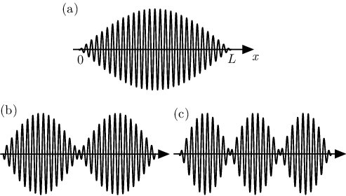
In the long wire limit, a good approximation for the excited mode is just

$$\Phi_{n}(x)=N\left(\begin{array}[]{c}-1\\ 1\end{array}\right)\sin(k_{F}x)\sin\left(\dfrac{\pi x}{L}\right)+\mathcal{O}(\ell^{-1})$$ (39)

with $N=\sqrt{2/L}$ the norm of the spinor. This is the one used in the main text, see $(\ref{eq:excited_states})$. Note that in the main text, we replace $\pi x/L\approx n\pi x/L=q$ such that the previous pure sine functions are valid only for long wires and for energies close to the gap. We numerically checked the difference between the approximate solution (3) and the exact ones (32) (with proper replacement $\Xi(\gamma)\mapsto X(\eta)$ of course) in term of the interaction matrix element (5) without finding discrepancy in the long wire limit $\ell\rightarrow\infty$.

More explicitly, one can show that the complete solutions $\Phi(x)$ for the excited states from Eq. (33) (after replacement of $\gamma\mapsto-i\eta$ of course) and the solution $\Phi_{0}(x)$ from Eq. (29) satisfies $\int_{0}^{L}dx\left[\Phi_{0}^{\dagger}(x)\Phi(x)\right]\approx e^{-\ell}$ whereas $\int_{0}^{L}dx\left[\Phi_{0}^{\dagger}(x)\tau^{z}\Phi(x)\right]\approx\ell^{-1/2}$ in the long wire limit. When calculating the overlap of the zero-energy mode and the excited ones, the exponential decay comes from the neglect in the expression of $\Phi_{0}(x)$ of the zero-energy mode situated at the right-end edge of the wire, this latter scaling as $e^{-\ell}$. The calculation can be done straightforwardly in the scale separation limit when $\sin^{2}(k_{F}x)\approx 1/2$, but this calculation has no specific interest to be written here, since the manipulation of the expression (33) is rather cumbersome. It nevertheless justifies the use of the interaction element (5) in the main text, in addition to the use of the approximate excited states (3).

Appendix B Evaluation of Eq. (19)

In this section, we give some details about the evaluation of Eq. (19). Especially, we comment the absence of specific propagating mode at a velocity well below the Fermi velocity.

We start by rewriting Eq. (19) in the form[50]

$$g(\omega,x,t)=\dfrac{2}{\pi\sqrt{\xi}}\int_{-t/2}^{t/2}d\tau\int_{0}^{\infty}d\eta\\ \times\left[e^{-i(\omega-\omega_{\Delta}\cosh\eta)\tau}\tanh\eta\sin\left(\dfrac{x}{\xi}\sinh\eta\right)\right].$$ (40)

Then we follow asymptotic methods evaluation of integrals.[51] We first evaluate the integral over $\eta$, defining

$$I(x<v_{F}\tau)=\int_{0}^{\infty}d\eta\tanh\eta\sin(\tilde{x}\sinh\eta)e^{i\tilde{\tau}\cosh\eta}\\ =\dfrac{1}{2i}\int_{-\infty}^{\infty}d\eta\tanh\eta e^{i\left(\tilde{\tau}\sqrt{1-\tilde{v}^{2}}\cosh\left(\arctanh\tilde{v}+\eta\right)\right)}$$ (41)

with $\tilde{x}=x/\xi$, $\tilde{\tau}=\omega_{\Delta}\tau$ and $\tilde{v}=\tilde{x}/\tilde{\tau}=x/v_{F}\tau$. The above expression is valid for $\tilde{v}<1$. One needs to use

$$I(x>v_{F}\tau)=\\ \dfrac{1}{2i}\int_{-\infty}^{\infty}d\eta\tanh\eta e^{i\left(\tilde{\tau}\sqrt{\tilde{v}^{2}-1}\sinh\left(\arctanh\tilde{v}^{-1}+\eta\right)\right)}$$ (42)

when $\tilde{v}>1$. These two limits are incompatible in the sense that $I\sim-\ln\sqrt{\tilde{x}^{2}-\tilde{\tau}^{2}}$ when $\tilde{v}\rightarrow 1$. So we have a first indication that (one of) the dominant contribution for the complete integral appears in the limit of Fermi velocity propagation $x\approx v_{F}t$.

For $v_{F}\tau\gg x$, one can deform the integral contour to $\eta=z-\arctanh\tilde{v}+i\arcsin(\tanh z)$ with $z$ the new integration variable. This path goes through the saddle-point at $\eta_{0}=i\sqrt{\tilde{\tau}^{2}-\tilde{x}^{2}}$. There is obviously no other complication in the $I(x,\tau)$ integral. Conventional evaluation then leads to

$$I(x\ll v_{F}\tau)\approx\sqrt{\dfrac{\pi}{2}}e^{3i\pi/4}e^{i\sqrt{\tilde{\tau}^{2}-\tilde{x}^{2}}}\dfrac{\tilde{x}}{\tilde{\tau}^{3/2}}$$ (43)

for this integral limit.

The second limit $v_{F}\tau\ll x$ has a stationary point at $\eta_{0}=-\arctanh\tilde{v}^{-1}+i\pi/2$ and its asymptotic

$$I(x\gg v_{F}\tau)\approx-\dfrac{\pi}{\sqrt{2}}e^{-\tilde{x}}+i\sqrt{\dfrac{\pi}{2}}e^{-\tilde{x}}\left(\dfrac{\tilde{\tau}}{\sqrt{\tilde{x}}}+\dfrac{\tilde{\tau}^{2}}{\tilde{x}}\right)$$ (44)

is easily obtained. For the moment we obtained a propagating wave-like behavior at velocity $v_{F}$ for large time $\tau$ and a Majorana localized wave-packet at position larger than $v_{F}\tau$. In other words, if an observer sits at the position $x$, the probability amplitude to find an extra quasi-particle is exponentially weak for times $\tau<x/v_{F}$ and has a power law decay on time for longer times.

To calculate the time integral, one uses that $\int_{-t/2}^{t/2}e^{i\omega\tau}d\tau=2\mathop{\rm Re}\left\{\int_{0}^{t/2}e^{i\omega\tau}d\tau\right\}$ such that one can convert $J(x,t)=\int_{-t/2}^{t/2}d\tau\left[e^{-i\omega\tau}I(x,\tau)\right]$ into an integral over positive $\tau$ only, since this is the only regime we calculated before. Note that $J=\pi\sqrt{\xi}g/2$ is just proportional to the $g(\omega,x,t)$ integral for which the above trick applies. The integral $J(x,t)=2\mathop{\rm Re}\left\{j(x,t)\right\}$ must be split in two parts $j(x,t)=j_{1}(x,t)+j_{2}(x,t)$ with

$$j_{1}(x,t) =\int_{0}^{x/v_{F}}I(x\gg v_{F}\tau)e^{-i\omega\tau}d\tau\propto e^{-x/\xi}$$ (45)

which disappears when one integrates $g^{2}$ for long wire, in the calculation of the $P_{\Gamma}(t)$. We will no more discuss this regime, which can be exactly calculated if required, but it is not relevant in the limit $\ell\gg 1$. The second contribution reads

$$j_{2}(x,t)=\int_{x/v_{F}}^{t/2}I(x\ll v_{F}\tau)e^{-i\omega\tau}d\tau$$ (46)

for the propagating wave-like integral. This latter integral can be evaluated by integration by part, since the dominant contributions arise at the boundaries. It gives

$$\omega_{\Delta}j_{2}\approx-\sqrt{\dfrac{\pi}{2}}e^{3i\pi/4}\tilde{x}\left[\dfrac{e^{-i\tilde{\omega}\tilde{x}}}{\tilde{x}^{5/2}}-\right.\\ \left.\dfrac{e^{i\sqrt{(\tilde{t}/2)^{2}-\tilde{x}^{2}}}e^{-i\tilde{\omega}\tilde{t}/2}}{(\tilde{t}/2)^{3/2}}\dfrac{i\sqrt{(\tilde{t}/2)^{2}-\tilde{x}^{2}}}{\tilde{\omega}\sqrt{(\tilde{t}/2)^{2}-\tilde{x}^{2}}-\tilde{t}/2}\right]$$ (47)

with $\tilde{t}=\omega_{\Delta}t$, $\tilde{x}=x/\xi$, and $\tilde{\omega}=\omega/\omega_{\Delta}$). The expression is valid when $x/v_{F}t\gg\sqrt{\omega^{2}-\omega_{\Delta}^{2}}/\omega=v_{g}/v_{F}$, i.e., when the Fermi velocity is larger than the effective group velocity $v_{g}$ associated to the noise spectrum density at frequency $\omega$. In the following we neglect the last contribution of $j_{2}$, since it is time independent. Eq. (47) leads to Eq. (21) of the main text, after taking twice the real part and neglecting the first line contribution, which is not time dependent.

In the opposite limit of a large effective group velocity, the integral $j_{2}$ has a saddle-point. To take into account this saddle-point obliged to consider the regime

$$\dfrac{(\tilde{\omega}^{2}-1)^{3/2}}{\tilde{t}}\ll\dfrac{\tilde{x}}{\tilde{t}}\ll\dfrac{\sqrt{\tilde{\omega}^{2}-1}}{\tilde{\omega}}$$ (48)

which in practice imposes the effective group velocity to be close to its maximum value $v_{g}\approx v_{F}$, since $\omega/\omega_{\Delta}$ is bounded to $1$ in order to make all the results valid, which means that there is no excitation frequencies below the gap. In that case, the integral equals

$$j_{2}(v_{g}\approx v_{F})\approx i\dfrac{\pi}{\sqrt{2}\omega_{\Delta}}\dfrac{e^{-i\tilde{x}\sqrt{\tilde{\omega}^{2}-1}}}{\tilde{\omega}^{3/2}\tilde{x}}$$ (49)

and thus correspond to an effective wave traveling at the effective group velocity $v_{g}$ only when $v_{g}\approx v_{F}$ in order for the condition (48) to be verified, so this regime never dominates in the final integral.

We carefully checked this point numerically as well. We never found a situation when the contribution $j_{2}(v_{g})$ is relevant, except when $v_{g}\approx v_{F}$, in which case the contribution (49) is well weaker than the dominant contribution (47) and can be safely discarded, as we do in the main text.

One still has to know the long time behavior of the full integral $g(\omega,x,t)$, when time is the largest parameter of the integral. This can be done by rewriting

$$g(\omega,x,t)=\dfrac{4}{\pi\omega_{\Delta}\sqrt{\xi}}\int_{1}^{\infty}dz\\ \times\dfrac{\sin\left(\tilde{x}\sqrt{z^{2}-1}\right)}{z}\dfrac{\sin\left(\tilde{t}\left(\tilde{\omega}-z\right)/2\right)}{\tilde{\omega}-z}$$ (50)

after the time integration is performed. When $\tilde{t}\rightarrow\infty$, the integral is peaked at $z=\tilde{\omega}$, so the first quotient can be ejected from the integral for the dominant contribution and the lower boundary can then be replaced by $-\infty$, and the remaining integral gives $\pi$. The latter argument is equivalent to saying that $\sin(\omega t)/\pi\omega$ behaves like a delta function $\delta(\omega)$ when $t\rightarrow\infty$. One obtains then

$$\lim_{\tau\rightarrow\infty}g(\omega,x,\tau)=\dfrac{4}{\omega\sqrt{\xi}}\sin\left(\tilde{x}\sqrt{\tilde{\omega}^{2}-1}\right)$$ (51)

for the leading term. The next correction term is obtained by an expansion at $z=1-i\epsilon$ for small $\epsilon$. It gives finally

$$g(x,\left(\omega-\omega_{\Delta})t\gg 1\right)\approx\dfrac{4}{\omega\sqrt{\xi}}\sin\left(\tilde{x}\sqrt{\tilde{\omega}^{2}-1}\right)\\ -\dfrac{8}{\omega_{\Delta}\sqrt{\pi\xi}}\dfrac{\tilde{x}}{\tilde{t}^{3/2}}\dfrac{\sin\left(\left(\tilde{\omega}-1\right)\dfrac{\tilde{t}}{2}+\dfrac{\pi}{4}\right)}{\tilde{\omega}-1}$$ (52)

for large time. Thus the integral goes to a finite value at infinite time, oscillating in space with a small wave-vector $\sqrt{\omega^{2}-\omega_{\Delta}^{2}}/v_{F}$ when the noise frequency approaches the gap frequency. On top of these spatial oscillations, there is some wiggling time behavior with long waves, too. Eq. (52) leads to Eq. (20) in the main text.

It is pretty difficult to compare our asymptotic expansions at each step of the calculation, since all the integrals are difficult to integrate even numerically. Nevertheless, to compare our asymptotic results with the exact integral $J(x,t)$, we neglect the $j_{1}$ contribution as it is exponentially small; i.e., we compare (twice the real part of) Eq. (47) in the short time limit and Eq. (52) valid for long time with the numerical evaluation of the complete integral Eq. (19). Some characteristic curves are given in Fig. 4.

References

- [1] A. Yu. Kitaev, Phys. Usp. 44 (suppl.), 131 (2001).
- [2] S. Das Sarma, M. Freedman, and C. Nayak, Phys. Rev. Lett. 94, 166802 (2005).
- [3] C. Nayak, A. Stern, M. Freedman, and S. Das Sarma, Rev. Mod. Phys. 80, 1083 (2008).
- [4] J. Alicea, Y. Oreg, G. Refael, F. von Oppen, and M. P. A. Fisher, Nat. Phys. 7, 412 (2011).
- [5] J. D. Sau, D. J. Clarke, and S. Tewari, Phys. Rev. B 84, 094505 (2011).
- [6] B. van Heck, A. R. Akhmerov, F. Hassler, M. Burrello, and C. W. J. Beenakker, New J. Phys. 14, 035019 (2011).
- [7] C. W. J. Beenakker, Annu. Rev. Con. Mat. Phys. 4, 113 (2013).
- [8] J. Alicea, Rep. Prog. Phys. 75, 076501 (2012).
- [9] M. Leijnse and K. Flensberg, Phys. Rev. B 84, 140501(R) (2011).
- [10] J. C. Budich, S. Walter, and B. Trauzettel, Phys. Rev. B 85, 121405(R) (2012).
- [11] R. M. Lutchyn, J. D. Sau, and S. Das Sarma, Phys. Rev. Lett. 105, 077001 (2010).
- [12] Y. Oreg, G. Refael, and F. von Oppen, Phys. Rev. Lett. 105, 177002 (2010).
- [13] J. D. Sau, S. Tewari, R. M. Lutchyn, T. Stanescu, S. Das Sarma, Phys. Rev. B 82, 214509 (2010).
- [14] V. Mourik, K. Zuo, S. M. Frolov, S. R. Plissard, E. P. A. M. Bakkers, and L. P. Kouwenhoven, Science 336, 1003 (2012).
- [15] M. T. Deng, C. L. Yu, G. Y. Huang, M. Larsson, P. Caroff, and H. Q. Xu, arXiv:1204.4130 (2012).
- [16] A. Das, Y. Ronen, Y. Most, Y. Oreg, M. Heiblum, and H. Shtrikman, Nat. Phys. 8, 887 (2012).
- [17] A. D. K. Finck, D. J. V. Harlingen, P. K. Mohseni, K. Jung, and X. Li, Phys. Rev. Lett. 110, 126406 (2013).
- [18] H. O. H. Churchill, V. Fatemi, K. Grove-Rasmussen, M. T. Deng, P. Caroff, H. Q. Xu, and C. M. Marcus, arXiv:1303.2407 (2013).
- [19] M. Franz, Nature Nanotechnology 8, 149 (2013).
- [20] G. Goldstein and C. Chamon, Phys. Rev. B 84, 205109 (2011).
- [21] M. J. Schmidt, D. Rainis, and D. Loss, Phys. Rev. B 86, 085414 (2012).
- [22] E. Dennis, A. Kitaev, A. Landahl, and J. Preskill, J. Math. Phys. 43, 4452 (2002).
- [23] A. R. Akhmerov, Phys. Rev. B 82, 020509 (2010).
- [24] J. D. Sau, R. M. Lutchyn, S. Das Sarma, and S. Tewari, Phys. Rev. Lett. 104, 040502 (2010).
- [25] G. E. Volovik, Universe in a Helium Droplet (Oxford University Press, 2003).
- [26] L. Gor’kov and E. Rashba, Phys. Rev. Lett. 87, 37004 (2001).
- [27] J. D. Sau, R. M. Lutchyn, S. Tewari, and S. Das Sarma, Phys. Rev. Lett. 104, 040502 (2010).
- [28] J. Alicea, Phys. Rev. B 81, 125318 (2010).
- [29] K. Sengupta, I. Žutić, H.-J. Kwon, V. M. Yakovenko, and S. Das Sarma, Phys. Rev. B 63, 144531 (2000).
- [30] J. Klinovaja and D. Loss, Phys. Rev. B 86, 085408 (2012).
- [31] M. Tinkham, Introduction to superconductivity, (McGraw-Hill, New York, 1996).
- [32] R. J. Schoelkopf, A. A. Clerk, S. M. Girvin, K. W. Lehnert, and M. H. Devoret, in Quantum Noise in Mesoscopic Physics, edited by Yu. V. Nazarov (Kluwer Academic, Dordrecht, 2003).
- [33] The previous argument is equivalent to saying that behaves like when .
- [34] Ya. M. Blanter and M. Büttiker, Phys. Rep. 336, 1 (2000), section 3.2.1.
- [35] G. Catelani, S. E. Nigg, S. M. Girvin, R. J. Schoelkopf, and L. I. Glazman, Phys. Rev. B 86, 184514 (2012).
- [36] C. Cohen-Tannoudji, J. Dupont-Roc, and G. Grynberg, Atom-Photon Interactions (Wiley, New York, 1992), chapter .
- [37] F. Hassler, A. Rüegg, M. Sigrist, and G. Blatter, Phys. Rev. Lett. 104, 220402 (2010).
- [38] The static contribution vanishes exponentially in the space-integration over the half-wire and is thus neglected from the beginning.
- [39] C. Stark, L. Pollet, A. Imamoǧlu, and R. Renner, Phys. Rev. Lett. 107, 030504 (2011).
- [40] J. R. Wootton and J. K. Pachos, Phys. Rev. Lett. 107, 030503 (2011).
- [41] S. Bravyi and R. König, Comm. Math. Phys. 316, 641 (2012).
- [42] K. H. Bennemann and J. B. Ketterson, Superconductivity (Springer, Berlin, 2008).
- [43] P. W. Brouwer, M. Duckheim, A. Romito, and F. von Oppen, Phys. Rev. B 84, 144526 (2011).
- [44] S. Tewari, T. D. Stanescu, J. D. Sau, S. Das Sarma, Phys. Rev. B 86, 024504 (2012).
- [45] V. Kogan, Phys. Rev. B 31, 1318 (1985).
- [46] P. Neven, D. Bagrets, and A. Altland, New J. Phys. 15, 055019 (2013).
- [47] V. P. Mineev and K. Samokhin, Introduction to unconventionnal superconductivity (Gordon and Breach Science Publishers, 1998).
- [48] S. Ryu, A. P. Schnyder, A. Furusaki, and A. W. W. Ludwig, New J. Phys. 12, 065010 (2010).
- [49] I. Fulga, F. Hassler, and A. R. Akhmerov, Phys. Rev. B 85, 165409 (2012).
- [50] We use the completeness relation , the definitions and for the quasi-particle modes; also, as is large.
- [51] C. M. Bender and S. A. Orszag, Advanced Mathematical Methods for Scientists and Engineers: Asymptotic Methods and Perturbation Theory (Springer, New York, 1978).