Metric-Free Natural Gradient for Joint-Training of Boltzmann Machines

Abstract

This paper introduces the Metric-Free Natural Gradient (MFNG) algorithm for training Boltzmann Machines. Similar in spirit to the Hessian-Free method of Martens 2010, our algorithm belongs to the family of truncated Newton methods and exploits an efficient matrix-vector product to avoid explicitly storing the natural gradient metric $L$. This metric is shown to be the expected second derivative of the log-partition function (under the model distribution), or equivalently, the covariance of the vector of partial derivatives of the energy function. We evaluate our method on the task of joint-training a 3-layer Deep Boltzmann Machine and show that MFNG does indeed have faster per-epoch convergence compared to Stochastic Maximum Likelihood with centering, though wall-clock performance is currently not competitive.

1 Introduction

Boltzmann Machines (BM) have become a popular method in Deep Learning for performing feature extraction and probability modeling. The emergence of these models as practical learning algorithms stems from the development of efficient training algorithms, which estimate the negative log-likelihood gradient by either contrastive [4] or stochastic [18, 19] approximations. However, the success of these models has for the most part been limited to the Restricted Boltzmann Machine (RBM) [6], whose architecture allows for efficient exact inference. Unfortunately, this comes at the cost of the model’s representational capacity, which is limited to a single layer of latent variables. The Deep Boltzmann Machine (DBM) [15] addresses this by defining a joint energy function over multiple disjoint layers of latent variables, where interactions within a layer are prohibited. While this affords the model a rich inference scheme incorporating top-down feedback, it also makes training much more difficult, requiring until recently an initial greedy layer-wise pretraining scheme. Since, Montavon and Muller 2012 have shown that this difficulty stems from an ill-conditioning of the Hessian matrix, which can be addressed by a simple reparameterization of the DBM energy function, a trick called centering (an analogue to centering and skip-connections found in the deterministic neural network literature [17, 14]). As the barrier to joint-training is overcoming a challenging optimization problem, it is apparent that second-order gradient methods might prove to be more effective than simple stochastic gradient methods. This should prove especially important as we consider models with increasingly complex posteriors or higher-order interactions between latent variables.

To this end, we explore the use of the Natural Gradient [2], which seems ideally suited to the stochastic nature of Boltzmann Machines. Our paper is structured as follows. Section 2 provides a detailed derivation of the natural gradient, including its specific form for BMs. While most of these equations have previously appeared in [3], our derivation aims to be more accessible as it attempts to derive the natural gradient from basic principles, while minimizing references to Information Geometry. Section 3 represents the true contribution of the paper: a practical natural gradient algorithm for BMs which exploits the persistent Markov chains of Stochastic Maximum Likelihood (SML) [18], with a Hessian-Free (HF) like algorithm [8]. The method, named Metric-Free Natural Gradient (MFNG) (in recognition of the similarities of our method to HF), avoids explicitly storing the natural gradient metric $L$ and uses a linear solver to perform the required matrix-vector product $L^{-1}\mathbb{E}_{q}\left[\nabla\log p_{\theta}\right]$. Preliminary experimental results on DBMs are presented in Section 4, with the discussion appearing in Section 5.

2 The Natural Gradient

2.1 Motivation and Derivation

The main insight behind the natural gradient is that the space of all probability distributions $\mathcal{P}=\{p_{\theta}(x);\ \theta\in\Theta,x\in\chi\}$ forms a Riemannian manifold. Learning, which typically proceeds by iteratively adapting the parameters $\theta$ to fit an empirical distribution $q$, thus traces out a path along this manifold. An immediate consequence is that following the direction of steepest descent in the original Euclidean parameter space does not correspond to the direction of steepest descent along $\mathcal{P}$. To do so, one needs to account for the metric describing the local geometry of the manifold, which is given by the Fisher Information matrix [1], shown in Equation 4. While this metric is typically derived from Information Geometry, a derivation more accessible to a machine learning audience can be obtained as follows.

The natural gradient aims to find the search direction $\Delta\theta$ which minimizes a given objective function, such that the Kullback–Leibler divergence $KL(p_{\theta}\parallel p_{\theta+\Delta\theta})$ remains constant throughout optimization. This constraint ensures that we make constant progress regardless of the curvature of the manifold $\mathcal{P}$ and enforces an invariance to the parameterization of the model. The natural gradient for maximum likelihood can thus be formalized as:

$$\nabla_{N}:=\Delta\theta^{*} \leftarrow \text{argmin}_{\Delta\theta}\ \mathbb{E}_{q}\left[-\log p_{\theta+\Delta\theta}(x)\right]$$ (1)

s.t. $$KL(p_{\theta}\parallel p_{\theta+\Delta\theta})=\mathrm{const.}$$

In order to derive a useful parameter update rule, we will consider the KL divergence under the assumption $\Delta\theta\rightarrow 0$. We also assume we have a discrete and bounded domain $\chi$ over which we define the probability mass function $p_{\theta}$. Taking the Taylor series expansion of $\log p_{\theta+\Delta\theta}$ around $\theta$, and denoting $\nabla f$ as the column vector of partial derivatives with $\frac{\partial f}{\partial\theta_{i}}$ as the $i$-th entry, and $\nabla^{2}f$ the Hessian matrix with $\frac{\partial^{2}f}{\partial\theta_{i}\partial\theta_{j}}$ in position $(i,j)$, we have:

$$KL(p_{\theta}\parallel p_{\theta+\Delta\theta}) \approx \sum_{\chi}p_{\theta}\log p_{\theta}-\sum_{\chi}p_{\theta}\left[\log p_{\theta}+\left(\nabla\log p_{\theta}\right)^{T}\Delta\theta+\frac{1}{2}\Delta\theta^{T}\left(\nabla^{2}\log p_{\theta}\right)\Delta\theta\right]$$ (2)

$$= \frac{1}{2}\Delta\theta^{T}\mathbb{E}_{p_{\theta}}\left[-\nabla^{2}\log p_{\theta}\right]\Delta\theta$$

with the transition stemming from the fact that $\sum_{\chi}p_{\theta}\frac{\partial\log p_{\theta}}{\partial\theta_{i}}=\frac{\partial}{\partial\theta_{i}}\sum_{x\in\chi}p_{\theta}(x)=0$. Replacing the objective function of Equation 1 by its first-order Taylor expansion and rewriting the constraint as a Lagrangian, we arrive at the following formulation for $\mathcal{L}(\theta,\Delta\theta)$, the loss function which the natural gradient seeks to minimize.

$$\mathcal{L}(\theta,\Delta\theta) = \mathbb{E}_{q}\left[-\log p_{\theta}\right]+\mathbb{E}_{q}\left[-\nabla\log p_{\theta}\right]^{T}\Delta\theta+\frac{\lambda}{2}\Delta\theta^{T}\mathbb{E}_{p_{\theta}}\left[-\nabla^{2}\log p_{\theta}\right]\Delta\theta.$$

Setting $\frac{\partial\mathcal{L}}{\partial\Delta\theta}$ to zero yields the natural gradient direction $\nabla_{N}$:

$$\nabla_{N}=L^{-1}\mathbb{E}_{q}\left[\nabla\log p_{\theta}\right]\text{ with }L = \mathbb{E}_{p_{\theta}}\left[-\nabla^{2}\log p_{\theta}\right]$$ (3)

$$\text{ or equivalently }L = \mathbb{E}_{p_{\theta}}\left[\nabla\log p_{\theta}\nabla^{T}\log p_{\theta}\right]$$ (4)

While its form is reminiscent of the Newton direction, the natural gradient multiplies the estimated gradient by the inverse of the expected Hessian of $\log p_{\theta}$ (Equation 3) or equivalently by the Fisher Information matrix (FIM, Equation 4). The equivalence between both expressions can be shown trivially, with the details appearing in the Appendix. We stress that both of these expectations are computed with respect to the model distribution, and thus computing the metric $L$ does not involve the empirical distribution in any way. The FIM for Boltzmann Machines is thus not equal to the uncentered covariance of the maximum likelihood gradients. In the following, we pursue our derivation from the form given in Equation 4.

2.2 Natural Gradient for Boltzmann Machines

Derivation.

Boltzmann machines define a joint distribution over a vector of binary random variables $x\in\{0,1\}^{N}$ by way of an energy function $E(x)=-\sum_{k<l}W_{kl}x_{k}x_{l}-\sum_{k}b_{k}x_{k}$, with weight matrix $W\in\mathbb{R}^{N\times N}$ and bias vector $b\in\mathbb{R}^{N}$. Energy and probability are related by the Boltzmann distribution, such that $p(x)=\frac{1}{Z}\exp\left(-E(x)\right)$, with $Z$ the partition function defined by $Z=\sum_{x}\exp\left(-E(x)\right)$.

Starting from the expression of $L$ found in Equation 3, we can derive the natural gradient metric for Boltzmann Machines.

$$L^{(BM)} = \mathbb{E}_{p_{\theta}}\left[\nabla^{2}E(x)+\nabla^{2}\log Z\right]=\mathbb{E}_{p_{\theta}}\left[\nabla^{2}\log Z\right]$$

The natural gradient metric for first-order BMs takes on a surprisingly simple form: it is the expected Hessian of the log-partition function. With a few lines of algebra (whose details are presented in the Appendix), we can rewrite it as follows:

$$L^{(BM)} = \mathbb{E}_{p_{\theta}}\left[\left(\nabla E(x)-\mathbb{E}_{p_{\theta}}\left[\nabla E(x)\right]\right)^{T}\left(\nabla E(x)-\mathbb{E}_{p_{\theta}}\left[\nabla E(x)\right]\right)\right]$$ (5)

$L^{(BM)}$ is thus given by the covariance of $\nabla E$, measured under the model distribution $p_{\theta}$. Concretely, if we denote $W_{kl}$ and $W_{mn}$ as the i and j-th parameters of the model respectively, the entry $L_{ij}$ will take on the value $-\mathbb{E}\left[x_{k}x_{l}x_{m}x_{n}\right]+\mathbb{E}\left[x_{k}x_{l}\right]\mathbb{E}\left[x_{m}x_{n}\right]$.

Discussion.

When computing the Taylor expansion of the KL divergence in Equation 2, we glossed over an important detail. Namely, how to handle latent variables in $p_{\theta}(x)$, a topic first discussed in [3]. If $x=[v,h]$, we could just as easily have derived the natural gradient by considering the constraint $KL\left(\sum_{h}p_{\theta}(v,h)\parallel\sum_{h}p_{\theta+\Delta\theta}(v,h)\right)=\text{const}$. Alternatively, since the distinction between visible and hidden units is entirely artificial (since the KL divergence does not involve the empirical distribution), we may simply wish to consider the distribution obtained by analytically integrating out a maximal number of random variables. In a DBM, this would entail marginalizing over all odd or even layers, a strategy employed with great success in the context of AIS [15]. In this work however, we only consider the metric obtained by considering the $KL$ divergence between the full joint distributions $p_{\theta}$ and $p_{\theta+\Delta\theta}$.

3 Metric-Free Natural Gradient Implementation

We can compute the natural gradient $\nabla_{N}$ by first replacing the expectations of Equation 5 by a finite sample approximation. We can do this efficiently by reusing the model samples generated by the persistent Markov chains of SML. Given the size of the matrix being estimated however, we expect this method to require a larger number of chains than is typically used. The rest of the method is similar to the Hessian-Free (HF) algorithm of Martens 2010: we exploit an efficient matrix-vector implementation combined with a linear-solver, such as Conjugate Gradient or MinRes[12], to solve the system $Ly=\mathbb{E}_{q}\left[\nabla\log p_{\theta}\right]$ for $y\in\mathbb{R}^{N}$. Additionally, we replace the expectation on the rhs. of this previous equation by an average computed over a mini-batch of training examples (sampled from the empirical distribution $q$), as is typically done in the stochastic learning setting.

For Boltzmann Machines, the matrix-vector product $Ly$ can be computed in a straightforward manner, without recourse to Pearlmutter’s R-operator [13]. Starting from a sampling approximation to Equation 5, we simply push the dot product inside of the expectation as follows:

$$L^{(BM)}y \approx \left(S-\bar{S}\right)^{T}\left[\left(S-\bar{S}\right)y\right]$$ (6)

with $$S\in\mathbb{R}^{M\times N}\text{, the matrix with entries }s_{mj}=\frac{\partial E(x_{m})}{\partial\theta_{j}}$$

and $$\bar{S}\in\mathbb{R}^{N}\text{, the vector with entries }s_{j}=\frac{1}{M}\sum_{m}s_{mj}$$

and $$x_{m}\sim p_{\theta}(x),m\in[1,M].$$

By first computing the matrix-vector product $(S-\bar{S})y$, we can easily avoid computing the full $N\times N$ matrix $L$. Indeed, the result of this operation is a vector of length $M$, which is then left-multiplied by a matrix of dimension $N\times M$, yielding the matrix-vector product $Ly\in\mathbb{R}^{N}$. A single iteration of the MFNG is presented in Algorithm 1. A full open-source implementation is also available online..

Algorithm 1 ${\tt MFNG\_iteration}(\theta,\mathcal{X^{+}},\mathcal{Z}^{-}_{old})$
$\theta$: parameters of the model. $N\vcentcolon=\mid\theta\mid$.
$\mathcal{X}^{+}$: mini-batch of training examples, with $\mathcal{X}^{+}=\{x_{m};m\in[1,M]\}$.
$\mathcal{Z}_{old}^{-}$: previous state of Markov chains, with $\mathcal{Z}=\{z_{m}\vcentcolon=(v_{m},h^{(1)}_{m},h^{(2)}_{m});m\in[1,M]\}$

 $\bullet$ Generate positive phase samples $\mathcal{Z}^{+}=\{z^{+}_{m}\vcentcolon=(x_{m},h^{(1)+}_{m},h^{(2)+}_{m});m\in[1,M]\}$

 $\bullet$ Initializing $M$ Markov chains from state $\mathcal{Z}^{-}_{old}$, generate negative phase samples $\mathcal{Z}^{-}_{new}$.

 $\bullet$ Compute the vectors $s^{+}_{m}=\frac{\partial E(z^{+}_{m})}{\partial\theta}$ and $s^{-}_{m}=\frac{\partial E(z^{-}_{m})}{\partial\theta}$, $\forall m$.

 $\bullet$ Compute negative log-likelihood gradient as $g=\frac{1}{M}\sum_{m}\left(s^{+}_{m}-s^{-}_{m}\right)$.

 $\bullet$ Denote $S\in\mathbb{R}^{M\times N}$ as the matrix with rows $s^{-}_{m}$ and $\bar{S}=\frac{1}{M}\sum_{m}s^{-}_{m}$.

 # Solve the system “$Ly=g$” for y, given $L=(S-\bar{S})^{T}(S-\bar{S})$ and an initial zero vector.

 # computeLy is a function which performs equation  6, without instantiating $L$.

 $\bullet$ $\nabla_{N}\theta\leftarrow{\tt CGSolve}({\tt computeLy},S,g,{\tt zeros}(N))$

4 Experiments

We performed a proof-of-concept experiment to determine whether our Metric-Free Natural Gradient (MFNG) algorithm is suitable for joint-training of complex Boltzmann Machines. To this end, we compared our method to Stochastic Maximum Likelihood and a diagonal approximation of MFNG on a 3-layer Deep Boltzmann Machine trained on MNIST [7]. All algorithms were run in conjunction with the centering strategy of Montavon and Muller 2012, which proved crucial to successfully joint-train all layers of the DBM (even when using MFNG) . We chose a small 3-layer DBM with 784-400-100 units at the first, second and third layers respectively, to be comparable to [10]. Hyper-parameters were varied as follows. For inference, we ran $5$ iterations of either mean-field as implemented in [15] or Gibbs sampling. The learning rate was kept fixed during training and chosen from the set $\{5\cdot 10^{-3},10^{-3},10^{-4}\}$. For MinRes, we set the damping coefficient to $0.1$ and used a fixed tolerance of $10^{-5}$ (used to determine convergence). Finally, we tested all algorithms on minibatch sizes of either $25$, $128$ or $256$ elements . Finally, since we are comparing optimization algorithms, hyper-parameters were chosen based on the training set likelihood (though we still report the associated test errors). All experiments used the MinRes linear solver, both for its speed and its ability to return pseudo-inverses when faced with ill-conditioning.

Figure 1 (left) shows the likelihood as estimated by Annealed Importance Sampling [15, 11] as a function of the number of epochs . Under this metric, MFNG achieves the fastest convergence, obtaining a training/test set likelihood of $-71.26$/$-72.84$ nats after 94 epochs. In comparison, MFNG-diag obtains $-73.22$/$-74.05$ nats and SML $-80.12$/$-79.71$ nats in 100 epochs. The picture changes however when plotting likelihood as a function of CPU-time, as shown in Figure 1 (right). Given a wall-time of $8000$s for MFNG and SML, and $5000$s for MFNG-diag, SML is able to perform upwards of $1550$ epochs, resulting in an impressive likelihood score of $-64.94$ / $-67.73$. Note that these results were obtained on the binary-version of MNIST (thresholded at 0.5) in order to compare to [10]. These results are therefore not directly comparable to [15], which binarizes the dataset through sampling (by treating each pixel activation as the probability $p$ of a Bernouilli distribution).

Figure 1: Estimated model likelihood as a function of (left) epochs and (right) CPU-time for MFNG, its diagonal approximation (MFNG-diag) and SML. All methods were run in conjunction with the DBM centering trick [9], with centering coefficients held fixed during training. Our grid search yielded the following hyper-parameters: batch size of $256/128$ for MFNG(-diag)/SGD; 5 steps of mean-field / sampling-based inference for MFNG(-diag)/SGD and a learning rate of $5\cdot 10^{-3}$.

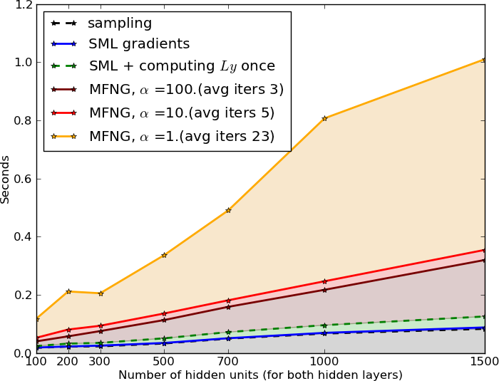
Figure 2 shows a breakdown of the algorithm runtime, for various components of the algorithm. These statistics were collected in the early stages of training, but are generally representative of the bigger picture. While the linear solver clearly dominates the runtime, there are a few interesting observations to make. For small models and batch sizes greater than $256$, a single evaluation of $Ly$ appears to be of the same order of magnitude as a gradient evaluation. In all cases, this cost is smaller than that of sampling, which represents a non-negligible part of the total computational budget. This suggests that MFNG could become especially attractive for models which are expensive to sample from. Overall however, restricting the number of CG/MinRes iterations appears key to computational performance, which can be achieved by increasing the damping factor $\alpha$. How this affects convergence in terms of likelihood is left for future work.

Figure 2: Breakdown of algorithm runtime, when we vary (left) the batch size (with fixed model architecture $784-400-100$) and (right) the model size (with fixed batch size of $256$). Runtime is additive in the order given by the labels (top to bottom). Dotted lines denote intermediate steps, while continuous lines denote full steps. Data was collected on a Nvidia GTX 480 card.

5 Discussion and Future Work

While the wall-clock performance of MFNG is not currently competitive with SML, we believe there are still many avenues to explore to improve computational efficiency. Firstly, we performed almost no optimization of the various MinRes hyper-parameters. In particular, we ran the algorithm to convergence with a fixed tolerance of $10^{-5}$. While this typically resulted in relatively few iterations (around $15$), this level of precision might not be required (especially given the stochastic nature of the algorithm). Additionally, it could be worth exploiting the same strategy as HF where the linear solver is initialized by the solution found in the previous iteration. This may prove much more efficient than the current approach of initializing the solver with a zero vector. Pre-conditioning is also a well-known method for accelerating the convergence speed of linear solvers [5]. Our implementation used a simple diagonal regularization of $L$. The Jacobi preconditioner could be implemented easily however by computing the diagonal of $L$ in a first-pass.

Finally, while our single experiment offers little evidence in support of either conclusion, it may very well be possible that MFNG is simply not computationally efficient for DBMs, compared to SML with centering. In this case, it would be worth applying the method to either (i) models with known ill-conditioning, such as factored 3-rd order Boltzmann Machines or (ii) models and distributions exhibiting complex posterior distributions. In such scenarios, we may wish to maximize the use of the positive phase statistics (which were obtained at a high computational cost) by performing larger jumps in parameter space. It remains to be seen how this would interact with SML, where the burn-in period of the persistent chains is directly tied to the magnitude of $\Delta\theta$.

Appendix

We include the following derivations for completeness.

5.1 Expected Hessian of $\log Z$ and Fisher Information.

$$\mathbb{E}_{p_{\theta}}\left[-\frac{\partial^{2}\log p(x)}{\partial\theta_{i}\partial\theta_{j}}\right] = \mathbb{E}_{p_{\theta}}\left[\frac{1}{p(x)^{2}}\frac{\partial p(x)}{\partial\theta_{j}}\frac{\partial p(x)}{\partial\theta_{i}}-\frac{1}{p(x)}\frac{\partial^{2}p(x)}{\partial\theta_{i}\partial\theta_{j}}\right]$$

$$= \mathbb{E}_{p_{\theta}}\left[\left(\frac{1}{p(x)}\frac{\partial p(x)}{\partial\theta_{i}}\right)\left(\frac{1}{p(x)}\frac{\partial p(x)}{\partial\theta_{j}}\right)-\frac{1}{p(x)}\frac{\partial^{2}p(x)}{\partial\theta_{i}\partial\theta_{j}}\right]$$

$$= \mathbb{E}_{p_{\theta}}\left[\frac{\partial\log p(x)}{\partial\theta_{i}}\frac{\partial\log p(x)}{\partial\theta_{j}}\right]-\sum_{x}p(x)\frac{1}{p(x)}\frac{\partial^{2}p(x)}{\partial\theta_{i}\partial\theta_{j}}$$

$$= \mathbb{E}_{p_{\theta}}\left[\frac{\partial\log p(x)}{\partial\theta_{i}}\frac{\partial\log p(x)}{\partial\theta_{j}}\right]-\sum_{x}\frac{\partial^{2}p(x)}{\partial\theta_{i}\partial\theta_{j}}$$

$$= \mathbb{E}_{p_{\theta}}\left[\frac{\partial\log p(x)}{\partial\theta_{i}}\frac{\partial\log p(x)}{\partial\theta_{j}}\right]-\frac{\partial^{2}\sum_{x}p(x)}{\partial\theta_{i}\partial\theta_{j}}$$

$$= \mathbb{E}_{p_{\theta}}\left[\frac{\partial\log p(x)}{\partial\theta_{i}}\frac{\partial\log p(x)}{\partial\theta_{j}}\right]$$

5.2 Derivation of Equation 5

$$\log p(x) = -E(x)-\log Z$$

$$\frac{\partial\log p(x)}{\partial\theta_{i}} = -\frac{\partial E(x)}{\partial\theta_{i}}-\frac{1}{Z}\sum_{x}\frac{\partial}{\partial\theta_{i}}\left[\exp\left(-E(x)\right)\right]$$

$$= -\frac{\partial E(x)}{\partial\theta_{i}}+\mathbb{E}_{p_{\theta}}\left[\frac{\partial E(x)}{\partial\theta_{i}}\right]$$

$$\mathbb{E_{p_{\theta}}}\left[-\frac{\partial^{2}\log p(x)}{\partial\theta_{i}\partial\theta_{j}}\right] = \mathbb{E}_{p_{\theta}}\left[\left(\frac{\partial E(x)}{\partial\theta_{i}}-\mathbb{E}_{p_{\theta}}\left[\frac{\partial E(x)}{\partial\theta_{i}}\right]\right)\left(\frac{\partial E(x)}{\partial\theta_{j}}-\mathbb{E}_{p_{\theta}}\left[\frac{\partial E(x)}{\partial\theta_{j}}\right]\right)\right]$$

$$= \mathbb{E}_{p_{\theta}}\left[\frac{\partial E(x)}{\partial\theta_{i}}\frac{\partial E(x)}{\partial\theta_{j}}\right]-\mathbb{E}_{p_{\theta}}\left[\frac{\partial E(x)}{\partial\theta_{i}}\right]\mathbb{E}_{p_{\theta}}\left[\frac{\partial E(x)}{\partial\theta_{j}}\right]$$

References

- Amari [1985] Amari, S. (1985). Differential geometrical methods in statistics. Lecture notes in statistics, 28.
- Amari [1998] Amari, S. (1998). Natural gradient works efficiently in learning. Neural Computation, 10(2), 251–276.
- Amari et al. [1992] Amari, S., Kurata, K., and Nagaoka, H. (1992). Information geometry of Boltzmann machines. IEEE Trans. on Neural Networks, 3, 260–271.
- Carreira-Perpiñan and Hinton [2005] Carreira-Perpiñan, M. A. and Hinton, G. E. (2005). On contrastive divergence learning. In AISTATS’2005, pages 33–40.
- Chapelle and Erhan [2011] Chapelle, O. and Erhan, D. (2011). Improved preconditioner for hessian free optimization. NIPS Workshop on Deep Learning and Unsupervised Feature Learning.
- Freund and Haussler [1992] Freund, Y. and Haussler, D. (1992). A fast and exact learning rule for a restricted class of Boltzmann machines. pages 912–919, Denver, CO. Morgan Kaufmann, San Mateo.
- LeCun et al. [1998] LeCun, Y., Bottou, L., Bengio, Y., and Haffner, P. (1998). Gradient based learning applied to document recognition. Proc. IEEE.
- Martens [2010] Martens, J. (2010). Deep learning via Hessian-free optimization. pages 735–742.
- Montavon and Muller [2012] Montavon, G. and Muller, K.-R. (2012). Deep Boltzmann machines and the centering trick. In G. Montavon, G. Orr, and K.-R. Muller, editors, Neural Networks: Tricks of the Trade, volume 7700 of Lecture Notes in Computer Science, pages 621–637.
- Montavon and Müller [2012] Montavon, G. and Müller, K.-R. (2012). Learning feature hierarchies with centered deep Boltzmann machines. CoRR, abs/1203.4416.
- Neal [2001] Neal, R. M. (2001). Annealed importance sampling. Statistics and Computing, 11(2), 125–139.
- Paige and Saunders [1975] Paige, C. C. and Saunders, M. A. (1975). Solution of Sparse Indefinite Systems of Linear Equations. SIAM Journal on Numerical Analysis, 12(4), 617–629.
- Pearlmutter [1994] Pearlmutter, B. (1994). Fast exact multiplication by the Hessian. Neural Computation, 6(1), 147–160.
- Raiko et al. [2012] Raiko, T., Valpola, H., and LeCun, Y. (2012). Deep learning made easier by linear transformations in perceptrons. In AISTATS’2012.
- Salakhutdinov and Hinton [2009] Salakhutdinov, R. and Hinton, G. (2009). Deep Boltzmann machines. In Proceedings of the Twelfth International Conference on Artificial Intelligence and Statistics (AISTATS 2009), volume 8.
- Salakhutdinov and Murray [2008] Salakhutdinov, R. and Murray, I. (2008). On the quantitative analysis of deep belief networks. volume 25, pages 872–879.
- Schraudolph [1998] Schraudolph, N. N. (1998). Centering neural network gradient factors. In G. B. Orr and K.-R. Muller, editors, Neural Networks: Tricks of he Trade, pages 548–548. Springer.
- Tieleman [2008] Tieleman, T. (2008). Training restricted Boltzmann machines using approximations to the likelihood gradient. pages 1064–1071.
- Younes [1999] Younes, L. (1999). On the convergence of Markovian stochastic algorithms with rapidly decreasing ergodicity rates. Stochastics and Stochastic Reports, 65(3), 177–228.