Graph-based Code Design for Quadratic-Gaussian Wyner-Ziv Problem with Arbitrary Side Information

Abstract

Wyner-Ziv coding (WZC) is a compression technique using decoder side information, which is unknown at the encoder, to help the reconstruction. In this paper, we propose and implement a new WZC structure, called residual WZC, for the quadratic-Gaussian Wyner-Ziv problem where side information can be arbitrarily distributed. In our two-stage residual WZC, the source is quantized twice and the input of the second stage is the quantization error (residue) of the first stage. The codebook of the first stage quantizer must be simultaneously good for source and channel coding, since it also acts as a channel code at the decoder. Stemming from the non-ideal quantization at the encoder, a problem of channel decoding beyond capacity is identified and solved when we design the practical decoder. Moreover, by using the modified reinforced belief-propagation quantization algorithm, the low-density parity check code (LDPC), whose edge degree is optimized for channel coding, also performs well as a source code. We then implement the residual WZC by an LDPC and a low-density generator matrix code (LDGM). The simulation results show that our practical construction approaches the Wyner-Ziv bound. Compared with previous works, our construction can offer more design flexibility in terms of distribution of side information and practical code rate selection.

I Introduction

Wyner-Ziv coding (WZC) [1], which is a generalization of the lossless Slepian-Wolf coding (SWC) [2], refers to a lossy source coding with side information at the decoder only. Among the applications of WZC [3], one important scenario is the quadratic-Gaussian problem, where the difference between the source and the side information is Gaussian and mean-square error (MSE) is adopted as the distortion measure. For this case, WZC does not incur rate loss when compared with source coding with side information available at both the encoder and the decoder. This zero-rate-loss result was originally proved for the case where the side information is Gaussian [1], but recently generalized to the case where the side information can be arbitrarily distributed [4]. There are many applications of quadratic-Gaussian WZC, such as distributed source coding in the sensor networks [3] and the protocols in the relay networks [5].

The theoretical analysis of Wyner and Ziv [1] was based on the non-structured codebook which is hard to implement in practice. Later on, some theoretical works based on structured codebooks were proposed [4][6][7]. However, only [4] focused on the quadratic-Gaussian cases. Whether the theoretical results in [6][7] can be applied to such cases is unknown. Moreover, the results in [4][6][7] require two nested codebooks good for the source and/or channel coding. Practically constructing such good codebooks with nested structure in [4][6][7] is still a challenging task.

Instead of building WZC from nested codebooks as in [4][6][7], we proposed a new coding structure in our previous work [8], where two codebooks without nested structure were used in a two-stage serial quantization process. The encoder first quantizes the source once, and then uses another codebook to quantize the quantization error of the first stage. The quantization index of the second stage is then sent to the decoder. We name the coding in [8] residual WZC, which reflects some resemblances of our coding structure to the residual vector quantizer [9, Sec 12.11] for source coding without side information. In a theoretical random coding setting, the residual WZC was proved to be Wyner-Ziv-bound achieving.

In this paper, we show that using graph-based codes, the theoretically-optimal residual WZC in [8] can be practically implemented. Different from the celebrated quadratic-Gaussian WZC in [10][11], our scheme can approach the Wyner-Ziv bound for all rate regimes when the side information is arbitrarily distributed. By using the loss to the Wyner-Ziv bound as the performance metric, simulation shows that the performance of our code is comparable to that in [10]. However, in contrast to [10], our simulation result is independent of the distribution of the side information, as long as the variance of the side information is the same. Besides, our WZC has a complexity similar to that of [10] and linear in the codeword length, and much lower than that of the lattice decoder (NP problem) in [4].

Practically implementing the residual WZC is not trivial. Firstly, the codebook of the first stage quantizer acts as a channel code in our decoder, and must be simultaneously good for source and channel coding (SSC). Moreover, the non-ideal practical quantizers at the encoder make the channel decoder operate in a rate regime above capacity. We propose a method which can increase the equivalent signal-to-noise ratio (SNR) at the channel decoder to solve this problem. Secondly, although the low-density parity check code (LDPC) has been proved to be SSC theoretically [12], the edge degree design and practical quantization algorithm for SSC LDPC are still unknown. We modify the recently proposed reinforced belief propagation (RBP) algorithm [13] so that the LDPC, whose edge degree is originally optimized for channel coding, is good for source coding. The codebook of the second stage of our residual WZC is chosen as a low-density generator matrix code (LDGM). We also apply the RBP algorithm to LDGM, which is much simpler than the well-known hard-decimation-based algorithm [14] for LDGM, and reduces the overall WZC complexity a lot. More detailed comparisons between our practical construction and previous works can be found in Section IV-B.

II System model and residual Wyner-Ziv coding

In the considered quadratic-Gaussian Wyner-Ziv problem, the relationship between the length-$n$ source vector $\mathbf{x}$ and the arbitrary side information $\mathbf{y}_{a}$ is

$$\mathbf{x}=\mathbf{y}_{a}+\mathbf{v},$$ (1)

where $\mathbf{v}$ is an independent and identically distributed (i.i.d.) Gaussian vector with each element distributed as $N(0,P_{V})$, and $\mathbf{v}$ is independent of $\mathbf{y}_{a}$. Moreover, $\mathbf{y}_{a}$ can be arbitrarily distributed. Denoting the reconstruction as $\mathbf{\hat{x}}$, the “quadratic” MSE distortion measure is adopted with maximum distortion $D$

$$\frac{1}{n}{\mathbf{E}}[(\mathbf{x}-\mathbf{\hat{x}})^{2}]\leq D.$$ (2)

The Wyner-Ziv bound is then [4]

$$R_{WZ}(D)=\frac{1}{2}\log\left(\frac{P_{V}}{D}\right),$$ (3)

when $P_{V}>D$. When $P_{V}\leq D$, $R_{WZ}(D)=0$ and we will neglect this trivial case in the following.

Fig. 1: Coding structure of the proposed residual Wyner-Ziv coding

II-A Structure of the proposed residual Wyner-Ziv coding

We briefly review the residual WZC in [8], and the coding structure is depicted in Fig. 1. First, we introduce some definitions as follows

Definition 1

Given a vector $\mathbf{x}=(x_{1},\ldots,x_{n})^{T}$ and a predetermined value $A$, the modulo $A$ operation is defined as

$${\mathbf{x}\bmod A}={(x_{1}-Q_{A}(x_{1}),\ldots,x_{n}-Q_{A}(x_{n}))^{T}},$$

where $Q_{A}(x_{i})$ is the nearest multiple of $A$ to $x_{i}$, $\forall i$.

Definition 2 (mod-A distance)

The mod-$A$ distance between two vectors $\mathbf{a}=(a_{1},\ldots,a_{n})^{T}$ and $\mathbf{b}=(b_{1},\ldots,b_{n})^{T}$ is

$${||{\mathbf{b}}-{\mathbf{a}}||^{2}_{A}\equiv\sum_{i=1}^{n}[(b_{i}-a_{i})\bmod A]^{2}}.$$

The residual WZC is described in detail as follows:

Encoder part: The input of the first-stage quantizer $C_{1}$ in Fig. 1 is

$$(\alpha\mathbf{x}+\mathbf{d})\bmod A,$$

where $\alpha$ is a scaling factor which will be determined later, $\mathbf{d}$ is a randomly generated dither signal known both at the encoder and the decoder, and $A$ is called as the modulo size. The entries of the dither are uniformly distributed in the interval $[-{A\over 2},{A\over 2}]$. According to Crypto Lemma in [8][4], we know that ($\alpha\mathbf{x}+\mathbf{d}$) mod $A$ is uniform in the region $[-{A\over 2},{A\over 2}]^{n}$ and independent of ${\mathbf{x}}$. Then the distribution of ${\mathbf{x}}$, determined by the distribution of side information ${\mathbf{y}}_{a}$ from (1), will not affect the quantization result of our residual WZC encoder. The first-stage quantizer $C_{1}$ searches a codeword $-\mathbf{c_{1}}$ in $C_{1}$ such that the mod-$A$ distance (in Defintion 2) between $\alpha\mathbf{x}+\mathbf{d}$ and $-\mathbf{c_{1}}$ is minimized, under the distortion constraint $\frac{1}{n}{\mathbf{E}}[\mathbf{e_{1}}^{T}\mathbf{e_{1}}]\leq\alpha D+\alpha^{2}P_{V}.$ The quantization error after the first stage is

$$\mathbf{e_{1}}=(\alpha\mathbf{x}+\mathbf{d}+\mathbf{c_{1}})\bmod A.$$ (4)

The input of the second-stage quantizer $C_{2}$ in Fig. 1 is the quantization error $\mathbf{e_{1}}$ of the first stage in (4). The distortion constraint for the second stage is $\frac{1}{n}{\mathbf{E}}[\mathbf{e_{2}}^{T}\mathbf{e_{2}}]\leq\alpha D,$ and the quantization output and the quantization error of the second stage are $\mathbf{c_{2}}$ and

$$\mathbf{e_{2}}=(\mathbf{e_{1}}-\mathbf{c_{2}})\bmod A,$$ (5)

respectively. Finally, the encoder sends the index representing $\mathbf{c_{2}}$ to the decoder.

Decoder part: The decoder receives the index representing $\mathbf{c_{2}}$ and the side information $\mathbf{y}_{a}$. As in Fig. 1, the decoder first computes ${\mathbf{w}}={(\mathbf{c_{2}}-\alpha\mathbf{y}_{a}-\mathbf{d})\bmod A}$. From [8], equivalently we have

$${\mathbf{w}}={(\mathbf{c_{1}}+\alpha\mathbf{v}-\mathbf{e_{2}})\bmod A}.$$ (6)

Then we can channel decode $\mathbf{c_{1}}$ from ${\mathbf{w}}$, by treating

$$\alpha\mathbf{v}-\mathbf{e_{2}}$$ (7)

as the equivalent channel noise, where $\mathbf{e_{2}}$ is given in (5). By denoting the channel decoder output as $\mathbf{\hat{c}_{1}}$, we can compute $\mathbf{\hat{v}}$, the reconstruction of ${\mathbf{v}}$, as ${\mathbf{\hat{v}}}={(\mathbf{w}-\mathbf{\hat{c}_{1}})\bmod A}$. Finally, the reconstruction $\mathbf{\hat{x}}$ is

$$\mathbf{\hat{x}}=\mathbf{y}_{a}+\mathbf{\hat{v}}.$$

Let the code rates of $C_{1}$ and $C_{2}$ be $R_{1}$ and $R_{2}$, respectively. According to [8], by letting $\alpha$ be

$$\alpha=1-D/P_{V},$$ (8)

there exists codebooks $C_{1}$ and $C_{2}$ such that the MSE distortion constraint (2) is met if

$$R_{1}\geq\log A-\frac{1}{2} \log(2\pi e(\alpha P_{V}))+\epsilon_{1},R_{2}\geq\frac{1}{2}\log(\frac{P_{V}}{D})+\epsilon_{2}$$ (9)

$$R_{1} \leq\log A-\frac{1}{2}\log(2\pi e(\alpha P_{V}))+\epsilon_{1},$$ (10)

where $\epsilon_{1},\epsilon_{2}\rightarrow 0$ as $A\rightarrow\infty$ and the code length $n\rightarrow\infty$. Indeed (9) ensures the success of the two quantization processes in the encoder, while (10) ensures the success of channel decoding in the decoder [8]. Then from (9)(10), we know that one can achieve the Wyner-Ziv bound in (3) as

$$R_{2}=\frac{1}{2}\log(\frac{P_{V}}{D}).$$ (11)

III Design flow for graph-based code implementation

Fig. 2: Graph-based code implementation of residual Wyner-Ziv coding

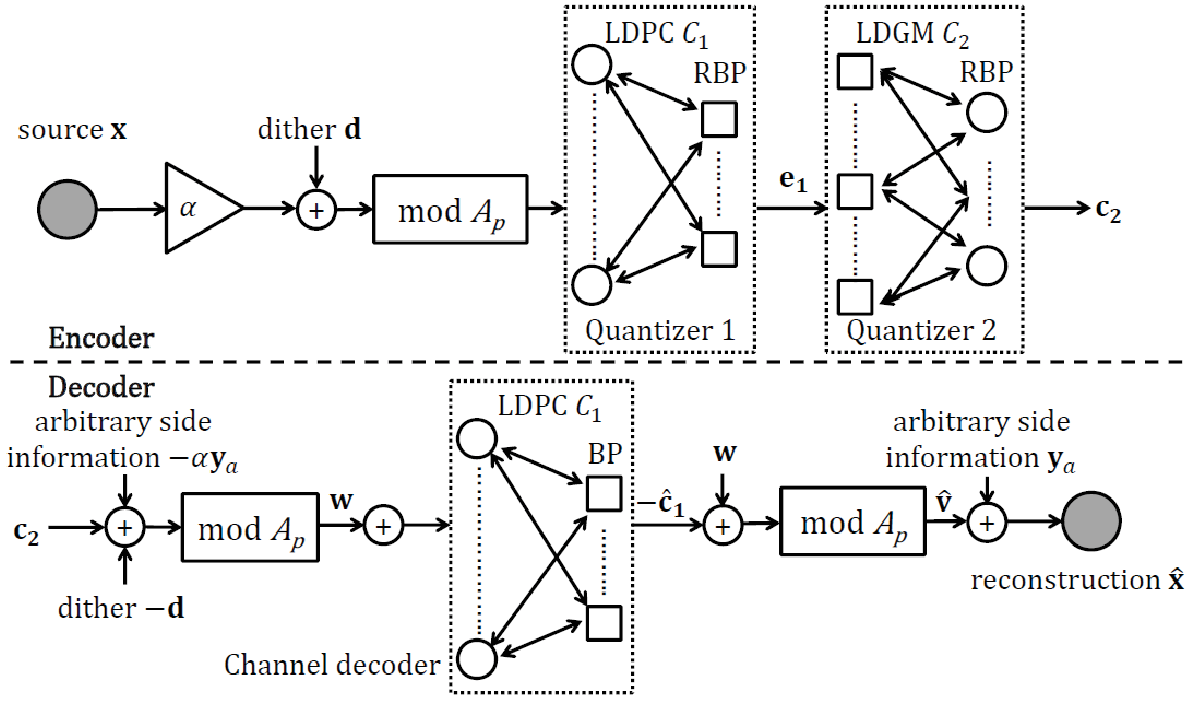
Theoretically, from [8], the $C_{1}$ must be a SSC code while $C_{2}$ must be a good source code. We implement $C_{1}$ and $C_{2}$ in Fig. 1 by an LDPC and an LDGM, respectively. The detailed block diagram of our practical implementation is shown in Fig. 2. Before introducing our flow to select the code parameters and the detailed encoding/decoding algorithms in Section III-B, in Section III-A, we first discuss some problems encountered when building our flow for the practical implementation.

III-A Issues for practical implementation

Finite modulo size : In [8], the Wyner-Ziv bound is achieved while the modulo size $A$ approaches infinity. However, infinite modulo size $A$ is impractical since the rate $R_{1}$ in (9) will become infinite, too. Thus we propose the following method to estimate how large $A$ should be in practice. From [8], the $\epsilon_{1}$ and $\epsilon_{2}$ in (9) satisfy

$$\epsilon_{2}<\epsilon_{1}=h(\alpha V-E_{2})-h((\alpha V-E_{2})\bmod A),$$ (12)

where $V\sim N(0,P_{V})$, and $E_{2}$ is a random variable corresponding to $\mathbf{e_{2}}$ in (5) in the Shannon-random coding setting. The distribution of $E_{2}$ is detailed in [8]. By numerically calculating the right-hand-side (RHS) of the equality in (12), we can choose $A$ to make $\epsilon_{1}$ and $\epsilon_{2}$ smaller than a threshold $\epsilon$.

In the following, we use the modulo size $A_{\epsilon}$ to represent the sufficiently large modulo size such that we can essentially neglect $\epsilon_{1}$ and $\epsilon_{2}$ in (9).

Channel decoding beyond capacity : With $A_{\epsilon}$ obtained previously, we can select $R_{1}$ from (9) by replacing $A$ with $A_{\epsilon}$ and neglect $\epsilon_{1}$. However, if we directly implement the channel decoder in Fig. 2 with selected $R_{1}$ and $A_{\epsilon}$, the channel decoder will always fail. The reason is as follows. Since no practical quantizers $C_{1}$ and $C_{2}$ can exactly achieve the rate-distortion bound, we will get the practical quantization error variance $D_{2,\epsilon}$ of ${\mathbf{e}}_{2}$ in (5) larger than the theoretical one predicted in [8]. From (6), the variance of the equivalent noise (7) will also be larger than the theoretical value in [8], which makes the selected $R_{1}$ operating in the regime above the channel capacity in (10) with $A=A_{\epsilon}$.

To solve the channel decoding beyond capacity problem described above, we propose a method which increases $A_{\epsilon}$ to $A_{p}$ while $R_{1}$ is fixed as that in Step 2 of Table I. The key idea is that the equivalent SNR at the channel decoder in Fig. 2 will also increase. To be more specific, from the random codebook construction in [8], we know that the optimal constellation of $C_{1}$ is uniformly distributed in $[-\frac{A_{\epsilon}}{2},\frac{A_{\epsilon}}{2}]$. Thus we use the uniform pulse amplitude modulation (PAM) as the constellation of $C_{1}$, and the equivalent SNR of the channel (6) with $A=A_{\epsilon}$ is

$$SNR_{\epsilon}=\frac{A_{\epsilon}^{2}/k}{D_{2,\epsilon}+\alpha^{2}P_{V}},$$ (13)

where $k$ is a constant related to the order of the PAM constellation. If we increase the modulo size from $A_{\epsilon}$ to $A_{p}$ with rates $R_{1}$ and $R_{2}$ unchanged, the quantization error variance of ${\mathbf{e}}_{2}$ in (5) will become

$$D_{2,p}=(A_{p}/A_{\epsilon})^{2}D_{2,\epsilon},$$ (14)

because the variance of $C_{1}$’s input, which is uniformly-distributed, will increase from $A_{\epsilon}^{2}/12$ to $A_{p}^{2}/12$. Then the equivalent SNR becomes

$$SNR_{p}=\frac{A_{p}^{2}/k}{D_{2,p}+\alpha^{2}P_{V}}=\frac{A_{\epsilon}^{2}/k}{D_{2,\epsilon}+(\frac{A_{\epsilon}}{A_{p}})^{2}\alpha^{2}P_{V}},$$

which is larger than $SNR_{\epsilon}$ in (13) since $A_{p}>A_{\epsilon}$.

Now we consider the loss of the practical channel decoder with practical $C_{1}$ in Fig. 2 compared to the optimal channel coding in [8]. For the practical channel coding, let $\sigma_{n,\epsilon}^{2}$ be the variance of the maximum tolerable equivalent noise for the successful decoding, where the PAM constellation of $C_{1}$ is chosen according to $A_{\epsilon}$. Then under the non-ideal channel decoding, we have

$$\sigma_{n,\epsilon}^{2}<D_{2,\epsilon}+\alpha^{2}P_{V},$$ (15)

where the RHS is the variance of the equivalent noise (7). When the PAM constellation of $C_{1}$ is chosen according to $A_{p}$ instead of $A_{\epsilon}$, the signal power of codeword $\mathbf{c_{1}}$ is scaled by $(A_{p}/A_{\epsilon})^{2}$. Then the maximum tolerable equivalent noise variance $\sigma_{n,p}^{2}$ for the practical channel coding can be estimated by

$$\sigma_{n,p}^{2}=(A_{p}/A_{\epsilon})^{2}\sigma_{n,\epsilon}^{2}.$$ (16)

Now we wish $\sigma_{n,p}^{2}\geq D_{2,p}+\alpha^{2}P_{V}$ to ensure the practical channel decoding in (6) being successful. Using this criterion with (14) and (16), the practical modulo size $A_{p}$ in Fig. 2 must meet,

$$A_{p}\geq(\frac{A_{\epsilon}^{2}\alpha^{2}P_{V}}{\sigma_{n,\epsilon}^{2}-D_{2,\epsilon}})^{\frac{1}{2}}.\vskip-2.84544pt$$ (17)

$\sigma_{n,\epsilon}^{2}$ and $D_{2,\epsilon}$ can be obtained via numerical simulations. From (15), we know that $A_{p}$ selected according to (17) is lager than $A_{\epsilon}$. Although increasing the modulo size can solve the channel decoding beyond capacity problem, there will be a loss in the final distortion compared with the theoretically predicted $D$ using $R_{2}$ in (11) owing to the increment of the quantization error variance of ${\mathbf{e}}_{2}$ in (5) from (14).

Edge degree for SSC LDPC : One of the critical parts of our residual WZC is the requirement of a practical SSC code $C_{1}$. The best known SSC so far is the trellis coded quantation (TCQ)/modulation. However, according to the simulation results in [15], using TCQ as our $C_{1}$ will result in significant performance loss compared with the Wyner-Ziv bound. Alternatively, in [12], LDPC was proved to be an SSC code for the binary source/channel under the optimal encoder/decoder. However, the theoretical proof in [12] gives no hints for the edge degree design and the practical quantization algorithms for SSC LDPC. Recently, the RBP algorithm was proposed in [13] for the quantization of the binary source with LDPC. However, the LDPC in [13] is not SSC, since its edge degree exhibits the ultra-sparse structure which makes LDPC poor for the channel coding when the belief-propagation (BP) algorithm [16] is used.

To solve the practical design problem for SSC LDPC, we propose using LDPC with the edge degree optimized for the channel coding, and modifying the binary RBP in [13] for our continuous LDPC quantization with mod-A operation. Although our edge degree for the first-stage quantizer $C_{1}$ in Fig. 2 is sub-optimal for the source coding, our simulation results show that it suffices to make the overall residual WZC approach the Wyner-Ziv bound. Indeed, our simulation results in Section IV-A show that our LDPC has a shaping loss [9] about only 0.5 dB away from the rate-distortion bound when the quantizer input is uniformly-distributed. Our modified RBP algorithm is given in Sec. III-B.

III-B Design flow and encoding/decoding algorithms

Our overall design flow is summarized in Table I and is explained in detail as follows. The Step 1 and 2 in Table I are described previously in Sec. III-A. To design the edge degree of the SSC LDPC in Step 3, as discussed in Sec. III-A, we adopt the EXIT chart fitting approach in [17] to obtain an LDPC good for the channel coding. By running the BP channel decoding algorithm, we can calculate the $\sigma^{2}_{n,\epsilon}$ described before (15) for our LDPC with the PAM constellation points. For Step 4, the rate of the LDGM is given in (11), and the quantization alphabet is uniformly spaced with energy $\alpha^{2}P_{V}$ suggested in [8]. The edge degree of LDGM is obtained similarly as in [18].

To calculate $D_{2,\epsilon}$ in Step 4 of Table I, we modify the RBP in [13] as the quantization algorithm for both LDPC and LDGM at the WZC encoder in Fig. 2. The RBP is a generalization of BP by adding an reinforcement term controlled by the constants $\gamma_{0},\gamma_{1}\in[0,1]$ to the marginal $L$-value calculated from the variable nodes (VND) of the graph-based code. The main modification of our RBP algorithm is the a priori information from the source. Taking quantizer $C_{1}$ as an example. We let $u_{i}$ be the $i$th element of $C_{1}$’s input (uniform), and $c_{1,i}$ be the $i$th coded symbol of codeword $\mathbf{c_{1}}$. To reflect the modulo $A_{\epsilon}$ operation before $C_{1}$ in Fig. 1, we use the following conditional probability density function (PDF) to calculate the a priori information

$$f_{u_{i}|c_{1,\;i}}=\sum_{b\in\mathbb{Z}}f_{G,\sigma_{n,\epsilon}^{2}}(u_{i}-c_{1,i}+A_{\epsilon}b),$$ (18)

where $f_{G,\sigma_{n,\epsilon}^{2}}(g)$ is the PDF of $N(0,\sigma_{n,\epsilon}^{2})$, and $\mathbb{Z}$ is the integer set. The rest of the algorithm is the same as that in [13] and is omitted here. After obtaining $D_{2,\epsilon}$ in Step 4, we can follow Step 5, which is described in Sec. III-A, to get the practical modulo size $A_{p}$ in Fig. 2 and complete our design.

Finally, note that the complexity of the BP channel decoding algorithm for our WZC decoder is linear [16] in codelength (i.e. $O(n)$), also is the RBP algorithm used in our WZC encoder. Adopting the RBP algorithm instead of the $O(n^{2})$ hard-decimation-based one in [14][18] significantly reduces our computation complexity.

TABLE I: Design Flow of Residual WZC

1:	Determine the target (ideal) MSE distortion $D$:
	Given $P_{V}$ and WZC rate $R_{2}$, determine $D$ from (11)
2:	Determine code rate $R_{1}$ of the 1st-stage quantizer:
	Given $\epsilon$, find $A=A_{\epsilon}$ such that $\epsilon_{1}<\epsilon$ from (12).
	Compute $R_{1}$ from (9) with $A=A_{\epsilon}$.
3:	Find the maximum tolerable noise variance $\sigma^{2}_{n,\epsilon}$ of the channel
	decoder with $A=A_{\epsilon}$:
	Design SSC LDPC with rate $R_{1}$. Calculate $\sigma^{2}_{n,\epsilon}$ with BP.
4:	Find the distortion $D_{2,\epsilon}$ of the 2nd-stage $C_{2}$ with $A=A_{\epsilon}$
	Design LDGM with rate $R_{2}$.
	Calculate $D_{2,\epsilon}$ with modified RBP applied to LDPC and LDGM.
5:	Determine the practical modulo size $A_{p}$:
	Calculate $A_{p}$ using the RHS of (17). If the LDPC decoder fails,
	increase $A_{p}$ until it succeeds. Test the final MSE with the final $A_{p}$.

IV Design example and Discussions

In our design example, different from the Gaussian side information in [10][19], we let each element of the side information ${\mathbf{y}}$ in (1) be uniformly distributed in $[-A/2,A/2]$. Due to the dither, the distribution of ${\mathbf{y}}$ will not affect our performance. The details of our design example is given in Sec. IV-A, with the distortion performance given in the end of this subsection. Finally, Sec. IV-B provides more discussions on our work.

IV-A Design example with detailed code parameters selection

Following our design flow in Table I, we first set $P_{V}$ in (3) as $0.28$ and the WZC rate $R_{2}=0.953$, and then the ideal distortion $D$ is 0.0747. For Step 2, given $\epsilon$=0.005, we find that choosing $A_{\epsilon}$ as $3$ is sufficient. $R_{1}$ is $0.68$ bpcu. For Step 3, we use 2-PAM LDPC to implement $C_{1}$ with constellation points $\pm\frac{A_{\epsilon}}{4}$. To achieve the WZC bound, we choose codeword length $n=10^{5}$ symbols per source block. The degree profile is : check nodes (CND): $100\%$ of degree 12; VND: $35.36\%$ of degree 2, $44.74\%$ of degree 3, and $19.89\%$ of degree 9. By applying the BP channel decoding algorithm, we obtain $\sigma^{2}_{n,\epsilon}$ as 0.185.

For Step 4, we adopt 4-ary LDGM where every two bits of the LDGM CND are Gray-mapped to a 4-ary symbol. The degree profile can be found in [18]. By running the RBP quantization algorithm with $\gamma_{0}=1$, $\gamma_{1}=0.99980$ at the LDPC and LDGM, we obtain $D_{2,\epsilon}$ as 0.0577. The Monte Carlo simulation tests 2000 blocks of uniformly-distributed source samples and 3000 iterations are run for each source block. The summation over integer set $\mathbb{Z}$ in (18) is obtained by limiting $|b|\leq 3,b\in\mathbb{Z}$. As in [13], in some few cases the RBP algorithm diverges, i.e. not all the constraints of CND are satisfied. For these few cases, as in [13], restarting the RBP by adding 0.00001 to $\gamma_{1}$ will solve the problem. Finally, from Step 5, we calculate the lower-bound of $A_{p}$ in (17) as 3.261. The bit error rate of LDPC is smaller than $10^{-4}$ when the modulo size $A_{p}$ is 3.29.

Finally, we run the Monte Carlo simulation to test 2000 source blocks. The distortion loss compared with the ideal $D$ is 0.995 dB at the WZC rate 0.9531 b/s. The best simulation result known with $P_{V}=0.28$ [10], which is only for the Gaussian side information, has 1.07 dB loss at the rate 1.07 b/s and block length $n=10^{5}$. The results in [10] are obtained using 8192-state trellis coded quantization (TCQ) and 3-stage SWC (three LDPCs in the SWC encoder). Our work is as competitive as [10]. Besides, our SSC LDPC has only 0.48 dB SNR loss compared to the capacity and 0.43 dB shaping loss compared to the rate-distortion bound. More design examples can be found in [20].

IV-B Detailed comparison

Although the well-known practical WZC design [10] also performs a two-stage quantization/cpmpression process, the second stage quantizer/compressor in [10] is lossless with input being the quantization output of the first stage. In our residual WZC, the second stage quantizer is lossy with input being the quantization error of the first stage, and thus the decoder structure is also different from that in [10]. Compared with the WZC in [10], the main advantage of our coding scheme is the flexibility. Firstly, as shown in [8], our residual WZC can approach the Wyner-Ziv bound with arbitrary side information in all rate regimes, while the WZC in [10][11] can only guarantee the optimality in high rate regimes. In [10], the lower the WZC rate the more severe the rate loss is. Secondly, our construction offers more flexibility in the practical code rate selection. In [10], the WZC is implemented by a rate $R_{N}$ TCQ and a multilevel SWC (formed by $R_{N}$ LDPCs). The rate of TCQ $R_{N}$ is limited to be an integer, and for each $R_{N}=1,2,\ldots$, only one possible WZC rate can be implemented. However, almost all the rational WZC rates can be implemented by our construction.

Our construction is also different from and more flexible than the graph-based construction in [6] for which the encoder codebook is nested. Moreover, the WZC in [6] has only been proven to be optimal for the binary symmetric source with Hamming distortion measure. Whether it can be extended to the quadratic-Gaussian case as considered in this paper or not is still unknown. Finally, our simulation results show that LDPC itself suffices to be a good SSC code, thus the compound LDGM/LDPC construction proposed in [6] may not be necessary for our first-stage quantizer $C_{1}$.

V Conclusion

In this paper, we considered the quadratic-Gaussian Wyner-Ziv problem where side information can be arbitrarily distributed. We implemented the theoretically-claimed residual WZC by LDPC and LDGM. We identified and solved a problem called the channel decoding beyond capacity problem when designing our practical decoder. Moreover, we modified the RBP algorithm to make the LDPC with the edge degree optimized for the channel coding perform well as a source code. The simulation results showed that our practical construction approaches the Wyner-Ziv bound, and has a similar performance compared with previous works. Moreover, our construction can offer more design flexibility in terms of the distribution of the side information and the practical code rate selection.

References

- [1] A. D. Wyner, “The rate-distortion function for source coding with side information at the decoder-II: General sources,” Inf. Contr., vol. 38, pp. 60–80, Jan. 1978.
- [2] D. Slepian and J. K. Wolf, “Noiseless coding of correlated information sources,” IEEE Trans. Inform. Theory, vol. 19, no. 4, pp. 471–480, July 1973.
- [3] Z. Xiong, A. D. Liveris, and S. Cheng, “Distributed source coding for sensor networks,” IEEE Signal Processing Mag., vol. 21, no. 5, pp. 80–94, Sep. 2004.
- [4] R. Zamir, S. Shamai(Shitz), and U. Erez, “Nested linear/lattice codes for structured multiterminal binning,” IEEE Trans. Inform. Theory, vol. 48, no. 6, pp. 1250–1276, Jun. 2002.
- [5] G. Kramer, M. Gastpar, and P. Gupta, “Cooperative strategies and capacity theorems for relay networks,” IEEE Trans. Inform. Theory, vol. 51, no. 9, pp. 3037–3063, Sep. 2005.
- [6] M. J. Wainwright and E. Martinian, “Low-density graph codes that are optimal for binning and coding with side information,” IEEE Trans. Inform. Theory, vol. 55, no. 3, pp. 1061–1079, Mar. 2009.
- [7] S. B. Korada and R. L. Urbanke, “Polar codes are optimal for lossy source coding,” IEEE Trans. Inform. Theory, vol. 56, no. 4, pp. 1751–1768, Apr. 2010.
- [8] S.-J. Lin, S.-C. Lin, K.-S. Chen, and H.-J. Su, “Coding for noisy quadratic-Gaussian Wyner-Ziv problem: A successive quantization approach,” in IEEE Information Theory Workshop, 2009.
- [9] A. Gersho and R. M. Gray, Vector quantization and signal compression. Kluwer Academic Fublishers, 1992.
- [10] Y. Yang, S. Cheng, Z. Xiong, and W. Zhao, “Wyner-Ziv coding based on TCQ and LDPC codes,” IEEE Trans. Commun., vol. 57, no. 2, pp. 376–387, Feb. 2009.
- [11] Z. Liu, S. Cheng, A. D. Liveris, and Z. Xiong, “Slepian-Wolf coded nested lattice quantization for Wyner-Ziv coding: High-rate performance analysis and code design,” IEEE Trans. Inform. Theory, vol. 52, no. 10, pp. 4358–4379, Oct. 2006.
- [12] V. Chandar, “Sparse graph codes for compression, sensing, and secrecy,” Ph.D. dissertation, Massachusetts Institute of Technology, June 2010.
- [13] A. Braunstein, F. Kayhan, and R. Zecchina, “Efficient data compression from statistical physics of codes over finite fields,” Phys. Rev. E, vol. 84, p. 051111, Nov 2011. [Online]. Available: http://link.aps.org/doi/10.1103/PhysRevE.84.051111
- [14] T. Filler and J. Fridrich, “Binary quantization using belief propagation with decimation over factor graphs of LDGM codes,” in 45th Annual Allerton Conf. on Comm. Control, and Comput., Monticello, IL, USA, 2007.
- [15] K.-S. Chen, “Low density constructions for simultaneously good for channel and source coding problem with applications,” Master’s thesis, National Taiwan university, 2009.
- [16] D. J. C. MacKay, “Good error-correcting codes based on very sparse matrices,” IEEE Trans. Inform. Theory, vol. 45, no. 2, pp. 399–431, March 1999.
- [17] S. ten Brink, G. Kramer, and A. Ashikhmin, “Design of low-density parity-check codes for modulation and detection,” IEEE Trans. Commun., vol. 52, no. 4, pp. 670–678, Apr. 2004.
- [18] Q. Wang and C. He, “Approaching 1.53-dB shaping gain with LDGM quantization codes,” in IEEE Global Telecommunications Conference, 2007, pp. 1571–1576.
- [19] S. S. Pradhan and K. Ramchandran, “Distributed source coding using syndromes (DISCUS): Design and construction,” IEEE Trans. Inform. Theory, vol. 49, no. 3, pp. 626–643, Mar. 2003.
- [20] Y.-P. Wei, S.-C. Lin, S.-J. Lin, and H.-J. Su, “Residual-quantization based code design for source coding with arbitrary decoder side information,” to be submitted to IEEE Trans. Inform. Theory.