Current loops and fluctuations in the zero-range process on a diamond lattice

Abstract

We study the zero-range process on a simple diamond lattice with open boundary conditions and determine the conditions for the existence of loops in the mean current. We also perform a large deviation analysis for fluctuations of partial and total currents and check the validity of the Gallavotti-Cohen fluctuation relation for these quantities. In this context, we show that the fluctuation relation is not satisfied for partial currents between sites even if it is satisfied for the total current flowing between the boundaries. Finally, we extend our methods to study a chain of coupled diamonds and demonstrate co-existence of mean current regimes.

, ,

Keywords: current fluctuations, large deviations in non-equilibrium systems, stochastic particle dynamics (theory), zero-range processes

1 Introduction

In the last decades much effort has been put into understanding and modelling non-equilibrium systems, which find applications in fields ranging from biology to finance [1, 2]. Among the various models which have been proposed to study such real-life processes, stochastic interacting particle systems (interacting Markov systems) have enjoyed particular success [3]. In this class, the zero-range process (ZRP) is a well studied lattice gas model offering many applications and the possibility of obtaining analytical results. Introduced in 1970 [4], one of the reasons the ZRP gained interest was because it can show a phase transition from a fluid to a condensed state [5]. The ZRP has been extensively studied with both periodic and open boundary conditions in one dimension [6, 7], and some variants involving junction topologies have also been introduced, see e.g. [8, 9]. Furthermore, currents in a closely related model have recently been considered on more general networks [10], which may give some insight into expected effects for manmade networks such as traffic on roads or the internet.

For extended ZRPs defined on two-dimensional or three-dimensional lattices, particle currents can flow in principle in loops within the bulk of the system. To illustrate this possibility, we study a simple variant of the ZRP defined on a diamond-shaped lattice with open boundaries. For this model, we are able to obtain analytical expressions for the mean current flowing between specific sites of the lattice which show that the model has two regimes of mean particle currents: a unidirectional regime where particles flow in the same direction through different lattice branches and a loop current regime where the mean current flows around the diamond. The analysis is also extended to a chain of coupled diamonds where, for a weak asymmetry of the bulk hopping rates, we find a transition between unidirectional and loop current regimes persisting in the large-system-size limit.

In addition to mean currents, we also study fluctuations by calculating the probability distribution of particle currents and its associated large deviation rate function, which plays a role similar to thermodynamic potentials in equilibrium systems [11, 12]. Recently much experimental and theoretical attention has been devoted to the study of certain fluctuation symmetries [13, 14], which may also be observed experimentally, e.g. [15, 16]. Our simple model allows us to study explicitly the joint probability of observing a given current on different lattice branches. We obtain analytically the large deviation functions for currents across different bonds and hence gain understanding of the role of current loops. These results for current loops, which are difficult to obtain for general models, are expected to be important in testing fluctuation symmetries for higher dimensional systems, such as those reported recently by Hurtado et al. [17].

The remainder of the paper is structured as follows. In section 2, we define the ZRP on the diamond lattice and calculate its stationary state. In section 3, we discuss the appearance of unidirectional and loop mean current regimes in the system. In section 4, we calculate the joint particle current fluctuations of the upper and lower branches of the lattice and test the well known Gallavotti-Cohen fluctuation relation for partial and total currents. In section 5 we use our approach to analyse a chain of diamonds. Finally, in section 6, we discuss our results and their possible implications for other models.

2 Zero-range process on a diamond lattice

2.1 Definition of model

The ZRP is a lattice-based many-particle model in which, as the name suggests, particles interact only with other particles at the same site. Additionally, particles are allowed to accumulate to any non-negative number on each site of the lattice. Here, we study the ZRP with open boundary conditions on a diamond lattice as shown in figure 1.

Figure 1: Diamond array. The $z_{i}$’s represent the fugacities of sites 1–4. The quantities $\alpha$, $\gamma$, $\delta$, $\beta$, $p$ and $q$ are the hopping rates.

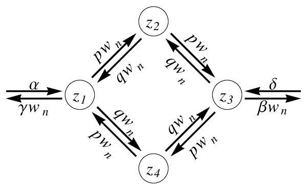
The dynamics of the particles on this lattice is defined in continuous time such that the topmost particle on each site hops to an adjacent site after an exponentially distributed waiting time. More precisely, particles hop clockwise around the diamond with rate $pw_{n}$ and anti-clockwise with rate $qw_{n}$, where the interaction between particles on each site is taken into account by the term $w_{n}$ which depends exclusively on the occupation number $n$ of the departure site. Given the symmetry of the system, without loss of generality we will assume from now on that

$$p\geq q.$$ (1)

Moreover, we allow particles to enter and leave the boundary sites with probability rates $\alpha$ and $\beta w_{n}$ for site 1, $\delta$ and $\gamma w_{n}$ for site 3.

Based on the one-dimensional open boundary ZRP studied in [7] we expect the system to be driven out of equilibrium for $\alpha/\gamma\neq\delta/\beta$ but that some choices of parameters may lead to a boundary condensation phenomenon in which particles accumulate on one of the sites 1 or 3. We shall return to this point later.

In the quantum Hamiltonian formalism [18], one defines a probability vector

$$|P\rangle=\sum\limits_{n}P(n)|n\rangle$$ (2)

where $|n\rangle$ is a basis vector for the particle configuration $n=(n_{1},n_{2},n_{3},n_{4})$ and $P(n)$ the probability of that configuration. Then the time evolution of the system is described by the master equation

$$\frac{d|P\rangle}{dt}=-H|P\rangle.$$ (3)

Here the matrix $H$, or Hamiltonian, is the stochastic generator of the system. To explicitly write the Hamiltonian of our system we define the creation and annihilation operators on site $i$ by

$$a_{i}^{+}=\left(\begin{array}[]{cccc}0&0&0&\\ 1&0&0&\dots\\ 0&1&0&\\ &\vdots&&\ddots\end{array}\right)\text{ and }a_{i}^{-}=\left(\begin{array}[]{cccc}0&w_{1}&0&\\ 0&0&w_{2}&\dots\\ 0&0&0&\\ &\vdots&&\ddots\end{array}\right)$$ (4)

respectively. With the additional definition of the diagonal matrix $d_{i}=w_{j}\delta_{j,k}$, the Hamiltonian of the model shown in figure 1 is written

$$-H= \alpha\left(a_{1}^{+}-1\right)+\gamma\left(a_{1}^{-}-d_{1}\right)+\delta\left(a_{3}^{+}-1\right)+\beta\left(a_{3}^{-}-d_{3}\right)$$ (5)

$$+\sum\limits_{k=1}^{4}p\left(a_{k}^{-}a_{k+1}^{+}-d_{k}\right)+q\left(a_{k}^{+}a_{k+1}^{-}-d_{k+1}\right)$$

where the index sums are taken modulo 4.

2.2 Steady state

We are interested in finding the non-equilibrium stationary state $|P^{*}\rangle$ of our system. By definition, this probability does not change in time and is therefore, such that

$$H|P^{*}\rangle=0.$$ (6)

It has been shown that for the ZRP on any lattice geometry the steady state factorises as the tensor product (see, e.g., [19])

$$|P^{*}\rangle=|P_{1}^{*}(n_{1})\rangle\otimes|P_{2}^{*}(n_{2})\rangle\otimes...\otimes|P_{L}^{*}(n_{L})\rangle.$$ (7)

Here each site’s probability distribution vector is given by

$$|P_{k}^{*}(n_{k})\rangle=\sum\limits_{n_{k}}P_{k}(n_{k})|n_{k}\rangle,$$ (8)

with $P_{k}(n_{k})$ the probability of finding $n_{k}$ particles on the $k$th-site and $|n_{k}\rangle$ the corresponding configuration vector. Furthermore, $P_{k}(n_{k})$ is given in terms of the site’s fugacity $z_{k}$ and the interaction term $w_{n}$ by

$$P_{k}(n_{k})=Z_{k}^{-1}z_{k}^{n_{k}}\prod\limits_{i=1}^{n_{k}}w_{i}^{-1},$$ (9)

where $Z$ is the grand canonical partition function

$$Z_{k}=\sum\limits_{j=0}^{\infty}z_{k}^{j}\prod\limits_{l=1}^{j}w_{l}^{-1}.$$ (10)

It now becomes obvious that the choice of the interaction $w_{n}$ will be reflected in the existence of the partition function. For instance, if we let

$$\lim\limits_{n\rightarrow\infty}w_{n}=\kappa,$$ (11)

with $\kappa$ a constant, then we have to make sure that $z<\kappa$ in order for the infinite sum of equation (10) to converge and the partition function to exist. Hopping parameters leading to $z>\kappa$ correspond physically to a growing condensate. In the remainder of this paper we will assume, unless stated otherwise, an unbounded interaction rate $w_{n}$ for the particles, i.e.,

$$\lim\limits_{n\rightarrow\infty}w_{n}=\infty.$$ (12)

This guarantees that the system has a non-equilibrium stationary state without condensation.

It can be shown that the creation and annihilation operators act on the stationary-state eigenvector of the Hamiltonian as $a_{k}^{+}|P_{k}^{*}\rangle=z_{k}^{-1}d_{k}|P_{k}^{*}\rangle$ and $a_{k}|P^{*}_{k}\rangle=z_{k}|P_{k}^{*}\rangle$ respectively. Here we have made explicit that the operators corresponding to the $k$th-site act only on the probability distribution vector of the same site. Thus, applying the Hamiltonian (5) to the stationary state vector $|P^{*}\rangle$ yields the expression

$$H|P^{*}\rangle= -\left[\left(\alpha-\gamma z_{1}+qz_{2}-pz_{1}+pz_{4}-qz_{1}\right)z_{1}^{-1}d_{1}\right.$$ (13)

$$+\left(pz_{1}-qz_{2}+qz_{3}-pz_{2}\right)z_{2}^{-1}d_{2}$$

$$+\left(\delta-\beta z_{3}+pz_{2}-qz_{3}+qz_{4}-pz_{3}\right)z_{3}^{-1}d_{3}$$

$$+\left(qz_{1}-pz_{4}+pz_{3}-qz_{4}\right)z_{4}^{-1}d_{4}$$

$$\left.-\left(\alpha-\gamma z_{1}+\delta-\beta z_{3}\right)\right]|P^{*}\rangle$$

and for $|P^{*}\rangle$ to be the required stationary state the coefficients of the matrices $d_{i}$ must vanish. Solving the resulting system of equations leads to the fugacities

$$z_{1}=\frac{(p+q)\alpha\beta+(p^{2}+q^{2})(\alpha+\delta)}{(p+q)\beta\gamma+(p^{2}+q^{2})(\beta+\gamma)},$$

$$z_{2}=\frac{p\alpha\beta+q\gamma\delta+(p^{2}+q^{2})(\alpha+\delta)}{(p+q)\beta\gamma+(p^{2}+q^{2})(\beta+\gamma)},$$

$$z_{3}=\frac{(p+q)\gamma\delta+(p^{2}+q^{2})(\alpha+\delta)}{(p+q)\beta\gamma+(p^{2}+q^{2})(\beta+\gamma)},$$

$$z_{4}=\frac{q\alpha\beta+p\gamma\delta+(p^{2}+q^{2})(\alpha+\delta)}{(p+q)\beta\gamma+(p^{2}+q^{2})(\beta+\gamma)}.$$ (14)

Note that with these solutions, one verifies that $\alpha-\gamma z_{1}+\delta-\beta z_{3}=0$, which is consistent with the stationary state being the eigenvector with eigenvalue zero.

With these fugacities, we can calculate the mean time-averaged current $\bar{j}_{a,b}$ which measures the average number of particles jumping from site $a$ to site $b$ per unit time. This current is expressed in terms of the fugacities as

$$\bar{j}_{k,k+1}=pz_{k}-qz_{k+1}=-\bar{j}_{k+1,k}.$$ (15)

Here once again, $k\in\left\{1,2,3,4\right\}$ and modulo 4 applies over the subindex addition. Similarly, for the boundary sites the mean current is

$$\bar{j}_{L}=\alpha-\gamma z_{1},$$

$$\bar{j}_{R}=\beta z_{3}-\delta,$$ (16)

with the convention of a positive flow direction from the left to the right boundary of the lattice.

Since we have assumed the system is in a stationary state without condensation, the mean currents must satisfy

$$\bar{j}_{L}=\bar{j}_{1,2}+\bar{j}_{1,4}=\bar{j}_{2,3}+\bar{j}_{4,3}=\bar{j}_{R}$$ (17)

by particle conservation. From this we then find that the mean current at the left boundary is positive if

$$\alpha-\gamma z_{1}>0,\\$$

which is equivalent to

$$\frac{\left(p^{2}+q^{2}\right)\left(\alpha\beta-\gamma\delta\right)}{\left(p+q\right)\beta\gamma+\left(p^{2}+q^{2}\right)\left(\beta+\gamma\right)}>0\\$$

or

$$\alpha\beta-\gamma\delta>0.$$ (18)

This condition implies a net current left-to-right through the system. If conditions (1) and (18) are satisfied, it follows that the largest fugacity is $z_{1}$. Hence, returning to the discussion of a bounded interaction $w_{n}$, the consistency condition for existence of a stationary state without condensation is $z_{1}<\kappa$.

3 Particle current loops

An interesting feature of the model we are studying is that it shows a transition from a unidirectional mean current to a loop mean current regime as the parameters are varied – see figure 2. An intuitive way to see this change, is to consider specific parameter values. On one hand, when we have symmetric hopping rates $p=q=1$, the mean current flows clockwise through the upper branch and anti-clockwise through the lower branch, i.e., the unidirectional regime. On the other hand, when we have completely asymmetric hopping rates $p=1$ and $q=0$, the mean current flow is forced to go around the diamond, i.e., the loop current regime. Since the mean current through the lower branch changes from anti-clockwise to clockwise direction as the regime changes from unidirectional to a loop, one way to determine where the transition occurs is to calculate the parameters at which the mean current $\bar{j}_{1,4}$ between sites 1 and 4 vanishes.

Figure 2: Two regimes: Unidirectional (left) and loop mean currents (right).

As a first step to characterize this change of regime in more detail we now consider the special case of $\gamma=\delta=0$, which corresponds to having only injection of particles at the left end of the lattice and only depletion at the right end. This allows us to understand the change of regime with fewer parameters and get some intuition for the cases with non-zero hopping rates $\gamma$ and $\delta$.

From equations (14) and (15) the condition for a vanishing mean current $\bar{j}_{1,4}$ is satisfied when

$$B=\frac{-Q^{3}+Q^{2}-Q+1}{Q^{2}},$$ (19)

where we have defined the ratios $Q=q/p$ and $B=\beta/p$. The curve defined by the equation above gives us the exact location of the regime change from positive to negative average current as shown in figure 3. As expected, if $Q=0$ (i.e., $q=0$) it does not matter how large the extraction rate $B$ (or $\beta$) is, the system is always in the loop regime, whereas if $Q=1$ (i.e., for symmetric hopping rates) the system is always in the unidirectional regime. Notice also that equation (19) has no dependence on the injection parameter $\alpha$ which means, that for $0<Q<1$ we can control the system regime just by changing the extraction rate $\beta$. For large $\beta$, the system favours the unidirectional regime whereas, for low $\beta$, a smaller fraction of the particles on site 3 can leave the system and a loop current is therefore more likely.

Figure 3: Regimes of the average current $\bar{j}_{1,4}$. Red region $\bar{j}_{1,4}<0$. Blue region $\bar{j}_{1,4}>0$

In the general case where we admit injection and extraction of particles from both boundary sites, we can still compute the mean current $\bar{j}_{1,4}$:

$$\bar{j}_{1,4}=\frac{(\alpha+\delta)\left(p^{2}+q^{2}\right)\left(q-p\right)+\alpha\beta q^{2}-\gamma\delta p^{2}}{(p^{2}+q^{2})(\beta+\gamma)+(p+q)\beta\gamma}.$$ (20)

We can check again that for the special cases of symmetric hopping rates (i.e., $p=q=1$) the current is positive and the system is in the unidirectional regime, whereas for totally asymmetric rates (i.e., $p=1$ and $q=0$) the current is negative and thus, in the loop current regime as expected. Moreover, for fixed $p>q>0$, we can see that the mean current regime can be chosen by changing the boundary rates where, just as in the special case discussed above, large $\beta$ favours the unidirectional regime and small $\beta$ the loop current regime. Similarly, for fixed boundary conditions satisfying $\alpha\beta>\gamma\delta$, we can choose the mean current regime by varying the bulk hopping rates $p$ and $q$. A further remark about the existence of these two regimes, is that if we were to consider $w_{n}$ bounded we know that for some choices of the hopping rates the system would undergo condensation (and have no steady state) meaning, for example, that not all of the phase plane in figure 3 would be accessible.

4 Particle current fluctuations

4.1 Large deviations

We now complement our results for the mean currents by studying their fluctuations. To be specific, we are interested in calculating the probability distribution $p(j_{a,b},t)$ of the time-averaged current $j_{a,b}$ between sites $a$ and $b$ in the lattice. In the long-time limit, we expect this distribution to follow the large deviation principle

$$p(j_{a,b},t)\sim\exp\left(-t\hat{e}(j_{a,b})\right),$$ (21)

with rate function (RF) $\hat{e}(j_{a,b})$. Here “$\sim$” denotes asymptotic equality in the limit of large time. One way to obtain the RF is to calculate the scaled cumulant generating function (SCGF)

$$e(\lambda)=\lim\limits_{t\rightarrow\infty}-\frac{1}{t}\log\langle e^{-\lambda tj_{a,b}}\rangle.$$ (22)

Indeed, if the SCGF is continuous and differentiable, then it is known that the RF is obtained from the SCGF via the Legendre transform [11] as

$$\hat{e}(j_{a,b})=\max\limits_{\lambda}\left\{e(\lambda)-\lambda j_{a,b}\right\}.$$ (23)

To calculate the SCGF we need to modify the Hamiltonian (5) to count particle jumps. This is done by multiplying the terms accounting for the transfer of particles from sites $a$ to $b$ (and vice versa) by the exponential factor $e^{\mp\lambda}$, see for example [13, 20, 21]. Then for instance, to measure the fluctuations of $\bar{j}_{1,4}$ the required modified Hamiltonian is:

$$-\hat{H}= \alpha\left(a_{1}^{+}-1\right)+\gamma\left(a_{1}^{-}-d_{1}\right)+\delta\left(a_{3}^{+}-1\right)+\beta\left(a_{3}^{-}-d_{3}\right)$$ (24)

$$+\sum\limits_{k=1}^{4}p\left(a_{k}^{-}a_{k+1}^{+}e^{\lambda\delta_{k,4}}-d_{k}\right)+q\left(a_{k}^{+}a_{k+1}^{-}e^{-\lambda\delta_{k,4}}-d_{k+1}\right).$$

The SCGF can be identified with the lowest eigenvalue of the Hamiltonian (24), which in general is different from zero. Then we find the desired RF of the current $j_{1,4}$ via the Legendre transform (23).

4.2 Joint probability of current fluctuations

Correlations between particle currents flowing through different bonds can be studied by considering a two-parameter SCGF. For the diamond lattice, it is interesting for example to study the current flowing between sites 1 and 2 and the current flowing between sites 1 and 4 simultaneously. The joint SCGF that characterizes the joint distribution $p\left(j_{1,2},j_{1,4},t\right)$ of these currents is calculated analytically by modifying the system’s Hamiltonian similarly to described above. Particle jumps between sites 1 and 2 are counted with parameter $\lambda_{1,2}$ and between sites 1 and 4 with parameter $\lambda_{1,4}$. This calculation leads to the two-parameter SCGF,

$${e(\lambda_{1,2},\lambda_{1,4})}={\frac{\left(Q+1\right)\left(\left(\alpha B+\delta Ge^{\lambda_{1,2}+\lambda_{1,4}}\right)\left(Q^{2}e^{\lambda_{1,2}}+e^{\lambda_{1,4}}\right)-\left(\alpha B+\delta G\right)\left(Q^{2}+1\right)e^{\lambda_{1,2}+\lambda_{1,4}}\right)}{Q^{4}e^{2\lambda_{1,2}}+e^{2\lambda_{1,4}}-e^{\lambda_{1,2}+\lambda_{1,4}}\left(1+Q^{4}+B\left(Q+1\right)\left(Q^{2}+1\right)+G\left(Q+1\right)\left(Q^{2}+BQ+B+1\right)\right)}}$$

$${+\frac{\left(\alpha+\delta\right)\left(Q^{4}e^{2\lambda_{1,2}}-e^{\lambda_{1,2}+\lambda_{1,4}}\left(Q^{4}+1\right)+e^{2\lambda_{1,4}}\right)}{Q^{4}e^{2\lambda_{1,2}}+e^{2\lambda_{1,4}}-e^{\lambda_{1,2}+\lambda_{1,4}}\left(1+Q^{4}+B\left(Q+1\right)\left(Q^{2}+1\right)+G\left(Q+1\right)\left(Q^{2}+BQ+B+1\right)\right)}}$$ (25)

where we have defined $Q=q/p$, $B=\beta/p$ and $G=\gamma/p$. For the special case $\gamma=\delta=0$ the SCGF reduces to

$$e(\lambda_{1,2},\lambda_{1,4})={\alpha\left(1+\frac{B(1+Q)(e^{\lambda_{1,4}}+e^{\lambda_{1,2}}Q^{2})}{e^{2\lambda_{1,4}}+e^{2\lambda_{1,2}}Q^{4}-e^{\lambda_{1,2}+\lambda_{1,4}}(Q^{4}+1+(1+Q)(1+Q^{2})B)}\right)}.$$ (26)

The RF $\hat{e}(j_{1,2},j_{1,4})$ associated with the joint distribution $p\left(j_{1,2},j_{1,4},t\right)$ is obtained from this SCGF via the double Legendre transform:

$$\hat{e}(j_{1,2},j_{1,4})=\max\limits_{\lambda_{1,2},\lambda_{1,4}}\left\{e(j_{1,2},j_{1,4})-j_{1,2}\lambda_{1,2}-j_{1,4}\lambda_{1,4}\right\}.$$ (27)

The numerical evaluation of this transform is shown in figure 4.

Figure 4: Joint rate function with parameters $\alpha=1/2$, $G=0$, $\delta=0$, $B=1$ and $Q=1$ (i.e., unidirectional regime). Black lines cross at the minimum current $j_{1,2}=j_{1,4}=1/4$. Red line corresponds to the curve with constant $j_{1,2}=5/4$ for which the most likely value of $j_{1,4}$ is negative.

The RF of figure 4 is not defined for all currents, since for $\gamma=\delta=0$ it follows that $j_{1,2}+j_{1,4}\geq 0$ in the long time limit. For the parameters used in figure 4, we also know from our analysis of section 3 that each of the mean currents $\bar{j}_{1,2}$ and $\bar{j}_{1,4}$ corresponding to the minima of $\hat{e}(j_{1,2},j_{1,4})$, are strictly positive, which means that we are in the unidirectional regime. What the joint RF shows is that, despite being in this regime, it is possible to have loop current fluctuations. In particular, for a fixed large positive current $j_{1,2}$, the most probable value of $j_{1,4}$ is negative (as this minimises the RF), implying that loop current fluctuations are more likely than unidirectional current fluctuations in this case. This behaviour is also seen for other values of parameters.

Note that from the joint SCGF we can quickly recover the SCGF of either of the two possible partial currents or the total current simply by making the correct selection of parameters $\lambda_{1,2}$ and $\lambda_{1,4}$. We shall do this in the following subsections.

4.3 Partial current fluctuations

A possible use of the two-parameter SCGF obtained above is to analyse the partial currents $j_{1,2}$ or $j_{1,4}$. Since the particle flow from site 1 to site 4 allows us to observe both positive and negative mean currents (see section 3), we choose to analyse this bond more closely. To do this we set the parameter $\lambda_{1,2}=0$ and the resulting function is

$$e(\lambda_{1,4})={\frac{\left(e^{\lambda_{1,4}}-1\right)\left(e^{\lambda_{1,4}}\left(G\delta(1+Q)+(\alpha+\delta)\right)-Q^{2}\left(\alpha B(1+Q)+Q^{2}(\alpha+\delta)\right)\right)}{e^{2\lambda_{1,4}}-e^{\lambda_{1,4}}\left(1+Q^{4}+\left(1+Q+Q^{2}+Q^{3}\right)\left(B+G\right)+BG\left(1+Q\right)^{2}\right)+Q^{4}}}.$$ (28)

We can further simplify this function by considering the case $\gamma=\delta=0$ in which we already studied the change of regime from unidirectional to loop mean current. The resulting SCGF and the numerical RF are shown in figure 5. Here we can observe again how the choice of the parameter $B$ affects the mean current flow through the lattice.

Figure 5: SCGF (above) and RF (below) for current $j_{1,4}$ with parameters $\alpha=1/2$, $Q=1/2$ and $B=3/2$ (red), $B=5/2$ (black), $B=9/2$ (blue).

We can see directly from the SCGF whether the choice of parameters corresponds to a unidirectional or loop regime by looking at the slope of the function at $\lambda=0$. This is because, from large deviation theory, we know that the first derivative of the SCGF at zero corresponds to the mean current between the sites we are looking at. Hence, a positive slope implies a positive current and the unidirectional regime, whereas a negative slope implies the loop regime. At the level of the RF, this translates into having a positive or negative minimum, respectively, which determines the mean current. From the full form of the RF, what can be seen again is that fluctuations of currents having a sign opposite to the mean current have a non-zero probability to be observed. This means concretely that loop current fluctuations can be seen in the unidirectional current regime and vice versa.

4.4 Total current fluctuations

Another possibility, is not to differentiate between the two lattice branches but simply to measure the total flux of particles through the cross-section between site 1 and sites 2 and 4, i.e., $j=j_{1,2}+j_{1,4}$. Once again, the joint SCGF (25) reduces to a single variable function but now by taking $\lambda_{1,2}=\lambda_{1,4}=\lambda$:

$$e(\lambda)=\frac{\left(1-e^{-\lambda}\right)\left(Q^{2}+1\right)\left(\alpha B-\delta Ge^{\lambda}\right)}{B\left(Q^{2}+1\right)+G\left(Q^{2}+BQ+B+1\right)}.$$ (29)

The RF $\hat{e}(j)$ associated with the probability distribution of $j$ can be obtained analytically for this SCGF, resulting in

$$\hat{e}(j)= {-\frac{-\left(p^{2}+q^{2}\right)(\alpha\beta+\gamma\delta)}{(p^{2}+q^{2})(\beta+\gamma)+(p+q)\beta\gamma}}$$ (30)

$${+\frac{\sqrt{\left(j\left(p^{2}+q^{2}\right)\beta+j\left(p^{2}+q^{2}+(p+q)\beta\right)\gamma\right)^{2}+4\left(p^{2}+q^{2}\right)^{2}\alpha\beta\gamma\delta}}{(p^{2}+q^{2})(\beta+\gamma)+(p+q)\beta\gamma}}$$

$${+\frac{j\left(p\beta\gamma+p^{2}(\beta+\gamma)+q(q\beta+(q+\beta)\gamma)\right)}{(p^{2}+q^{2})(\beta+\gamma)+(p+q)\beta\gamma}}$$

$${\times\log\left(\frac{-j\left(p\beta\gamma+p^{2}(\beta+\gamma)+q(q\beta+(q+\beta)\gamma)\right)}{2\left(p^{2}+q^{2}\right)\gamma\delta}\right.}$$

$${\left.\hskip 8.8543pt+\frac{\sqrt{\left(j\left(p^{2}+q^{2}\right)\beta+j\left(p^{2}+q^{2}+(p+q)\beta\right)\gamma\right)^{2}+4\left(p^{2}+q^{2}\right)^{2}\alpha\beta\gamma\delta}}{2\left(p^{2}+q^{2}\right)\gamma\delta}\right)}.$$

As expected, for the case of unbounded $w_{n}$ the same RF is found when measuring current fluctuations of $j_{2,3}+j_{4,3}$ or either of the boundary currents $j_{L}$ or $j_{R}$. We shall use equation (30) in the next subsection to show that fluctuations of total currents possess a particular symmetry property that fluctuations of partial currents do not have.

4.5 Fluctuation symmetries

In the previous subsections we have seen that the large deviation RF provides rich information about stochastic models beyond the level of mean values. The study of such fluctuations allows us to find symmetries in the dynamics of a system rather than just spatial symmetries. In particular, the Gallavotti-Cohen fluctuation relation (GCFR) provides a well-known symmetry for the entropy production rate, which can be translated into a symmetry for the current RFs in interacting particle systems [13, 21, 22, 23].

The GCFR in the context of particle current fluctuations can be written as

$$\frac{p(-j,t)}{p(j,t)}\sim e^{-Ejt}$$ (31)

and makes a connection between the long-time probability of observing a time-averaged current $j$ and the probability of observing a current $-j$ of the same magnitude in the reversed direction. Here, $E$ is a constant which can be interpreted as an equilibrium-restoring field. Since we are assuming that currents follow a large deviation principle as in equation (21), relation (31) can also be written in terms of only the RFs as

$$\hat{e}(-j)-\hat{e}(j)=Ej.$$ (32)

Now that we know the probability rate function of observing particle currents measured through different bonds, we would like to investigate if our rate functions satisfy the GCFR. In our model it can be straightforwardly shown analytically that the RF (30) for the fluctuations of the total current, $j=j_{1,2}+j_{1,4}$, obeys the GCFR (32) with

$$E=\log\left(\frac{\alpha\beta}{\gamma\delta}\right).$$ (33)

Interestingly, due to the cyclic arrangement of the bulk hopping rates in this model, the equilibrium-restoring field $E$ turns out to be independent of the rates $p$ and $q$ and equal to the expression for a single-site ZRP with open boundaries [24].

On the other hand, for partial current fluctuations, the GCFR (32) is not satisfied. This can be clearly seen in figure 6 where we plot $\hat{e}(-j_{1,4})-\hat{e}(j_{1,4})$ for the numerical results obtained in section 4.3 and observe that is not linear in $j_{1,4}$. However, we can see that for small $j_{1,4}$ the relation is approximately satisfied.

Figure 6: GCFR breakdown for partial current $j_{1,4}$. The blue curve corresponds to the numerical values of $\hat{e}(-j_{1,4})-\hat{e}(j_{1,4})$ with parameters $Q=1/2$, $\alpha=1/2$, $G=\delta=0$ and $B=9/2$ (unidirectional regime) whereas the straight line corresponds to $\hat{e}(-j_{1,4})-\hat{e}(j_{1,4})=Ej_{1,4}$ with field $E=0.563$.

Our observations are consistent with recent results for other two dimensional models, both classical and quantum, which highlight the breakdown of the GCFR for partial currents [25, 26]. We emphasize here that the crucial point is not the existence of a loop mean current regime but that for some partial current fluctuations away from the mean, the most likely realisation involves loop current flow. This is confirmed by studying a variant of our model in which the rates on the lower branch are reversed (see figure 7) and thus the possibility of a loop mean current is eliminated. Performing a similar analysis as for the original diamond model one again observes loop fluctuations in the joint-probability RF and finds that the GCFR is satisfied for the total current, this time with $E=\log\frac{p^{2}\alpha\beta}{q^{2}\delta\gamma}$, but not for partial currents.

Figure 7: Model variant with reversed hopping rates on lower branch.

We conclude this subsection by commenting on the relation of our results to recent general analysis in the literature. A theory for electron currents on arbitrary networks was presented in [28] and confirmed for some specific cases; our model provides a complementary classical example in which fluctuations can be calculated exactly for interacting particles with any unbounded interaction $w_{n}$. Note that the total current $j$ in our system flows through input and output links which in the language of [28] “do not belong to any loop of the network” and therefore the observed GCFR for the total current is consistent with the general arguments there. However, for the original version of the diamond model in figure 1, this total current $j$ is not proportional to the entropy production. The possibility of a GCFR-type symmetry for quantities other than entropy was also highlighted in [29] in a slightly different context – a “peculiar” network of configurations in state space. Our model provides a simple demonstration of this newly proposed symmetry but for interacting particles on a real-space network and corresponding infinite state space. Note, however, that for the modified model of figure 7 the total current $j$ is proportional to the entropy production rate.

5 Diamond chain

We illustrate the generality of our approach by extending the analysis to a chain of coupled diamonds as shown in figure 8. Following the discussion in section 3, for partially asymmetric hopping rates $p\neq q$ we expect the mean current regime in the different diamonds to depend on the boundary parameters. Furthermore, we now have the possibility of co-existence of unidirectional and loop current regimes along the chain – a scenario we shall explore in more detail below.

Figure 8: Chain of $L$ diamonds. Here the $m$th-diamond is formed by sites $z_{m}$, $z_{m+1}$, upper branch site $z_{m,u}$ and lower branch site $z_{m,l}$.

From calculation of the mean steady-state currents as in section 2.2, we find that to see a rightwards total mean current through the system, the boundary parameters must again satisfy

$$\alpha\beta>\gamma\delta.$$ (34)

Assuming this condition, we now concentrate on determining how tuning the extraction rate, $\beta$, controls the presence or absence of mean current loops for each diamond. From our analysis of the single diamond array, we expect that for a given asymmetry, small $\beta$ favours the loop current regime, whereas large $\beta$ leads to the unidirectional regime. Furthermore, one intuitively expects that for large chains the influence of $\beta$ in the diamonds close to the left-hand side boundary is small. Therefore, one expects for the diamond chain that for increasing $\beta$, the diamonds close to the right-hand side boundary change to the unidirectional regime before the ones close to the opposite boundary. In other words, for intermediate $\beta$ there should be co-existence of two current domains located at left and right sides of the chain.

A detailed analysis of the mean currents in the lower branch of each diamond confirms the above picture. However, it turns out that for strongly asymmetric bulk rates, the left-hand diamonds remain in the loop current regime regardless of how large the extraction rate is. For $p>q$, considering the behaviour of the first diamond in the chain we can show that in order to find a finite $\beta$ such that all diamonds change regime, the hopping rates must satisfy

$$\left(\frac{q}{p}\right)^{2}>1-\frac{1}{L},$$ (35)

where $L$ is the number of diamonds in the chain. Hence for weakly asymmetric hopping rates, there is a crossover between a phase in which there is a loop current in every diamond and a phase where the current is everywhere unidirectional. This transition persists even in the thermodynamic limit, $L\rightarrow\infty$.

Focusing on this weakly asymmetric case, we now set

$$\frac{q}{p}=1-\frac{\xi}{2L},$$ (36)

where $\xi$ takes values in $(0,1)$. Using exact numerics to check the mean current in each diamond, we plot in figure 9 how the proportion $n$ of diamonds in the unidirectional current regime increases with the parameter $\beta$. One can clearly see convergence towards a limiting curve as $L$ increases. In the thermodynamic limit, the exact critical value at which the right most diamond changes regime is given analytically by

$$\beta_{c}=\frac{\gamma\delta}{\alpha}\left(1+\xi\right).$$ (37)

Note that this critical point always satisfies assumption (34) which is essential for a rightwards total mean current.

Figure 9: Proportion of diamonds in unidirectional regime as function of $\beta$ for $p=1$, $\alpha=1$, $\gamma=1$, $\delta=1/4$, $\xi=19/20$ and $L=$ 5, 25, 50, 100, 200 from bottom to top.

We can also calculate the generating function for the current fluctuations through any of the cross-sections of the chain by using the same method as in section 4. In this case, we verify again that it is only for total currents that the GCFR is satisfied; specifically, we obtain the same field $E$ as for the single diamond regardless of the length of the chain.

6 Conclusion

We have performed a current fluctuation analysis of the zero-range process on a diamond lattice with open boundaries. For rates which impose a preferred direction around the diamond, we demonstrated the possibility of two different mean current regimes depending on the boundary parameters and the asymmetry of the bulk hopping rates. Moreover, for the case in which particles are only injected on one side of the diamond and only removed from the other we proved that, regardless of the injection rate, we could control the regime of the system just by varying the extraction rate.

Analysing the current fluctuations via the two-parameter scaled cumulant generating function, we also studied the joint probability distribution of the partial and total currents flowing between sites 1 and 2 and between sites 1 and 4 of the lattice. Significantly, we saw from the joint current rate function that both unidirectional and loop current fluctuations may be observed whether the mean current is unidirectional or in a loop.

From our analysis we also confirmed that to observe the Gallavotti-Cohen fluctuation relation we need to measure total currents as opposed to partial currents. This point should obviously be taken into account when testing fluctuation symmetries in higher dimensional systems in experiment or simulation. Indeed, the recent isometric fluctuation relation [17] which is a generalised symmetry for higher dimensions, is also concerned with global rather than local currents.

Finally, we applied our methods to a chain of diamonds and explicitly demonstrated that it can support co-existence of different current domains. We emphasize that our results hold only for the case of an unbounded site interaction $w_{n}$; it would be interesting to extend the analysis to the case of bounded $w_{n}$ where one expects the formation of “instantaneous condensates” and a breakdown of the fluctuation symmetry even for total currents [24, 30, 31]. For such models on higher dimensional lattices or more complex geometries we expect loop current or vortex fluctuations to play an important role.

References

- [1] R. A. Blythe, A. J. McKane, Stochastic models of evolution in genetics, ecology and linguistics, 2007, J. Stat. Mech., P07018.
- [2] J.-P. Bouchaud, M. Potters, Theory of Financial Risk and Derivative Pricing: From Statistical Physics to Risk Management, 2003, Cambridge University Press, Cambridge.
- [3] L. Bertini, A. de Sole, D. Gabrielli, G. Jona-Lasinio, C. Landim, Stochastic interacting particle systems out of equilibrium, 2007, J. Stat. Mech., P07014.
- [4] F. Spitzer, Interaction of Markov processes, 1970, Adv. Math., 5 246.
- [5] M. R. Evans, T. Hanney, Nonequilibrium statistical mechanics of the zero-range process and related models, 2005, J. Phys. A: Math. Gen., 38 R195.
- [6] M. R. Evans, Phase transitions in one-dimensional non-equilibrium systems, 2000, Braz. J. Phys., 30 42.
- [7] E. Levine, D. Mukamel, G. M. Schütz, Zero-range process with open boundaries, 2005, J. Stat. Phys., 120 759.
- [8] A. G. Angel, B. Schmittmann, R. K. P. Zia, Zero-range process with long-range interactions at a T-junction, 2007, J. Phys. A: Math. Theor., 40 12811.
- [9] K. Martens, E. Bertin, The influence of flux balance on the generalized chemical potential in mass transport models, 2011, J. Stat. Mech., P09012.
- [10] V. Y. Chernyak, M. Chertkov, D. A. Goldberg, K. Turitsyn, Non-equilibrium statistical physics of currents in queueing networks, 2010, J. Stat. Phys., 140 819.
- [11] H. Touchette, The large deviation approach to statistical mechanics, Phys. Rep., 478 1, 2009.
- [12] B. Derrida, Non-equilibrium steady states: fluctuations and large deviations of the density and of the current, 2007, J. Stat. Mech., P07023.
- [13] R. J. Harris, G. M. Schütz, Fluctuation theorems for stochastic dynamics, 2007, J. Stat. Mech., P07020.
- [14] M. Esposito, U. Harbola, S. Mukamel, Nonequilibrium fluctuations, fluctuation theorems, and counting statistics in quantum systems, 2009, Rev. Mod. Phys., 81 1665.
- [15] S. Joubaud, N. B. Garnier, S. Ciliberto, Fluctuation theorems for harmonic oscillators, 2007, J. Stat. Mech., P09018.
- [16] N. Garnier, S. Ciliberto, Non-equilibrium fluctuations in a resistor, 2005, Phys. Rev. E, 71 060101.
- [17] P. I. Hurtado, C. Pérez Espigares, J. J. del Pozo, P. L. Garrido, Symmetries in fluctuations far from equilibrium, PNAS, 2011.
- [18] G. M. Schütz, Exactly solvable models for many-body systems far from equilibrium, 2001 Phase transitions and critical phenomena, 2001, vol. 19 3, London: Academic.
- [19] M. R. Evans, S. N. Majumdar, R. K. P. Zia, Factorized steady states in mass transport models on an arbitrary graph, 2006, J. Phys. A: Math. Gen., 39 4859.
- [20] B. Derrida, J. L. Lebowitz, Exact large deviation function in the asymmetric exclusion process, 1998, Phys. Rev. Lett., 80 209.
- [21] J. L. Lebowitz, H. Spohn, A Gallavotti-Cohen-type symmetry in the large deviation functional for stochastic dynamics, 1999, J. Stat. Phys., 95 333.
- [22] D. J. Evans, E. G. D. Cohen, G. P. Morriss, Probability of second law violations in shearing steady states, 1993, Phys. Rev. Lett., 71 2401.
- [23] G. Gallavotti, E. G. D. Cohen, Dynamical ensembles in stationary states, 1995, J. Stat. Phys., 80 931.
- [24] R. J. Harris, A. Rákos, G. M. Schütz, Breakdown of Gallavotti-Cohen symmetry for stochastic dynamics, 2006, Europhys. Lett, 75 227.
- [25] T. Bodineau, B. Derrida, J. L. Lebowitz, Vortices in the two-dimensional simple exclusion process, 2008, J. Stat. Phys., 131 821.
- [26] T. Krause, G. Schaller, T. Brandes, Incomplete current fluctuation theorems for a four-terminal model, 2011, Phys. Rev. B, 84 195113.
- [27] P. Visco, Work fluctuations for a Brownian particle between two thermostats, 2006, J. Stat. Mech., P06006.
- [28] S. Ganeshan, N. A. Sinitsyn, Fluctuation relations for current components in mesoscopic electric circuits, 2011, Phys. Rev. B, 84 245405.
- [29] A. C. Barato, R. Chetrite, H. Hinrichsen, D. Mukamel, A Gallavotti-Cohen-Evans-Morriss like symmetry for a class of Markov jump processes, 2012, J. Stat. Phys., 146 294.
- [30] A. Rákos, R. J. Harris, On the range of validity of the fluctuation theorem for stochastic Markovian dynamics, 2008, J. Stat. Mech., P05005.
- [31] R. J. Harris, A. Rákos, G. M. Schütz, Current fluctuations in the zero-range process with open boundaries, 2005, J. Stat. Mech., P08003.