Nikhef-2011-029

R. M. Godbole^a, L. Hartgring^b, I. Niessen^c and C.D. White^d

^a Center for High Energy Physics, Indian

Institute of Science, Bangalore 560 012, India

^b Nikhef, Science Park 105, 1098 XG

Amsterdam, The Netherlands

^c Theoretical High Energy Physics, IMAPP, Faculty of Science, Mailbox 79,

P.O. Box 9010, NL-6500 GL Nijmegen, The Netherlands

^d School of Physics and Astronomy, Scottish Universities Physics

Alliance, University of Glasgow, Glasgow G12 8QQ, Scotland, UK

The polarisation of top quarks produced in high energy processes can be a very sensitive probe of physics beyond the Standard Model. The kinematical distributions of the decay products of the top quark can provide clean information on the polarisation of the produced top and thus can probe new physics effects in the top quark sector. We study some of the recently proposed polarisation observables involving the decay products of the top quark in the context of $H^{-}t$ and $Wt$ production. We show that the effect of the top polarisation on the decay lepton azimuthal angle distribution, studied recently for these processes at leading order in QCD, is robust with respect to the inclusion of next-to-leading order and parton shower corrections. We also consider the leptonic polar angle, as well as recently proposed energy-related distributions of the top decay products. We construct asymmetry parameters from these observables, which can be used to distinguish the new physics signal from the $Wt$ background and discriminate between different values of $\tan\beta$ and $m_{H^{-}}$ in a general type II two-Higgs doublet model. Finally, we show that similar observables may be useful in separating a Standard Model $Wt$ signal from the much larger QCD induced top pair production background.

1 Introduction

The top quark $t$ is the heaviest known fundamental particle. Its mass is similar to the energy scale of electroweak symmetry breaking. Given that physics beyond the Standard Model (BSM) may describe the origin of this symmetry breaking, it is widely hoped that new physics will show itself by leaving an imprint in the behaviour of the top quark. In most BSM scenarios, top quarks play a special role and arise prominently in the decays of new particles, e.g. new gauge bosons, gluinos, top-partners or heavy resonances involving the $t$. The Large Hadron Collider (LHC) offers top quark production rates far in excess of those at the Tevatron, allowing detailed scrutiny of the top quark and its interactions. Usually, the biggest background to such new physics searches are top quarks produced by QCD processes within Standard Model (SM). It then becomes imperative to look for criteria that can discriminate efficiently between the two sources of the produced top quarks.

Polarisation of the top quark can be one very important handle to identify new physics signals for two reasons. Firstly, it is well known that the polarisation of produced particles can provide more information about the dynamics of the production process than total cross-sections, since it can probe the chiral structure of the interaction responsible. Even more importantly, for the QCD induced $t\bar{t}$ production, which forms the bulk of the top production at the LHC, the top quark is unpolarised on average. In contrast, if a top is produced in association with the $W$, the $V$–$A$ nature of the weak interaction implies that the produced top quark is always left-handed, so the top quark is completely polarised. Top quarks coming from BSM processes often can have a different polarisation as well. Hence, the polarisation of the produced top can help to distinguish the SM top quarks from the BSM top quarks.

Fortunately, the top polarisation is also a quantity which is amenable to an experimental measurement. Due to its large mass, the top quark decays before it hadronises. Therefore the top polarisation state can leave an imprint in the kinematic distributions of its decay products. The correlation between the top spin direction and these kinematic distributions can be used effectively to get information about the former and hence about the dynamics responsible for producing the top in a specific state of polarisation. In fact, many studies have explored the use of the top polarisation as a probe and discriminator of new physics [1, 2, 3, 4, 5, 6, 7, 8, 9, 10, 11, 12, 13, 14, 15, 16, 17, 18, 19, 20, 21, 22, 23, 24, 25, 26, 27, 28, 29, 30, 31, 32, 33, 34]. Uses of top polarisation as a means to obtain information on the mechanism of $t\bar{t}$ pair production [1, 2, 6, 7, 11, 16, 20, 22, 24, 25, 26, 28, 29, 34] and that of single top production [17, 23, 31, 33] or to sharpen up the signal of new physics [13, 14, 35] by reducing the background from unpolarised tops, exist in the literature. Of particular interest for the purposes of this note, are the investigations of Refs. [23, 32], which showed that top polarisation can be used to extract information on the model parameters of a two Higgs Doublet model via a study of associated production of a charged Higgs and the $t$ quark. Different probes of the top polarisation, using the above mentioned correlation between the top spin direction and decay product kinematic distributions have been constructed [6, 8, 15, 16, 20, 19, 36]. The angular distributions of the decay leptons provide a particularly robust probe due to their insensitivity to higher order corrections [37, 38, 39] and to possible new physics in the $tbW$ vertex [40, 41, 42, 43, 44, 45, 46].

As will be discussed later, the traditional probe of polarisation requires a measurement of the angular distribution of the decay products in the rest frame of the decaying top and thus reconstruction of the top quark rest frame is needed. It helps if the top polarisation observables one considers can be constructed in the lab frame, thereby avoiding the uncertainties which might arise from having to reconstruct the top quark rest frame. One such observable for a top quark that decays leptonically was presented in [6, 8, 16, 20]. In this case the authors considered the azimuthal angle of the decay lepton in the lab frame, and showed that this can be a sensitive probe of top quark polarisation and, consequently, new physics effects.

As mentioned above, the angular observables are independent of corrections to the decay of the top quark to a good approximation, so they depend only on nonzero polarisation contributions to the production of the top. However, for the case of heavily boosted tops, the decay products of the top quark get collimated. While in principle, it may be possible to construct the angular observables in this case as well [47], additional polarisation observables constructed using energies of the top decay products as measured in the laboratory can be of interest and use in this case. Such observables were recently proposed and studied in [15, 19] and take the form of energy ratios of various top decay products. These observables are sensitive to corrections to both the production and decay of the top quark [8, 21] and thus can potentially offer a complementary window on new physics in the top quark sector.

The observable based on the azimuthal angle of the decay lepton [8, 20] was further exploited in [23] for the specific case of top quark production in association with a charged Higgs boson. It was shown that azimuthal observables are potentially efficient in discriminating between different regions of the charged Higgs parameter space and in separating the $Ht$ production process from SM single top production in association with a $W$. However, this analysis was carried out at leading order (LO) in perturbation theory only. The decay product kinematic distributions in the lab receive both polarisation dependent and independent contributions. The latter depend on the kinematics of the decaying top, such as its transverse momentum and the boost parameter. While the higher order corrections coming from the chirality and parity conserving QCD interactions will not affect the top polarisation, they can change the kinematics of the produced top quark and hence it is important to verify that the conclusions of the LO analysis are robust against next-to-leading order (NLO) corrections.

The aim of this paper is to study all the observables mentioned above in two different contexts. Firstly, we reconsider $H^{-}t$ production, in the setup of a general type II two Higgs doublet model. We confirm the results of [23] and, importantly, demonstrate explicitly that polarisation effects are still prevalent when NLO corrections are included, together with a parton shower for estimating the effect of higher order quark and gluon radiation. To this end, we use the recently developed MC@NLO software of [48]. We furthermore extend the analysis of [23] by including polar angle distributions, and examining the energy-related observables of [15]. We use our results to motivate the definition of certain asymmetry parameters, all of which are shown to give markedly different values for different regions of the charged Higgs model parameter space, as well as for the main background of Standard Model $Wt$ production.

The second context we consider is that of $Wt$ production itself. This is an important background for a number of new physics searches, but is also an interesting production channel in its own right [49, 50, 51, 52, 53], and one of three different single top production modes in the Standard Model, such that it represents approximately 20% of the total rate. Whilst the other two, $s-$ and $t-$channel production, are sensitive to the existence of both four fermion operators and corrections to the $Wtb$ vertex, $Wt$ production only depends on the latter. Thus it offers a useful comparison with the other production modes from a new physics point of view. It is also important to verify the Standard Model, and $Wt$ production has yet to be observed. A significant background to this process comes from the top pair production. It is of interest to examine observables which may enhance the signal to background ratio of the $Wt$ mode. Polarisation-dependent observables are potentially useful because a top quark that is produced in association with a $W$ boson is completely polarised, while in top pair production the top quarks are unpolarised on average. We will indeed see that the same observables that we study in the context of $H^{-}t$ production are also useful in the $Wt$ case.

The structure of the paper is as follows. In section 2, we define the various observables which we consider throughout the rest of the paper and briefly discuss the general effects one expects when including NLO corrections. In section 3, we present results for these observables from $H^{-}t$ production, and use the distributions we obtain in order to construct asymmetry parameters, which distil the difference between different charged Higgs parameters, or between $H^{-}t$ and $Wt$ production. In section 4 we examine the use of similar observables in trying to separate $Wt$ from top pair production. Finally, in section 5 we discuss our results and conclude.

2 Polarisation dependent observables in top quark production

In this section, we briefly review the observables we will consider throughout the paper. We will study both angular and energy observables. The starting point of construction of all the polarisation observables is the angular distribution of the decay products in the rest frame of the $t$ quark:

$$t\rightarrow Wb\rightarrow i\,i^{\prime}\,b,$$

where $i$ and $i^{\prime}$ denote the decay products of the $W$. Throughout the paper we will neglect off-diagonal elements of the CKM matrix, considering only the decay to $b$ quarks. Furthermore, we will explicitly talk about single top quark production for the time being, given that single antitop quark production can be distinguished from this by considering the sign of the lepton from the top quark decay. The polarisation of the produced quark is given by,

$$P_{t}=\frac{\sigma(+,+)-\sigma(-,-)}{\sigma(+,+)+\sigma(-,-)},$$ (1)

where $\sigma(\pm,\pm)$ is the cross-section for a positive or negative helicity top quark respectively. In general, the transverse polarisation is negligible.

The effect that the polarisation of the top quark ensemble has on its decay products is most easily studied in the top quark rest frame, where the angular distribution of the decay product $f$ is given by:

$$\frac{1}{\Gamma_{l}}\frac{\mathrm{d}\Gamma_{l}}{\mathrm{d}\cos\theta_{f,\rm rest}}=\frac{1}{2}\left(1+\kappa_{f}P_{t}\cos\theta_{f,\rm rest}\right).$$ (2)

Here $\Gamma_{l}$ is the partial decay width, $P_{t}$ is the degree of polarisation in the top quark ensemble and the polar angle $\theta_{f,\rm rest}$ is the angle between the decay product $f$ and the top spin vector. $\kappa_{f}$ is the analysing power of the decay product $f$. It is $1$ for a positive lepton and a $d$ quark. For the $u$ quark and $\nu_{l}$ its value is -0.31 and for the $b$ and $W$ the values are $-0.4$ and $0.4$ respectively [54]. Thus we see that a positively charged lepton is the most efficient polarisation analyser. Corrections to these values of $\kappa$ can originate from any nonstandard $tbW$ couplings and/or from higher order QCD and QED corrections. The leading QCD corrections to $\kappa_{b}$, $\kappa_{d}$ and $\kappa_{u}$ are of the order of a few percent, decreasing its magnitude somewhat [39]. As shown explicitly in [20] the value of $\kappa_{l}$ does not receive any corrections from the anomalous $tbW$ coupling at leading order. Thus the angular distribution of the decay lepton in the rest frame reflects the polarisation of the decaying quark faithfully even in the presence of such corrections, and hence is a good measure of polarisation effects in the top production process.

However, we want to use polarisation-dependent observables in the lab frame. The correlation between the polarisation of the decaying top and the different kinematic variables of the decay product are then obtained by using eq. (2) and appropriate Lorentz transformations. As already mentioned in the introduction, a series of investigations indicate that analagously to the situation in the top rest frame the energy integrated decay lepton angular distributions in the lab frame are unaltered to linear order in the anomalous $tbW$ coupling. Thus the correlation between the top polarisation and angular distributions of the decay lepton is unchanged to the same order. It is important to note that the decay lepton distributions in the lab frame are influenced not only by the top quark polarisation, but also by the boost $B$ from the top quark rest frame to the laboratory frame and by the transverse momentum of the top quark $p_{t}^{T}$. Here we will use a boost parameter based on the total momentum of the top $|\mbox{\boldmath$p$}_{\rm top}|$ and the top energy $E_{t}$

$$B=\frac{|\mbox{\boldmath$p$}_{\rm top}|}{E_{t}}.$$ (3)

As an example we consider the lab frame polar angle $\theta_{l}$ of the lepton w.r.t. the top quark direction. Due to the top boost, $\theta_{l}$ is smaller than its counterpart in the rest frame $\theta_{l,\rm rest}$. Thus, the distribution of $\theta_{l}$ in the lab frame is more strongly peaked towards $0$ for a stronger top boost as well as for a more positively polarized top quark.

In addition to the polar angle, one can study the azimuthal angle. To this end, the $z$ axis is chosen to be the beam axis. Together with the top quark direction this defines the top quark production plane, containing the $z$ and $x$ axes, the $x$-axis chosen such that the top quark momentum has a positive $x$ component. We then construct a right-handed coordinate system and define the azimuthal angle $\phi_{l}$ as the angle of the decay lepton in the ($x$,$y$) plane. In the rest frame this variable does not depend on the longitudinal polarisation, but in the lab frame it picks up a dependence on $\theta_{l,\rm rest}$ through the top boost. Consequently it can be used as a probe for the top quark polarisation. An example shape of the $\phi_{l}$ distribution may be seen in figure 4 of [20], or in figure 5 of this paper. For positively polarized tops it is peaked at $\phi_{l}=0$ and $\phi_{l}=2\pi$, with a minimum at $\phi_{l}=\pi$. It should be noted that nonzero $p_{t}^{T}$ also causes the $\phi_{l}$ distributions to peak near $\phi_{l}=0$ and $\phi_{l}=2\pi$, independent of the polarisation state of the $t$ quark. In other words, the peaking at $\phi_{l}=0$ and $2\pi$ is caused by kinematic effects, even for an unpolarised top. It is enhanced even further for a positively polarised top. For a completely negatively polarised top, the pure polarisation dependent effects can sometimes even overcome the peaking caused by kinematical effects. The peaks of the distribution then shift a little away from $\phi=0$ and $2\pi$. More importantly they lie below those expected for the positively polarised and unpolarised top. The relative number of leptons near $\phi=0$ and $2\pi$ is thus reduced progressively as we go from a positively polarised to unpolarised to a negatively polarised top. For normalised distributions the ordering is exactly the opposite at $\phi=\pi$ where the relative number of leptons increases as we go from a positively polarised top to a negatively polarised top.

This shape then motivates the definition of the asymmetry parameter [20]:

$$A_{\phi}=\frac{\sigma(\cos\phi_{l}>0)-\sigma(\cos\phi_{l}<0)}{\sigma(\cos\phi_{l}>0)+\sigma(\cos\phi_{l}<0)},$$ (4)

where $\sigma$ is the fully integrated cross-section. A higher top quark polarisation or a stronger top boost will result in a more sharply peaked $\phi_{l}$ distribution and thus yield a higher value of $A_{\phi}$. This parameter has been considered for the specific case of $H^{-}t$ production in [23], in a LO analysis at parton level (i.e. without a parton shower). There it was found that typical values of $A_{\phi}$ are very different to those obtained for $Wt$ production. Furthermore, there is pronounced variation of $A_{\phi}$ as both $\tan\beta$ (the ratio of Higgs VEVs) and the charged Higgs mass $m_{H}$ are varied. We reconsider these results in section 3.

Although energy observables are not independent of the top quark decay, they can provide additional information about the production process and may be of particular use when the top quarks are highly boosted. It was shown in [15] that in a kinematic regime where the tops are heavily boosted the following ratios are sensitive to the polarisation state of the top quark:

$$z=\frac{E_{b}}{E_{t}},\quad u=\frac{E_{l}}{E_{l}+E_{b}},$$ (5)

where $E_{t}$, $E_{b}$ and $E_{l}$ are respectively the (lab frame) energies of the top quark, and the $b$ quark and lepton coming from its decay. The analysis of [15] was at the LO parton level, but in practical applications one may also consider $E_{b}$ to be the energy of e.g. a $b$ jet. Note that the ranges of $z$ and $u$ are given in principle by

$$0\leq z,u\leq 1,$$ (6)

although there will be a cut-off at high and low values due to the finite $b$ quark and $W$ boson masses. One may define these observables for any value of a cut on the top quark boost parameter, but at low values of the boost, both $z$ and $u$ are increasingly contaminated with contributions that are insensitive to the top quark polarisation, thus reducing their effectiveness as discriminators of new physics parameters etc. We will see this explicitly in section 3.

2.1 Differences between leading order and next-to-leading order

So far these polarisation-dependent observables have been studied only at leading order (LO) accuracy. For a given polarisation-dependent observable, such a calculation represents a best case scenario in which polarisation effects in the production of the top quark are the least diluted by kinematic effects. Beyond this order in perturbation theory, additional radiation may carry away energy and/or angular momentum. The goal of this paper is to extend the study to next-to-leading order (NLO) accuracy, including also the effects of a parton shower. Studying the observables at NLO + shower level and comparing them to the LO result provides a handle on their robustness.

The NLO calculation includes QCD interactions, which conserve parity and chirality. Therefore, the NLO corrections cannot change the polarisation of the top quark. Kinematic effects on the other hand do change when going to NLO + shower accuracy. In particular, as will be shown explicitly in figure 1, the boost of the top quark, as measured by the $B$ parameter of eq. (3), increases a few percent due to the higher order corrections.

For the LO computation of the $H^{-}t$ production process, we use MadGraph 5 [55, 56], where we extended the Standard Model to include the charged Higgs coupling. The NLO calculation matched to a parton shower was performed using the MC@NLO software package described in [48, 52, 57, 58, 59, 60], with spin correlations implemented according to the algorithm of [61].

The $Wt$ production process poses a conceptual problem at NLO, due to the fact that some of the real emission diagrams beyond LO involve an intermediate top quark pair. The contribution from such diagrams is large when the $\bar{t}$ becomes resonant, reflecting an interference between the $Wt$ and top-pair production processes. How to most accurately model the sum of $Wt$ and top-pair production then becomes a somewhat controversial matter of opinion, and there are two main points of view. The first is that all singly and doubly resonant diagrams must be combined, thus including all interference (and off-shell) effects (see, for example, [67, 68]). A major deficiency of such calculations, however, is that they typically do not include NLO corrections, which for top pair production are known to be large. Recently, NLO corrections for the $WWb\bar{b}$ final state have been presented [69], also including decay of the $W$ bosons [70], in the so-called four flavour scheme in which all initial state $b$ quarks are explicitly generated via gluon splitting, although these results have yet to be interfaced with a parton shower.

The second point of view is that singly and doubly resonant contributions may be safely regarded as separate production processes, which may be meaningfully combined subject to suitable analysis cuts, an approach followed by e.g. [50, 51, 52, 65]. This amounts to defining a subtraction term, which removes doubly resonant contributions from the $Wt$ cross-section. A potential deficiency of such an approach is that gauge invariance is violated by terms $\sim{\cal O}(\Gamma_{t}/m_{t})$, where $\Gamma_{t}$ is the top quark width, although it is usually argued that this is more a problem of principle than one of practice. Another way to think about this procedure is that the subtraction term avoids the double counting that would result upon naïvely adding the $Wt$ and top pair cross-sections at NLO. Such on-shell subtraction schemes are in fact a common feature in many NLO calculations involving extensions to the Standard Model, in which intermediate heavy particles abound (see e.g. [71, 72, 73, 74]). Indeed, in this context, the interference problem is usually referred to in terms of being a double counting issue.

It is not our intention to reignite the debate on the validity of on-shell subtraction schemes. But, in order to discuss $Wt$ production at all, we must necessarily take the view that it makes sense to separate singly and doubly resonant production modes. For a detailed recent discussion of this viewpoint, see [53]. In that paper, it was argued that $Wt$ is unambiguous for suitable analysis cuts, and we will assume the validity of this approach in what follows.

The MC@NLO code for $Wt$ production includes two definitions of $Wt$ production, labelled Diagram Removal (DR) and Diagram Subtraction (DS), where the difference between these is intended to represent the systematic uncertainty due to interference with top pair production. Roughly speaking, DS subtracts doubly resonant (i.e. top pair) contributions at the cross-section level (thus is gauge invariant up to terms $\sim{\cal O}(\Gamma_{t}/m_{t})$), and DR subtracts such contributions at the amplitude level. The difference between these then mostly measures the interference between $Wt$ and $t\bar{t}$ production, up to ambiguities in the subtraction term. However, one only formally trusts each calculation if the DR and DS results agree closely, which relies upon the imposition of suitable analysis cuts for reducing the interference. We will not implement such cuts in the calculation of the observables for $H^{-}t$ production. Despite this, we will show the results obtained from both the DR and DS calculations.

3 Results for $H^{-}t$ production

In the previous section, we briefly reviewed the observables which have been presented in [15, 20], and which are designed to be sensitive to the polarisation state of produced top quarks. In this section, we study these observables for single top production in association with a charged Higgs boson. The latter does not occur in the Standard Model of particle physics, but exhibits a somewhat generic presence in possible extensions, including supersymmetry.

We will consider a type II two Higgs doublet model, where the coupling of the charged Higgs to the top and bottom quarks is given by

$$G_{H^{-}t\bar{b}}=-\frac{i}{v\sqrt{2}}V_{tb}\Big[m_{b}\tan\beta(1-\gamma_{5})+m_{t}\cot\beta(1+\gamma_{5})\Big].$$ (7)

Here the vacuum expectation values of the two Higgs doublets are $v\cos\beta$ and $v\sin\beta$, such that $\tan\beta$ is their ratio .

The top quark polarisation in the $H^{-}t$ production process does not follow directly from eq. (7). As explained in detail in Ref. [23], the polarisation vanishes if $m_{H}=6m_{t}$ and if $\tan\beta=\sqrt{m_{t}/m_{b}}$. In addition, it was shown in figure 4 of that paper that the $\tan\beta$ dependence of the polarisation is different for different Higgs masses. For Higgs masses below $6m_{t}$ it is negative if $\tan\beta<\sqrt{m_{t}/m_{b}}$ and positive for higher values of $\tan\beta$. The polarisation for higher Higgs masses has the opposite behaviour. Following Ref. [23] we will plot observables for extremal charged Higgs mass values of 200 GeV and 1500 GeV . In the rest of this section, we will often show distributions for $m_{H}=200$ GeV and $m_{H}=1500$ GeV as representative examples. For a given value of $\tan\beta$, the former is more strongly polarised than the latter.

One may study how the observables of section 2 vary throughout the two dimensional parameter space $(m_{H},\tan\beta)$. In what follows, we will do this at LO and NLO, as specified in section 2.1. Note that the aim of this section is not to undertake a fully comprehensive phenomenological analysis, including all relevant backgrounds together with realistic experimental cuts. Rather, we wish to study the efficacy of the different observables that reflect the polarisation of the parent top, and in particular their robustness when one includes higher order effects.

In order to present results, we consider the LHC with a centre of mass energy of 14 TeV, and define parameters as follows: the top mass and width are $m_{t}=172.5$ GeV and $\Gamma_{t}=1.4$ GeV respectively. The $W$ mass and width are respectively $m_{W}=80.42$ GeV and $\Gamma_{W}=2.124$ GeV. Factorization and renormalization scales are set to $\mu_{r}=\mu_{f}=m_{t}$. We calculate LO and MC@NLO results using MSTW 2008 LO and NLO parton sets [78, 79, 80]. Note that the $b$ mass entering the Yukawa coupling is run as in [81], from a pole mass of $m_{b}=4.95$ GeV .

As explained in section 2, the polarisation-dependent observables are affected considerably by the kinematics of the top. Therefore we first briefly discuss the boost parameter $B$ and the top transverse momentum $p_{t}^{T}$. On the left-hand side of figure 1, the distribution of the boost parameter is shown for two different values of the charged Higgs mass. On the right-hand side, the LO and NLO + parton shower distributions are compared. The distribution is much more strongly peaked for the high Higgs mass, as expected from the fact that the top quark must recoil against the heavy particle. In addition we see that the NLO+parton shower effects increase the boost parameter slightly. This can be traced back to the definition of eq. (3), coupled with the fact that the energy of the top quark softens more on average than its momentum when higher order effects are included.

Figure 1: The distribution of the boost parameter of in $H^{-}t$ production for $\tan\beta=5$ and two different Higgs masses is shown on the left-hand side. On the right-hand side the boost parameter is shown at LO and NLO plus parton shower level.

3.1 Azimuthal angle $\phi_{l}$

Figure 2 shows the $\phi_{l}$ distribution for two different values of $\tan\beta$, and two different charged Higgs masses at NLO + parton shower. For $\tan\beta=5$, there is a pronounced difference between the two $\phi_{l}$ distributions at different mass values, with the higher mass value showing more asymmetry. At high $\tan\beta$, there is very little difference between the two Higgs mass values. The reason for this behaviour can be traced back to the polarisation of the top. At low $\tan\beta$ a light Higgs yields a negatively polarised top, so in the rest frame the lepton tends to be emitted in the backward direction (cf. eq. (2)). For a heavy Higgs the top is positively polarised for low values of $\tan\beta$, so the lepton is emitted in the forward direction. Since the top is boosted more for higher Higgs masses, the kinematics enhance this polarisation effect. For large $\tan\beta$, the top polarisation has the opposite sign, so in that case the kinematics cancel the effect of the polarisation.

Figure 2: Azimuthal angle ($\phi_{l}$) of the decay lepton from the top quark, as defined in the text, at NLO plus parton shower level.

In figure 3 the $\phi_{l}$ distribution is shown at LO and MC@NLO level for tan$(\beta)=5$ and two different charged Higgs masses. The results can be compared to figure 6 of [23], and indeed the qualititative trend of the curves is the same as in [23]. In the case of a high Higgs mass the distribution becomes slightly flatter due to the NLO corrections and parton shower. This is caused by competing kinematic effects. As shown in figure 1, the top boost increases slightly due to the higher order corrections, but the $p_{t}^{T}$ distribution is typically softer compared to LO, and progressively more so for higher Higgs masses as the top then showers more on average. The higher top boost leads to a sharper $\phi_{l}$ distribution, but for high Higgs masses the effect of the softer $p_{t}^{T}$ distribution is stronger, resulting in a flatter distribution in the end.

Figure 3: Azimuthal angle ($\phi_{l}$) of the decay lepton from the top quark, as defined in the text, comparing LO and NLO + parton shower.

We can quantify this further by calculating the asymmetry parameter of eq. (4). We show this in figure 4, for the two Higgs mass values used above and a range of $\tan\beta$ values.

Figure 4: Azimuthal asymmetry parameter for $H^{-}t$ production, as defined in eq. (4). LO (MC@NLO) results are shown in blue (black), for $m_{H}=200$ GeV (lower curves) and $m_{H}=1500$ GeV (upper curves). The error band is statistical. Results for $Wt$ production, using both the DR and DS approaches in [52], are shown in red.

Both LO and MC@NLO results are shown for comparison, where for the MC@NLO results we include an error band stemming from statistical uncertainty. The shape of figure 4 is very similar to the results of [23]: for the large charged Higgs mass value, a high asymmetry is observed for low $\tan\beta$, which decreases at large $\tan\beta$. For the low charged Higgs mass value, the opposite trend is seen.

The MC@NLO results show less of a difference between the two Higgs mass values than the LO results. This is caused by the competing kinematic effects we already saw in figure 3. The higher top boost leads to a larger value of the asymmetry $A_{\phi}$, but for high Higgs masses the effect of the softer $p_{t}^{T}$ distribution is stronger, yielding a net reduction of $A_{\phi}$. At NLO, the difference between the two Higgs mass values is smaller than at LO, even at low $\tan\beta$. However, a pronounced asymmetry is still visible, with a strong dependence on the charged Higgs parameters, so the azimuthal asymmetry appears to be quite robust with respect to higher order corrections.

We see that the difference between the DR and DS results is much less than the difference between $Wt$ and $H^{-}t$ production, which gives us confidence that the interference issue does not get in the way of getting an estimate of the asymmetry parameter for $Wt$. Thus, the fact that $Wt$ and $H^{-}t$ production lead to rather different $A_{\phi}$ values (for essentially any choice of $m_{H}$ or $\tan\beta$), as has already been observed at LO [23], remains true at NLO and after a parton shower has been applied.

3.2 Polar angle $\theta_{l}$

One may also consider the polar angle between the decay lepton and the top quark direction. Figure 5 shows the NLO+parton shower results for the same extremal values of $\tan\beta$ and $m_{H}$ as in figure 2. We see that the distribution is more sensitive to the Higgs mass at small $\tan\beta$ than at large $\tan\beta$, which is again due to the enhancement (cancellation) of the polarisation effects by the kinematics at low (high) $\tan\beta$ .

Figure 5: Polar angle ($\theta_{l}$) of the decay lepton from the top quark, measured with respect to the top quark direction, at NLO plus parton shower level.

The distribution of $\theta_{l}$ at LO and MC@NLO level is shown in figure 6. As with the $\phi_{l}$ distribution, the NLO distribution strongly resembles the LO results. The NLO distribution is peaked towards $\theta_{l}=0$ somewhat more due to the slight increase in the top boost parameter.

Figure 6: Polar angle ($\theta_{l}$) of the decay lepton from the top quark, measured with respect to the top quark direction, at LO and NLO plus parton shower level.

In all cases, the distribution shows a strong peak at low values of $\theta_{l}$, with a fall-off at higher values. Given that the distribution must be normalised, a distribution which has a slower fall-off must correspondingly have a lesser peak, and vice versa. This motivates the definition of the following asymmetry parameter:

$$A_{\theta}=\frac{\sigma(\theta_{l}<\pi/4)-\sigma(\theta_{l}>\pi/4)}{\sigma(\theta_{l}>\pi/4)+\sigma(\theta_{l}<\pi/4)}.$$ (8)

We have here used $\pi/4$ as representative of the point at which distributions corresponding to different points in parameter space cross each other. However, we have found no obvious analytic justification for this result, so this number can in principle be varied in order to enhance the asymmetry.

Results for the polar asymmetry parameter are shown in figure 7. Again we show both LO and MC@NLO results, where a statistical uncertainty band is included for the latter.

Figure 7: Polar asymmetry parameter for $H^{-}t$ production, as defined in eq. (8). LO (MC@NLO) results are shown in blue (black), for $m_{H}=200$ GeV (lower curves) and $m_{H}=1500$ GeV (upper curves). The error band is statistical. Results for $Wt$ production, using both the DR and DS approaches in [52], are shown in red.

One sees that the MC@NLO values of $A_{\theta}$ are higher than the LO results, as expected from the higher value of the top boost at MC@NLO level compared to LO. In contrast to the azimuthal asymmetry, there is a significant difference between the extremal charged Higgs mass values at large $\tan\beta$. This makes the polar angle extremely useful as a complementary observable to the azimuthal angle, as the latter is relatively insensitive to the charged Higgs mass at large $\tan\beta$.

Similarly to the azimuthal case, one sees from figure 7 that typical values for the polar asymmetry are markedly different to the result obtained for $Wt$ production, as estimated by the DR and DS results. Again this is presumably a reliable conclusion, given that the difference between the two $Wt$ results is much less than the difference between the $H^{-}t$ and $Wt$ results. This information is a potentially valuable tool in being able to distinguish charged Higgs boson production from the $Wt$ background.

3.3 Energy ratio observables

In the previous sections, we presented results for angular distributions of the decay lepton in $H^{-}t$ and $Wt$ production, finding these to be robust discriminators of the charged Higgs parameter space, as well as of use in distinguishing a charged Higgs signal from the Standard Model background. In this section, we consider the energy ratios of eq. (5), which were first defined in [15].

Note that both the $z$ and $u$ observables depend on the energy of the $b$ quark emanating from the top quark decay. In a leading order calculation, this can be straightforwardly identified. In an experimental environment, one must use event selection cuts which require the presence of a tagged $b$ jet, and use the energy of this jet in constructing eq. (5). A full phenomenological analysis is beyond the scope of this paper: we here wish to present a first analysis of the $z$ and $u$ parameters in the context of $H^{-}t$ production, unshrouded by the full complications of an experimental analysis. There is then a choice to be made regarding which energy to use in presenting results from MC@NLO. One option is to use the energy of the $b$-flavoured hadron that contains the $b$ quark from the top decay, requiring this to be stable. However, to facilitate a more direct comparison with the LO results, we instead define $E_{b}$ via the energy conservation relation

$$E_{b}=E_{t}-E_{l}-E_{\nu},$$ (9)

where $E_{t}$, $E_{l}$ and $E_{\nu}$ are the energies of the top quark, decay lepton and decay neutrino respectively. The latter is, of course, unmeasurable in a real experiment but can be identified in a Monte Carlo event generator. Our definition of $E_{b}$ then means that our comparisons between LO and MC@NLO results measure the collective effect of a single hard additional emission (from the NLO matrix element), together with the parton shower, but with no non-perturbative contributions from e.g. hadronization or the underlying event. We deem such an approach to be valid in assessing the robustness of energy ratio observables against perturbative higher order corrections, which is our present aim.

The energy ratios of eq. (5) are more sensitive to the top quark polarisation in the kinematic region in which the decaying top quark is highly boosted. It is important to check which values of a cut on the boost parameter are sufficient in order to isolate the desired sensitivity to the top quark polarisation. To this end, we plot the energy ratios $z$ and $u$ of eq. (5) for different values of this cut in figure 8.

Figure 8: Distribution of $u$ (left-hand plot) and $z$ (right-hand plot) for $\tan\beta=1$ and $m_{H}=200$ GeV, at NLO plus parton shower level. Results are shown for different cut values on the boost parameter $B$ of eq. (3).

One sees that the results with a cut are markedly different to those with no cut (as expected). However, the difference between results with $B>0.9$ and $B>0.8$ is much less, suggesting that a cut of $B>0.8$ is sufficient.

The distribution of $u$ at MC@NLO level after the cut $B>0.8$ is applied is shown in figure 9 for two values of $m_{H}$.

Figure 9: Distribution of $u$, as defined in eq. (5), where a cut on the boost parameter $B>0.8$ has been applied, at NLO plus parton shower level. Results are shown for $m_{H}=200$ GeV (left-hand plot) and $m_{H}=1500$ GeV (right-hand plot).

The shape of the plots can be compared to the corresponding figures in [15], which are presented for the ideal case in which the top quark is completely polarized and infinitely boosted, i.e. $P_{t}=\pm 1$ and $B\to 1$. The latter seem to show a much more pronounced difference between the curves for positive and negative helicity top quarks. This is mostly due to the fact that in our case the top quarks are not completely polarized. The high Higgs mass in particular does not yield a strong top quark polarization. For the lower Higgs mass, the shapes are broadly consistent with the results of [15]: for the negatively polarised top quarks ($\tan\beta=1$), the distribution falls off more sharply for higher values of $u$. Also, the curvature of the distributions is different for lower values of $u$ for the two different $\tan\beta$ values.

The $u$ variable at LO and MC@NLO level with a boostcut of $B>0.8$ is shown in figure 10. We see that the general shape does not change when including NLO+parton shower corrections. However, the difference between the LO and MC@NLO distributions is more pronounced than for the angular variables, indicating that this distribution might be slightly less robust w.r.t. higher order corrections.

Figure 10: Distribution of $u$ with a boostcut of $B>0.8$.

We may also consider the $z$ distribution, which is shown for our two extremal $\tan\beta$ values in figure 11.

Figure 11: Distribution of $z$, as defined in eq. (5), where a cut on the boost parameter $B>0.8$ has been applied, at NLO plus parton shower level. Results are shown for $\tan\beta=1$ (left-hand plot) and $\tan\beta=40$ (right-hand plot).

The plots have three distinct regimes. Firstly, there is a sharp fall-off as $z\rightarrow 0$, due to the finite mass of the $b$ quark. Then, there is an intermediate regime $0.1\lesssim z\lesssim 0.7$, over which the $z$ distribution is approximately linear, with the sign of the slope correlated with the polarisation of the top quark (i.e. positive and negative for negatively and positively polarised top quarks respectively). Finally, there is another fall-off as $z\rightarrow 1$, due to the finite $W$ boson mass. Again one sees very little correlation for the charged Higgs mass of 1500 GeV due to the small value of the polarisation.

In figure 12 we see that this is not due to the NLO and parton shower effects. The distribution is changed by these effects, but the correlation is not very strong even at LO. For the lower Higgs mass we also see that the NLO+parton shower corrections change the distribution more than for the angular distributions.

Figure 12: Distribution of $z$ at LO and MC@NLO level, with a boostcut of $B>0.8$.

For the angular observables of the previous section, we defined asymmetry parameters which efficiently distil the difference between different regions of the charged Higgs parameter space into single numbers. It is perhaps useful to also adopt this strategy for the energy ratios $u$ and $z$. Regarding the former, one may first note that the normalisation of the distribution means that a slower fall-off above the peak region entails less events below the peak region. One may exacerbate this effect by defining the corresponding asymmetry parameter

$$A_{u}=\frac{\sigma(u>0.215)-\sigma(u<0.215)}{\sigma(u>0.215)+\sigma(u<0.215)}.$$ (10)

Here $u\simeq 0.215$ is chosen as the approximate position of the peak, motivated by the analysis of [15]. As in the case of the polar angle asymmetry of eq. (8), however, this choice can in principle be varied in order to enhance the result.

The behaviour of $A_{u}$ is shown in figure 13, for a cut on the boost parameter of $B>0.8$. For comparison purposes, we also show the result one would obtain with no cut on the boost parameter, where the $u$ observable suffers significant contamination from contributions which are insensitive to the top quark polarisation.

Figure 13: The asymmetry parameter $A_{u}$ for $H^{-}t$ production, as defined in eq. (10). LO (MC@NLO) results are shown in blue (black), for $m_{H}=200$ GeV (upper curves at large $\tan\beta$) and $m_{H}=1500$ GeV (lower curves at large $\tan\beta$). The error band is statistical. Results for $Wt$ production, using both the DR and DS approaches in [52], are shown in red (in the left-hand plot the DS and DR results are on top of each other).

As expected, the $A_{u}$ variable has more discriminating power for the lower Higgs mass, since the top is more strongly polarised in that case. In addition one sees that the cut on the boost parameter has a larger effect for the lower Higgs mass than for the higher one, although this effect is somewhat weaker at MC@NLO level, where the top is more boosted on average. Generally, there is more of a pronounced difference between the LO and MC@NLO values than in the case of the angular asymmetries considered in the previous section. Furthermore, decorrelation is more pronounced for heavier Higgs masses, due presumably to the fact that the top quark showers more on average.

As for the angular asymmetry, we also show results for $Wt$ production in figure 13. Before a cut on the boost parameter is applied, the $Wt$ result sits more or less in the middle of the $H^{-}t$ results over most of the range in $\tan\beta$. This is not the case once a cut is applied, and indeed a significant difference is observed between the $Wt$ and $H^{-}t$ results. Admittedly, this difference appears larger (and thus more useful) for smaller charged Higgs masses, and is only 3% or so for the largest Higgs mass we consider.

We may also define an asymmetry parameter for the energy ratio $z$ of eq. (5). This is perhaps most conveniently done by considering only the linear regime in figure 11, occuring at intermediate values of $z$, as it is the sign of the slope in this kinematic region that distinguishes the cases of positive and negatively polarised tops. We therefore define

$$A_{z}=\frac{\sigma(0.1\leq z\leq 0.4)-\sigma(0.4<z\leq 0.7)}{\sigma(0.1\leq z\leq 0.4)+\sigma(0.4<z\leq 0.7)}.$$ (11)

We have chosen the values at which to define the intermediate region by eye from figure 11. Again, these could be varied in order to maximise the resulting asymmetry.

The behaviour of $A_{z}$ is shown in figure 14. A first notable feature is the lack of smoothness, even in the LO results. This is due to the fact that the boundaries of the intermediate regime will themselves depend on the value of $\tan\beta$, leading to fluctuations such as those observed in the figure. It may be that such fluctuations can be ameliorated by tuning of these boundaries, with a corresponding trade-off in the size of the asymmetry observed. The sign of the asymmetry flips for each charged Higgs mass as the full range in $\tan\beta$ is scanned, which is expected since the sign of the polarisation changes. Note that there is again a marked difference between the LO and NLO results, particularly for the higher Higgs mass, and that the boost cut has a larger effect for the lower Higgs mass.

Figure 14: The asymmetry parameter $A_{z}$ for $H^{-}t$ production, as defined in eq. (10). LO (MC@NLO) results are shown in blue (black), for $m_{H}=200$ GeV (upper curves at large $\tan\beta$) and $m_{H}=1500$ GeV (lower curves at large $\tan\beta$). The error band is statistical. Results for $Wt$ production, using both the DR and DS approaches in [52], are shown in red (in the right-hand plot the DR and DS results are on top of each other).

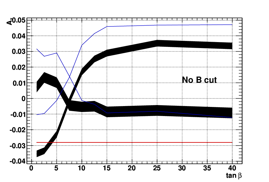
As before, one may compare the $H^{-}t$ and $Wt$ results. Here, though, a note of caution is necessary, because the difference between the DR and DS results for $Wt$ appears more pronounced for this parameter. In particular, it varies considerably before and after the boost cut is applied. This greater variation is perhaps exacerbated by the smallness of the asymmetry (which is at best only a few percent), but also suggests that interference with top pair production may be an issue in interpreting the $Wt$ results. It is nevertheless the case that the difference with $Wt$ is most pronounced at either low Higgs mass and high $\tan\beta$, or high Higgs mass and low $\tan\beta$. In both these cases, the sign of the top polarisation in $H^{-}t$ production is opposite to the one in $Wt$ production. This results in a small asymmetry of opposite sign to the $Wt$ case, but roughly comparable in size.

To summarise, we have here presented results for a number of angular and energy-related distributions and, building upon the analysis of [20, 23], defined a corresponding asymmetry parameter for each that efficiently encodes the difference in these distributions for different regions in the charged Higgs parameter space, as well as the differences between $Wt$ and $H^{-}t$ production. All of these asymmetries seem to be fairly robust against NLO and parton shower corrections. In addition, they complement each other, since different observables are sensitive to different parts of the parameter space. This suggests that they may indeed be very useful in isolating a charged Higgs boson, with subsequent identification of its properties. In the following section, we consider a second context in which such observables may be useful, namely that of isolating $Wt$ production itself as a signal.

4 Results for $Wt$ production

In the previous section, we examined the angular and energy distributions introduced in section 2 in $H^{-}t$ production, and defined asymmetry parameters which are potentially highly useful in elucidating the properties of a charged Higgs boson. In this section, we investigate whether these same observables have anything useful to say about Standard Model $Wt$ production.

There are three production modes for a single top quark in the Standard Model. Two of these, the so-called $s-$ and $t-$ channel modes, have been observed in combination at both the Tevatron [82, 83, 84] and LHC [85, 86]. The theoretical state of the art is also highly advanced, and includes fixed order computations [87, 88, 89, 90, 91], NLO plus parton shower implementations [92, 93], resummed results [94], and finite top width corrections [95, 96]. For related phenomenological studies, see [97, 98, 99, 100]. As already stated in the introduction, $Wt$ production offers a complementary window through which to look at top quark interactions, being sensitive to corrections to the $Wtb$ vertex, but not to four fermion operators which may affect the $s-$ and $t-$ channel modes. The investigation of $Wt$ production as a signal in its own right was first explored in [49]. Since then, computations have been carried out at NLO [51, 50], and also matched to a parton shower at this accuracy [52, 65].

The aim of this section is to examine angular observables and energy ratios for both $Wt$ and top pair production, for semi-realistic analysis cuts, and to reflect upon whether these results may be useful in enhancing the signal to background ratio of the former process. To this end, we adopt the following $Wt$ signal cuts, similar to those used in [53]:

$Wt$ signal cuts

1. The presence of exactly 1 $b$ jet with $p_{t}^{T}>50$ GeV and $|\eta|<2.5$. No other $b$ jets with $p_{t}^{T}>25$ GeV and $|\eta|<2.5$.

2. The presence of exactly 2 light flavor jets with $p_{t}^{T}>25$ GeV and $|\eta|<2.5$. In addition, their invariant mass should satisfy $55$ GeV$<m_{j_{1}j_{2}}<85$ GeV.

3. Events are vetoed if the invariant mass of the $b$ jet and light jet pair satisfies

   $$150\quad{\rm GeV}\quad<\sqrt{(p_{j_{1}}+p_{j_{2}}+p_{b})^{2}}\quad<\quad 190\quad{\rm GeV}.$$

4. The presence of exactly 1 isolated lepton with $p_{t}^{T}>25$ GeV and $|\eta|<2.5$. The lepton should satisfy $\Delta R>0.4$ with respect to the two light jets and the $b$ jet, where $R$ is the distance in the $(\eta,\phi)$ plane.

5. The missing transverse energy should satisfy $E^{miss}_{T}>$25 GeV.

Here the first cut is the most useful in getting rid of top pair production, as one expects two $b$ jets on average in $t\bar{t}$ production, but only one $b$ jet in $Wt$. The other cuts pick out semi-leptonic decays. That is, one $W$ boson decays to leptons (we would want this to be the $W$ boson from the top quark decay), and the other decays to quarks. We thus expect two light jets whose invariant mass reconstructs the $W$ mass, as well as a lepton and missing energy from the neutrino. The only difference with respect to the cuts used in [53] is the presence of an additional cut involving the invariant mass of the $b$ jet and light jet pair, restricting this to lie away from the top mass. This ensures that the selected semi-leptonic events are such that the top quark in $Wt$ decays leptonically, and the $W$ hadronically, as is required in order to use the decay lepton as a marker of top quark polarisation effects.

It was shown in [53] that, for these signal cuts (minus the invariant mass requirement for the three jets, which was unnecessary in that analysis), $Wt$ is a well-defined scattering process in that interference with pair production can be neglected. This was found by comparing the DR and DS results from MC@NLO. The results in this section were obtained using the DR subtraction method. Furthermore, the $Wt$ cross-section was found to be larger than the scale-variation uncertainty associated with the top pair cross-section. If this had not been true, then $Wt$ production would be swallowed up in the uncertainty of the top pair prediction, and much more care would be needed in order to be able to claim that it can be observed independently. We thus use the above cuts as an example of a fairly minimal analysis which guarantees that $Wt$ is a well-defined signal. We will see that even for this analysis, the angular and energy-related observables defined in section 2 display pronounced differences between $Wt$ and top pair production.

Note that in this section, in order to be more realistic, we consider distributions constructed from the isolated lepton entering the cuts. This is not guaranteed to be the decay lepton from the top quark, although the likelihood of this is increased by the event selection cuts. Also, we assume that the top quark direction is reconstructed with perfect resolution. In practice this would be done by considering the four-momenta of the $b$ jet and isolated lepton passing the cuts, together with missing energy. A full determination of the uncertainty induced in the reconstruction of the top quark (also including detector effects) is beyond the scope of the present study. Note that in $Wt$ and $W\bar{t}$ production, we assume that the top and antitop quark is reconstructed respectively. In top pair production, one constructs either the top or antitop quark which decays to give the isolated lepton passing the selection cuts. In contrast to the $H^{-}t$ results of the previous section, we present results for a centre of mass energy of 7 TeV. Jets are clustered using the $k_{T}$ algorithm [101] with D=0.7.

We first consider the azimuthal angle $\phi_{l}$, whose distribution is shown in figure 15 for both $Wt$ and top pair production.

Figure 15: Azimuthal angle distribution of the isolated lepton which enters the $Wt$ signal cuts, for both $Wt$ and top pair production, at NLO plus parton shower level.

The first thing to notice is that there is a distinct shape difference between the $Wt$ and top pair curves. The $Wt$ results include a slight peak structure at $\theta=\pi$, due to the contribution from events in which the $W$ boson decays leptonically, rather than the top quark. This structure is missing in the case of top pair production, due to the symmetrical nature of the final state. For the choice of analysis cuts given above, one may evaluate the asymmetry parameter $A_{\phi}$, which is shown in table 1.

$B_{cut}$	$Wt$	Top pair
0	0.33 $\pm$ 0.01	0.63 $\pm$ 0.02
0.8	0.41 $\pm$ 0.02	0.70 $\pm$ 0.05
0.9	0.42 $\pm$ 0.03	0.70 $\pm$ 0.07
0.95	0.44 $\pm$ 0.04	0.68 $\pm$ 0.08

Table 1: Results for the azimuthal asymmetry parameter $A_{\phi}$ of eq. (4), evaluated using the isolated lepton entering the $Wt$ selection cuts, and for different values of a cut $B>B_{cut}$ on the boost parameter of the top quark.

The values for $Wt$ and top pair production are significantly different. This is potentially a useful distinguishing feature between the two production processes.

Next, we consider the polar angle $\theta_{l}$, again defined in terms of the isolated lepton entering the $Wt$ signal cuts. The distribution of this angle is shown in figure 16.

Figure 16: Polar angle distribution of the isolated lepton which enters the $Wt$ signal cuts, for both $Wt$ and top pair production, at NLO plus parton shower level.

There is a notable difference between the $Wt$ and top pair production, due to the negative polarisation of the top in the former case. The corresponding asymmetry parameters $A_{\theta}$ are shown in table 2.

$B_{cut}$	$Wt$	Top pair
0	0.02 $\pm$ 0.01	0.26 $\pm$ 0.02
0.8	0.18 $\pm$ 0.02	0.38 $\pm$ 0.04
0.9	0.49 $\pm$ 0.03	0.75 $\pm$ 0.07
0.95	0.70 $\pm$ 0.05	0.97 $\pm$ 0.10

Table 2: Results for the polar asymmetry parameter $A_{\theta}$ of eq. (8), evaluated using the isolated lepton entering the $Wt$ selection cuts, and for different values of a cut $B>B_{cut}$ on the boost parameter of the top quark.

Again the results are different between the two production processes which, as in the azimuthal case, is a potentially useful discriminator between the two processes.

In the case of $H^{-}t$ production considered in section 3, we also considered various observables which depended upon the boost of the top quark. This is clearly of practical importance for heavy charged Higgs masses, which do indeed lead to heavily boosted top quarks in a sizeable fraction of events, as is clear from figure 1. One expects boosted top observables to be less useful in $Wt$ production, due to the fact that the $W$ boson is much lighter. Nevertheless, it is perhaps worth examining the dependence of various observables on the boost parameter of the top quark. If sizeable differences between $Wt$ and top pair production were to be observed, the impact on the signal to background ratio would then outweigh the loss in signal cross-section.

The distribution of the boost parameter $B$ of eq. (3) is shown for both $Wt$ and top pair production in figure 17, and one sees that there is a reasonable fraction of events in both cases which have $B>0.8$, albeit not as many as in the $H^{-}t$ case of the previous section. This is not surprising, given that charged Higgs masses of at least 200 GeV were considered there, so that the top recoiled against a much more massive particle than a $W$ boson. Here we also have a lower centre of mass energy. The $\phi_{l}$ distributions for the two processes are shown in figure 18 for different values of a cut $B>B_{cut}$.

Figure 17: Distribution of the boost parameter $B$ of eq. (3), at NLO plus parton shower level.

Figure 18: Azimuthal angle distribution of the isolated lepton which enters the $Wt$ signal cuts, for $Wt$ and top pair production, for different values of a cut $B>B_{cut}$ on the boost parameter of eq. (3), at NLO plus parton shower level.

One sees that, whilst there is some dependency on the boost parameter, the qualitative features remain identical. The corresponding asymmetries $A_{\phi}$ are given in table 1. One sees that the absolute value of the difference between the asymmetries for the two processes is roughly independent of the boost cut. However, the relative difference decreases.

One expects a much greater effect from the boost on the polar angle distribution, as the requirement of a boosted top will concentrate the decay products in polar angle. The $\theta_{l}$ distributions as a function of $B_{cut}$ are shown in figure 19.

Figure 19: Polar angle distribution of the isolated lepton which enters the $Wt$ signal cuts, for $Wt$ and top pair production, for different values of a cut $B>B_{cut}$ on the boost parameter of eq. (3), at NLO plus parton shower level.

The effect of the higher boost cut is to increase the peak region of the distribution at the expense of the tail, as expected. The corresponding $A_{\theta}$ values are collected in table 2. Unsurprisingly, both sets of results display an increase in $A_{\theta}$ as the boost cut is increased. This implies that a boost cut is actually detrimental in this case, as the relative difference between the asymmetry parameters in the two processes decreases.

Finally, we present results for the energy ratios of eqs. (5), which were shown to be useful for $H^{-}t$ production in section 3. In that case, we defined the energy of the $b$ quark via eq. (9), which is possible in a Monte Carlo study but not in a real experiment. Here, given that we have explicitly implemented analysis cuts in terms of jets, we define $E_{b}$ to be the energy of the $b$ jet which enters the cuts. Then the distributions of $z$ and $u$, with a cut on the boost parameter of $B>0.8$, are shown in figure 20.

Figure 20: Distributions of $u$ and $z$, as defined in eq. (5), where a cut on the boost parameter $B>0.8$ has been applied, at NLO plus parton shower level.

The first thing to note is that the results for the $u$ distribution do not show a significant difference between $Wt$ and top pair production. This is perhaps not so surprising given that we have already seen in section 3 that oppositely polarised top quarks tend to exhibit smaller differences in energy-related distributions than in angular distributions. Here we are essentially probing the difference between a polarised top quark and one which is unpolarised on average, and thus one expects an even smaller difference in behaviour.

The $z$ distribution in figure 20 shows some difference between the $Wt$ and top pair distributions. However, the top pair result does not closely resemble the flat profile one would expect for unpolarised top quarks, due presumably to that fact that the shape has been sculpted somewhat by the event selection cuts, in particular those which implement restrictions on jet invariant masses.

Given the above results, it does not seem particularly useful to examine the asymmetry parameters of eqs. (10, 11) in the present context. Nevertheless, the fact that a shape difference persists in the $z$ distribution between $Wt$ and top pair production still makes this a potentially useful observable in discriminating the two processes. One must also bear in mind the result for the polar asymmetry from above, namely that a boost cut will decrease the relative difference between the angular asymmetries in $Wt$ and top pair production. Thus, and perhaps unsurprisingly, the utility of boost cuts in $Wt$ production is somewhat limited.

5 Conclusion

In this paper, we have examined the role that observables which are sensitive to top quark polarisation can play in exploring the parameter space of charged Higgs models, and also in distinguishing $H^{-}t$ production from (Standard Model) $Wt$ production. In particular, we examined the azimuthal and polar angles $\phi_{l}$ and $\theta_{l}$ of [20, 23], and the energy ratios $z$ and $u$ of [15], defining corresponding asymmetry parameters analagous to that already defined for the azimuthal angle in [23]. Importantly, we found that polarisation effects are robust up to NLO and including parton shower corrections. At this level, each of the asymmetry parameters showed significant difference between different regions in the charged Higgs parameter space $(m_{H},\tan\beta)$, and also between $H^{-}t$ and $Wt$ production. The full set of asymmetries taken together thus provides a potentially highly useful probe of charged Higgs properties. Angular observables are sensitive only to corrections to the production of a top quark, and the polar angle is able to discriminate between charged Higgs masses at high $\tan\beta$ values, where the azimuthal angle cannot. Energy observables are sensitive to corrections to both the production and decay of top quarks. Although more difficult to construct (owing to the need for a cut on the boost parameter of the top quark), they give useful complementary information, particularly on the value of the charged Higgs mass at intermediate and high $\tan\beta$ values.

As a second application of these observables, we considered the problem of distinguishing Standard Model $Wt$ production from top pair production, which is a significant background. Under the assumption that it is meaningful to separate $Wt$ and top pair production, we observed significant differences, for semi-realistic $Wt$ analysis cuts, between angular distributions relating to the isolated lepton entering the cuts. It is worth pointing out that the cuts we used are fairly minimal in terms of signal to background ratio [53]. Nevertheless, large differences are obtained between the two production processes, which suggests that our findings would persist in a more realistic study, including detector effects etc.

One may also consider boosted top quark observables in Standard Model $Wt$ production, and we gave a couple of examples in section 4. These seem less useful than in $H^{-}t$ production, however. In the angular observables, a cut on the boost parameter does not increase the absolute difference between the asymmetry parameters for $Wt$ and top pair production, and decreases the relative difference. For energy observables, one sees only a small difference between the $u$ distributions even when a boost cut is applied. This is due mainly to the fact that one is comparing a polarised top quark in $Wt$ with an (on average) unpolarised top quark in top pair production, rather than an oppositely polarised top quark. A larger difference is observed in the $z$ distribution, which may yet be a useful observable in distinguishing $Wt$ and top pair production.

To summarise, the observables studied in this paper are useful probes of both $H^{-}t$ and $Wt$ production, and seem to be robust against higher order perturbative corrections. They therefore deserve further investigation.

References

- [1] R. Harlander, M. Jezabek, J. H. Kuhn, and T. Teubner, “Polarization in top quark pair production near threshold,” Phys.Lett. B346 (1995) 137–142, hep-ph/9411395.
- [2] K.-i. Hikasa, J. M. Yang, and B.-L. Young, “R-parity violation and top quark polarization at the Fermilab Tevatron collider,” Phys.Rev. D60 (1999) 114041, hep-ph/9908231.
- [3] S. D. Rindani and M. M. Tung, “Longitudinal quark polarization in e+ e- t anti-t and chromoelectric and chromomagnetic dipole couplings of the top quark,” Eur.Phys.J. C11 (1999) 485–493, hep-ph/9904319.
- [4] E. Boos, H. Martyn, G. A. Moortgat-Pick, M. Sachwitz, A. Sherstnev, et al., “Polarization in sfermion decays: Determining tan beta and trilinear couplings,” Eur.Phys.J. C30 (2003) 395–407, hep-ph/0303110.
- [5] T. Gajdosik, R. M. Godbole, and S. Kraml, “Fermion polarization in sfermion decays as a probe of CP phases in the MSSM,” JHEP 0409 (2004) 051, hep-ph/0405167.
- [6] B. C. Allanach, C. Grojean, P. Z. Skands, E. Accomando, G. Azuelos, et al., “Les Houches physics at TeV colliders 2005 beyond the standard model working group: Summary report,” hep-ph/0602198.
- [7] R. M. Godbole, S. Kraml, S. D. Rindani, and R. K. Singh, “Probing CP-violating Higgs contributions in through fermion polarization,” Phys.Rev. D74 (2006) 095006, hep-ph/0609113.
- [8] R. M. Godbole, S. D. Rindani, and R. K. Singh, “Lepton distribution as a probe of new physics in production and decay of the t quark and its polarization,” JHEP 12 (2006) 021, hep-ph/0605100.
- [9] P.-Y. Li, G.-R. Lu, J. M. Yang, and H. Zhang, “Probing R-parity Violating Interactions from Top Quark Polarization at LHC,” Eur.Phys.J. C51 (2007) 163–168, hep-ph/0608223.
- [10] M. Mohammadi Najafabadi, “Secondary particles spectra in decay of polarized top quark with anomalous tWb coupling,” J.Phys.G G34 (2007) 39–46, hep-ph/0601155.
- [11] P. Bhupal Dev, A. Djouadi, R. Godbole, M. Muhlleitner, and S. Rindani, “Determining the CP properties of the Higgs boson,” Phys.Rev.Lett. 100 (2008) 051801, 0707.2878.
- [12] D. Eriksson, G. Ingelman, J. Rathsman, and O. Stal, “New angles on top quark decay to a charged Higgs,” JHEP 01 (2008) 024, 0710.5906.
- [13] M. Perelstein and A. Weiler, “Polarized Tops from Stop Decays at the LHC,” JHEP 0903 (2009) 141, 0811.1024.
- [14] M. M. Nojiri and M. Takeuchi, “Study of the top reconstruction in top-partner events at the LHC,” JHEP 0810 (2008) 025, 0802.4142.
- [15] J. Shelton, “Polarized tops from new physics: signals and observables,” Phys. Rev. D79 (2009) 014032, 0811.0569.
- [16] R. M. Godbole, S. D. Rindani, K. Rao, and R. K. Singh, “Top polarization as a probe of new physics,” AIP Conf.Proc. 1200 (2010) 682–685, 0911.3622.
- [17] M. Arai, K. Huitu, S. K. Rai, and K. Rao, “Single production of sleptons with polarized tops at the Large Hadron Collider,” JHEP 1008 (2010) 082, 1003.4708.
- [18] A. Djouadi, G. Moreau, F. Richard, and R. K. Singh, “The Forward-backward asymmetry of top quark production at the Tevatron in warped extra dimensional models,” Phys.Rev. D82 (2010) 071702, 0906.0604.
- [19] D. Krohn, J. Shelton, and L.-T. Wang, “Measuring the Polarization of Boosted Hadronic Tops,” JHEP 07 (2010) 041, 0909.3855.
- [20] R. M. Godbole, K. Rao, S. D. Rindani, and R. K. Singh, “On measurement of top polarization as a probe of production mechanisms at the LHC,” JHEP 11 (2010) 144, 1010.1458.
- [21] J. A. Aguilar-Saavedra and J. Bernabeu, “W polarisation beyond helicity fractions in top quark decays,” Nucl. Phys. B840 (2010) 349–378, 1005.5382.
- [22] C. Degrande, J.-M. Gerard, C. Grojean, F. Maltoni, and G. Servant, “Non-resonant New Physics in Top Pair Production at Hadron Colliders,” JHEP 1103 (2011) 125, 1010.6304.
- [23] K. Huitu, S. Kumar Rai, K. Rao, S. D. Rindani, and P. Sharma, “Probing top charged-Higgs production using top polarization at the Large Hadron Collider,” JHEP 04 (2011) 026, 1012.0527.
- [24] J. Cao, L. Wu, and J. M. Yang, “New physics effects on top quark spin correlation and polarization at the LHC: a comparative study in different models,” Phys.Rev. D83 (2011) 034024, 1011.5564.
- [25] D.-W. Jung, P. Ko, and J. S. Lee, “Longitudinal top polarization as a probe of a possible origin of forward-backward asymmetry of the top quark at the Tevatron,” Phys.Lett. B701 (2011) 248–254, 1011.5976.
- [26] D. Choudhury, R. M. Godbole, S. D. Rindani, and P. Saha, “Top polarization, forward-backward asymmetry and new physics,” Phys.Rev. D84 (2011) 014023, 1012.4750.
- [27] S. Gopalakrishna, T. Han, I. Lewis, Z.-g. Si, and Y.-F. Zhou, “Chiral Couplings of W’ and Top Quark Polarization at the LHC,” Phys.Rev. D82 (2010) 115020, 1008.3508.
- [28] R. Godbole, C. Hangst, M. Muhlleitner, S. Rindani, and P. Sharma, “Model-independent analysis of Higgs spin and CP properties in the process ,” Eur.Phys.J. C71 (2011) 1681, 1103.5404.
- [29] D. Krohn, T. Liu, J. Shelton, and L.-T. Wang, “A Polarized View of the Top Asymmetry,” 1105.3743.
- [30] M. Baumgart and B. Tweedie, “Discriminating Top-Antitop Resonances using Azimuthal Decay Correlations,” JHEP 1109 (2011) 049, 1104.2043.
- [31] S. D. Rindani and P. Sharma, “Probing anomalous tbW couplings in single-top production using top polarization at the Large Hadron Collider,” 1107.2597.
- [32] J. Baglio, M. Beccaria, A. Djouadi, G. Macorini, E. Mirabella, et al., “The Left-Right asymmetry of top quarks in associated top-charged Higgs bosons at the LHC as a probe of the tan parameter,” 1109.2420.
- [33] S. D. Rindani and P. Sharma, “CP violation in tbW couplings at the LHC,” 1108.4165.
- [34] B. Ananthanarayan, M. Patra, and S. D. Rindani, “Top-spin analysis of new scalar and tensor interactions in collisions with beam polarization,” Phys.Rev. D83 (2011) 016010, 1007.5183.
- [35] K. Agashe, A. Belyaev, T. Krupovnickas, G. Perez, and J. Virzi, “LHC Signals from Warped Extra Dimensions,” Phys.Rev. D77 (2008) 015003, hep-ph/0612015.
- [36] A. Falkowski, G. Perez, and M. Schmaltz, “Spinning the Top,” 1110.3796.
- [37] M. Jezabek and J. H. Kuhn, “Lepton Spectra from Heavy Quark Decay,” Nucl.Phys. B320 (1989) 20.
- [38] A. Czarnecki, M. Jezabek, and J. H. Kuhn, “Lepton spectra from decays of polarized top quarks,” Nucl.Phys. B351 (1991) 70–80.
- [39] A. Brandenburg, Z. Si, and P. Uwer, “QCD corrected spin analyzing power of jets in decays of polarized top quarks,” Phys.Lett. B539 (2002) 235–241, hep-ph/0205023.
- [40] B. Grzadkowski and Z. Hioki, “New hints for testing anomalous top quark interactions at future linear colliders,” Phys.Lett. B476 (2000) 87–94, hep-ph/9911505.
- [41] B. Grzadkowski and Z. Hioki, “Decoupling of anomalous top decay vertices in angular distribution of secondary particles,” Phys.Lett. B557 (2003) 55–59, hep-ph/0208079.
- [42] B. Grzadkowski and Z. Hioki, “Angular distribution of leptons in general production and decay,” Phys.Lett. B529 (2002) 82–86, hep-ph/0112361.
- [43] Z. Hioki, “A New decoupling theorem in top quark physics,” in Seogwipo 2002, Linear colliders, pp. 333–338. 2002. hep-ph/0210224.
- [44] K. Ohkuma, “Effects of top quark anomalous decay couplings at gamma gamma colliders,” Nucl.Phys.Proc.Suppl. 111 (2002) 285–287, hep-ph/0202126.
- [45] S. D. Rindani, “Effect of anomalous t b W vertex on decay lepton distributions in e+ e- t anti-t and CP violating asymmetries,” Pramana 54 (2000) 791–812, hep-ph/0002006.
- [46] R. M. Godbole, S. D. Rindani, and R. K. Singh, “Study of CP property of the Higgs at a photon collider using gamma gamma t anti-t lX,” Phys.Rev. D67 (2003) 095009, hep-ph/0211136.
- [47] ATLAS Collaboration, “ATLAS Public Note no. ATL-PHYS-PUB-2010-008,” 2010.
- [48] C. Weydert et al., “Charged Higgs boson production in association with a top quark in MC@NLO,” Eur. Phys. J. C67 (2010) 617–636, 0912.3430.
- [49] T. M. P. Tait, “The mode of single top production,” Phys. Rev. D61 (2000) 034001, hep-ph/9909352.
- [50] J. M. Campbell and F. Tramontano, “Next-to-leading order corrections to W t production and decay,” Nucl. Phys. B726 (2005) 109–130, hep-ph/0506289.
- [51] S. Zhu, “Next-to-leading order QCD corrections to b g t W- at the CERN Large Hadron Collider,” Phys. Lett. B524 (2002) 283–288.
- [52] S. Frixione, E. Laenen, P. Motylinski, B. R. Webber, and C. D. White, “Single-top hadroproduction in association with a W boson,” JHEP 07 (2008) 029, 0805.3067.
- [53] C. D. White, S. Frixione, E. Laenen, and F. Maltoni, “Isolating Wt production at the LHC,” JHEP 11 (2009) 074, 0908.0631.
- [54] W. Bernreuther, “Top quark physics at the LHC,” J.Phys.G G35 (2008) 083001, 0805.1333.
- [55] J. Alwall, M. Herquet, F. Maltoni, O. Mattelaer, and T. Stelzer, “MadGraph 5 : Going Beyond,” JHEP 1106 (2011) 128, 1106.0522.
- [56] J. Alwall, P. Demin, S. de Visscher, R. Frederix, M. Herquet, et al., “MadGraph/MadEvent v4: The New Web Generation,” JHEP 0709 (2007) 028, 0706.2334.
- [57] S. Frixione and B. R. Webber, “Matching NLO QCD computations and parton shower simulations,” JHEP 0206 (2002) 029, hep-ph/0204244.
- [58] S. Frixione and B. R. Webber, “The MC@NLO 3.4 Event Generator,” 0812.0770.
- [59] S. Frixione, F. Stoeckli, P. Torrielli, B. R. Webber, and C. D. White, “The MC@NLO 4.0 Event Generator,” 1010.0819.
- [60] S. Frixione, P. Nason, and B. R. Webber, “Matching NLO QCD and parton showers in heavy flavor production,” JHEP 0308 (2003) 007, hep-ph/0305252.
- [61] S. Frixione, E. Laenen, P. Motylinski, and B. R. Webber, “Angular correlations of lepton pairs from vector boson and top quark decays in Monte Carlo simulations,” JHEP 04 (2007) 081, hep-ph/0702198.
- [62] S. Frixione, P. Nason, and C. Oleari, “Matching NLO QCD computations with Parton Shower simulations: the POWHEG method,” JHEP 0711 (2007) 070, 0709.2092.
- [63] W. T. Giele, D. A. Kosower, and P. Z. Skands, “A Simple shower and matching algorithm,” Phys.Rev. D78 (2008) 014026, 0707.3652.
- [64] S. Frixione, P. Nason, and G. Ridolfi, “A Positive-weight next-to-leading-order Monte Carlo for heavy flavour hadroproduction,” JHEP 0709 (2007) 126, 0707.3088.
- [65] E. Re, “Single-top Wt-channel production matched with parton showers using the POWHEG method,” Eur.Phys.J. C71 (2011) 1547, 1009.2450.
- [66] C. Weydert, “Associated production of top quarks and charged Higgs bosons at next-to-leading order,” IL NUOVO CIMENTO 33 C (2010) 1011.6249.
- [67] N. Kauer and D. Zeppenfeld, “Finite width effects in top quark production at hadron colliders,” Phys. Rev. D65 (2002) 014021, hep-ph/0107181.
- [68] B. P. Kersevan and I. Hinchliffe, “A consistent prescription for the production involving massive quarks in hadron collisions,” JHEP 09 (2006) 033, hep-ph/0603068.
- [69] A. Denner, S. Dittmaier, S. Kallweit, and S. Pozzorini, “NLO QCD corrections to WWbb production at hadron colliders,” Phys.Rev.Lett. 106 (2011) 052001, 1012.3975.
- [70] G. Bevilacqua, M. Czakon, A. van Hameren, C. G. Papadopoulos, and M. Worek, “Complete off-shell effects in top quark pair hadroproduction with leptonic decay at next-to-leading order,” JHEP 1102 (2011) 083, 1012.4230.
- [71] W. Beenakker, R. Hopker, M. Spira, and P. Zerwas, “Squark and gluino production at hadron colliders,” Nucl.Phys. B492 (1997) 51–103, hep-ph/9610490.
- [72] T. Plehn, “Production of supersymmetric particles at high-energy colliders,” hep-ph/9809319. Ph.D. Thesis.
- [73] T. Plehn and C. Weydert, “Charged Higgs production with a top in MC@NLO,” in PoS CHARGED2010, p. 026. 2010. 1012.3761.
- [74] T. Binoth, D. Goncalves-Netto, D. Lopez-Val, K. Mawatari, T. Plehn, et al., “Automized Squark-Neutralino Production to Next-to-Leading Order,” 1108.1250.
- [75] A. Djouadi, “The Anatomy of electro-weak symmetry breaking. I: The Higgs boson in the standard model,” Phys. Rept. 457 (2008) 1–216, hep-ph/0503172.
- [76] A. Djouadi, “The Anatomy of electro-weak symmetry breaking. II. The Higgs bosons in the minimal supersymmetric model,” Phys. Rept. 459 (2008) 1–241, hep-ph/0503173.
- [77] UTfit Collaboration, M. Bona et al., “An Improved Standard Model Prediction Of BR(B -¿ tau nu) And Its Implications For New Physics,” Phys. Lett. B687 (2010) 61–69, 0908.3470.
- [78] A. D. Martin, W. J. Stirling, R. S. Thorne, and G. Watt, “Parton distributions for the LHC,” Eur. Phys. J. C63 (2009) 189–285, 0901.0002.
- [79] A. D. Martin, W. J. Stirling, R. S. Thorne, and G. Watt, “Uncertainties on in global PDF analyses and implications for predicted hadronic cross sections,” Eur. Phys. J. C64 (2009) 653–680, 0905.3531.
- [80] A. D. Martin, W. J. Stirling, R. S. Thorne, and G. Watt, “Heavy-quark mass dependence in global PDF analyses and 3- and 4-flavour parton distributions,” Eur. Phys. J. C70 (2010) 51–72, 1007.2624.
- [81] A. Djouadi, J. Kalinowski, and M. Spira, “HDECAY: A program for Higgs boson decays in the standard model and its supersymmetric extension,” Comput. Phys. Commun. 108 (1998) 56–74, hep-ph/9704448.
- [82] CDF Collaboration, T. Aaltonen et al., “First Observation of Electroweak Single Top Quark Production,” Phys.Rev.Lett. 103 (2009) 092002, 0903.0885.
- [83] D0 Collaboration, V. M. Abazov et al., “Observation of Single Top-Quark Production,” Phys. Rev. Lett. 103 (2009) 092001, 0903.0850.
- [84] D0 Collaboration, V. M. Abazov et al., “Model-independent measurement of -channel single top quark production in collisions at TeV,” Phys.Lett. B705 (2011) 313–319, 1105.2788.
- [85] CMS Collaboration, S. Chatrchyan et al., “Measurement of the t-channel single top quark production cross section in pp collisions at sqrt(s) = 7 TeV,” Phys. Rev. Lett. 107 (2011) 091802, 1106.3052.
- [86] R. Schwienhorst and f. t. A. collaboration, “Single top-quark production with the ATLAS detector in pp collisions at sqrt(s)=7TeV,” 1110.2192.
- [87] B. W. Harris, E. Laenen, L. Phaf, Z. Sullivan, and S. Weinzierl, “The fully differential single top quark cross section in next-to-leading order QCD,” Phys. Rev. D66 (2002) 054024, hep-ph/0207055.
- [88] J. M. Campbell, R. K. Ellis, and F. Tramontano, “Single top production and decay at next-to-leading order,” Phys. Rev. D70 (2004) 094012, hep-ph/0408158.
- [89] Q.-H. Cao and C. P. Yuan, “Single top quark production and decay at next-to-leading order in hadron collision,” Phys. Rev. D71 (2005) 054022, hep-ph/0408180.
- [90] Q.-H. Cao, R. Schwienhorst, and C. P. Yuan, “Next-to-leading order corrections to single top quark production and decay at Tevatron. I: s-channel process,” Phys. Rev. D71 (2005) 054023, hep-ph/0409040.
- [91] Q.-H. Cao, R. Schwienhorst, J. A. Benitez, R. Brock, and C. P. Yuan, “Next-to-leading order corrections to single top quark production and decay at the Tevatron. II: t-channel process,” Phys. Rev. D72 (2005) 094027, hep-ph/0504230.
- [92] S. Frixione, E. Laenen, P. Motylinski, and B. R. Webber, “Single-top production in MC@NLO,” JHEP 03 (2006) 092, hep-ph/0512250.
- [93] S. Alioli, P. Nason, C. Oleari, and E. Re, “NLO single-top production matched with shower in POWHEG: s- and t-channel contributions,” JHEP 09 (2009) 111, 0907.4076.
- [94] N. Kidonakis, “Next-to-next-to-leading-order collinear and soft gluon corrections for t-channel single top quark production,” Phys.Rev. D83 (2011) 091503, 1103.2792.
- [95] P. Falgari, F. Giannuzzi, P. Mellor, and A. Signer, “Off-shell effects for t-channel and s-channel single-top production at NLO in QCD,” Phys.Rev. D83 (2011) 094013, 1102.5267.
- [96] P. Falgari, P. Mellor, and A. Signer, “Production-decay interferences at NLO in QCD for -channel single-top production,” Phys.Rev. D82 (2010) 054028, 1007.0893.
- [97] Q.-H. Cao, J. Wudka, and C. P. Yuan, “Search for New Physics via Single Top Production at the LHC,” Phys. Lett. B658 (2007) 50–56, 0704.2809.
- [98] Z. Sullivan, “Angular correlations in single-top-quark and W j j production at next-to-leading order,” Phys. Rev. D72 (2005) 094034, hep-ph/0510224.
- [99] Z. Sullivan, “Understanding single-top-quark production and jets at hadron colliders,” Phys. Rev. D70 (2004) 114012, hep-ph/0408049.
- [100] P. Motylinski, “Angular correlations in t-channel single top production at the LHC,” Phys. Rev. D80 (2009) 074015, 0905.4754.
- [101] S. Catani, Y. L. Dokshitzer, M. Seymour, and B. Webber, “Longitudinally invariant clustering algorithms for hadron hadron collisions,” Nucl.Phys. B406 (1993) 187–224.