Temperature-Dependent Behavior of Confined Many-electron Systems in the Hartree-Fock Approximation

Abstract

Many-electron systems confined at substantial finite temperatures and densities present a major challenge to density functional theory. Comparatively little is known about the free-energy behavior of such systems for temperatures and pressures of interest, for example, in the study of warm dense matter. As a result, development of approximate free-energy functionals is faced with difficulties of assessment and calibration. Here we address, in part, this need for detailed results on well-characterized systems. We present results on a comparatively simple, well-defined, but computationally feasible model, namely the thermal Hartree-Fock approximation applied to eight one-electron atoms with nuclei at fixed, arbitrary positions in a hard-walled box. We discuss the main technical tasks (defining a suitable basis and evaluation of the required matrix elements) and discuss the physics which emerges from the calculations.

I Introduction

Warm dense matter (WDM) is encountered in systems as diverse as the interiors of giant planets [1, 2] and in the pathway to inertial confinement fusion [3, 4]. WDM is challenging to theory and simulation because it occurs inconveniently, for theory, between the comparatively well-studied plasma and condensed matter regimes. Both the Coulomb coupling parameter $\Gamma:=Q^{2}/(r_{s}k_{B}{\rm T})$ and electron degeneracy parameter $\Theta:=k_{B}{\rm T}/\varepsilon_{F}$ are approximately unity for WDM. ($Q=$ relevant charge, $r_{s}=$ Wigner radius, $\varepsilon_{F}=$ electron Fermi energy, ${\rm T}=$ temperature, $k_{B}=$ Boltzmann constant.) A non-perturbative treatment therefore is required.

Contemporary computations on WDM [5, 6, 7, 8, 9, 10, 11, 12, 13, 14, 15, 16, 17, 18] are dominated by use of the Kohn-Sham (KS) realization of thermal density functional theory (DFT) [19, 20, 21, 22, 23, 24, 25] to generate a potential surface for ionic motion (treated classically). The great majority of these calculations use approximate ground-state exchange-correlation (XC) functionals, $E_{xc}$, with the temperature dependence of the XC free energy picked up implicitly from the $\rm T$-dependence of the density $n({\mathbf{r}},{\rm T})$. Though fruitful, this approach is not without potential difficulties, as is illustrated in Fig. 3 of Ref. 7. Three issues are germane here.

First, virtually nothing systematic is known about the implicit $\rm T$-dependence of ground-state approximate $E_{xc}$ functionals (especially beyond the local density approximation, LDA), whether they be constraint-based or empirical. Compared to the ground-state situation, there is only a small literature on explicitly $\rm T$-dependent functionals, that is, XC free energy functionals, and essentially all of those studies are at the level of the LDA [26, 27, 28, 29, 30, 31, 32, 33, 34, 35, 36, 37, 38, 39, 40, 41, 42].

Second, there is the computational burden of solving for the Kohn-Sham orbitals and eigenvalues. Since the computational load from the eigenvalue problem scales, in general, as order $N_{\rm orbitals}^{3}$, the growth in the number of non-negligibly occupied KS orbitals with increasing temperature is a clear computational bottleneck. See the remarks, for example, in Sec. 4 of Ref. 18. For complicated systems, the same bottleneck is encountered in ground-state simulations which use the DFT Born-Oppenheimer energy surface to drive the ionic dynamics. One result has been the emergence of active research on orbital-free DFT (OFDFT), that is, approximate functionals for the ingredients of the KS free energy, namely the KS kinetic energy (KE) ${\mathcal{T}}_{s}$, entropy ${\mathcal{S}}_{s}$, and XC free energy $\mathcal{F}_{xc}$ or their ground-state counterparts. Almost all of this effort has been for ground-state OFKE functionals [43, 44, 45, 46]. (Note that most of the OFKE literature invokes the KS separation of the KE in order to use existing $E_{xc}$ approximations consistently.)

Third, the finite-temperature OFDFT work is dominated by variants on Thomas-Fermi-von Weizsäcker theory; see for example Ref. 41 and references therein. That type of theory, however, is known (on both fundamental and computational grounds) to be no more than qualitatively accurate in many circumstances relevant to WDM (e.g., chemical binding). Compared to the data-rich context for development of zero-temperature functionals, there is little to guide development and assessment of finite-T functionals. Similarly, compared to the T=0 situation (or the very high T situation), not much is known about the accuracy of approximate finite-T OFDFT functionals beyond TFvW. An aim of the present study is to provide such data for the combination of a well-defined physical system with a well-defined approximation and its implementation.

II System and Methodology

We shall treat a neutral system of $N_{ion}$ atoms with nuclei fixed at arbitrary positions in a hard-walled three-dimensional rectangular box. The confined system allows systematic treatment of pressure effects at stipulated finite temperature, hence is a small, treatable sample of WDM. For specificity in the initial work, we chose one-electron atoms and $N_{ion}\leq 8$ for simplicity. Note the corresponding use of a small number of atoms in Ref. 18. Also note the considerable literature on spherically confined systems at ${\rm T}=0$ K [47, 48, 49, 50, 51, 52]. We have not found any work on lower-symmetry confinement of multi-atom systems at non-zero $\rm T$. At non-zero $\rm T$ there is a large literature on average-atom methods, for example Refs. 53, 18 and many others, but such methods do not provide the fiduciary data needed for functional development.

As a many-electron problem, a clearly defined approximation is required. We choose the finite temperature Hartree-Fock (FTHF) scheme [23, 54, 55, 56], with issues of electron correlation to be addressed in the future. FTHF provides a clear definition for the correlation free energy which is consistent with the definition used in zero-temperature theory with approximate wave functions. (Of course, the definition of correlation energy in zero-temperature DFT differs, as it does in finite-temperature DFT, but that is no more a barrier here than there.) In addition to being well-defined in the grand ensemble, FTHF provides the advantage that its ${\rm T}=0$ K limit is the lingua franca of molecular electronic structure interpretation. Use of FTHF therefore also provides at least a semi-quantitative framework for understanding chemical processes in WDM.

The FTHF approximation is defined in the grand canonical ensemble by restricting the relevant traces to states which are single Slater determinants [23, 54, 55]. The result is an upper bound to the free energy $\mathcal{F}_{FTHF}\geq\mathcal{F}$. Standard thermodynamic relationships for the grand ensemble follow. The FTHF Euler equations to be solved (in unrestricted form) are [55]

$$\varepsilon_{i}\varphi_{i}(\mathbf{r})= \left(-\frac{1}{2}\nabla^{2}+U_{ion}(\mathbf{r})\right)\varphi_{i}(\mathbf{r})$$

$$+\sum_{j}{f_{j}\int{d\mathbf{r^{\prime}}\frac{\left|\varphi_{j}(\mathbf{r^{\prime}})\right|^{2}}{\left|\mathbf{r}-\mathbf{r^{\prime}}\right|}}\varphi_{i}(\mathbf{r})}$$

$$-\sum_{j}{\delta_{\sigma_{i}\sigma_{j}}f_{j}\int{d\mathbf{r^{\prime}}\frac{\varphi_{j}^{*}(\mathbf{r^{\prime}})\varphi_{i}(\mathbf{r^{\prime}})}{\left|\mathbf{r}-\mathbf{r^{\prime}}\right|}}\varphi_{j}(\mathbf{r})}\,,$$ (1)

with $U_{ion}$ the ion-electron interaction potential and $\sigma_{i}$ the spin label; the sums are over all spin orbitals. Unless indicated otherwise we use hartree atomic units ($\hbar=m_{e}=e=1$; energy is then in hartrees, l hartree = 27.2116 eV, and lengths are in bohrs, 1 bohr = 0.52918 angstrom). The spin orbitals (eigenstates, $\varphi_{i}$) have Fermi-Dirac thermal occupations

$$f_{i}=\left(1+e^{\beta(\varepsilon_{i}-\mu)}\right)^{-1}\;,\quad N=\sum_{i}f_{i}\;,$$ (2)

where $\beta=1/k_{B}{\rm T}$ and $\mu$ is the electron chemical potential. For a specified value of $N$, which is a grand ensemble average, $\mu$ must be determined. These equations, along with specification of the nuclear sites and imposition of hard-wall boundary conditions, completely describe the problem.

The FTHF free energy and entropy are given by

$$\mathcal{F}_{FTHF}=\sum_{i}{f_{i}\varepsilon_{i}}-\frac{1}{2}\sum_{i,j}f_{i}f_{j}\left(J_{i,j}-K_{i,j}\right)-{\rm T}{\mathcal{S}_{FTHF}}\;,$$ (3)

$$\mathcal{S}_{FTHF}=-k_{B}\sum_{i}{f_{i}\ln(f_{i})+(1-f_{i})\ln(1-f_{i})}\;,$$ (4)

with conventional definitions of $J$ and $K$:

$$J_{i,j}:= \int d\mathbf{r}d\mathbf{r^{\prime}}\frac{\left|\varphi_{i}(\mathbf{r})\right|^{2}\left|\varphi_{j}(\mathbf{r^{\prime}})\right|^{2}}{\left|\mathbf{r}-\mathbf{r^{\prime}}\right|}\;,$$ (5)

$$K_{i,j}:= \delta_{\sigma_{i}\sigma_{j}}\int d\mathbf{r}d\mathbf{r^{\prime}}\frac{\varphi_{i}(\mathbf{r})\varphi_{j}(\mathbf{r})\varphi_{i}^{*}(\mathbf{r^{\prime}})\varphi_{j}^{*}(\mathbf{r^{\prime}})}{\left|\mathbf{r}-\mathbf{r^{\prime}}\right|}\;.$$ (6)

Equations (3) and (4) clearly reduce to conventional ground-state Hartree-Fock expressions in the zero-temperature limit.

II.1 Gaussian Basis Sets

Solution of self-consistent field equations such as (1) via Gaussian-type-orbital (GTO) basis methods is the standard procedure in modern computational codes for molecular systems. First introduced by Boys [61, 62, 63, 64, 65], such basis sets automatically satisfy the free-molecule boundary condition that the orbitals vanish at infinity. For a hard-wall confined system, the basis functions must vanish at the boundary, so standard molecular GTO matrix-element expressions are inapplicable. This fact illustrates the most critical technical issue for implementation, namely, to find a basis that satisfies the boundary conditions yet allows for an efficient enough evaluation of the two-electron integrals to be computationally tractable on reasonable resources. A second, closely related technical issue is that the high temperature also dictates what is “efficient enough”, in that the basis must be large enough and flexible enough to represent a sufficient number of thermally occupied higher-energy orbitals of the system, hence to represent the density and free energy accurately.

Those considerations eliminate several seemingly plausible options for a basis. For example, a real-space finite-difference/element scheme, while suitable for a DFT calculation or a Hartree-Fock calculation on a free diatomic molecule (for which curvilinear coordinates can be exploited [57]), is far too expensive for the present case because of the number of matrix elements to be calculated. Another example is sine functions. They also satisfy the hard-wall boundary condition, but an adequate description of the rapidly varying electronic distribution near the nuclei requires prohibitively many matrix elements in our multi-center problems. So we chose an adaptation of standard GTO methods which uses modified Gaussians that meet the boundary condition, yet retain enough efficiency to complete the calculation.

The various ways to force a GTO to zero at the bounding planes of a rectangular box can have great impact upon the efficiency of the matrix element calculations. Compared with familiar practice for free molecules, in general the confined case requires more primitive GTOs for each contracted one. More importantly, the finite integration volume makes it impossible to achieve completely analytic calculation of the two-electron integrals, which is, of course, precisely the category in which computational efficiency is most needed. We have addressed this issue by using truncated Gaussians as described in the next section.

II.2 Truncated Gaussians

The rectangular box makes Cartesian GTOs a convenient choice, because each primitive function then is separable into Cartesian factors which are simple 1D functions. Consider the Cartesian factor

$$g^{n}(x)=(x-x_{c})^{n}e^{-\alpha(x-x_{c})^{2}}$$ (7)

To force this function to zero at the box boundaries $x=0$ and $x=L_{x}$, we subtract a constant equal to the function value at each end. When $x_{c}$ is not at the box center, the value to be subtracted differs for the two ends, so we split the function into two pieces, make the two subtractions, and scale the two pieces such that the resulting function is continuous. Each unnormalized Cartesian factor becomes

$$g^{n}_{box}(x) =a_{0}\left(g^{n}(x)-\Delta_{0}\right)\quad 0\leq x\leq x_{c}$$

$$=a_{L}\left(g^{n}(x)-\Delta_{L_{x}}\right)\quad x_{c}\leq x\leq L_{x}$$ (8)

with $\Delta_{0}=g^{n}(0)$, $\Delta_{L_{x}}=g^{n}(L_{x})$. We call this the truncated GTO (tGTO) basis.

Two technical issues remain. The tGTO functions may not have continuous derivatives, so proper evaluation of the kinetic energy matrix elements requires attention. Appendix A shows that nothing untoward happens and that the kinetic energy is simply a sum of piecewise contributions, except for $p$-type functions which have a simple correction term. Second is the matter of evaluating two-electron matrix elements. In Appendix B, we show that this task reduces to computing finite-range integrals of products of Gaussians and error functions. At this juncture, we are doing those via Gauss-Legendre quadrature. We also note that the tGTO basis is simpler than the smoothly cut-off floating spherical GTO basis of Ref. 51 in the sense that their cut-off introduces a mixing of two symmetry types (e.g. s, d) in each basis function.

Note that, so far, we have implemented only the restricted Hartree-Fock approximation (RHF; non-spin-polarized in DFT language; closed-shell or spin-compensated in quantum chemistry language).

III Results

III.1 Zero Temperature

Two simple ground-state test cases, the H atom and the H₂ molecule, illustrate the system behavior with increasing confinement (decreasing volume) as well as the correctness of our implementation. The confined-system energies should be above the ground-state energies (in the basis selected) of the corresponding free systems and approach those free-system energies (and bond length for the molecule) in the limit of large box volume.

For the hydrogen atom in the center of a cubical box, Fig. 1 (a) shows the ground-state energy for confinements $L\leq 10$ bohr. (The basis exponents shown in Table 1; their selection is described in the next section.) The calculations were carried out to $L=30$ bohr. Beyond $10$ bohr there was negligible difference in the energy with respect to the free-atom energy in the same basis, precisely as expected. At $L=30$ bohr the ground-state energy is identical with the free-atom GTO calculation using the same basis, namely $-0.498476$ hartree, validating our overlap, kinetic, and nuclear energy integral calculations. A fit to the energies as a function of cube edge $L$

$$E(L)=a/L^{2}+b/L+c\;\;,\quad 0\leq L\leq 10\,\,\mathrm{bohr}$$ (9)

yields $a=14.5733$ hartree bohr², $b=-3.82369$, hartree bohr, $c=-0.238258$ hartree. Though this fit does not have the correct infinite-size limit, it is the best fit of this simple form for $0\leq L\leq 10$ bohr. ¿From this fit the pressure, $p=-dE/dV$ ($V=L^{3}$) can be calculated; see Fig. 1 (b).

Figure 1: (a) Ground-state energy of an H atom in the center of a cube with edge length $L$. Fit is for function $f(L)=a/L^{2}+b/L+c$. (b) Pressure calculated from the energy fit.

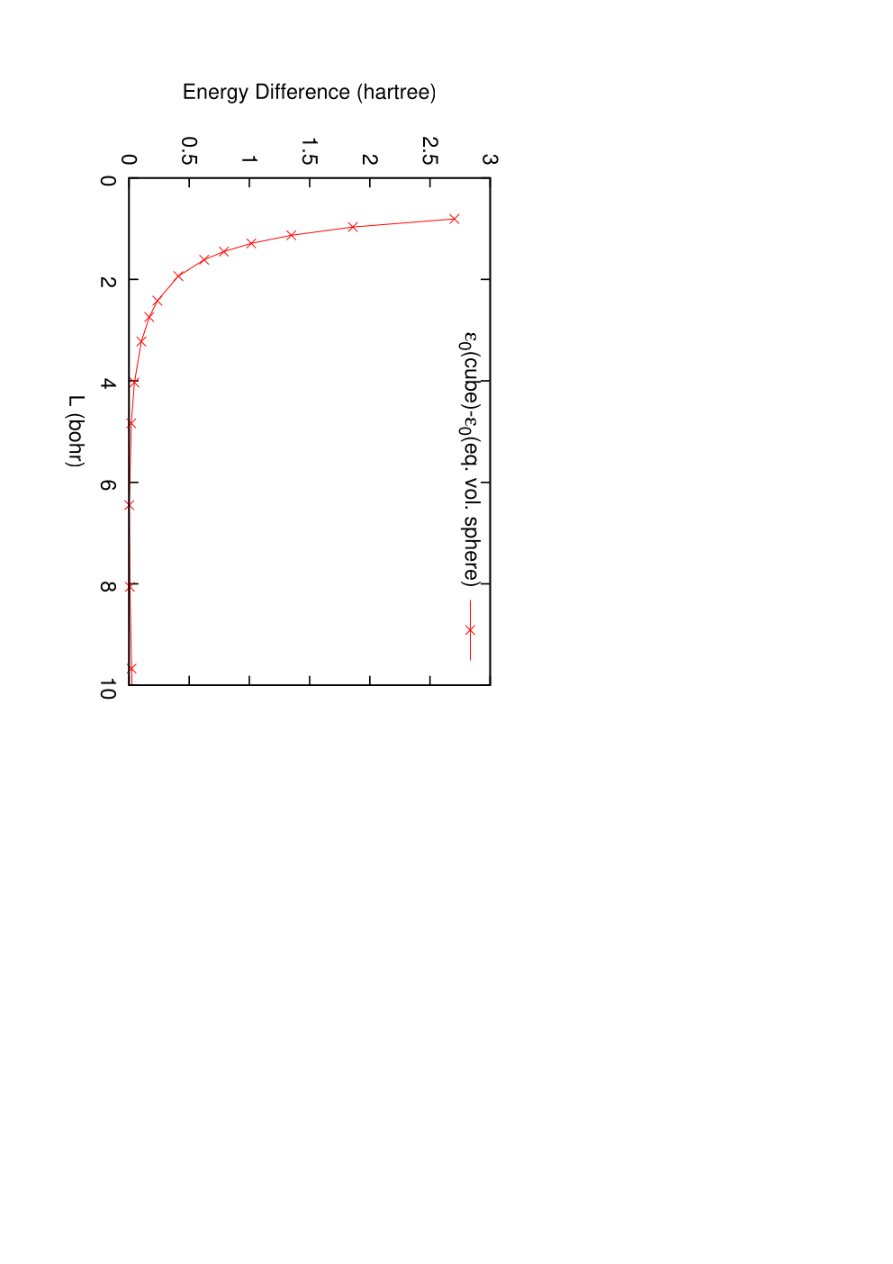
The effects of spherical versus cubic confinement can be assessed easily by comparison of the two confinement types both for bounding volumes and equal volumes. For bounding volumes, the circumscribed-sphere $R=\sqrt{3}L/2$ and inscribed-sphere $R=L/2$ results from Ref. 59 (also see Ref. 58) can be compared to our cube results. Figure 2 shows that the energy of the cubically confined system is bounded by that of the two spherical systems, as expected. Shape effects of confinement are shown in Fig. 3. Though the spherical system has a lower energy than that of the equal volume cubical system, they are quite close until the cube is smaller than $L\approx 4$ bohr, where a significant indication of shape dependence begins. At $L=1$ bohr the difference in energy is over $25\%$, as shown in Fig. 3 (b). A simpler basis of six $s$-type tGTO with exponents [0.15,0.3,0.6,1.2,2.4,4.8 bohr^-2] reproduces the ground-state energies for $L\geq 1.5$ bohr.

Figure 2: Comparison of ground-state energy of an H atom in a cube with its energy within two bounding spheres.

Figure 3: (a) Comparison of energy of an H atom in a cube with that in a sphere of equal volume. (b) The difference of the two ground-state energies.

Next consider the confined H₂ molecule at zero temperature. Here we used the simpler six-tGTO basis just given. For a large cube, the new tGTO confined-box computations again should conform to known results for the integrals and produce essentially the energy vs. bond length curve for the free molecule. With $L=30$ bohr and the molecule centered in the cube and aligned along the body diagonal, we get energies shown as points in Fig. 4. These agree completely with the values of the free GTO calculation, which are shown in that figure as the “Free” curve. The minimum is at 1.383 bohr, satisfactorily close to the free-molecule RHF value of 1.385 bohr from a 6-31G^∗∗ basis calculation [60].

Figure 4: Energy versus atomic separation for the H₂ molecule centered in a 30 bohr cube. The ground-state agrees exactly with the free GTO calculation using the same primitives as a basis.

Conversely for fixed $\mathrm{R}$ (at 1.4 bohr) and decreasing $L$ (to 4 bohr), the ground-state energy behavior is shown in Fig. 5.

Figure 5: Ground-state energy for H₂ with bond length $1.4$ bohr confined in cube of edge length $L$.

The onset of confinement effects becomes visible in the vicinity of $L\approx 11$ bohr. Optimization of the bond length $\mathrm{R}$ at $L=5$ bohr is shown in Fig. 6. The total energy is, of course, higher than for the larger box, and the optimal $\mathrm{R}$ is shifted down to $1.178$ bohr from $1.383$ bohr.

Following this method, we obtain the optimized $\mathrm{R}$ and energy for decreasing $L$. A function fit to the energy similar to that used earlier yields $\mathrm{R}$ as a function of the pressure, as shown in Fig. 7.

Figure 6: Energy vs. bond length for the H₂ molecule centered in cubes $L=30$ and $L=5$ bohr. The minima are at $1.383$ and $1.178$ bohr respectively.

Figure 7: Optimized bond length, $\mathrm{R}$, for the H₂ molecule vs. pressure.

III.2 Finite Temperature

For finite-temperature calculations, at least a single p orbital needs to be included, and as many orbitals as feasible should be available to represent the fractionally occupied levels which become increasingly important as $\rm T$ is increased. For all the following calculations, except where noted, the basis consists of seven s-type primitive GTOs and one $p_{x}$, one $p_{y}$, and one $p_{z}$ GTO, with the $p$-GTO exponents equal. An elementary exponent optimization was done as follows. A set of five $s$-type exponents was picked and held fixed: [0.1,0.2,0.4,0.8,1.6 bohr^-2]. The sixth exponent was optimized to to minimize $\varepsilon_{1s}$ for the single atom centered in a cube of specified $L$. With those six exponents fixed, the seventh $s$-GTO exponent was used to minimize $\varepsilon_{2s}$. With those seven fixed, the $p$ exponent was used to minimize $\varepsilon_{2p}$. Additionally, for small $L$ the smallest exponents produce orbitals that are so similarly flat that an approximate linear dependence exists and diagonalization fails. When this happens the smallest exponent is replaced by extending the even-tempered exponent series to larger values. For example at $L=4$ the $0.1$ exponent is replaced with $3.2$, at $L=2$ the $0.2$ exponent is also replaced with $6.4$.

This procedure keeps the ratio of the effective length ($1/\sqrt{\alpha}$) of the most diffuse function to the edge length $L$ at 0.75-0.79 for $L\leq 3$, with smaller ratios for larger $L$.

The optimization was done for each $L$. Table 1 shows the resulting exponents and energies for the orbitals that were optimized.

L	fixed	1$s$	2$s$	2$p$	$\varepsilon_{1s}$	$\varepsilon_{2s}$	$\varepsilon_{2p}$
1.0	1.6, 3.2, 6.4, 12.8, 25.6	179.1	244 (NA)	4.01	10.518	50.5898	26.683
1.5	0.8, 1.6, 3.2, 6.4, 12.8	92.15	244 (NA)	1.88	3.6738	21.3545	11.154
2	0.4, 0.8, 1.6, 3.4, 6.8	48	250	1.115	1.48471	11.3649	5.8753
3	0.2, 0.4, 0.8, 1.6, 3.4	24.5	175	0.545	0.11385	4.47073	2.25356
4	0.2, 0.4, 0.8, 1.6, 3.4	21.2	7.0	0.34	$-$0.268848	2.18313	1.06314
5	0.1, 0.2, 0.4, 0.8, 1.6	11.2	3.7	0.235	$-$0.40474	1.18372	0.547955
6	”	10.4	2.5	0.18	$-$0.458898	0.675591	0.288794
7	”	17.7	2.25	0.15	$-$0.481704	0.389716	0.145105
8	”	10.2	0.195	0.122	$-$0.491112	0.217062	0.0591604
9	”	10.2	0.07	0.103	$-$0.495291	0.10651	0.00450443
10	”	10.2	0.0365	0.088	$-$0.497104	0.0327616	$-$0.0321549
11	”	10.1	0.023	0.076	$-$0.497889	$-$0.0179536	$-$0.0578267
12	”	10.1	0.018	0.0665	$-$0.498227	$-$0.0535872	$-$0.0764093
13	”	10.1	0.015	0.059	$-$0.498372	$-$0.0789901	$-$0.0901715
14	”	10.05	0.014	0.053	$-$0.498435	$-$0.0972631	$-$0.100500
15	”	10.1	0.014	0.048	$-$0.498461	$-$0.108291	$-$0.108291

Table 1: Optimized exponents and orbital energies for an H atom at the center of a cube of edge length $L$. 2$p$ refers to the triply degenerate $p_{x}$, $p_{y}$, and $p_{z}$ states. For $L<2$, the 2$s$ level could not be optimized beyond the first 6 exponents.

With this volume-dependent optimized basis, calculations were done for a single atom at the center of a cube with $1\leq L\leq 15$ bohr. The orbital energies of the five lowest states (1$s$, 2$p_{x}$, 2$p_{y}$, 2$p_{z}$, 2$s$) are plotted in Fig. 8. Notice the inversion of ordering ($2p$ below $2s$) that is a result primarily of the confinement.

Figure 8: Lowest five eigenstate energies of H as a function of cube edge $L$. Energy values are from Table 1.

To address finite temperature for this single-electron system, the one-electron levels were populated according to the Fermi-Dirac distribution. Observe that the one-electron Hamiltonian is independent of density, so the one-electron orbitals and eigen-energies are independent of occupancy, even though the density and total electronic energy are not. The left-hand panel in Fig. 9 shows the resulting total energy as a function of $L$ for four values of $\rm T$, while the right-hand panel shows the free energy. The weak minimum in total energy in the vicinity of $6$ bohr at T=50 kK appears to be a confinement effect. We have found a similar minimum at about the same volume by doing a Fermi-Dirac population of the high-precision eigenvalues of the spherically confined H atom given in Ref. 59.

Figure 9: (a) Single H atom total energy, $E={\mathcal{F}}_{FTHF}+{\rm T}{\mathcal{S}}_{FTHF}$, and (b) free energy, $\mathcal{F}_{FTHF}$ as a function of cube edge $L$, with the one-electron levels populated according to the Fermi distribution.

Figure 10: Energy components of a cubically confined single H atom vs. temperature.  (a) kinetic energy, (b) electron-nuclear energy, (c) total energy, (d) free energy, (e) entropic energy [(d)-(c)]. Key for all is shown in (e).

Figure 10 shows the contributions to the free energy for the single atom as a function of $\rm T$ for four cube volumes ($L=$ 2, 3, 7, 15 bohr). At $L=7$ bohr, the KE is flat with $\rm T$ at almost its $\rm T=0$ K value. The $\rm T=50$ kK nuclear-electron attraction $E_{Ne}$, however, is much stronger for $L=7$ bohr than for $L=15$ bohr. By $L=3$ bohr, the KE and $E_{Ne}$ are roughly equal in magnitude.

Figure 10 also shows that the KE for the $L=15$ bohr system falls with increasing temperature. Though this might seem odd, it is as it should be from virial theorem arguments for the free atom. The 2$s$ KE is one-fourth the 1$s$ value [66]. Finite temperature population of the 2$s$ and depopulation of the 1$s$ therefore reduces the KE with respect to its $\rm T=0$ K value.

Next we turn to the system of eight H atoms. We examined a symmetric configuration in which the eight atoms were situated at the corners of a smaller cube, edge-length $L/2$, centered within the hard-wall cube, edge-length $L$. The basis used was ten s-type GTOs centered on each atom. Strict s-type symmetry is broken, of course, by enforcement of the hard-wall boundary conditions. An even-tempered set of exponents also was used in this case: [0.2,0.4,0.8,1.6,3.2,6.4,12.8,25.2,50.4,100.8 bohr^-2]. As a test, the calculations were redone with two fewer basis functions per atom; the exponents [50.4,100.8 bohr^-2] were removed. The two calculations agreed to 2 millihartree in total and component energies up to 200 kK. Matrix elements are calculated only once and stored, after which fully self-consistent calculations may be done at many temperatures.

Figure 11: Zero and finite-temperature total energy and free energy for eight H atoms in different sized cubes: (a) $E={\mathcal{F}}_{FTHF}+{\rm T}{\mathcal{S}}_{FTHF}$, (b) $\mathcal{F}_{FTHF}$.

Figure 12: Self-consistent FTHF free energy contributions for eight confined H atoms in a cubic array as a function of $\rm T$ for four different cube edge lengths $L$. Key for all is given in (d).

Figure 11 shows the total energy $E={\mathcal{F}}_{FTHF}+{\rm T}{\mathcal{S}}_{FTHF}$ as a function of $L$ for various temperatures, as well as the free energy $\mathcal{F}_{FTHF}$ itself. The nuclear-nuclear repulsion energy is included (constant with respect to temperature, it varies with $L$). Figure 12 shows various components of the free energy (electron-nuclear Coulomb energy, electron-electron Coulomb energy including exchange, kinetic energy, and entropic energy). Also shown are the total energy and free energy, with the difference of these two being the entropic energy. Again, the nuclear-nuclear repulsion energy is included in these two plots. It has values of 9.118, 7.598, 5.699, 4.559 hartree for $L=$ 5, 6, 8, 10 bohr, respectively. The energies are shown as a function of temperature $0\leq{\mathrm{T}}\leq 250$kK for four cube sizes, $L=$ 5, 6, 8, and 10 bohr. The comparatively flat plateau up to roughly ${\mathrm{T}}=15$ kK is a direct consequence of Fermi-Dirac level filling. Up to about 25 kK, the interval between the highest occupied molecular orbital (HOMO) at zero temperature and the lowest unoccupied molecular orbital (LUMO) is roughly constant at 0.5 hartree. Therefore the filling ratio of those two is roughly $\exp(-13/1.3)\approx 5\times 10^{-5}$ or smaller up to about ${\mathrm{T}}=15$kK. We return to this matter below.

III.3 Comparison with approximate functionals

Orbital-free treatment of WDM has been dominated, not surprisingly, by local density approximations for both the KE and exchange contributions to the free energy. For the KE, the choice is physically motivated by the fact that the high-pressure and/or high-temperature limit for a WDM system is Thomas-Fermi. This leads to finite-temperature Thomas-Fermi (FTTF) [67] ${\mathcal{T}}_{0}=\int\tau_{0}\;d\mathbf{r}$ by itself, or with some fraction of von Weizsäcker contribution (in its zero-temperature form) ${\mathcal{T}}_{W}=\int\tau_{W}\;d\mathbf{r}$, with

$$\tau_{0} =\frac{\sqrt{2}}{\pi^{2}\beta^{5/2}}I_{3/2}(\beta\mu)$$ (10)

$$n =\frac{\sqrt{2}}{\pi^{2}\beta^{3/2}}I_{1/2}(\beta\mu)$$ (11)

$$\tau_{W} =\frac{\left|\nabla n\right|^{2}}{8n}$$ (12)

where the $I$ are Fermi integrals. Note a parametrized form [26] may be used to eliminate $\mu$ between $\tau_{0}$ and $n$.

In Fig. 13 we compare the FTHF KE as a function of $\mathrm{T}$ with the FTTF KE alone and with it supplemented by both the full ${\mathcal{T}}_{W}$ and $(1/9){\mathcal{T}}_{W}$ for $L=6$ bohr. The latter three functionals were evaluated with the FTHF density, hence are non-self-consistent. As is known at ${\mathrm{T}}=0$, pure Thomas-Fermi underestimates the KE while addition of the full ${\mathcal{T}}_{W}$ overestimates it. None of the three is close to quantitative agreement with ${\mathcal{T}}_{FTHF}$. Moreover, FTTF and FTTF augmented with $(1/9){\mathcal{T}}_{W}$ can be ruled out from the ${\mathrm{T}}=0$ K comparison, since the exact (fully correlated) KE must be above ${\mathcal{T}}_{FTHF}$ (from a virial theorem argument).

Figure 13: FTHF kinetic energy compared with finite-temperature Thomas-Fermi KE and two forms of von Weizsäcker augmentation of FTTF for $L=6$ bohr. See text for details.

For the exchange contribution to the free energy, the use of ground-state functionals is common (recall Introduction), with the LDA being dominant. Fig. 14 shows the FTHF exchange contribution to the free energy ${\mathcal{F}}_{x,FTHF}$ in comparison with the exchange free-energy generated by ground-state LDA functional and with the Perrot and Dharma-wardana parametrization for the temperature-dependent LDA functional [28]. Again, this is for $L=6$ bohr and the other functionals are evaluated with the FTHF density. (Note that such “post-scf” evaluation is fairly common in assessment of newly developed ground state functionals. See, for example, Ref. 68.) Here one sees a marked difference: the ground-state functional fails completely while the temperature-dependent functional has at least semi-quantitatively correct temperature dependence.

Figure 14: FTHF exchange free energy ground-state LDA and Perrot and Dharma-wardana temperature-dependent LDA ($L=6$ bohr). See text for details.

We may also make some semi-quantitative comparison with a more widely used model for extended systems at substantial T. In Fig. 15 we show the internal energy per atom of the eight hydrogen atoms in the cubic symmetry arrangement at $L=7$ bohr (corresponds to average $r_{s}=2.17$), with that of the average atom DFT calculation of Dharma-wardana and Perrot [70] at $r_{s}=2$. Their system includes DFT exchange and correlation whereas we have pure Hartree-Fock exchange. Additional energy differnces are due to the different boundary conditions. Decomposing the near parallel temperature dependence into those components, however, is a task outside the scope of the present work. We can already see one aspect. Though the kinetic energy is the major contributor to the change in total energy as a function of temperature (recall Fig. 12), the change due to electron-electron interaction, including exchange, is at least a third that of the kinetic energy.

Figure 15: FTHF internal energy per atom for $L=7$ bohr, as compared with $r_{s}=2$ hydrogen plasma average atom DFT calculation.

IV Discussion and Conclusions

Comparison, evaluation, and betterment of functionals for WDM simulations is the long-term motive of this work. As just shown, even at this initial state of development (Hartree-Fock, small particle number, no molecular dynamics), the approach gives insight regarding that task. There are some specific issues worth discussion also.

IV.1 One-particle spectrum effects

It is well known that zero-temperature HF calculations over-estimate both band gaps in solids and the so-called HOMO-LUMO (highest occupied and lowest empty molecular orbital respectively) gaps of finite systems. This happens because the occupied HF orbitals are free of self-interaction, but the unoccupied ones are not. As temperature increases in the FTHF scheme, however, levels unoccupied at T = 0 K become increasingly occupied and shifted. In the self-consistent solution of the HF problem in a basis, those levels then contribute to the Hamiltonian matrix (“Fock matrix” in quantum chemistry terminology). Thus there are two questions to address. What is the extent to which FTHF exhibits HOMO-LUMO gap over-estimation similar to that of ground-state HF? At what fractional occupancy is an energy level changed from an overestimated virtual to a more properly estimated partially occupied one?

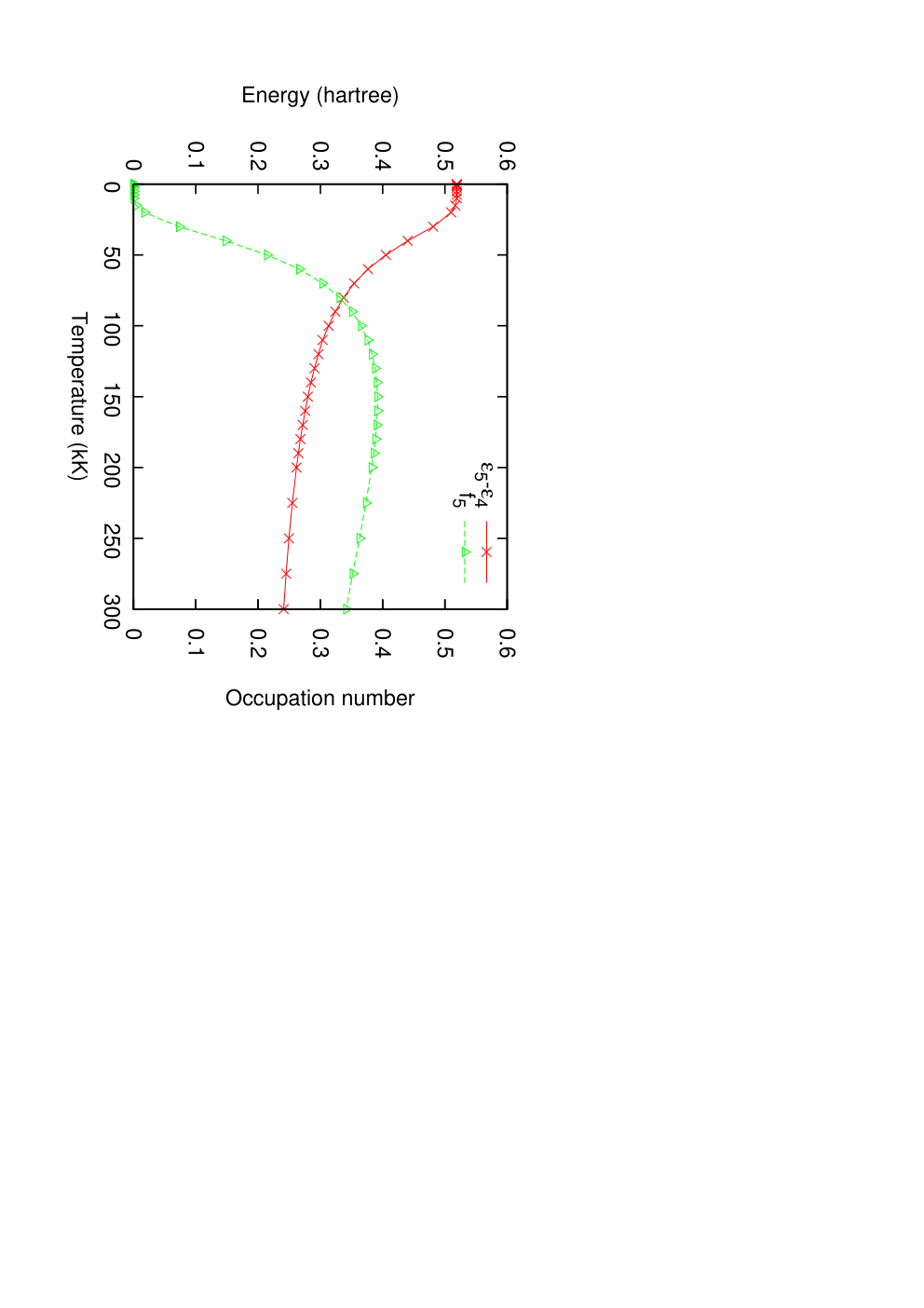
For specificity, we consider the eigenspectrum of a single, moderately compressed eight-atom cube with $L=6$ bohr. Figure 16 shows the Fermi distribution of the single-particle energies for four temperatures. Note that these distributions are for one spin. Also keep in mind that the cubical symmetry causes the lowest four one-electron orbitals to group as singly degenerate and triply degenerate (a1g, t1u in crystal field notation). At zero temperature therefore, only two points are shown with unit occupancy, but the higher energy point corresponds to three degenerate HOMO states (indexed as 2, 3, 4). The LUMO is the degenerate states 5, 6, and 7, with the singly degenerate state 8 above them (again as would be expected from a cubical crystal field). For simplicity of discussion, the HOMO and LUMO (at ${\rm T}=0$) are labeled $\varepsilon_{4}$ and $\varepsilon_{5}$ respectively. One can see that the spacing between $\varepsilon_{4}$ and $\varepsilon_{5}$ decreases with temperature. This difference is shown directly in Fig. 18 along with the occupation number for the $\varepsilon_{5}$ level. The continuous curves in Fig. 16 show the Fermi function with calculated chemical potential $\mu$. The discrete points mark the input energies to the calculation of $\mu$. Then in Fig. 17, $\mu$ is plotted as a function of $\rm T$. Observe that the chemical potential is nearly mid-way between $\varepsilon_{4}$ and $\varepsilon_{5}$ up to just below $50$ kK. This behavior is exact at zero temperature.

Those total energy and eigenspectrum results together resolve the matter of the behavior of what would be virtual states at zero temperature in FTHF. First, examination of the kinetic and total energy plots for all box sizes shows that there is a change in the form of the temperature dependence at roughly $20$ kK. That change is complemented by the change in the spacing between the $\varepsilon_{4}$ and $\varepsilon_{5}$ levels. They are essentially static for lower temperatures, then begin to change abruptly well below $50$ kK, and then change more moderately at higher temperatures. Thus, above $50$ kK, states corresponding to zero-temperature virtuals are sufficiently incorporated in the interaction terms to make a material modification of ${\rm T}=0$ behavior. However, as the temperature is decreased below roughly $50$ kK, the FTHF Coulomb and exchange terms increasingly are dominated by the ${\rm T}=0$ occupied levels, which therefore keeps the lightly occupied higher energy levels artificially high. This is not a basis issue, but an issue with discrete eigenstates. In a solid such as jellium or a metal with a continuum of states, this should not be an issue, but for a system with energy gaps the issue remains.

Figure 16: Fermi distribution for eight H atoms in a box of size $L=6$ bohr. Points may represent more than one state due to energy degeneracies.

Figure 17: Chemical potential $\mu$ and the fourth and fifth energy levels. The curve labeled “middle” is half way between $\varepsilon_{4}$ and $\varepsilon_{5}$.

Figure 18: Energy difference between the fourth and fifth energy levels along with the occupation number of the fifth energy level.

IV.2 Other findings and considerations

The preceding discussion about depopulation and repopulation of levels relative to the ground-state HF HOMO-LUMO gap illustrates a broader challenge for the construction of approximate functionals for the various contributions to the free energy. Whether explicit or implicit, such approximate functionals correspond to restricting the required traces to specific classes (or sub-sets of classes) of state functions. The consequence of such a restriction is to incorportate the spectral properties of that class into the approximate functionals. For example, in FTHF that class is single Slater determinants constructed with respect to ground-state HF minimization. Although we have not attempted its construction here, in principle there is an FTHF free-energy functional. It would have exactly the same problem with a plateau in its T-dependence as we have found here.

The small number of particles is another issue. For sufficiently large numbers, all standard ensembles (grand canonical, canonical, micro-canonical) give the same thermodynamics. Fluctuations characteristic of small particle counts can degrade that relationship. Such issues are endemic to any computational study, especially when a large temperature and pressure domain such as characterizes WDM is involved. In that sense, the present study is not much worse off than most modern WDM simulations with small numbers of electrons [69]. At the least, we have an even-handed comparison of different methods (e.g., the comparison of functionals given above) for a given number of electrons and of ions. The main issue regarding particle count is computational cost.

Clearly we have shown that the tGTO basis is feasible and effective. As is typical of GTO basis methods, the computational cost is essentially entirely in the cpu time for the calculation of the two-electron integrals. The eight-atom systems described are calculated with 64 or 80 total basis functions, making diagonalization trivial. A simple double array of all $N^{4}$ two-electron integrals only occupies 128 or 312.5 MB respectively, storable in memory. In practice we calculated $N^{4}/\lambda$ integrals, with $\lambda=$7.60, 7.68 and not 8 due to the looping procedure we used. While for the cubic system discussed here, this calculation requirement could have been reduced further by exploiting symmetry, we need the capability to explore other, lower symmetry geometries. Note however that if the box size or the atomic positions are changed, all integrals affected by the change must be recalculated.

On a modern desktop processor (Intel Core i5 650 at 3.2 Ghz) one two-electron integral can be calculated in about 29.1 ms. So the times to calculate all integrals for a 64- or 80-orbital basis would be 17.84 hr and 43.13 hr. The integrals are calculated independently, so can be parallelized effectively. Calculations reported in this work were done on the University of Florida High Performance Computing Center Linux clusters.

Though these are quite acceptable costs for fixed geometries and small numbers of ions and electrons, the burden becomes formidable for direct application in Born-Oppenheimer molecular dynamics. We are currently working on ways to ameliorate that problem.

V Acknowledgement

This work was supported under US DOE Grant DE-SC0002139. We acknowledge useful conversations with Mike Murillo early in this work and continuing discussions with our colleagues Jim Dufty, Keith Runge, and Valentin Karasiev. We also thank the University of Florida High Performance Computing Center for computational support.

Appendix A Correction for Piecewise Integrals for the Basis Functions

From the definition of the basis functions in Eqs. (7) and (8), it follows that derivatives of the basis function may not be continuous at $x_{c}$, the center of the function. A discontinuity of the second derivative would, of course, be significant for the kinetic energy. The issue is whether the kinetic energy matrix elements can be evaluated piecewise, as is the case with the overlap, nuclear-electron, and electron-electron integrals. We may examine this issue by writing the basis formally with Heaviside functions, as follows:

$$\varphi=\left[\theta(x)-\theta(x-x_{1})\right]\varphi_{0}+\left[\theta(x-x_{1})-\theta(x-L)\right]\varphi_{L}$$ (13)

For the tGTO basis, the identification from Eq. 8 is

$$\varphi_{0}=a_{0}\left(g^{n}(x)-\delta_{0}\right)$$

$$\varphi_{L}=a_{L}\left(g^{n}(x)-\delta_{L}\right)$$

$$g^{n}(x)=(x-x_{1})^{n}e^{-\alpha(x-x_{1})^{2}}\;,\quad x_{1}=x_{c}\;$$ (14)

The derivatives are

$$\frac{\partial\varphi}{\partial x}= \left[\delta(x)-\delta(x-x_{1})\right]\varphi_{0}+\left[\theta(x)-\theta(x-x_{1})\right]\varphi_{0}^{\prime}$$

$$+\left[\delta(x-x_{1})-\delta(x-L)\right]\varphi_{L}$$

$$+\left[\theta(x-x_{1})-\theta(x-L)\right]\varphi_{L}^{\prime}$$ (15)

and

$$\frac{\partial^{2}\varphi}{\partial x^{2}}= \left[\delta^{\prime}(x)-\delta^{\prime}(x-x_{1})\right]\varphi_{0}+2\left[\delta(x)-\delta(x-x_{1})\right]\varphi_{0}^{\prime}$$

$$+\left[\theta(x)-\theta(x-x_{1})\right]\varphi_{0}^{\prime\prime}$$

$$+\left[\delta^{\prime}(x-x_{1})-\delta^{\prime}(x-L)\right]\varphi_{L}$$

$$+2\left[\delta(x-x_{1})-\delta(x-L)\right]\varphi_{L}^{\prime}$$

$$+\left[\theta(x-x_{1})-\theta(x-L)\right]\varphi_{L}^{\prime\prime}\;$$ (16)

Now consider a generic kinetic energy matrix element involving the foregoing function and another, similar basis function $\chi$ with left and right constituents $\chi_{0}$, $\chi_{L}$, centered at $x_{2}$. Without loss of generality, take $x_{1}<x_{2}$. Then

$$\int_{0}^{L}\chi\frac{\partial^{2}\varphi}{\partial x^{2}}\;dx:=I_{A}+I_{B}$$ (17)

The terms of the second derivative with the Heaviside functions contribute just the piecewise integration $I_{A}$, while the delta function and first derivative delta function terms contribute $I_{B}$. Of the terms in Eq. 16 only those at $x_{1}$ contribute, as the constituents $\chi_{0}$, $\chi_{L}$, $\varphi_{0}$, and $\varphi_{L}$ go to zero at $x=0$ and $x=L$. Thus

$$I_{B}= \int\chi_{0}\left[\delta^{\prime}(x-x_{1})\left(\varphi_{L}-\varphi_{0}\right)\right.$$

$$\left.+2\delta(x-x_{1})\left(\varphi_{L}^{\prime}-\varphi_{0}^{\prime}\right)\right]\;dx\;.$$ (18)

From the definition of $\delta^{\prime}$ this expression becomes

$$I_{B}= \int\chi_{0}\left[-\delta(x-x_{1})\left(\varphi_{L}^{\prime}-\varphi_{0}^{\prime}\right)\right.$$

$$\left.+2\delta(x-x_{1})\left(\varphi_{L}^{\prime}-\varphi_{0}^{\prime}\right)\right]-\chi_{0}^{\prime}\delta(x-x_{1})\left(\varphi_{L}-\varphi_{0}\right)\;dx\;\;$$ (19)

which reduces to

$$I_{B}=\left[\chi_{0}\left(\varphi_{L}^{\prime}-\varphi_{0}^{\prime}\right)-\chi_{0}^{\prime}\left(\varphi_{L}-\varphi_{0}\right)\right]\bigg|_{x=x_{1}}\;$$ (20)

For the case of $x_{1}=x_{2}$, that is, for diagonal terms or functions that have the same center, $\chi_{0}^{\prime}$ must be replaced in Eq. (19) by the analog of Eq. (15), with the result

$$I_{B}=\chi_{0}\left(\varphi_{L}^{\prime}-\varphi_{0}^{\prime}\right)\bigg|_{x=x_{1}}-\int \delta(x-x_{1})\left(\varphi_{L}-\varphi_{0}\right)\left[\left[\delta(x)-\delta(x-x_{1})\right]\chi_{0}+\left[\theta(x)-\theta(x-x_{1})\right]\chi_{0}^{\prime}\right.$$

$$+\left.\left[\delta(x-x_{1})-\delta(x-L)\right]\chi_{L}+\left[\theta(x-x_{1})-\theta(x-L)\right]\chi_{L}^{\prime}\right]\;dx\;$$ (21)

Note $\chi_{0}$ in the first term follows because the functions themselves are continuous,while the first and second derivatives may not be. For the same reason, it follows that the remaining integral in Eq. (21) and the second term of Eq. (20) vanish. Thus so long as the functions are continuous, the correction to the piecewise kinetic energy integral is simply

$$I_{B}=\chi(\varphi_{L}^{\prime}-\varphi_{0}^{\prime})\bigg|_{x=x_{1}}$$ (22)

and so long as the first derivative is continuous, this reduces to zero.

With continuity of the basis functions enforced by construction, only the first derivative needs to be examined for a possible correction to simple piecewise integration. For the basis defined in Eqs. (8), those corrections are

$$g^{0}(x) =e^{-\alpha(x-x_{1})^{2}} I_{B}=0$$

$$g^{1}(x) =(x-x_{1})e^{-\alpha(x-x_{1})^{2}} I_{B}=\chi(a_{L}-a_{0})$$

$$g^{2}(x) =(x-x_{1})^{2}e^{-\alpha(x-x_{1})^{2}} I_{B}=0\;$$ (23)

Basis functions $g^{n}(x)$ with higher powers of the prefactor $(x-x_{1})$ all have continuous first and second derivatives at $x_{1}$. In fact, those derivatives are all zero. So only the $p$-type basis functions, $(n=1)$, have a kinetic energy matrix element contribution beyond that given by piecewise integration.

Appendix B Finite-Range Gaussian Integrals

Following the methods of Boys [61, 62, 63, 64, 65], we use the transform of the Coulomb potential to separate the Coulomb integrals into one-dimensional Cartesian pieces:

$$\frac{1}{\left|{\bf r}-{\bf R_{N}}\right|}=\frac{1}{\sqrt{\pi}}\int_{-\infty}^{\infty}e^{-s^{2}({\bf r}-{\bf R_{N}})^{2}}ds$$

$$=\frac{1}{\sqrt{\pi}}\int_{-\infty}^{\infty}e^{-s^{2}(x-X_{N})^{2}}e^{-s^{2}(y-Y_{N})^{2}}e^{-s^{2}(z-Z_{N})^{2}}ds\;.$$ (24)

Hence all Coulomb integrals require integration over the transform variable $s$, which is done by Gauss-Laguerre quadrature.

For 1D primitive tGTOs, we note the required finite range $(a,b)$ integrals are of the form

$$I_{n}=\int_{a}^{b}x^{n}e^{-\alpha(x-x_{c})^{2}}\;dx$$ (25)

This simply transforms to

$$I_{n}=\int_{a-x_{c}}^{b-x_{c}}(x^{\prime}+x_{c})^{n}e^{-\alpha x^{\prime 2}}\;dx^{\prime}$$ (26)

This result leaves us needing to compute

$$J_{n}=\int_{a^{\prime}}^{b^{\prime}}x^{n}e^{-\alpha x^{2}}\;dx$$ (27)

Integrating by parts we find

$$J_{n}=-x^{n-1}\frac{e^{-\alpha x^{2}}}{2\alpha}\bigg|_{a^{\prime}}^{b^{\prime}}+\frac{n-1}{2\alpha}J_{n-2}$$ (28)

So with the initial two integrals, we may find the higher-order integrals by recursion:

$$J_{0} =\int_{a^{\prime}}^{b^{\prime}}e^{-\alpha x^{2}}\;dx=\frac{\sqrt{\pi}}{2\sqrt{\alpha}}\erf\left(\sqrt{\alpha}x\right)\bigg|_{a^{\prime}}^{b^{\prime}}$$ (29)

$$J_{1} =\int_{a^{\prime}}^{b^{\prime}}xe^{-\alpha x^{2}}\;dx=-\frac{e^{-\alpha x^{2}}}{2\alpha}\bigg|_{a^{\prime}}^{b^{\prime}}$$ (30)

All two-center (overlap, nuclear-electron, kinetic) integrals reduce to expressions in terms of $I_{n}$. After two applications of the Gaussian product rule, four-center (two-electron) integrals reduce to terms of the form

$$\int_{a_{2}}^{b_{2}}\int_{a_{1}}^{b_{1}}x_{1}^{n}x_{2}^{m}e^{-\alpha_{1}(x_{1}-x_{i})^{2}}e^{-\alpha_{2}(x_{2}-x_{j})^{2}}e^{-s^{2}(x_{1}-x_{2})^{2}}\;dx_{1}dx_{2}$$ (31)

Two further applications of the product rule bring us to the form

$$\int_{a_{2}}^{b_{2}}\int_{a_{1}}^{b_{1}}x_{1}^{n}x_{2}^{m}e^{-\kappa_{1}(x_{1}-R_{1}(x_{2}))^{2}}e^{-\kappa_{2}(x_{2}-R_{2})^{2}}\;dx_{1}dx_{2}$$ (32)

Here the integral over $x_{1}$ may be evaluated as $I_{n}$, so we are left with

$$\int_{a_{2}}^{b_{2}}I_{n}(x_{2})\bigg|_{x_{1}=a_{1}}^{x_{1}=b_{1}}x_{2}^{m}e^{-\kappa_{2}(x_{2}-R_{2})^{2}}\;dx_{2}$$ (33)

which we evaluate by Gauss-Legendre quadrature.

References

- [1] J.J. Fortney, S.H. Glenzer, M. Koenig, B. Militzer, D. Saumon, and D. Valencia, Phys. Plasmas 16, 041003 (2008).
- [2] B. Militzer and W. B. Hubbard, Astrophys. Space Sci. 322, 129 (2009).
- [3] J. Lindl, Phys. Plasmas 2, 3933 (1995) and refs. therein.
- [4] R.L. McCrory, D.D. Meyerhofer, R. Betti, R.S. Craxton, J.A. Delettrez, D.H. Edgell, V.Yu. Glebov, V.N. Goncharov, D.R. Harding, D.W. Jacobs-Perkins, J.P. Knauer, F.J. Marshall, P.W. McKenty, P.B. Radha, S.P. Regan, T.C. Sangster, W. Seka, R.W. Short, S. Skupsky, V.A. Smalyuk, J.M. Soures, C. Stoeckl, B. Yaakobi, D. Shvarts, J.A. Frenje, C.K. Li, R.D. Petrasso, and F.H. Séguin, Phys. Plasmas 15, 055503 (2008) and refs. therein.
- [5] A. Alavi, J. Kohanoff, M. Parrinello, and D. Frenkel, Phys. Rev. Lett. 73, 2599 (1994).
- [6] P.L. Silvestrelli, Phys. Rev. B 60, 16382 (1999) and refs. therein.
- [7] M.P. Surh, T.W. Barbee III, and L.H. Yang, Phys. Rev. Lett. 86, 5958 (2001).
- [8] M.P. Desjarlais, J.D. Kress, and L.A. Collins, Phys. Rev. E 66, 025401(R) (2002).
- [9] S.A. Bonev, B. Militzer, and G. Galli, Phys. Rev. B 69, 014101 (2004).
- [10] S. Mazevet, P. Blottiau, J.D. Kress, and L.A. Collins, Phys. Rev. B 69, 224207 (2004).
- [11] S. Mazevet, M.P. Desjarlais, L.A. Collins, J.D. Kress, and N.H. Magee, Phys. Rev. E 71, 016409 (2005).
- [12] V. Recoules, J. Clérouin, G. Zérah, P.M. Anglade, and S. Mazevet, Phys. Rev. Lett. 96, 055503 (2006).
- [13] G. Faussurier, P.L. Silvestrelli, and C. Blancard, High En. Dens. Phys. 5, 74 (2010).
- [14] D.A. Horner, F. Lambert, J.D. Kress, and L.A. Collins, Phys. Rev. B 80, 024305 (2009).
- [15] V. Recoules, F. Lambert, A. Decoster, B. Canaud, and J. Clérouin, Phys. Rev. Lett. 102, 075002 (2009).
- [16] S.M. Vinko, G. Gregori, M.P. Desjarlais, B. Nagler, T.J. Whitcher, R.W. Lee, P. Audebert, and J.S. Wark, High En. Dens. Phys. 5, 124 (2009).
- [17] K. Wünsch, J. Vorberger, and D.O. Gericke, Phys. Rev. E 79, 010201(R) (2009).
- [18] J. Clérouin, C. Starrett, G. Faussurier, C. Blancard, P. Noiret, and P. Renaudin, Phys. Rev. E 82, 046402 (2010).
- [19] N.D. Mermin, Phys. Rev. 137, A1441 (1965).
- [20] U. Gupta and A.K. Rajagopal, Phys. Repts. 87, 259-311 (1982).
- [21] J.P. Perdew, R.G. Parr, M. Levy, and J.L. Balduz, Jr., Phys. Rev. Lett. 49, 1691 (1982).
- [22] J.P. Perdew in Density Functional Methods in Physics, NATO ASI B-123, J. da Providencia and R.M. Dreizler eds. (Plenum NY 1985) pp. 265ff.
- [23] M.V. Stoitsov and I.Zh. Petkov, Annals Phys. 185, 121 (1988).
- [24] R.M. Dreizler in The Nuclear Equation of State, Part A, W. Greiner and H. Stöcker eds., NATO ASI B216 (Plenum, NY, 1989) pp. 521ff.
- [25] H. Eschrig, Phys. Rev. B 82, 205120 (2010).
- [26] F. Perrot, Phys. Rev. A 20, 586 (1979).
- [27] U. Gupta and A.K. Rajagopal, Phys. Rev. A 21, 2064 (1980).
- [28] F. Perrot and M.W.C. Dharma-wardana, Phys. Rev. A 30, 2619 (1984).
- [29] Shigenori Tanaka, Shinichi Mitake, and Setsuo Ichimaru, Phys. Rev. A 32, 1896 (1985).
- [30] D.G. Kanhere, P.V. Panat, A.K. Rajagopal, and J. Callaway, Phys. Rev. A 33, 490 (1986).
- [31] R.G. Dandrea, N.W. Ashcroft, and A.E. Carlsson, Phys. Rev. B 34, 2097 (1986).
- [32] W. Stolzmann and M. Rösler, Contrib. Plasma Phys. 27, 347 (1987).
- [33] K. Yonei, J. Ozaki, and Y. Tomashima, J. Phys. Soc. Jpn. 56, 2697 (1987).
- [34] J. Clérouin, E.L. Pollock, and G. Zerah, Phys. Rev. A 46, 5130 (1992).
- [35] D.J.W. Geldart, E. Dunlap, M.L. Glasser, and M.R.A. Shegelski, Sol. State Commun. 88, 81 (1993).
- [36] F. Perrot, J. Phys. Cond. Matt.: 6 432 (1994).
- [37] J.I. Penman, J.G. Clérouin, and P.G. Zerah, Phys. Rev. E 51, R5224 (1995).
- [38] F. Perrot and M.W.C. Dharma-wardana, Phys. Rev. B 62 16536 (2000).
- [39] M.W.C. Dharma-wardana and F. Perrot, Phys. Rev. Lett. 90, 136601 (2003).
- [40] F. Lambert, J. Clérouin, and S. Mazevet, Europhys. Lett. 75, 681 (2006).
- [41] F. Lambert , J. Clérouin, S. Mazevet, and D. Gilles, Contrib. Plasma Phys. 47, 272 (2007).
- [42] B. Ritchie, Phys. Rev. B 75, 052101 (2007).
- [43] V.V. Karasiev, R.S. Jones, S.B. Trickey, and F.E. Harris, Phys. Rev. B 80, 245120 (2009) and refs. therein.
- [44] L.M. Ghiringhelli, I.P. Hamilton, and L. Delle Site, J. Chem. Phys. 132, 014106 (2010).
- [45] C. Huang and E.A. Carter, Phys. Rev. B 81, 045206 (2010) and refs. therein.
- [46] L. Hung, C. Huang, I. Shin, G.S. Ho, V.L. Lignères, and E.A. Carter, ∗ Comput. Phys. Commun. 181, 2208 (2010) and refs. therein.
- [47] R. LeSar and D.R. Herschbach, J. Phys. Chem. 85, 2798 (1981).
- [48] T. Pang, Phys. Rev. A 49, 1709 (1994).
- [49] S.A. Cruz, J. Soullard, and E.G. Gamaly, Phys. Rev. A 60, 2207 (1999).
- [50] D. Bielińska-Wa̧ż, G.H.F. Diercksen, and M. Klobukowski, Chem. Phys. Lett. 349, 215 (2001).
- [51] S.A. Cruz and J. Soullard, Chem. Phys. Lett. 391, 138 (2004).
- [52] See Adv. Quantum Chem. 57 (2009) and refs. therein.
- [53] P. Fromy, C. Deutsch, and G. Maynard, Phys. Plas. 3 714 (1996).
- [54] N.D. Mermin, Annals Phys. (NY) 21, 99 (1963).
- [55] J. Sokoloff, Annals Phys. (NY) 45, 186 (1967).
- [56] J. Dolbeault, P. Felmer, and M. Lewin, Math. Models Meths. Appl. Sciences 19, 347 (2009).
- [57] J. Kobus, L. Laaksonen, and D. Sundholm, Comput. Phys. Commun. 98, 346 (1996).
- [58] E.V. Ludeña, J. Chem. Phys. 69, 1770 (1978).
- [59] N. Aquino, G. Campoy, and H.E. Montgomery, Jr., Int. J. Quantum Chem. 107, 1548 (2007).
- [60] Modern Quantum Chemistry A. Szabo and N. Ostlund (McGraw-Hill, Toranto, 1989) pp. 200-201.
- [61] S.F. Boys, Proc. Roy. Soc. (London) A200, 542 (1950).
- [62] S.F. Boys, Proc. Roy. Soc. (London) 268, 402 (1960).
- [63] K. Singer, Proc. Roy. Soc. (London) 268, 412 (1960).
- [64] J.V.L. Longstaff and K. Singer, Proc. Roy. Soc. (London) 268, 421 (1960).
- [65] P.M.W. Gill, Adv. Quantum Chem. 25, 141 (1994).
- [66] Introduction to Quantum Mechanics, L. Pauling and E.B. Wilson, Jr. (McGraw-Hill, NY, 1935) pp. 145-146.
- [67] R. Latter, Phys. Rev. 99, 1854 (1955)
- [68] F.O. Kannemann and A.D. Becke, J. Chem. Theory Comput. 5, 719 (2009).
- [69] B. Holst, M. French, and R. Redmer, Phys. Rev. B 83, 235120 (2011).
- [70] M.W.C. Dharma-wardana and F. Perrot, Phys. Rev. A 26, 2096 (1982).