Dark solitons, dispersive shock waves, and transverse instabilities

Abstract

The nature of transverse instabilities to dark solitons and dispersive shock waves for the (2+1)-dimensional defocusing nonlinear Schrödinger / Gross-Pitaevskiĭ (NLS / GP) equation is considered. Special attention is given to the small (shallow) amplitude regime, which limits to the Kadomtsev-Petviashvili (KP) equation. We study analytically and numerically the eigenvalues of the linearized NLS / GP equation. The dispersion relation for shallow solitons is obtained asymptotically beyond the KP limit. This yields 1) the maximum growth rate and associated wavenumber of unstable perturbations; and 2) the separatrix between convective and absolute instabilities. The latter result is used to study the transition between convective and absolute instabilities of oblique dispersive shock waves (DSWs). Stationary and nonstationary oblique DSWs are constructed analytically and investigated numerically by direct simulations of the NLS / GP equation. The instability properties of oblique DSWs are found to be directly related to those of the dark soliton. It is found that stationary and nonstationary oblique DSWs have the same jump conditions in the shallow and hypersonic regimes. These results have application to controlling nonlinear waves in dispersive media.

1 Introduction

The instability of one-dimensional structures to weak, long wavelength, transverse perturbations plays an important role in multi-dimensional nonlinear wave propagation. Examples include nonlinear optics [1], Bose-Einstein condensates (BECs) [2], and water waves [3, 4]. Early theoretical work on the transverse instability of solitons for the Kadomtsev-Petviashvili (KP) equation [5, 6] and the nonlinear Schrödinger (NLS) equation [7, 8] focused on its existence and maximum growth rate, both properties of the real portion of the spectrum of unstable modes. Recent numerical simulations of NLS [9] and vector NLS [10] supersonic flow past an obstacle in two-dimensions reveal the excitation of apparently stable, oblique spatial dark solitons for certain flow parameters. The resolution of this inconsistency was explained in [11], where the instability was shown to be of convective type so that transverse perturbations are carried away by the flow parallel to the soliton plane, effectively stabilizing the soliton near the obstacle. The characterization of convective versus absolute instability requires knowledge of the spectrum for a range of wavenumbers in the complex plane [12, 13]. For NLS dark solitons, the criteria can be simplified and involve the imaginary (stable) portion of the spectrum [11].

One of the hallmarks of supersonic flow is the formation of shock waves. In classical, viscous fluids, shock dynamics can be well understood mathematically in the context of a dissipative regularization of conservation laws (cf. [14]). There are, however, a number of fluids with negligible dissipation whose dominant regularizing mechanism is dispersion (see the review [15]). Most notably, superfluidic BECs and optical waves in defocusing nonlinear media fall within this class of dispersive fluids. When a dispersive fluid flows at supersonic speed, it can form a dispersive shock wave (DSW) that possesses an expanding, oscillatory wavetrain with a large amplitude, soliton edge and small amplitude sound wave edge. DSWs appear as special, asymptotic solutions of nonlinear dispersive equations and have been observed in BEC [16, 17, 18] and nonlinear optics [19, 20]. Their theory is much less developed than their classical (dissipative) counterparts. In particular, there has been limited study of DSW stability. Recent works numerically observe transverse instabilities for NLS DSWs resulting from dark pulse propagation on a background in two spatial dimensions [21] and for oblique DSWs in supersonic flow past a corner [22]. In the former case, the transverse instability was mitigated by introducing nonlocal nonlinearity while in the latter case, the convective nature of the instability effectively stabilizes the oblique DSW in certain parameter regimes. In contrast, oblique shock waves in multidimensional, classical gas dynamics are known to be linearly stable when the downstream flow is supersonic [23, 24, 25] (see also the review article [26] for more general results).

The aim of this work is to clarify the role of absolute and convective instabilities as they relate to spatial dark solitons and apply this understanding to DSWs in multiple spatial dimensions. Analytical and computational challenges include:

• The multi-dimensional nature of the flows.

• The general criteria for absolute and convective instabilities requires detailed knowledge of the spectrum.

• Long time integration and large spatial domains are required to properly resolve DSWs numerically.

To address these challenges, we asymptotically determine the spectrum of transverse perturbations to shallow but finite amplitude NLS dark solitons beyond the Kadomtsev-Petviashvili (KP) limit. This enables determination of the maximum growth rate and associated wavenumber of unstable perturbations. Using adjoint methods, we introduce a simple, accurate method for computating the spectrum and its derivatives numerically for arbitrary soliton amplitudes. Simplified criteria for the determination of the separatrix between absolute and convective instabilities are derived. The separatrix is determined in terms of the critical Mach number $M_{\rm cr}$ as it relates to the soliton far field flow. Oblique dark solitons are convectively unstable when $M\geq M_{\rm cr}$ and absolutely unstable otherwise. Using our asymptotic and numerical computations of the spectrum, we determine $M_{\rm cr}$, demonstrating that $1<M_{\rm cr}\lessapprox 1.4374$ with $M_{\rm cr}$ a monotonically increasing function of soliton amplitude.

The oblique DSW trailing edge is well-approximated by an oblique dark soliton. In this study, we apply the soliton stability results to the oblique DSW trailing edge in the stationary and nonstationary cases. Stationary oblique DSWs result from the solution of a boundary value problem (supersonic corner flow) while the nonstationary case arises in the solution of a Riemann initial value problem. We find that oblique DSWs with supersonic downstream flows can be absolutely unstable in contrast to classical oblique shocks. We also show that stationary and nonstationary oblique DSWs have the same downstream flow properties in the shallow and hypersonic regimes.

We consider the (2+1)-dimensional defocusing (repulsive) nonlinear Schrödinger /
Gross-Pitaevskiĭ (NLS / GP) equation

$$i\psi_{t}=-\frac{1}{2}\left(\psi_{xx}+\psi_{yy}\right)+|\psi|^{2}\psi~,\quad(x,y)\in\mathbb{R}^{2},\ \ t>0~,$$ (1)

along with appropriate initial and/or boundary data. Equation (1) models matter waves in repulsive BECs and intense laser propagation in optically defocusing (i.e., with normal dispersion) media. In the variables

$$\psi=\sqrt{\rho}e^{i\phi}~,\quad(u,v)=\nabla\phi~,$$ (2)

Equation (1) can be recast in terms of the fluid-like variables $\rho$ (density) and $(u,v)$ (superfluid velocity)

$$\rho_{t}+(\rho u)_{x}+(\rho v)_{y} =0~,$$ (3a)

$$u_{t}+uu_{x}+vu_{y}+\rho_{x} =\frac{1}{4}\left(\frac{\rho_{xx}+\rho_{yy}}{\rho}-\frac{\rho_{x}^{2}+\rho_{y}^{2}}{2\rho^{2}}\right)_{x}~,$$ (3b)

$$v_{t}+uv_{x}+vv_{y}+\rho_{y} =\frac{1}{4}\left(\frac{\rho_{xx}+\rho_{yy}}{\rho}-\frac{\rho_{x}^{2}+\rho_{y}^{2}}{2\rho^{2}}\right)_{y}~.$$ (3c)

Note that eqs. (3) in the dispersionless regime (neglecting the right hand sides) correspond to the classical shallow water equations (Euler equations of gas dynamics with adiabatic constant $\gamma=2$) with the speed of sound $\sqrt{\rho}$ [27].

The outline of this paper is as follows. Section 2 discusses the spectrum of unstable transverse perturbations of dark solitons with asymptotic resolution of the maximum growth rate and associated wavenumber in the shallow regime. Using analytic properties of the spectrum, we recap the derivation of the general criteria for absolute and convective instabilities and for oblique solitons, we derive the simplified criteria in Sec. 3. The separatrix $M_{\rm cr}$ is determined. We derive nonstationary oblique DSWs of arbitrary amplitude and stationary oblique DSWs in the shallow regime, showing the connection between their downstream flows in Sec. 4. The stationary case is compared with (2+1)-dimensional numerical simulations. Convective and absolute instability of oblique DSWs is described in terms of the separatrix for the trailing edge dark soliton. Our numerical methods are presented in Sec. 5. Finally, Sec. 6 contains a discussion of the results and the applicability of our methods to other nonlinear dispersive problems.

2 Transverse instability of dark solitons

It is well-known that dark soliton solutions of (1) exhibit an instability to perturbations of sufficiently long wavelength in the transverse direction along the soliton plane [8]. The eigenvalue problem associated with linearizing (1) about the dark soliton leads to the dispersion relation for unstable perturbations. Beyond demonstrating the existence of an instability, knowledge of the dispersion relation for a range of wavenumbers yields important properties of the instability, such as the growth rate $\Gamma_{\rm max}$, the maximally unstable wavenumber $k_{\rm max}$, and whether or not the instability is convective or absolute.

An example numerical computation of the eigenvalues for the spectral problem in eq. (10) is shown in Fig. 1. Since exact expressions are not known, asymptotic approaches leveraging the shallow dark soliton, KP limit [6, 28] and others [29, 11] have been devised. In this section, we complement these results by determining the next order correction to the dispersion relation for shallow dark solitons resulting in accurate approximation across a wider range of soliton amplitudes. We use this to determine $\Gamma_{\rm max}$ and $k_{\rm max}$ asymptotically. These calculations are verified numerically.

Fig. 1: The real (dashes) and imaginary (solid) parts of the discrete eigenvalue $\Omega_{0}(k;\nu)$ of the linearized NLS equation (spectral problem (10)) as functions of $k$ for $\nu=0.5\,$. Delineated on the axes are: i) the cutoff wavenumber $k_{\rm cutoff}$ [Eq. (14)], where the eigenvalue transitions from purely imaginary to real, ii) the maximal growth wavenumber and growth rate $(k_{\rm max},\Gamma_{\rm max})$ [Eq. (17)], and iii) the critical wavenumber and associated eigenvalue $(k_{\rm cr},\Omega_{\rm cr})$ [Eq. (27)] corresponding to the transition between absolute/convective instabilities.

2.1 Dark Soliton

Up to spatio-temporal shifts and an overall phase, the most general line dark soliton solution of (1) is

$$\psi^{\prime}_{s}(x^{\prime},y^{\prime},t^{\prime})= ~\sqrt{\rho}\left\{\cos\phi+i\sin\phi\tanh\left[a(\sin\beta x^{\prime}-\cos\beta y^{\prime}-vt^{\prime})\right]\right\}$$ (4)

$$~\times\exp\left\{i\left[cx^{\prime}+dy^{\prime}-\left(\frac{c^{2}+d^{2}}{2}+\rho\right)t^{\prime}\right]\right\},$$

$$a= ~\sqrt{\rho}\sin\phi,\quad v=c\sin\beta-d\cos\beta-\sqrt{\rho}\cos\phi,\quad\phi\in[0,\pi]~,$$

where $\rho$ is the background density and the phase jump across the soliton $2\phi$ determines the depression amplitude as $\sqrt{\rho}|\sin\phi|$. The soliton is propagating at an angle $\beta$ with respect to the (horizontal) $x^{\prime}$ axis, with horizontal and vertical flow velocities $c$ and $d$, respectively. Interpreting this solution in the fluid context with density $|\psi^{\prime}_{s}|^{2}$ and flow velocity $\nabla\arg\psi^{\prime}_{s}$, the soliton is a localized density depression on a uniformly flowing background. The Mach number of the background flow is the total flow velocity divided by the speed of sound

$$M=\sqrt{\frac{c^{2}+d^{2}}{\rho}}~.$$ (5)

The soliton has the far field behavior

$$\sin\beta x^{\prime}-\cos\beta y^{\prime} \to\pm\infty~,$$

$$\psi^{\prime}_{s}(x^{\prime},y^{\prime},t^{\prime}) \to\sqrt{\rho}\exp\left\{\pm i\phi+i\left[cx^{\prime}+dy^{\prime}-\left(\frac{c^{2}+d^{2}}{2}+\rho\right)t^{\prime}\right]\right\}~.$$

Thus, five parameters determine the soliton uniquely, i.e. $\rho,\phi,\beta,c,d\,$.

Using the invariances of Eq. (1) associated with rotation, Galilean transformation, scaling, and phase, we apply the coordinate transformation

$$\psi_{s}(x,y,t)= ~\frac{-i}{\sqrt{\rho}}e^{-i\left[(c\sin\beta-d\cos\beta)\frac{x}{\sqrt{\rho}}+(c\cos\beta+d\sin\beta)\frac{y}{\sqrt{\rho}}+\frac{(c^{2}+d^{2})t}{2\rho}\right]}\times$$ (6)

$$\psi^{\prime}_{s} \left(\frac{1}{\sqrt{\rho}}(\sin\beta x+\cos\beta y)+\frac{c}{\rho}t,\frac{1}{\sqrt{\rho}}(-\cos\beta x+\sin\beta y)+\frac{d}{\rho}t,\frac{t}{\rho}\right)~,$$

leading to the one-parameter family of dark solitons

$$\psi_{s}(\xi,y,t;\nu)=\left[i\kappa+\nu\tanh\left(\nu\xi\right)\right]e^{-it},\quad\nu^{2}+\kappa^{2}=1~,$$ (7)

where $\nu=|\sin\phi|\in(0,1]$ and the frame moving with the soliton is

$$\xi\doteq x-\kappa t~.$$

The soliton amplitude is $\nu$. When $\nu\ll 1$ the dark soliton is in the shallow amplitude regime. The soliton speed is $\kappa=-\cos\phi=\sqrt{1-\nu^{2}}$.

2.2 Linearized eigenvalue problem

To study the transverse instabilities of the dark soliton (7), we consider the ansatz for Eq. (1)

$$\psi(\xi,y,t;\nu)=\left[\psi_{s}(\xi,y,t)e^{it}+\varphi_{R}(\xi,y,t)+i\varphi_{I}(\xi,y,t)\right]e^{-it}~,$$

where $\varphi_{R}$, $\varphi_{I}$ are the real and imaginary parts of a small perturbation. Linearizing (1) results in the system

$$\frac{\partial}{\partial t}\bm{\varphi} ={\cal L}\bm{\varphi}~,$$

$$\bm{\varphi} \doteq\begin{bmatrix}\varphi_{R}\\ \varphi_{I}\end{bmatrix}~,$$ (8)

$${\cal L} \doteq\begin{bmatrix}\kappa\partial_{\xi}+2\nu\kappa\tanh(\nu\xi)&-\frac{1}{2}(\partial_{\xi\xi}+\partial_{yy})-\nu^{2}[2+{\rm sech}^{2}(\nu\xi)]\\[5.69054pt] \frac{1}{2}(\partial_{\xi\xi}+\partial_{yy})-\nu^{2}[2-3\ {\rm sech}^{2}(\nu\xi)]&\kappa\partial_{\xi}-2\nu\kappa\tanh(\nu\xi)\end{bmatrix}~.$$

It is expedient to decompose the perturbation as

$$\bm{\varphi}(\xi,y,t)=\frac{1}{2\pi}\int_{\mathbb{R}}{\bf f}(\xi;k)e^{i[ky-\Omega(k)t)]}dk~,\quad{\bf f}(\xi;k)\doteq\begin{bmatrix}f_{1}(\xi;k)\\ f_{2}(\xi;k)\end{bmatrix}~.$$ (9)

Substituting (9) into (8) yields the linearized spectral problem

$$JL\mathbf{f}(\xi;k)\ =\ -i\Omega(k)\mathbf{f}(\xi;k)~,$$ (10)

where

$$L\ \doteq\ L_{0}+\frac{1}{2}k^{2},\quad J\ \doteq\ \begin{bmatrix}0&1\\ -1&0\end{bmatrix}~,$$ (11)

and

$$L_{0}\ \doteq\ \begin{bmatrix}-\frac{1}{2}\partial_{\xi\xi}+\nu^{2}[2-3{\rm sech}^{2}(\nu\xi)]&-\kappa\partial_{\xi}+2\nu\kappa\tanh(\nu\xi)\\[5.69054pt] \kappa\partial_{\xi}+2\nu\kappa\tanh(\nu\xi)&-\frac{1}{2}\partial_{\xi\xi}-\nu^{2}[2+{\rm sech}^{2}(\nu\xi)]\end{bmatrix}~.$$ (12)

For $k\in\mathbb{R}$, $L_{0}$ and $L$ are self-adjoint with respect to the $L^{2}(\mathbb{R})$ inner product

$$\langle\mathbf{g},\mathbf{h}\rangle\ \doteq\ \int_{\mathbb{R}}\mathbf{g}^{T}\mathbf{h}^{*}\,d\xi~.$$ (13)

For small $k$ it was shown formally in [8] that: (i) a double eigenvalue $\Omega(0)=0$ bifurcates into two distinct branches with each in $i\mathbb{R}$; (ii) there is another zero eigenvalue at the cutoff wavenumber

$$k_{\rm cutoff}\doteq\sqrt{\nu^{2}-2+2\sqrt{\nu^{4}-\nu^{2}+1}}~,\quad\Omega(k_{\rm cutoff})=0~.$$ (14)

These calculations were made rigorous in [30] and can be summarized as follows.

Theorem 1 (Rousset, Tzvetkov [30]).

For $k\in(-k_{\rm cutoff},k_{\rm cutoff})\setminus\{0\}$, the system (10) has exactly two purely imaginary eigenvalues which are simple and come in pairs $\pm\Omega_{0}(k)$. Therefore, the dark soliton is unstable to sufficiently long wavelength transverse perturbations. Furthermore, for $k\in\mathbb{R}$, $|k|>k_{\rm cutoff}$, the spectrum $\Omega(k)$ is real.

For the study of convective/absolute instabilities, knowledge of the stable portion of the spectrum when $|k|>k_{\rm cutoff}$ is required. Based on numerical and asymptotic computations, we conjecture the following.

Conjecture 2.

For $|k|>k_{\rm cutoff}$, there exist exactly two real, simple eigenvalues $\pm\Omega_{0}(k)$.

This conjecture is a natural extension of Thm. 1. See Appendix B for further details and comments.

Without loss of generality, we choose $\Omega_{0}(k)$ such that $\Im\{\Omega_{0}(k)\}>0$ for $0<k<k_{\rm cutoff}$ and $\Re\{\Omega_{0}(k)\}>0$ for $k>k_{\rm cutoff}$. Thus, $\Omega_{0}(k)$ is the dispersion relation for transverse perturbations of the dark soliton (7). By suitable choice of a branch cut, the eigenvalue $\Omega_{0}(k)$ can be analytically continued for $k\in\mathbb{C}\setminus\{0,\pm k_{\rm cutoff}\}$ with $0$ and $\pm k_{\rm cutoff}$ square root branch points. We denote the growth rate as

$$\Gamma(k)\doteq\Im\{\Omega_{0}(k)\}~,$$ (15)

and the eigenfunction associated with $\Omega_{0}(k)$ as

$$\mathbf{f}_{0}(\xi;k)=\begin{bmatrix}f_{0,1}(\xi;k)\\ f_{0,2}(\xi;k)\end{bmatrix}~.$$

In Section 5 we discuss our numerical method for computing $\Omega_{0}(k)$ for $k\in\mathbb{C}$. To illustrate the spectrum, Figure 1 presents the dependence of the (real or imaginary) eigenvalue, $\Omega_{0}(k)$, on $k$. Figures 2 and 3 present the computed continuous and discrete spectra for particular wavenumbers $0<k<k_{\rm cutoff}$ ($\Omega_{0}\in i\mathbb{R}$) and $k>k_{\rm cutoff}$ ($\Omega_{0}\in\mathbb{R}$) as well as the associated localized eigenfunctions. Note that the eigenfunctions are neither symmetric nor anti-symmetric.

Fig. 2: (a) Numerical approximation of the continuous spectrum ($\bullet$) and the two purely imaginary discrete eigenvalues $\pm\Omega_{0}\approx\pm 0.022i$ ( +) computed for the linearized system (10) with $\nu=0.5$ and $k=0.2<k_{\rm cutoff}\approx 0.23$ [Eq. (14)]. The real (solid) and imaginary (dashed) parts of the corresponding two component localized eigenfunction are shown in (b) $f_{0,1}(\xi)$ and (c) $f_{0,2}(\xi)$.

Fig. 3: Same as for Fig. 2 except $k=0.25>k_{\rm cutoff}$ and $\pm\Omega_{0}\approx\pm 0.0215$.

2.3 Asymptotic eigenvalue

It follows from (14) that for shallow amplitude solitons, $0<\nu\ll 1$, the cutoff wavenumber is small, i.e., $k_{\rm cutoff}\sim\frac{\sqrt{3}}{2}\nu^{2}$. In Appendix A we prove:

Proposition 3.

For shallow amplitude, $0<\nu\ll 1$, and either $k<k_{\rm cutoff}$ or $k_{\rm cutoff}<k\sim\mathcal{O}(\nu^{2})\ll 1$, the eigenvalue for (10) satisfies

$$\Omega_{0}(k)=\underbrace{\frac{k}{3}\sqrt{2\sqrt{3}k-3\nu^{2}}}_{\rm KP}\ +\ \underbrace{\frac{k^{2}(\sqrt{3}\nu^{2}-k)}{6\sqrt{2\sqrt{3}k-3\nu^{2}}}}_{\rm NLS~correction}\ +\ \mathcal{O}(k^{7/2})~,$$ (16)

where the first (leading order) term is the dispersion relation for the KP equation and the second term is the $\mathcal{O}(k^{5/2})$ correction arising from the NLS equation.

Equation (16) gives an asymptotic approximation to the eigenvalue for long wave perturbations of shallow dark solitons. The dispersion relation for the KP equation is well known (cf. [6, 28]). The new $\mathcal{O}(k^{5/2})$ correction term enables us to accomplish the following.

• Implement an accurate, explicit calculation of the maximum growth rate and associated wavenumber of unstable perturbations (Sec. 2.4).

• Show that the separatrix between absolute and convective instabilities is supersonic (Sec. 3.3).

• Validate the numerical computations of $\Omega_{0}(k)$, which are sensitive and computationally demanding, especially in the shallow regime.

2.4 Calculation of the maximum growth rate

The maximal growth wavenumber $k_{\rm max}$ and the maximum growth rate $\Gamma_{\rm max}$ are defined by

$$\Omega_{0}^{\prime}(k_{\rm max})=0~,\quad\Gamma_{\rm max}=\Im\{\Omega_{0}(k_{\rm max})\}~.$$ (17)

Since $\Omega_{0}(k)$ is real for $k>k_{\rm cutoff}$ it follows that $k_{\rm max}<k_{\rm cutoff}$ (see Fig. 1). Using Proposition 3 we find

Corollary 4.

$$k_{\rm max} =\underbrace{\frac{\nu^{2}}{\sqrt{3}}}_{\mathrm{KP}}+\underbrace{\frac{5\nu^{4}}{18\sqrt{3}}}_{\mathrm{NLS~correction}}+\mathcal{O}(\nu^{6})~,$$ (18)

$$\Gamma_{\rm max} =\underbrace{\frac{\nu^{3}}{3\sqrt{3}}}_{\mathrm{KP}}+\underbrace{\frac{\nu^{5}}{9\sqrt{3}}}_{\mathrm{NLS~correction}}+\mathcal{O}(\nu^{7})~.$$ (19)

The proof follows by expanding $k_{\rm max}$ and $\Gamma_{\rm max}$ for small $\nu$ and solving eq. (17) with the approximation (16).

A comparison of these results with numerical computations (discussed in Sec. 5) is shown in Fig. 4. The computations exhibit excellent agreement with the asymptotics as well as the expected scaling of the errors with $\nu$.

Fig. 4: Numerically computed maximum growth rate $\Gamma_{\rm max}$ (a) and maximally unstable wavenumber $k_{\rm max}$ (c) as functions of $\nu$ for dark solitons of the NLS equation (1). The KP limit and its first order correction are presented for comparison. Plots (b) and (d) are the corresponding differences between the highly-accurate computed values and asymptotic approximations (18)–(19), exhibiting the expected scaling with $\nu$.

3 Convective and absolute instabilities of dark solitons

We begin by reviewing the notions of absolute/convective instabilities and the general criteria for distinguishing between them. For more detailed discussions see [12, 13, 31, 32, 33]. Qualitatively, absolute and convective instabilities can be defined as follows (see illustration in Fig. 5).

Definition 5.

A solution is said to be absolutely unstable if generic, small, localized perturbations grow arbitrarily large in time at each fixed point in space. A solution is said to be convectively unstable if small, localized perturbations grow arbitrarily large in time but decay to zero at any fixed point in space.

It is important to note that Definition 5 depends implicitly on the reference frame as can be gleaned from Fig. 5 where panel (b) is a rotation in the $x$-$t$ plane of panel (a). Such a rotation implies that the observer in (b) is moving faster to the left than the observer in (a). Thus, if the observer “outruns” the growing perturbation, then the instability is convective. Equivalently, if the background flow speed is faster than the expanding, unstable perturbation, and after sufficient time passes the solution returns to is unperturbed state, the instability is convective.

Fig. 5: Illustration of (a) absolutely and (b) convectively unstable waves.

3.1 Review of the general criteria for distinguishing between instabilities

Absolute and convective instabilities can be distinguished analytically. Consider an initial value problem on the entire line, i.e. a (1+1)-dimensional linearized system on $(x,t)\in\mathbb{R}\times(0,\infty)$. The usual approach for studying instabilities is to consider a small, spatially extended plane wave perturbation $e^{i(kx-\omega t)}$ of some wavenumber $k$ and corresponding frequency $\omega=\Omega(k)$ determined by a zero of the dispersion function ${\cal D}(\omega,k)=0$. The zero state is stable if and only if $\Im\{\Omega(k)\}\leq 0$ for all zeros of the dispersion function. However, the evolution of a particular, localized perturbation involves a Fourier integral over all real wavenumbers so that treating a single wavenumber is insufficient to fully describe any instabilities observed (or not observed) in a physical system [12].

The resolution calls for a different approach to instability analysis. Instead of a plane wave perturbation one assumes that the system is perturbed by a localized impulse, i.e. a Dirac delta function at position $x$ and $t=0$. In this case the solution is the Green’s function

$$G(x,t)\ =\ \iint\frac{e^{i(kx-\omega t)}}{{\cal D}(\omega,k)}\,d\omega\,dk~,$$ (20)

where the Fourier integral is carried out over real wavenumbers and the Bromwich frequency contour lies above all zeros of ${\cal D}(k,\omega)$. In connection with the plane-wave analysis, the system is unstable if and only if the solution grows without bound along some reference frame, i.e. there is a velocity $V$ such that for fixed $x$,

$$G(x-Vt,t)\stackrel{{\scriptstyle t\to\infty}}{{\longrightarrow}}\infty\ \Leftrightarrow\ \mbox{unstable}~.$$

However, when considering a particular reference frame, say $\xi=x-V_{0}t$ for fixed $V_{0}$, if the solution grows without bound (resp. decays to zero) at a certain fixed point in space, $x$, then the system is absolutely (resp. convectively) unstable in this reference frame, i.e.

• $G(x-V_{0}t,t)\stackrel{{\scriptstyle t\to\infty}}{{\longrightarrow}}\infty\Leftrightarrow$ absolutely unstable.

• $G(x-V_{0}t,t)\stackrel{{\scriptstyle t\to\infty}}{{\longrightarrow}}0\Leftrightarrow$ convectively unstable.

Exponential integrals of the type in (20) have two competing effects. Zeros of the dispersion function $\omega=\Omega(k)$ can lead to exponential growth when $\Im\{\Omega(k)\}>0$ or cancellation and decay due to rapid oscillation when $\Im\{\Omega(k)\}=0$ for large $t$. To ascertain whether the system is absolutely or convectively unstable one needs to discover which of these opposite tendencies dominates. A number of methods for distinguishing between convective and absolute instabilities have been suggested, dating back to the work of Sturrock [12] andBriggs [13]. See also [34, 35, 36]. For completeness we outline the general criteria below.

Here we assume that ${\cal D}(\omega,k)$ is known explicitly. The $\omega$-integral in (20) is along a contour that lies above all the zeros of ${\cal D}(\omega,k)$ for each fixed, real $k$ and we further assume that ${\cal D}(\omega,k)$ is entire in $(\omega,k)$ above this contour. Hence, for $t>0$ the $\omega$-integral may be carried out by closing the contour in the lower half-plane and summing over the residues of the dispersion function expanded at each of its roots. Assuming the roots of ${\cal D}(\omega,k)$ are simple (multiple roots do note pose a serious difficulty [32]), the resulting integral can be written as

$$G(x,t)\ =\ -2\pi i\sum_{n=1}^{N}\int_{-\infty}^{\infty}\frac{e^{i(kx-\Omega_{n}(k)t)}}{{\cal D}^{\prime}(\Omega_{n}(k),k)}\,dk~,$$ (21)

where the sum is over the $N$ zeros of the dispersion function

$${\cal D}(\Omega_{n}(k),k)=0~,\quad{\cal D}^{\prime}(\omega,k)\doteq\frac{\partial{\cal D}(\omega,k)}{\partial\omega}~.$$

The problem is to determine the long time behavior of (21) for which the method of steepest descent is applicable (cf. [37]). For this, we restrict ourselves to the point moving with speed $V$, $x=Vt$. Then, by suitable deformation of the real line to the steepest descent contour, the dominant contributions arise from the saddle points of the exponent satisfying

$$\frac{d}{dk}\Omega_{n}(k_{n,m})=V~,\quad n=1,\ldots N,\quad m=1,\ldots,M_{n},$$

allowing for multiple saddle points along each branch of the dispersion relation. Note that the zeros of ${\cal D}^{\prime}$, double roots of the dispersion function, do not contribute appreciably to the integral because they cancel in the sum (21). Using the method of steepest descent, one recovers the dominant long time behavior

$$G(Vt,t)\sim\mathcal{O}(e^{\gamma_{\mathrm{max}}t}/\sqrt{t})~,\quad t\to\infty~,$$

where

$$\gamma_{\mathrm{max}}(V)\doteq\max_{n,m}\Im\left\{\Omega_{n}(k_{n,m})-Vk_{n,m}\right\}~.$$

Thus, if $\gamma_{\mathrm{max}}>0$, then an impulse perturbation at $t=0$, $x=0$ grows without bound along the line $x=Vt$ and the instability is absolute. Otherwise, if $\gamma_{\mathrm{max}}\leq 0$, the perturbation decays along the line $x=Vt$ and so the instability is convective. These have been referred to as the Bers-Briggs criteria [13, 32].

3.2 Simplified criteria for the separatrix of soliton instabilities

Many previous studies applied the general criteria for classifying instabilities to dissipative systems (plasma physics, viscous fluids, etc.) where the dispersion relation was known explicitly. Given explicit (and sufficiently simple) dispersion relations, the analysis of the stationary points can be carried out directly. However, the dispersion relation $\Omega(k)$ is unknown for dark solitons of the NLS equation. It can be computed numerically, but this makes the analysis of saddle points in the complex-$k$ and / or complex-$\omega$ planes quite challenging. Fortunately, as derived below, there are simplified analytic criteria for the transition point between absolute and convective instabilities of NLS solitons that rely solely on computations of the dispersion relation for real $k$.

Using the Laplace transform in eq. (8), the linearized evolution of an initial $L^{2}(\mathbb{R}^{2})$ perturbation $\bm{\varphi}_{0}(\xi,y)$ to the dark soliton satisfies

$$\bm{\varphi}(\xi,y,t)=\frac{1}{2\pi}\int_{C_{\mathrm{B}}}e^{-i\omega t}\left(\mathcal{L}+i\omega\right)^{-1}\bm{\varphi}_{0}(\xi,y)\,d\omega,$$

where the Bromwich contour $C_{\mathrm{B}}$ lies above all eigenvalues of $\mathcal{L}$. In order to investigate the unstable transverse dynamics in $(y,t)$, we project onto the eigenfunction $\mathbf{f}_{0}$ and perform the contour integration over $C_{\mathrm{B}}$ resulting in the following representation of the dynamics

$$\bm{\varphi}(\xi,y,t) =\frac{-i}{2\pi}\int_{0}^{\infty}\frac{e^{i(ky-\Omega_{0}(k)t)}}{\Omega_{0}(k)}\mathbf{f}_{0}(\xi;k)\,dk~.$$

The integral is taken over $(0,\infty)$ by use of the invariance $k\to-k$ of the eigenpair
$(\Omega_{0}(k),\mathbf{f}_{0}(\xi;k))$.

By performing a Galilean shift in the NLS equation (1) as

$$\psi(x,y,t)\to\psi^{\prime}(x,y,t)=e^{i(-wy-w^{2}t/2)}\psi(x,y+wt,t)~,$$ (22)

the dispersion relation for transverse perturbations becomes

$$\Omega_{0}(k)\to\Omega(k)=-wk+\Omega_{0}(k)\,,$$ (23)

where $-w$ is the flow speed parallel to the plane of the dark soliton (7). This is equivalent to investigating the behavior of the perturbation in eq. (22) along the line $y=wt$. With this substitution, we consider eq. (22) whose long time asymptotic behavior requires the evaluation of

$$I(t)=\int_{0}^{k_{\rm cutoff}}\frac{e^{-i\Omega(k)t}}{\Omega_{0}(k)}\mathbf{f}_{0}(k)\,dk\,,\quad t\gg 1~,$$ (24)

where the dependence on $\xi$ is suppressed. The integral over $(k_{\rm cutoff},\infty)$ is negligible because the dispersion relation is purely real (the stationary phase method yields algebraic decay in $t$, cf. [37]). Introducing the change to a complex variable $z=\Omega(k)$, eq. (24) becomes

$$I(t)=\int_{C}\frac{e^{-izt}}{\Omega_{0}(z)\Omega^{\prime}(z)}\mathbf{f}_{0}(z)\,dz\,,$$ (25)

where $\Omega^{\prime}(z)=-w+\Omega_{0}^{\prime}(z)$ and the contour is $C\doteq\{z=\Omega(k)~|~k\in[0,k_{\rm cutoff}]\}$. Two distinct possibilities arise.

Fig. 6: Integration contours $C$ (solid curves) in the complex $z$ plane for eq. (25) and the real interval $[-wk_{\rm cutoff},0]$ (dashed lines). The filled circles correspond to poles of the integrand where $\Omega^{\prime}(k)=\Omega_{0}^{\prime}(k)-w=0$, $z=\Omega(k)$, which in (a) prevent the smooth deformation of $C$ to $[-wk_{\rm cutoff},0]$ giving rise to an absolute instability. Parameter values are $\nu=0.5$, $w_{\rm cr}\approx 0.535$. (a) $w=0.5<w_{\rm cr}$. (b) $w=0.6>w_{\rm cr}$. See also Fig. 7.

1. A zero of $\Omega^{\prime}$ gives a residue contribution to Cauchy’s theorem when deforming $C$ to the real interval $[-wk_{\rm cutoff},0]$ as in Fig.6(a). In this case the integral diverges exponentially as $t\to\infty$ and the instability is absolute.

2. The zeros of $\Omega^{\prime}$ do not lie between $C$ and the real line as in Fig.6(b) (they may lie on the real axis) so that there is a smooth deformation of the contour $C$ to the real interval $[-wk_{\rm cutoff},0]$. In this case the integral decays to zero as $t\to\infty$ and the instability is convective.

Fig. 7: Plot of $\Omega_{0}^{\prime}(k)$ for real $k>k_{\rm cutoff}\approx 0.230$ and $\nu=0.5$. The minimum of this curve corresponds to the coalescence of the poles in Fig. 6 and the critical transverse flow speed $w_{\rm cr}$ at which the instability changes from absolute to convective. The dashed lines correspond to the values of $w$ used to compute Fig. 6(a) (lower, absolute instability) and Fig. 6(b) (upper, convective instability).

As discussed in the previous section, the saddle points $\Omega^{\prime}(k_{0})=\Omega_{0}^{\prime}(k_{0})-w=0$ give the long time asymptotic behavior $\bm{\varphi}\sim\mathcal{O}(e^{i\Omega(k_{0})t}/\sqrt{t})$, $t\to\infty$. As the transverse flow speed $w$ is varied, the type of instability changes from absolute to convective. The transition from absolute to convective instability occurs at $w=w_{\rm cr}$ when two zeros of $\Omega^{\prime}(k)$ merge on the real line. That is, they form a double zero so that $\Omega^{\prime\prime}(k_{\rm cr})=\Omega_{0}^{\prime\prime}(k_{\rm cr})=0$ and $\Omega_{0}^{\prime}(k_{\rm cr})$ is minimum. This behavior is depicted in Figs. 6 and 7 with 6(a) showing two complex conjugate zeros for $w<w_{\rm cr}$ while 6(b) reveals their splitting into two real zeros for $w>w_{\rm cr}$. These real zeros are depicted in Fig. 7 for $w>w_{\rm cr}$. By an appropriate choice of the branch cut, one can show that $\Omega_{0}(k)=\Omega_{0}^{*}(k^{*})$ so that complex zeros of $\Omega^{\prime}(k)=\Omega_{0}^{\prime}(k)-w$ come in conjugate pairs. This proves

Proposition 6.

The critical wavenumber $k_{\rm cr}$ and critical transverse velocity $w_{\rm cr}$ for the transition between absolute and convective instability are real. They satisfy the simplified criteria

$$\frac{\partial^{2}\Omega}{\partial k^{2}}(k_{\rm cr};w_{\rm cr}) =0~,$$ (26a)

$$\frac{\partial\Omega}{\partial k}(k_{\rm cr};w_{\rm cr}) =0~.$$ (26b)

These conditions were first proposed in [11].

Corollary 7.

$$\frac{\partial^{2}\Omega_{0}}{\partial k^{2}}(k_{\rm cr}) =0~,$$ (27a)

$$w_{\rm cr} =\frac{\partial\Omega_{0}}{\partial k}(k_{\rm cr})~.$$ (27b)

The proof follows from (23) and (26).

When the transverse flow speed is subcritical, $w<w_{\rm cr}$, the dark soliton is absolutely unstable and when $w>w_{\rm cr}$ the dark soliton is convectively unstable. The soliton family is parametrized by its amplitude $\nu$, thus $\nu\mapsto w_{\rm cr}(\nu)$ forms a separatrix between absolute and convective instabilities. The separatrix $w_{\rm cr}(\nu)$ can also be interpreted as the speed at which an initially localized perturbation spreads in time. Thus a convective instability occurs when the background flow speed, carrying the perturbation’s center of mass, exceeds the speed at which the perturbation spreads out.

In general, the determination of $w_{\rm cr}(\nu)$ via (27) requires numerical computation. Even so, Eqs. (27) are much easier to use than the general criteria because the general criteria depend on $\Omega_{0}(k)$ over the complex-$k$ plane whereas (27) only depends on $\Omega_{0}(k)$ for real $k$.

3.3 The separatrix in the shallow amplitude regime

The shallow-amplitude asymptotics of the dispersion relation (16) enable us to explicitly compute $\Omega_{k}$ and $\Omega_{kk}$, determine the critical wavenumber $k_{\rm cr}$ and find the separatrix $w_{\rm cr}(\nu)$ between absolute and convective instabilities. Here it is convenient to use the wavenumber scaling (see Appendix A)

$$k=\nu^{2}p~.$$

The asymptotic dispersion relation (23) becomes

$$\Omega(p;w) \sim-\nu^{2}wp+\nu^{3}\frac{p}{3}(2\sqrt{3}p-3)^{1/2}+\nu^{5}\frac{p^{2}(\sqrt{3}-p)}{6(2\sqrt{3}p-3)^{1/2}}$$

$$\doteq-\nu^{2}wp+\nu^{3}\Lambda_{0}(p)+\nu^{5}\Lambda_{1}(p),\quad 0<\nu\ll 1~.$$

The simplified criteria (27) give

$$k_{\rm cr} =\nu^{2}p_{\rm cr}=\nu^{2}(p_{0}+\nu^{2}p_{1})\ +\ O(\nu^{4})~,$$

$$\Omega_{kk}(k_{\rm cr}) \sim\frac{1}{\nu}\Lambda_{0}^{\prime\prime}(p_{0})+\nu\left[\Lambda_{0}^{\prime\prime\prime}(p_{0})p_{1}+\Lambda_{1}^{\prime\prime}(p_{0})\right]~,$$

$$\Omega_{k}(k_{\rm cr};w_{\rm cr}) \sim-w_{\rm cr}+\nu\Lambda_{0}^{\prime}(p_{0})+\nu^{3}\left[\Lambda_{0}^{\prime\prime}(p_{0})p_{1}+\Lambda_{1}^{\prime}(p_{0})\right]~.$$

Equating like coefficients of $\nu$ and using (27), yields

Proposition 8.

The first order asymptotic approximation of the critical velocity and wavenumber are

$$w_{\rm cr} =\underbrace{\nu}_{\mathrm{KP}}+\underbrace{\frac{2\nu^{3}}{9}}_{\mathrm{NLS~correction}}\ +\ O(\nu^{5})~,$$ (28a)

$$k_{\rm cr} =\underbrace{\frac{2\nu^{2}}{\sqrt{3}}}_{\mathrm{KP}}+\underbrace{\frac{\nu^{4}}{3\sqrt{3}}}_{\mathrm{NLS~correction}}\ +\ O(\nu^{6})~.$$ (28b)

For comparison, Fig. 8 shows the numerical solution of the system (27) and the asymptotics in (28). The numerical details are presented in Sec. 5.1.

Fig. 8: (a) The separatrix $w_{\rm cr}(\nu)$ between absolute and convective instabilities. For speeds $w\geq w_{\rm cr}$ ($w<w_{\rm cr}$), the dark soliton is convectively (absolutely) unstable. (c) The critical wavenumber $k_{\rm cr}$ satisfying the condition (26a). (b) and (d) are the differences in the numerically computed values of $w_{\rm cr}$, $k_{\rm cr}$ and the first order approximations in (28a) and (28b), respectively, showing the expected error scalings.

3.4 Convective/absolute instabilities of spatial dark solitons

The natural reference frame for studying the convective or absolute nature of soliton instabilities is the one moving with the soliton. In this reference frame, both the soliton density and velocity are independent of time. The dark soliton is referred to as a spatial dark soliton. Such structures arise, for example, in the context of flow past an impurity [9, 38], flow over extended obstacles, and dispersive shock waves [39, 40].

The spatial dark soliton in (4) satisfies $v=0$, which determines the phase jump

$$\cos\phi=\frac{c\sin\beta-d\cos\beta}{\sqrt{\rho}}~.$$ (29)

This soliton is uniquely determined by four parameters rather than five. We use the background density $\rho$ and background velocity $(c,d)$ as three of these parameters along with either the normalized soliton amplitude $0<\nu=|\sin\phi|\leq 1$ or the soliton angle $0<\beta\leq\pi/2$, the two being related via (29) through

$$\nu^{2}=1-\frac{(c\sin\beta-d\cos\beta)^{2}}{\rho}.$$ (30)

The spatial dark soliton exhibits either an absolute or convective instability depending on the Mach number of the background flow (5) and either the amplitude $\nu$ or, equivalently, the soliton angle $\beta$. By moving in the reference frame $\xi=x-\kappa t$ of the normalized dark soliton (7), the background flow has velocity $-\kappa$ normal to the soliton and velocity $-w$ parallel to the soliton. The critical Mach number of the background flow and its first order asymptotic approximation are

$$M_{\rm cr}(\nu) =\sqrt{\kappa^{2}+w_{\rm cr}(\nu)^{2}}=\sqrt{1-\nu^{2}+w_{\rm cr}(\nu)^{2}}$$ (31a)

$$\stackrel{{\scriptstyle\textrm{(\ref{eq:13})}}}{{=}}1+\frac{2}{9}\nu^{4}\ +\ O(\nu^{6})~.$$ (31b)

Transverse perturbations are absolutely unstable for $M<M_{\rm cr}$ and convectively unstable for $M\geq M_{\rm cr}$.

Fig. 9: Critical Mach number $M_{\rm cr}$ (Eq. (31a)) and its asymptotic approximations ($M_{\rm cr}=1$ for KP, Eq. (31b) for the first order correction) as functions of the soliton amplitude $\nu$ (a) and the spatial soliton angle $\beta$ (b). For $M\geq M_{\rm cr}$, the spatial dark soliton is convectively unstable, otherwise it is absolutely unstable.

We also compute the critical Mach number’s dependence on the soliton angle by use of eq. (30) leading to a transformation between $\nu$ and $\beta$

$$\tan\beta =\frac{w}{\sqrt{1-\nu^{2}}}~.$$

Therefore, shallow spatial dark solitons at critical velocity $w=w_{\rm cr}(\nu)$ have a small $\beta=\nu+\mathcal{O}(\nu^{3})\ll 1$, so that

$$M_{\rm cr}(\beta)=1+\frac{2}{9}\beta^{4}+\mathcal{O}(\beta^{6})~.$$ (32)

Figure 9 shows the numerically calculated dependence of $M_{\rm cr}$ on $\nu$ and $\beta$ and comparisons with the asymptotic results (31b) and (32). Combining the asymptotic result (31b) with these computations leads to

Conclusion 9.

The transition between convective and absolute instability for spatial dark solitons always occurs at supersonic speeds $M_{\rm cr}>1$. A sufficient condition for a spatial dark soliton with background Mach number $M$ to be absolutely unstable is

$$M\leq 1~.$$

A sufficient condition for a spatial dark soliton with background Mach number $M$ to be convectively unstable is

$$M\geq M_{\rm cr}(\nu=1)\approx 1.4374~.$$

Additionally, $\nu\mapsto M_{\rm cr}(\nu)$ is monotonically increasing. In sum,

$$1<M_{\rm cr}\lessapprox 1.4374~.$$ (33)

Remark 10.

In [11], the bounds $1\lesssim M_{\rm cr}\lesssim 1.46$ were obtained. The leading order term in eq. (16) was used to show that $M_{\rm cr}\sim 1$ in the shallow regime. Equation (31b) improves the lower bound on $M_{\rm cr}$ and demonstrates that $M_{\rm cr}$ is strictly supersonic for all finite soliton amplitudes. The upper bound $1.46$ in [11] was calculated from a rational approximation of the spectrum for large soliton amplitudes [29]. Equation (33) gives the accurate upper bound.

4 Oblique dispersive shock waves

In a dispersive fluid where dissipation is negligible, a jump in the density/velocity may be resolved by an expanding oscillatory region called a dispersive shock wave. The Whitham averaging technique [41] has been successfully used to describe a DSW’s long time asymptotic behavior in a number of physical systems, for example [42, 43, 17, 44, 45]. We briefly recap the rudiments of DSW theory. A DSW is a modulated wavetrain composed of a large amplitude, soliton edge and a small amplitude, oscillatory edge, each moving with different speeds. In the relatively simple case where a DSW connects two constant states, the speeds associated with each edge are determined by jump conditions [46], in analogy with the Rankine-Hugoniot jump conditions of classical, viscous gas dynamics. The jump conditions result from a simple wave solution of the Whitham modulation equations connecting the zero wavenumber, soliton edge to the zero amplitude, oscillatory edge. The existence of a DSW for a particular jump in the fluid variables is guaranteed when an appropriate entropy condition is satisfied. For a left-going DSW, we define the leading (trailing) edge to be the leftmost (rightmost) edge – and vice versa for a right-going DSW. The sign of the dispersion determines the locations of the soliton and small amplitude edges. For systems with positive dispersion such as the NLS eq. (1), the soliton is a depression wave that resides at the trailing edge of the DSW.

While DSWs in (1+1)-dimensions have been well-studied, the theory of supersonic dispersive fluid dynamics in multiple spatial dimensions is in its infancy. Perhaps the simplest DSW in multiple dimensions is an oblique DSW, which has been studied in the stationary [47, 48, 49, 39] and non-stationary [40] regimes (see Figs. 10 and 13). In this section, the analysis from the previous section is applied to the stationary and nonstationary oblique DSW soliton trailing edge to determine the separatrix between convective and absolute instabilities. In addition, in the weak shock and hypersonic regimes, we find that the jump conditions for stationary and nonstationary oblique DSWs are the same. As in classical gas dynamics, oblique DSWs can serve as building blocks for more complicated boundary value problems. Therefore, understanding the instability properties of oblique DSWs is important and relevant to supersonic dispersive flows. This has been further demonstrated by recent numerical simulations of NLS supersonic flow past a corner [39, 40].

In Sec. 4.1, the jump conditions and instability properties of nonstationary oblique DSWs are presented. The following Sec. 4.2 contains a derivation of a stationary oblique DSW in the shallow regime, its stability, and comparisons with numerical simulation. Finally, Sec. 4.3 demonstrates the connections between stationary and nonstationary oblique DSWs.

4.1 Nonstationary Oblique DSWs

Fig. 10: Schematic of an oblique DSW.

In this section, we first recap the derivation of a nonstationary oblique DSW [40] and then discuss its instability properties.

A schematic of a non-stationary oblique DSW at a specific time in its evolution is depicted in Fig. 10. An incoming upstream, supersonic flow is turned through the oblique DSW by the deflection angle $\theta$. To accommodate the deflection, the oblique DSW expands along the wave angle $\beta$. The leading edge consists of small amplitude waves propagating into the upstream flow while the trailing edge is composed of a dark soliton whose amplitude and speed are asymptotically calculated from the oblique DSW jump conditions.

The nonstationary oblique DSW results from the long time evolution of an initial jump in the density and velocity component normal to the DSW wave angle $\beta$, in the direction $\hat{n}_{\beta}=(\sin\beta,-\cos\beta)$, and continuity of the velocity parallel to $\beta$, in the direction $\hat{p}_{\beta}=(\cos\beta,\sin\beta)$. We consider the upstream state

$$\lim_{x\to-\infty}\rho=\rho_{1}~,\quad\lim_{x\to-\infty}\vec{u}=(u_{1},0)~,$$

and the downstream state

$$\lim_{x\to+\infty}\rho=\rho_{2}~,\quad\lim_{x\to+\infty}\vec{u}=(u_{2}\cos\theta,u_{2}\sin\theta)~.$$

The normal 1-DSW associated with the dispersionless characteristic $\lambda_{1}=u-\sqrt{\rho}$ (left-going wave) satisfies the simple wave condition [43]

$$\hat{n}_{\beta}\cdot(u_{1}-u_{2}\cos\theta,-u_{2}\sin\theta)=2(\sqrt{\rho_{2}}-\sqrt{\rho_{1}})~.$$ (34)

A NLS governed fluid experiences potential flow (see eq. (2)). By restricting the spatial variation of the solution to the direction $\hat{n}_{\beta}$ and integrating the irrotationality constraint $v_{x}=u_{y}$ along the direction $\hat{p}_{\beta}$, we obtain the continuity of the parallel velocity component

$$\hat{p}_{\beta}\cdot(u_{1}-u_{2}\cos\theta,-u_{2}\sin\theta)=0~.$$ (35)

Choosing the reference frame in which the soliton trailing edge is fixed, the speed of the soliton edge satisfies [43]

$$\hat{n}_{\beta}\cdot(u_{1},0)-\sqrt{\frac{\rho_{2}}{\rho_{1}}}=0~.$$ (36)

The jump conditions (34), (35), and (36) for the oblique DSW relate the upstream quantities $\rho_{1}$, $u_{1}$ and one of the angles $\theta$ or $\beta$ to the downstream quantities $\rho_{2}$, $u_{2}$ and the other angle. Introducing the Mach numbers $M_{j}=u_{j}/\sqrt{\rho_{j}}$, $j=1,2$ along with some manipulation, the jump conditions become [40]

$$\tan(\beta-\theta) =\frac{2}{M_{1}}\sec\beta-\tan\beta~,$$ (37a)

$$M_{2} =\frac{\cot\beta}{\cos(\beta-\theta)}=\frac{\sqrt{M_{1}^{2}+4-4M_{1}\sin\beta}}{M_{1}\sin\beta}~,$$ (37b)

$$\rho_{2} =\rho_{1}M_{1}^{2}\sin^{2}\beta~.$$ (37c)

Further manipulations lead to the equivalent relations

$$\frac{\sin(2\beta-\theta)}{\cos(\beta-\theta)}=\frac{2}{M_{1}}~,\quad\cos\theta=\frac{M_{1}\cos(2\beta)+2\sin\beta}{\sqrt{4+M_{1}^{2}-4M_{1}\sin\beta}}~.$$

The associated entropy condition is $\rho_{2}>\rho_{1}$, which, when incorporated into the jump conditions, gives

$$M_{1}>1~,\quad 0\leq\theta\leq\pi~,\quad\sin^{-1}\frac{1}{M_{1}}\leq\beta\leq\frac{\pi}{2}~.$$

These state that the upstream flow must be supersonic, the flow always turns into the DSW, and the wave angle is larger than the Mach angle $\sin^{-1}(1/M_{1})$. The Mach angle is half the opening angle of the Mach cone inside of which infinitesimally small disturbances are confined to propagate in dispersionless supersonic flow. A convenient way to visualize these results is by the $M$-$\theta$-$\beta$ diagram in Fig. 11 that relates the deflection and wave angles for a given upstream Mach number $M_{1}$. Figure 11 includes the sonic curve $M_{2}=1$ (to the right/left the flow is sub/supersonic).

A natural question is whether oblique DSWs with supersonic downstream flow conditions are convectively or absolutely unstable. To address this question, we use:

Definition 11.

Transverse perturbations to the nonstationary and stationary oblique DSW are convectively (absolutely) unstable whenever the trailing, dark soliton edge is convectively (absolutely) unstable.

Fig. 11: The $M$-$\theta$-$\beta$ diagram for non-stationary oblique DSWs of the NLS equation (1). Each upstream Mach number $M_{1}$ leads to a relationship between $\theta$ and $\beta$. The separatrix curve (solid) between convectively and absolutely unstable solitons is supersonic, i.e. in the $M_{2}>1$ region (left of the sonic line, dashes). The separatrix curve asymptotes to the sonic line as $\beta\to 90^{\circ}$.

See further discussion in Sec. 6.

Spatial dark solitons exhibit the constraint (29). When applied to the oblique DSW trailing edge in Fig. 10 with background flow parameters $(c,d)=\sqrt{\rho}M_{2}(\cos\theta,\sin\theta)$, we find

$$\cos\phi=M_{2}\sin(\beta-\theta)~.$$

Using the jump conditions in eqs. (37), we determine the normalized soliton amplitude

$$\nu(M_{1},\theta)=\sin\phi=\frac{2\sqrt{M_{1}\sin\beta-1}}{M_{1}\sin\beta}~,$$ (38)

where $\beta$ is related to $\theta$ by (37a). The Mach number of the downstream flow adjacent to the soliton is $M_{2}$ so the absolute/convective stability criterion (31a) determines the separatrix

$$M_{2}(M_{1},\theta)=M_{\rm cr}(\nu)=\sqrt{1-\nu^{2}+w_{\rm cr}(\nu)^{2}}~,$$ (39)

with $\nu$ given in (38). Conclusion 9 implies

Corollary 12.

Nonstationary oblique DSWs with subsonic downstream flow are absolutely unstable. Supersonic downstream flow can be either convectively or absolutely unstable.

This conclusion can also be gleaned from Fig. 11. To the right of the separatrix, the trailing edge oblique soliton is absolutely unstable because $M_{2}<M_{\rm cr}$ while to its left, the soliton is convectively unstable. The region to the right of the separatrix and to the left of the sonic line represents absolutely unstable oblique DSWs with supersonic downstream flow conditions. Below we derive additional properties of the separatrix.

From Fig. 11, we observe a minimum wave angle $\beta_{\rm cr}$, below which the oblique DSW is convectively unstable. Setting $M_{2}=M_{\rm cr}$ in eq. (37b) and solving for $\beta$ we find

$$\sin\beta_{\rm cr}=\frac{-2+\sqrt{4+(4+M_{1}^{2})M_{\rm cr}^{2}}}{M_{1}M_{\rm cr}^{2}}\,,$$

which has a minimum for $M_{1}=2\sqrt{1+M_{\rm cr}^{2}}$, $M_{\rm cr}=M_{\rm cr}(\nu=1)\approx 1.4374$. We therefore have a sufficient condition for the oblique DSW trailing edge to be convectively unstable

$$\beta\leq\beta_{\rm cr}=\sin^{-1}\left[(1+M_{\rm cr}(1)^{2})^{-1/2}\right]\approx 34.83^{\circ}.$$

The nonstationary oblique DSW is uniquely determined by the parameters $M_{1}$, $\theta$, and $\rho_{1}$. Thus, given $M_{1}>1$ and $0<\theta<\pi$, the absolute or convective instability of the corresponding oblique DSW’s trailing edge is determined by the location of $(M_{1},\theta)$ relative to the separatrix condition (39) in the $M_{1}$-$\theta$ plane as shown in Fig. 12. The parameter $\rho_{1}$ does not affect the absolute or convective nature of the instability.

Fig. 12: Separatrix curve (solid) dividing the $M_{1}$-$\theta$ plane for nonstationary oblique DSWs into two regions: the absolute/convective instability of the trailing edge dark soliton. The sonic curve $M_{2}(M_{1},\theta)=1$ (dashed) is included for comparison.

Using the small amplitude result (31a), $M_{\rm cr}\sim 1+\frac{2}{9}\nu^{4}$, assuming near sonic upstream flow $M_{1}=1+\varepsilon$, $0<\varepsilon=\mathcal{O}(\nu^{2})\ll 1$, and expanding $\beta$, $\theta$, $M_{2}$, and $M_{\rm cr}$, we compute the critical angle

$$M_{2}(1+\varepsilon,\theta_{\rm cr}) =M_{\rm cr}+\mathcal{O}(\varepsilon^{3})=M_{\rm cr}+\mathcal{O}(\nu^{6})~,$$

$$\theta_{\rm cr} \sim\frac{4}{3\sqrt{3}}\varepsilon^{3/2}\left(1-\frac{26}{27}\varepsilon\right)~,\quad 0<\varepsilon\ll 1~.$$

For $\theta\leq\theta_{\rm cr}$, the trailing edge dark soliton is convectively unstable and absolutely unstable otherwise. Similarly, the sonic angle satisfies

$$M_{2}(1+\varepsilon,\theta_{\rm sonic}) =1+\mathcal{O}(\varepsilon^{3})=1+\mathcal{O}(\nu^{6})~,$$

$$\theta_{\rm sonic} \sim\frac{4}{3\sqrt{3}}\varepsilon^{3/2}\left(1-\frac{2}{3}\varepsilon\right),\quad 0<\varepsilon\ll 1~.$$

For $\theta<\theta_{\rm sonic}$, the downstream flow is supersonic and subsonic when $\theta>\theta_{\rm sonic}$. For the narrow window of deflection angles $\theta_{\rm cr}<\theta<\theta_{\rm sonic}$, the flow is supersonic and absolutely unstable.

4.2 Spatial Oblique DSWs

We have so far focused on nonstationary oblique DSWs. In this section, we construct stationary or spatial oblique DSWs in the weakly nonlinear regime (see Fig. 13), study their instability properties, and perform numerical simulations. This discussion for the NLS equation (1) with positive dispersion parallels the developments in [47, 48] applied to ion-acoustic waves in plasma, a system with negative dispersion.

Equations (3a), (3b), and the irrotationality constraint due to potential flow are considered in the (2+0)-dimensional case

$$(\rho u)_{x}+(\rho v)_{y} =0~,$$ (40a)

$$uu_{x}+vu_{y}+\rho_{x} =\frac{1}{4}\left(\frac{\rho_{xx}+\rho_{yy}}{\rho}-\frac{\rho_{x}^{2}+\rho_{y}^{2}}{2\rho^{2}}\right)_{x}~,$$ (40b)

$$v_{x}-u_{y} =0~.$$ (40c)

We seek a special class of solutions that are related to supersonic flow past a sharp corner or wedge. For this, we treat $y$ as a time-like variable and consider the “initial conditions” at $y=0$

$$\rho(x,0) =\left\{\begin{array}[]{cc}1,&x<0\\ \rho_{2},&x>0\end{array}\right.,$$

$$u(x,0) =\left\{\begin{array}[]{cc}M_{1},&x<0\\ \sqrt{\rho_{2}}M_{2}\cos\theta,&x>0\end{array}\right.,$$

$$v(x,0) =\left\{\begin{array}[]{cc}0,&x<0\\ \sqrt{\rho_{2}}M_{2}\sin\theta,&x>0\end{array}\right..$$

The well-posedness of this initial value problem is plausible in the supersonic regime, $M_{j}>1$, $j=1,2$, due to the hyperbolicity of the dispersionless equations (see e.g. [27]). We seek a stationary, oblique DSW solution in the supersonic and weakly nonlinear regime $0<\rho_{2}-1\ll 1$. For this, we apply the method of multiple scales

$$\rho =1+\varepsilon\rho^{(1)}+\varepsilon^{2}\rho^{(2)}+\cdots~,$$ (42a)

$$u =M_{1}-\varepsilon u^{(1)}+\varepsilon^{2}u^{(2)}+\cdots~,$$ (42b)

$$v =\varepsilon v^{(1)}+\varepsilon^{2}v^{(2)}+\cdots~,$$ (42c)

in the transformed variables

$$\xi=\varepsilon^{1/2}[x-(M_{1}^{2}-1)^{1/2}y]~,\quad\tau=\varepsilon^{3/2}y~.$$ (43)

This particular choice is motivated by the line $\xi=const$ whose angle with the $x$ axis is the Mach angle $\sin^{-1}(1/M_{1})$ for small amplitude wave propagation in the upstream flow. Equating like powers of $\varepsilon$ leads to

$$\mathcal{O}(\varepsilon^{\frac{3}{2}}):\quad\begin{array}[]{rl}-u^{(1)}_{\xi}+M_{1}\rho^{(1)}_{\xi}-(M_{1}^{2}-1)^{\frac{1}{2}}v^{(1)}_{\xi}=&0~,\\[5.69054pt] -M_{1}u^{(1)}_{\xi}+\rho^{(1)}_{\xi}=&0~,\\[5.69054pt] v^{(1)}_{\xi}-(M_{1}^{2}-1)^{\frac{1}{2}}u^{(1)}_{\xi}=&0~.\end{array}$$

The solution incorporating the initial conditions (41) is

$$\rho^{(1)}=M_{1}u^{(1)},\quad v^{(1)}=(M_{1}^{2}-1)^{\frac{1}{2}}u^{(1)}~,$$ (44)

with $u^{(1)}$ determined at the next order:

$$\mathcal{O}(\varepsilon^{\frac{5}{2}}):\quad\begin{array}[]{rl}u^{(2)}_{\xi}+M_{1}\rho^{(2)}_{\xi}-(M_{1}^{2}-1)^{\frac{1}{2}}v^{(2)}_{\xi}-(\rho^{(1)}u^{(1)})_{\xi}&\\ +v^{(1)}_{\tau}-(M_{1}^{2}-1)^{\frac{1}{2}}(\rho^{(1)}v^{(1)})_{\xi}=&0~,\\[5.69054pt] M_{1}u^{(2)}_{\xi}+\rho^{(2)}_{\xi}+u^{(1)}u^{(1)}_{\xi}+(M_{1}^{2}-1)^{\frac{1}{2}}v^{(1)}u^{(1)}_{\xi}=&\frac{1}{4}\rho^{(1)}_{\xi\xi\xi}~,\\[5.69054pt] v^{(2)}_{\xi}+(M_{1}^{2}-1)^{\frac{1}{2}}u^{(2)}_{\xi}+u^{(1)}_{\tau}=&0~.\end{array}$$

Inserting eqs. (44) we obtain the KdV equation

$$u^{(1)}_{\tau}-\frac{3M_{1}^{3}}{2(M_{1}^{2}-1)^{\frac{1}{2}}}u^{(1)}u^{(1)}_{\xi}+\frac{M_{1}^{2}}{8(M_{1}^{2}-1)^{\frac{1}{2}}}u^{(1)}_{\xi\xi\xi}=0~.$$ (45)

It is convenient to consider the transformed variables $U$, $\zeta$ as

$$U=-\frac{3M_{1}^{\frac{7}{3}}}{(M_{1}^{2}-1)^{\frac{1}{3}}}u^{(1)}+1,\quad\xi=\frac{M_{1}^{\frac{2}{3}}(\zeta-\tau)}{2(M_{1}^{2}-1)^{\frac{1}{6}}}~.$$ (46)

Then, eq. (45) becomes the KdV equation with negative dispersion

$$U_{\tau}+UU_{\zeta}+U_{\zeta\zeta\zeta}=0~.$$

The initial data in (41) maps to the Riemann problem

$$U(\zeta,0)=\left\{\begin{array}[]{cc}1&\zeta<0\\ 0&\zeta>0\end{array}\right.~.$$

This dispersive Riemann problem was solved by Gurevich and Pitaevskiĭ in 1974 [42]. The result is a DSW with the trailing edge, small amplitude wave speed $c_{\mathrm{T}}=-1$ and leading edge, soliton speed $c_{\mathrm{L}}=2/3$. The leading edge soliton amplitude is $2$ corresponding to the KdV soliton speed/amplitude relation. The oscillatory part of the DSW, for $\tau$ sufficiently large, has the approximate form [42, 15]

$$U(\zeta,\tau)\sim m(\zeta/\tau)-1+2\mathrm{dn}^{2}\left(\frac{K[m(\zeta/\tau)]}{\pi}\phi(\zeta,\tau);m(\zeta/\tau)\right)~,\quad\tau\gg 1~,$$ (47)

where $\mathrm{dn}$ is a Jacobi elliptic function and $K[m]$ is the complete elliptic integral of the first kind. The elliptic parameter $m(\zeta/\tau)$ is the self-similar, simple wave solution to the Whitham modulation equations given implicitly by

$$\frac{\zeta}{\tau}=\frac{1}{3}(1+m)-\frac{2}{3}m\frac{(1-m)K[m]}{E[m]-(1-m)K[m]}~,$$

where $E[m]$ is the complete elliptic integral of the second kind. The phase is determined through

$$\phi(\zeta,\tau)=-\frac{\pi\tau}{\sqrt{6}}\int_{\zeta/\tau}^{2/3}\frac{dz}{K[m(z)]}~.$$

To obtain the NLS oblique DSW solution in its unscaled form, we use the transformations (46), (43) along with the substitutions (44) to match the asymptotic solution (42) to the initial conditions (41). The deflection angle $\theta$ is related to the small parameter $\varepsilon$ via

$$\theta\sim\varepsilon\frac{(M_{1}^{2}-1)^{\frac{5}{6}}}{3M_{1}^{\frac{10}{3}}}\ll 1~,$$ (48)

so that weak spatial DSWs correspond to a small DSW deflection angle. Then the relationship between the downstream and upstream variables takes the asymptotic form

$$\rho_{2} \sim 1+\frac{M_{1}^{2}}{(M_{1}^{2}-1)^{\frac{1}{2}}}\theta~,$$ (49a)

$$M_{2} \sim M_{1}\left(1-\frac{M_{1}^{2}+2}{2(M_{1}^{2}-1)^{\frac{1}{2}}}\theta\right)~,\quad 0<\theta\ll 1~.$$ (49b)

The KdV DSW speeds $c_{\mathrm{T}}=-1$ and $c_{\mathrm{L}}=2/3$ correspond to the slopes of the oscillatory region’s boundaries which we transform to the leading and trailing angles $\beta_{+}$, $\beta_{-}$, respectively, for the stationary oblique DSW. Using the transformations (43), (46), and (48), the oblique DSW angles take the asymptotic forms

$$\beta_{-} \sim\sin^{-1}\left(\frac{1}{M_{1}}\right)+\frac{M_{1}^{2}}{2(M_{1}^{2}-1)}\theta~,$$ (50a)

$$\beta_{+} \sim\sin^{-1}\left(\frac{1}{M_{1}}\right)+\frac{3M_{1}^{2}}{M_{1}^{2}-1}\theta~,\quad 0<\theta\ll 1~.$$ (50b)

Finally, the trailing edge soliton amplitude and phase jump $2\phi$ with the angle $\beta^{-}$ have the asymptotic form

$$\rho_{2}-\rho(x,x\tan\beta^{-})=\sqrt{\rho_{2}}\sin\phi\sim\phi\sim\frac{2M_{1}^{2}}{(M_{1}^{2}-1)^{\frac{1}{2}}}\theta~.$$ (51)

This DSW solution is plotted in Fig. 13 and approximates a stationary, weak, oblique DSW for NLS.

Fig. 13: Example spatial oblique DSW with small deflection angle $\theta$ constructed from the asymptotic solution (47).

Equations (49) and (50) are the jump conditions for weak, stationary oblique DSWs. These can be used to approximately solve the problem of supersonic flow over a corner with angle $0<\theta\ll 1$. Additionally, due to symmetry arguments, two stationary oblique DSWs approximately solve supersonic flow over a wedge as in [39]. Figure 14 shows the numerical solution of eq. (1) for supersonic $M_{1}=2$ flow past a corner with angle $\theta=9^{\circ}$ after the flow pattern has reached a quasi-steady state (see Sec. 5.2 for the numerical details). Sufficiently close to the corner, the structure of the numerical solution resembles the asymptotic oblique DSW shown in Fig. 13. Further away from the corner, the first sign of instability occurs along the trailing, dark soliton edge leading to the generation of vortices. This provides some justification for our definition of oblique DSW instability in Def. 11. Furthermore, we observe that the vortices are convected further away from the corner as time progresses. In a previous work [40], the authors performed numerical simulations of NLS supersonic flow past a corner for a large number of flow configurations, observing similar, stable pattern formation in some cases. Flow configurations where the instability overwhelms any stable pattern formation were also observed. We identify these two flow regimes with convective and absolute instability of the oblique DSW.

Fig. 14: Numerical simulation of supersonic flow past a corner with $\theta=9^{\circ}$, $M_{1}=2$, at $t=400$. The color scale is chosen to visually resolve the small amplitude oscillations.

Table 1 summarizes the asymptotic estimates in eqs. (49) and (50) compared with the numerical computations showing excellent agreement, even for fairly large corner angles and when the “small” parameter $\varepsilon$ is larger than one.

$M_{1}=2$	$\theta$	$\varepsilon$	$M_{2}$	$\rho_{2}$	$\beta^{-}$	$\beta^{+}$
theory	$3^{\circ}$	0.6	1.82	1.12	$32^{\circ}$	$42^{\circ}$
numerics	$3^{\circ}$	0.6	1.84	1.12	$32^{\circ}$	$39^{\circ}$
theory	$6^{\circ}$	1.3	1.64	1.24	$34^{\circ}$	$54^{\circ}$
numerics	$6^{\circ}$	1.3	1.67	1.26	$34^{\circ}$	$49^{\circ}$
theory	$9^{\circ}$	1.9	1.46	1.36	$36^{\circ}$	$66^{\circ}$
numerics	$9^{\circ}$	1.9	1.51	1.40	$37^{\circ}$	$62^{\circ}$

Table 1: Comparison between the asymptotic results of eqs. (49) and (50) and numerical simulation of supersonic flow over a corner.

The trailing edge dark soliton is shallow. Therefore, using the theory developed in Sec. 3.3 and eqs. (49b), (31b), the oblique DSW is convectively unstable when

$$M_{2}>M_{\rm cr}(\nu)\quad\mathrm{or}\quad M_{1}[1+\mathcal{O}(\theta)]>1+\mathcal{O}(\theta^{4})~,\quad 0<\theta\ll 1~,$$

because $\nu=\sin\phi\sim\mathcal{O}(\theta)$ from eq. (51). As long as $M_{1}>1$, independent of the corner angle $\theta$, using Conclusion 9 gives

Corollary 13.

For NLS supersonic upstream flow $M_{1}>1$ and sufficiently small corner angles $0<\theta\ll 1$, the oblique DSW emanating from a sharp corner is convectively unstable.

4.3 Relationship between stationary and nonstationary oblique DSWs

As shown in the previous section, stationary oblique DSWs can be physically realized as the solution of a two-dimensional boundary value problem involving supersonic flow. In contrast, the nonstationary oblique DSW studied in Sec. 4.1 results from the solution of an initial value problem. As we now demonstrate, the downstream flow conditions for the stationary and nonstationary oblique DSW are the same in two asymptotic regimes: weak shocks and hypersonic flow.

The downstream flow conditions and the stationary trailing edge soliton in both the stationary and nonstationary oblique DSWs are characterized by the deflection angle $\theta$, the wave angle $\beta^{-}$ or $\beta$ for the nonstationary case, the Mach number $M_{2}$, and the density $\rho_{2}$. These properties are related via the oblique DSW jump conditions. For weak oblique DSWs, we assume a fixed upstream supersonic Mach number $M_{1}>1$ and small deflection angle $0<\theta\ll 1$ as in Sec. 4.2. By a standard asymptotic calculation, an expansion of the jump conditions for the nonstationary oblique DSW in eqs. (37) in the form

$$\rho_{1}=1~,\quad\rho_{2}=1+\mathcal{O}(\theta)~,\quad M_{2}=M_{1}+\mathcal{O}(\theta)~,\quad\beta=\sin^{-1}1/M_{1}+\mathcal{O}(\theta)~,$$

gives precisely the same result as that obtained for the stationary oblique DSW in eqs. (49a), (49b), and (50a).

The hypersonic regime assumes the large Mach number scaling $M_{1}\gg 1$ and small deflection angle $\theta=\mathcal{O}(1/M_{1})$. In this asymptotic regime, the jump conditions (37) become

$$\rho_{2} =\left(\frac{\theta M_{1}}{2}+1\right)^{2}+\mathcal{O}(1/M_{1})~,$$ (52a)

$$M_{2} =\frac{2M_{1}}{2+\theta M_{1}}+\mathcal{O}(1)~,$$ (52b)

$$\beta =\frac{\theta}{2}+\frac{1}{M_{1}}+\mathcal{O}(1/M_{1}^{2})~,\quad M_{1}\gg 1,\quad 0<\theta=\mathcal{O}(1/M_{1})~,$$ (52c)

where we have assumed that $\rho_{1}=1$. In [49, 39], stationary oblique DSW solutions of eqs. (40) and (41) in the hypersonic regime were constructed asymptotically. The classical notion of hypersonic similitude [51] applies so that the (2+0)-dimensional stationary problem was asymptotically mapped to a (1+1)-dimensional problem for the NLS equation. Stationary, supersonic flow past an extended obstacle is then related to a piston problem, which can be solved analytically in the case of a sharp corner (constant piston speed) [52] and for more general profiles [39, 53]. The results for the stationary oblique DSW are the same as those computed asymptotically for the nonstationary case in eqs. (52) when $M_{1}\theta\leq 2$. The case $M_{1}\theta>2$ corresponds to a novel feature of the dispersive piston problem where the oblique DSW experiences cavitation and the DSW forms an oscillatory wake [52], not captured by the jump conditions (37). Combining these results with Corollaries 12 and 13 demonstrates

Conclusion 14.

For weak (small deflection angle $0<\theta\ll 1$, fixed upstream Mach number $M_{1}$) or hypersonic ($M_{1}\gg 1$, $\theta=\mathcal{O}(1/M_{1})$, $M_{1}\theta\leq 2$) oblique DSWs, the nonstationary and stationary flows have the same asymptotic downstream flow properties and trailing edge soliton amplitudes/angles. In these regimes, the oblique DSWs are convectively unstable.

5 Computational techniques

In this section, we present details of our numerical methods for computing the spectrum of transversely unstable perturbations as well as derivatives of the dispersion relation via adjoint methods (Sec. 5.1). Direct numerical simulations of NLS supersonic flow over a corner are explained in Sec. 5.2.

5.1 Computing the spectrum and derivatives of the dispersion relation

Accurately computing the spectrum of the linearized NLS equation (1), finding the maximal growth wavenumber (17) and the critical wavenumber (26a) require a fine grid and sufficiently large computational domain. This turns out to be challenging, especially in the small amplitude regime. To achieve this, we employ a combination of computational and analytical techniques explained below.

• The linearized operator in (10) is realized using the centered, fourth order (sparse) finite difference stencil in $\xi$ for the Laplacian and other derivative operators. Zero Dirichlet boundary conditions are embedded into the associated matrix. We find that a domain size of $11/\nu$ serves well (increasing the domain size has negligible effect on the results).

• For accuracy, the number of grid points along the transverse direction $\xi$ should scale as $1/\nu$. As $\nu$ decreases from 1 to 0.01, we use $2^{9}-2^{13}$ grid points. Using fewer points can lead to completely wrong results, either because $k_{\rm max}\to 0$ or because $k_{\rm cr}\to k_{\rm cutoff}+\$ as $\nu\to 0$.

• The discrete eigenvalue $\Omega_{0}(k)$ and its associated localized eigenfunction ${\bf f}_{0}(\xi;k)$ are computed using Matlab’s sparse eigenvalue solver (’eigs’ with ’SM’).

• One approach is to compute $\Omega_{0}(k)$ on a grid of $k$ values (as for Fig. 1). Then, $\Omega_{0}^{\prime}(k)$ (resp. $\Omega_{0}^{\prime\prime}(k)$) can be computed using finite differences and minimized on the $k$ grid to find $k_{\rm max}$ (resp. $k_{\rm cr}$). This method turns out to be computationally expensive. To overcome these challenges, an accurate and fast method is explained below.

Recall the eigenvalue problem (10). As discussed previously the discrete spectrum of $JL$ consists of two simple eigenvalues of opposite signs, $\pm\Omega_{0}(k)$ (we choose the positive sign), with the associated eigenfunction ${\bf f}_{0}(\xi;k)$. Our main goal is to compute $k_{\rm max}$ such that $\Omega_{0}^{\prime}(k_{\rm max})=0$, and $k_{\rm cr}$ such that $\Omega_{0}^{\prime\prime}(k_{\rm cr})=0$. This is achieved using the following algorithm:

1. Compute the discrete spectrum at some (initial) $k$, i.e. $\Omega_{0}(k)$ and ${\bf f}_{0}(\xi;k)$.

2. Apply adjoint methods to find exact expressions for $\Omega_{0}^{\prime}(k)$ and $\Omega_{0}^{\prime\prime}(k)$, i.e. Eqs. (57)–(58) below.

3. Repeat steps 1–2 using a root finder to converge to $k_{\rm max}$ and $k_{\rm cr}$.

4. Compute $\Gamma_{\rm max}=\Im\{\Omega_{0}(k_{\rm max})\}$ and / or $\Omega_{\rm cr}=\Omega_{0}(k_{\rm cr})$ and $w_{\rm cr}=\Omega^{\prime}_{0}(k_{\rm cr})$.

We proceed to derive the relevant expressions. Use will be made of the standard Pauli matrices,

$$\sigma_{1}\doteq\begin{bmatrix}0&1\\ 1&0\end{bmatrix}~,\quad\sigma_{2}\doteq\begin{bmatrix}0&-i\\ i&0\end{bmatrix}~,\quad\sigma_{3}\doteq\begin{bmatrix}1&0\\ 0&-1\end{bmatrix}~,$$ (53)

the reflection operator $R$, $Rg(x)=g(-x)$, and the adjoint of an operator will be denoted by $(\cdot)^{\dagger}$.

Differentiating (10) with respect to $k$ gives

$$\left(\sigma_{2}L_{0}+\frac{1}{2}k^{2}\sigma_{2}+\Omega_{0}\right){\bf f}_{0}^{\prime}=-(k\sigma_{2}+\Omega_{0}^{\prime}){\bf f}_{0}~,$$ (54)

where $(\cdot)^{{}^{\prime}}$ denotes differentiation with respect to $k$. Solvability requires that $(k\sigma_{2}+\Omega_{0}^{\prime}){\bf f}_{0}$ be orthogonal to the nullspace of the adjoint operator to the left-hand side of (54). In Appendix C we prove that this nullspace can be characterized as follows.

Lemma 15.

For $k\in\mathbb{C}\setminus\left\{0,\pm k_{\rm cutoff}\right\}$ and $(\Omega_{0}(k),\mathbf{f}_{0}(\xi;k))$ an eigenpair satisfying

$$\left(\sigma_{2}L_{0}+\frac{1}{2}k^{2}\sigma_{2}+\Omega_{0}\right){\bf f}_{0}=0~,$$ (55)

we have

$${\rm ker}\left\{\left(\sigma_{2}L_{0}+\frac{1}{2}k^{2}\sigma_{2}+\Omega_{0}\right)^{\dagger}\right\}\ =\ {\rm span}\{R\sigma_{1}\mathbf{f}_{0}^{*}\}~.$$ (56)

Using Lemma 15 and taking the inner product of (54) with $R\sigma_{1}\mathbf{f}_{0}^{*}$, the solvability condition reads

$$\Omega_{0}^{\prime}(k)=-k\frac{\langle\sigma_{2}\mathbf{f}_{0},R\sigma_{1}\mathbf{f}_{0}^{*}\rangle}{\langle\mathbf{f}_{0},R\sigma_{1}\mathbf{f}_{0}^{*}\rangle}~.$$ (57)

Differentiating (54) with respect to $k$ gives

$$\left(\sigma_{2}L_{0}+\frac{1}{2}k^{2}\sigma_{2}+\Omega_{0}\right){\bf f}_{0}^{\prime\prime}=-(k\sigma_{2}+\Omega_{0}^{\prime})\mathbf{f}_{0}^{\prime}-(\sigma_{2}+\Omega_{0}^{\prime\prime})\mathbf{f}_{0}~.$$

Using the solvability condition we conclude that

$$\Omega_{0}^{\prime\prime}(k)=-2\frac{\langle(k\sigma_{2}+\Omega_{0}^{\prime})\mathbf{f}_{0}^{\prime},R\sigma_{1}\mathbf{f}_{0}^{*}\rangle}{\langle\mathbf{f}_{0},R\sigma_{1}\mathbf{f}_{0}^{*}\rangle}-\frac{\langle\sigma_{2}\mathbf{f}_{0},R\sigma_{1}\mathbf{f}_{0}^{*}\rangle}{\langle\mathbf{f}_{0},R\sigma_{1}\mathbf{f}_{0}^{*}\rangle}~.$$ (58)

In summary, we compute $\Omega_{0}^{\prime}(k)$ and $\Omega_{0}^{\prime\prime}(k)$ using Eqs. (54), (55), (57), and (58). These computations are accurate and fast. The most time consuming operation is the computation of the discrete spectrum of $L\$.

5.2 Numerical solution of the NLS equation

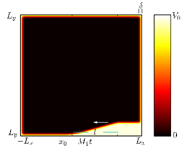
In Section 4.2 we presented the numerical solution of supersonic NLS flow past a corner. The technique used was the same as that presented in [40]. We introduce a linear potential with large contrast that acts as a penalization to flow outside the domain. Such volume penalization methods are well-known in classical fluid dynamics (see, e.g., [54]). In the context of BEC and optics, superfluid flow around obstacles or boundaries are realized in practice using electromagnetic waves or a variable refractive index, both modeled as a spatially varying, linear potential. The benefits of this numerical technique include the use of a regular, Cartesian mesh and highly accurate pseudospectral derivative calculations.

The time-dependent NLS / GP equation (1) with a linear potential

$$i\psi_{t}=-\frac{1}{2}(\psi_{xx}+\psi_{yy})+V(x,y,t)\psi+|\psi|^{2}\psi~,$$ (59)

was solved numerically using a pseudospectral, Fourier spatial discretization and a fourth order Runge-Kutta explicit time stepper. These computations were performed on a rectangular mesh of $N_{x}N_{y}$ equispaced grid points within the domain $[-L_{x},L_{x}]\times[-L_{y},L_{y}]$. Our choice of the potential

$$V(x,y,t) =$$

$$\quad~V_{0}\Big[1-H_{\mu}(L_{x}-|x|-\delta)H_{\mu}(L_{y}-|y|-\delta)$$ (60a)

$$\quad\qquad H_{\mu}(y-C(x-M_{1}t))\Big]~,$$ (60b)

$$C(\xi) =-\tan(\theta)\Big[H_{\mu}(x_{1}-\xi)-H_{\mu}(l)\Big]-L_{y}+\delta~,$$ (60c)

$$H_{\mu}(\xi) =\frac{1}{2}+\frac{1}{2}\tanh(\xi/\mu)~,$$ (60d)

models the boundary conditions corresponding to flow over a corner and also serves to “localize” the solution so that a pseudospectral, Fourier discretization with periodic boundary conditions can be employed. An example potential is shown in Fig. 15. The time-dependent potential corresponds to a moving ramp. The function $H_{\mu}$ is a regularized Heaviside step function with transition width $\mu$. The terms on line (60a) effect the localization of $\psi$ to within $\delta$ of the domain boundaries. The terms on lines (60b) and (60c) correspond to a moving ramp with corner angle $\theta$ and apex located at $(x_{0}-M_{1}t,-L_{y}+\delta)$. When the second corner at $x=x_{0}-M_{1}t+l$ is reached, the ramp flattens and continues as a straight line. The initial condition is the nonlinear, stationary ground state of eq. (59) with potential $V(x,y,0)$ computed by the spectral renormalization technique [55] with the unit density constraint $|\psi(0,0,0)|^{2}=1$. The potential contrast $V_{0}$ is taken sufficiently large so that the density is effectively zero where $V(x,y,t)\approx V_{0}$. Time integration was carried out until the corner reached the left boundary. Near the corner, the flow approximates a “pure” oblique DSW as shown in Fig. 14. Parameter values for table 1 are $N_{x}=4000$, $N_{y}=1000$, $L_{x}=2000$, $L_{y}=500$, $V_{0}=20$, $\delta=2$, $x_{0}=1000$, $l=1000$, $\mu=2$, and a time step of 0.05. The simulation depicted in Fig. 14 results from $N_{x}=3200$, $N_{y}=1600$, $L_{x}=800$, $L_{y}=400$, $V_{0}=20$, $\delta=2$, $x_{0}=400$, $l=400$, $\mu=2$, and a time step of 0.01.

Fig. 15: An example potential $V(x,y,t)$ with $V_{0}\gg 1$ used to model numerical simulation of supersonic flow past a corner. Regions where $V(x,y,t)$ is large correspond to negligible density. The ramp moves to the left with speed $M_{1}$ leading to oblique DSW formation.

6 Discussion and conclusions

One of the motivating questions for this study was the nature of convective versus absolute instabilities of dark solitons. In general, the characterization of the instability type requires knowledge of the dispersion relation for a range of wavenumbers in the complex plane. Unfortunately, the exact discrete spectrum (and hence dispersion relation) for NLS dark solitons is unknown. The formal analysis presented in [11] led to greatly simplified criteria for determining the instability type, which involve only the imaginary (stable) portion of the spectrum.

In this study, the underlying assumptions behind the simplified criteria are exposed and justified using a combination of rigorous results (Theorem 1 and Lemma 15), shallow amplitude asymptotics (Prop. 3), and computations of the spectrum. Consequences of the small-amplitude asymptotics and numerical computations are the first order corrections to the maximal growth rate and associated wavenumber (Corollary 4) and dependence of the critical Mach number on the soliton amplitude (Conclusion 9). Applying Conclusion 9 to the soliton trailing edge of oblique DSWs, we conclude that subsonic oblique DSWs are always absolutely unstable, whereas supersonic oblique DSWs can be absolutely or convectively unstable (Corollaries 12 and 13). In addition, the relationship between stationary DSWs (corner BVPs) and nonstationary DSWs (Riemann IVPs) is studied. In both cases, the DSWs are found to have the same downstream flow properties in the shallow and hypersonic regimes (Conclusion 14).

It is worth contrasting these results with oblique shock waves in classical gas dynamics. Supersonic classical shock fronts in gas dynamics are linearly stable when they satisfy the Lax entropy condition [23]. For the boundary value problem of supersonic flow past a sharp corner, the oblique shock is stable if and only if the downstream flow is supersonic [24, 25]. As far as we know, the distinction between absolute and convective instabilities in the subsonic case has not been elucidated. We note that recent experiments in another viscous medium (granular material) exhibit the stable excitation of oblique DSWs with both supersonic and subsonic downstream flow conditions [56].

Several questions and open problems related to this study are mentioned below.

The nonstationary oblique DSW consists of a slowly modulated elliptic function solution to NLS. How to study the stability or instability of this coherent structure is not immediately obvious given its expanding nature and asymptotic representation. The notion of instability we consider here is centered upon the properties of perturbations to the stationary, trailing dark soliton edge. This is a natural criterion because the soliton trailing edge corresponds to the largest oscillation in the DSW, hence nonlinear effects are strongest there. Another motivation for this choice comes from the numerical simulation of supersonic flow over a corner where the instability first appears along the trailing edge soliton. However, to gain a more complete understanding of DSW instabilities, one should develop an analysis of absolute and convective transverse instabilities of elliptic function solutions. This suggests the more general study of convective/absolute instability for systems with continuous bands of unstable modes. We are not aware of any previous work in this direction.

Careful computations of the spectrum suggest that Conjecture 2 is true. However, to the best of our knowledge, it has not been proven rigorously. It may be possible to do this by reducing the problem to an ODE, where Sturm-Liouville theory is applicable (cf. [57, 30]).

It would be interesting to extend these results to systems with negative dispersion such as shallow water waves where the KP-II equation is valid in the small amplitude regime. In contrast to KP-I studied here, line solitons are linearly stable [28]. Are oblique DSWs in systems with negative dispersion stable?

Acknowledgments. The authors thank Mark Ablowitz for inspiring remarks. The authors also thank Anatoly Kamchatnov for constructive discussions and sharing his recent manuscript [50].

Appendix A Eigenvalue asymptotics

We seek the dispersion relation $\Omega(k;\nu)$ of Eq. (10) for unstable transverse perturbations to the shallow ($0<\nu\ll 1$) dark line soliton (7). Rather than perform asymptotics directly on (10) it is convenient to consider the eigenvalue problem in fluid variables (2). The soliton solution (7) takes the form

$$\rho(x,y,t) =\rho_{s}(\zeta)=1-\nu^{2}\textrm{sech}^{2}(\zeta)~,$$ (61a)

$$u(x,y,t) =u_{s}(\zeta)=\frac{-\kappa}{\sinh^{2}(\zeta)+\frac{\kappa^{2}}{\nu^{2}}\cosh^{2}(\zeta)}~,$$ (61b)

$$v(x,y,t) =0~,\quad\zeta=\nu(x-\kappa t)~.$$ (61c)

Applying multiple scales to (3) leads to the KP-I equation for weakly nonlinear excitations of (1) to the uniform state $\rho~\equiv 1$ (cf. [58]). The scalings involved motivate the following representation of weak transverse perturbations to the dark soliton (61)

$$\rho(x,y,t) =\rho_{s}(\zeta)-\varepsilon f(\zeta)e^{i(p\eta-\Lambda\tau)}~,$$

$$u(x,y,t) =u_{s}(\zeta)-\varepsilon g(\zeta)e^{i(p\eta-\Lambda\tau)}~,$$

$$v(x,y,t) =\varepsilon\nu h(\zeta)e^{i(p\eta-\Lambda\tau)}~,$$

$$\zeta =\nu(x-\kappa t)~,\quad\eta=\nu^{2}y~,\quad\tau=\nu^{3}t~,\quad 0<\varepsilon\ll 1~.$$

Inserting these expansions into (3) and (40c) while keeping only $\mathcal{O}(\varepsilon)$ terms gives

$$-fu_{s}^{\prime}-g\rho_{s}^{\prime}+f^{\prime}\left[\kappa-u_{s}\right]+\rho_{s}\left(-g^{\prime}+ip\nu^{2}h\right) =-i\nu^{2}\Lambda f,$$ (62a)

$$-\frac{\nu^{2}\rho_{s}^{\prime}}{\rho_{s}^{3}}\left(3f^{\prime}\rho_{s}^{\prime}+4f\rho_{s}^{\prime\prime}\right)+\frac{3\nu^{2}f\rho_{s}^{\prime 3}}{\rho_{s}^{4}}+4gu_{s}^{\prime}$$

$$+\frac{\nu^{2}}{\rho_{s}^{2}}\left[\rho_{s}^{\prime}\left(2f^{\prime\prime}-p^{2}\nu^{2}f\right)+2f^{\prime}\rho_{s}^{\prime\prime}(\zeta)+f\rho_{s}^{\prime\prime\prime}\right]$$

$$+4\left[f^{\prime}+g^{\prime}\left(u_{s}-\kappa\right)\right]+\frac{1}{\rho_{s}}\left(p^{2}\nu^{4}f^{\prime}-\nu^{2}f^{\prime\prime\prime}\right) =4i\nu^{2}\Lambda g~,$$ (62b)

$$h^{\prime} =-ipg.$$ (62c)

This is an eigenvalue problem parametrized by $p$ and $\nu$ for the eigenvalue $\Lambda=\Lambda(p;\nu)$ and eigenfunction $[f,g,h]^{T}$.

Assuming $p\notin\{0,\pm p_{\rm cutoff}\}$ where $p_{\rm cutoff}=k_{\rm cutoff}/\nu^{2}$ so that the eigenvalue of interest is simple, we expand the coefficient functions $\rho_{s}$ and $u_{s}$, the parameter $\kappa=\sqrt{1-\nu^{2}}$, the eigenfunction $[f,g,h]^{T}$ and the eigenvalue $\Lambda$ in powers of $\nu^{2}$:

$$f =f_{0}+\nu^{2}f_{1}+\nu^{4}f_{2}+\cdots~,$$

$$g =f_{0}+\nu^{2}g_{1}+\nu^{4}g_{2}+\cdots~,$$ (63)

$$h =-ip\int\left(f_{0}+\nu^{2}g_{1}+\nu^{4}g_{2}+\cdots\right)d\zeta~,$$

$$\Lambda(p;\nu) =\Lambda_{0}(p)+\nu^{2}\Lambda_{1}(p)+\cdots~.$$

Then, (62c) is automatically satisfied to all orders so we only consider eqs. (62a) and (62b) which expand, respectively as

$$\Bigg\{f_{1}^{\prime}-g_{1}^{\prime}+\left[\left(2\text{sech}^{2}(\zeta)-\frac{1}{2}\right)f_{0}\right]^{\prime}+i\Lambda_{0}f_{0}+p^{2}\int f_{0}d\zeta \Bigg\}$$ (64a)

$$+\nu^{2}\Bigg\{f_{2}^{\prime}-g_{2}^{\prime}-\frac{1}{2}\text{sech}^{2}(\zeta)\left(-2\left(f_{1}^{\prime}+g_{1}^{\prime}\right)+f_{0}^{\prime}+2p^{2}\int f_{0}d\zeta\right)$$

$$-\frac{1}{8}f_{0}^{\prime}-\frac{1}{2}f_{1}^{\prime}\text{sech}^{4}(\zeta)f_{0}^{\prime}+\tanh(\zeta)\text{sech}^{2}(\zeta)\left(f_{0}-2\left(f_{1}+g_{1}\right)\right)$$

$$+i\Lambda_{1}f_{0}+i\Lambda_{0}f_{1}-4f_{0}\tanh(\zeta)\text{sech}^{4}(\zeta)+p^{2}\int g_{1}d\zeta \Bigg\}={\cal O}(\nu^{4})~,$$

$$\Bigg\{g_{1}^{\prime}-f_{1}^{\prime}+\left[\left(\text{sech}^{2}(\zeta)-\frac{1}{2}\right)f_{0}\right]^{\prime}+\frac{1}{4}f_{0}^{\prime\prime\prime}+i\Lambda_{0}f_{0} \Bigg\}$$ (64b)

$$+\frac{\nu^{2}}{8}\Bigg\{8g_{2}^{\prime}-8f_{2}^{\prime}+8f_{0}\text{sech}^{2}(\zeta)\tanh(\zeta)\left(2\text{sech}^{2}(\zeta)-1\right)$$

$$+2\text{sech}^{2}(\zeta)\left[-4\tanh(\zeta)\left(f_{0}^{\prime\prime}+2g_{1}\right)+f_{0}^{\prime\prime\prime}+4g_{1}^{\prime}\right]$$

$$+2\text{sech}^{2}(\zeta)\left(6-8\text{sech}^{2}(\zeta)\right)f_{0}^{\prime}-\left(2p^{2}+1\right)f_{0}^{\prime}$$

$$+2f_{1}^{\prime\prime\prime}-4g_{1}^{\prime}+8i\Lambda_{1}f_{0}+8i\Lambda_{0}g_{1} \Bigg\}={\cal O}(\nu^{4})~.$$

A.1 KP eigenvalue problem

Adding (64a) to (64b) gives

$$\frac{1}{4}\left[f_{0}^{\prime\prime\prime}-4\left[(1-3\text{sech}^{2}(\zeta))f_{0}\right]^{\prime}+8i\Lambda_{0}f_{0}+4p^{2}\int f_{0}d\zeta\right]={\cal O}(\nu^{2})~.$$

Differentiating and keeping only leading order terms gives

$$\mathcal{L}f_{0} \doteq f_{0}^{\prime\prime\prime\prime}-4[(1-3\textrm{sech}^{2}\zeta)f_{0}]^{\prime\prime}+8i\Lambda_{0}f_{0}^{\prime}+4p^{2}f_{0}=0~.$$

This is the KP eigenvalue problem studied in [28]. The unstable portion of the spectrum includes one eigenpair

$$f_{0}(\zeta;p) =\frac{d^{2}}{d\zeta^{2}}\left\{e^{\left(1+\sqrt{1-2p/\sqrt{3}}\right)\zeta}\left[2-2p/\sqrt{3}+2\sqrt{1-2p/\sqrt{3}}\right]\left[1-\tanh(\zeta)\right]\right\}~,$$

$$\Lambda_{0}(p) =-i\frac{p}{3}\sqrt{3-2\sqrt{3}p}~,\quad 0<p<\frac{\sqrt{3}}{2}\sim p_{\rm cutoff}~,\quad 0<\nu\ll 1~.$$

This eigenvalue is continued onto the positive real line by the eigenpair

$$f_{0}(\zeta;p) =\frac{d^{2}}{d\zeta^{2}}\left\{e^{\left(1-i\sqrt{2p/\sqrt{3}-1}\right)\zeta}\left[2-2p/\sqrt{3}+2i\sqrt{2p/\sqrt{3}-1}\right]\left[1-\tanh(\zeta)\right]\right\}~,$$

$$\Lambda_{0}(p) =\frac{p}{3}\sqrt{2\sqrt{3}p-3}~,\quad p>\frac{\sqrt{3}}{2}\sim p_{\rm cutoff}~,\quad 0<\nu\ll 1~.$$

A.2 Perturbed KP eigenvalue problem

Below we determine the correction $\Lambda_{1}(p)$. $f_{1}$ is determined in terms of $g_{1}$ by subtracting (64a) from (64b) to obtain

$$2f_{1}^{\prime}-2g_{1}^{\prime}-\frac{1}{4}f_{0}^{\prime\prime\prime}+\left[\text{sech}^{2}(\zeta)f_{0}\right]^{\prime}+p^{2}\int f_{0}d\zeta=\mathcal{O}(\nu^{2})~,$$

so that

$$f_{1} =g_{1}+\frac{1}{8}f_{0}^{\prime\prime}-\frac{1}{2}\text{sech}^{2}(\zeta)f_{0}-\frac{p^{2}}{2}\int\int f_{0}d\zeta+\mathcal{O}(\nu^{2})$$ (65)

$$\doteq g_{1}+\tilde{f}+\mathcal{O}(\nu^{2})~,\quad\tilde{f}=\frac{1}{8}f_{0}^{\prime\prime}-\frac{1}{2}\text{sech}^{2}(\zeta)f_{0}-\frac{p^{2}}{2}\int\int f_{0}d\zeta~.$$

Using (65) in eqs. (64a) and (64b), adding the two equations together and differentiating, the $\mathcal{O}(\nu^{2})$ terms equate to

$$\mathcal{L}g_{1}= ~-\text{sech}^{2}(\zeta)\left[4\left(3f_{0}^{\prime\prime}-p^{2}f_{0}+\tilde{f}^{\prime\prime}+4\tilde{f}\right)+f_{0}^{\prime\prime\prime\prime}\right]$$

$$~+2\tanh(\zeta)\text{sech}^{2}(\zeta)\left(4f_{0}^{\prime}+3f_{0}^{\prime\prime\prime}-4p^{2}\int f_{0}d\zeta+8\tilde{f}^{\prime}\right)$$

$$~+8\text{sech}^{4}(\zeta)\left(2f_{0}^{\prime\prime}-4f_{0}+3\tilde{f}\right)+p^{2}f_{0}^{\prime\prime}-4i\Lambda_{0}\tilde{f}^{\prime}$$

$$~-8\tanh(\zeta)\text{sech}^{4}(\zeta)f_{0}^{\prime}+f_{0}^{\prime\prime}(\zeta)-\tilde{f}^{\prime\prime\prime\prime}+40f_{0}\text{sech}^{6}(\zeta)$$

$$~+2\tilde{f}^{\prime\prime}-8i\Lambda_{1}f_{0}^{\prime}$$

$$~\doteq ~G(\zeta;p)-8i\Lambda_{1}f_{0}^{\prime}~.$$

Solvability then determines $\Lambda_{1}$

$$\Lambda_{1}(p)=-i\frac{\int_{-\infty}^{\infty}G(\zeta;p)h^{*}(\zeta;p)d\zeta}{8\int_{-\infty}^{\infty}f_{0}^{\prime}(\zeta;p)h^{*}(\zeta;p)d\zeta}~,$$ (66)

where $h(\zeta;p)$ is the homogeneous solution of the adjoint problem

$$\mathcal{L}^{\dagger}h=h^{\prime\prime\prime\prime}-4(1-3\textrm{sech}^{2}\zeta)h^{\prime\prime}+8i\Lambda_{0}^{*}h^{\prime}+4p^{2}h=0~.$$

Since $\Lambda_{0}$ is either purely real or purely imaginary, the solution of the adjoint problem is

$$h(\zeta;p)=\left\{\begin{array}[]{cc}f_{0}^{*}(\zeta;p)~,\quad p<\frac{\sqrt{3}}{2}~,\\ f_{0}(\zeta;p)~,\quad p>\frac{\sqrt{3}}{2}\end{array}\right.~.$$

The integrals in (66) can be calculated explicitly

$$\Lambda_{1}(p)=\frac{p^{2}\left(\sqrt{3}-p\right)}{6\sqrt{2\sqrt{3}p-3}}~.$$

For the asymptotic expansion in (63) to be valid, we require $\Lambda_{0}(p)\gg\nu^{2}\Lambda_{1}(p)$. This puts a restriction on the values of $p$ where the expansion is valid:

$$p_{\rm cutoff}<p\ll\frac{1}{\nu^{2}}\quad\mathrm{or}\quad 0<p<p_{\rm cutoff}~,\quad 0<\nu\ll 1~.$$

Then, the unscaled eigenvalue $\Omega(k;\nu)$ in (10) has the asymptotic expansion

$$\Omega(k;\nu) \sim\nu^{3}\Lambda_{0}(k/\nu^{2})+\nu^{5}\Lambda_{1}(k/\nu^{2})~,$$

$$k <k_{\rm cutoff}(\nu)~,\quad k_{\rm cutoff}(\nu)<k=\mathcal{O}(\nu^{2})\ll 1~,\quad 0<\nu\ll 1\,~,$$

which is given in (16).

Appendix B Theorem 1

In [30] it was proved that $L_{0}$ has exactly one negative eigenvalue which was determined explicitly in [8] $(L_{0}+k_{\rm cutoff}^{2}/2)\mathbf{f}=0$. In addition, it was proved in [57] from general considerations of linear operators of the form $JL$ where $J$ is skew-symmetric and $L$ is symmetric, that the number of eigenvalues of $JL$ with a positive real part is at most the number of negative eigenvalues of $L$. The latter decomposition applies to (11), where $L=L_{0}+k^{2}/2$ is symmetric for $k\in\mathbb{R}$ and $J$ is skew-symmetric.

Combining these results, for $0<|k|<k_{\rm cutoff}$, $k\in\mathbb{R}$, $L$ has one negative eigenvalue and therefore $JL$ has at most one eigenvalue with a positive real part. By the instability of the dark soliton, proven in [30], $JL$ has exactly one eigenvalue with positive real part. There is also exactly one eigenvalue with negative real part via the following

Lemma B16.

For $k\in\mathbb{R}$, the eigenvalues of $JL$ come in pairs of opposite sign.

Proof.

For any $k\in\mathbb{R}$,

$$JL\ =\ -R\sigma_{3}LJR\sigma_{3}~.$$ (67)

Let $JL\mathbf{f}=\Gamma\mathbf{f}$. Using (67) and one of the Pauli matrices (53) gives

$$JLR\sigma_{3}\mathbf{f}=-\Gamma R\sigma_{3}\mathbf{f}~.$$

It follows that $(-\Gamma,R\sigma_{3}\mathbf{f})$ is also an eigenpair for $JL$. ∎

On the other hand, for $|k|>k_{\rm cutoff}$, $k\in\mathbb{R}$, $L$ has no negative eigenvalues and therefore, by Lemma B16, $JL$ has only purely imaginary eigenvalues. We find numerically and asymptotically in the shallow regime only two discrete, simple eigenvalues for $k\in\mathbb{C}\setminus\{0,\pm k_{\rm cutoff}\}$.

Appendix C Proof of Lemma 15

We make use of the following identity

$$JL_{0} =\ R\sigma_{1}L_{0}JR\sigma_{1}~.$$ (68)

For any $k\in\mathbb{C}$, consider $(\Omega_{0},\mathbf{f}_{0})$ an eigenpair for eq. (10) satisfying

$$\left[J\left(L_{0}+\frac{1}{2}k^{2}\right)+i\Omega_{0}\right]\mathbf{f}_{0}=0~.$$ (69)

Since $\Omega_{0}$ is a simple eigenvalue, it follows that

$$\dim\left({\rm ker}\left\{\left[JL_{0}+\frac{1}{2}k^{2}J+i\Omega_{0}\right]^{\dagger}\right\}\right)=1~.$$

Therefore, it remains to verify that $R\sigma_{1}\mathbf{f}_{0}^{*}$ is in the nullspace of $[JL_{0}+\frac{1}{2}k^{2}J+i\Omega_{0}]^{\dagger}$. We take the complex conjugate of eq. (69) and apply the decomposition (68) to obtain

$$\left[-R\sigma_{1}L_{0}JR\sigma_{1}+\frac{1}{2}k^{*^{2}}J-i\Omega_{0}^{*}\right]\mathbf{f}_{0}^{*}=0~.$$

Applying $R\sigma_{1}$ yields

$$-\left[L_{0}J+\frac{1}{2}k^{*^{2}}J+i\Omega_{0}^{*}\right]R\sigma_{1}\mathbf{f}_{0}^{*}=0~,$$

which is precisely the adjoint equation to (69). Therefore, we have

$$\ker\left\{\left[J\left(L_{0}+\frac{1}{2}k^{2}\right)+i\Omega_{0}\right]^{\dagger}\right\}=\mathrm{span}\{R\sigma_{1}\mathbf{f}_{0}^{*}\},\quad k\in\mathbb{C}.$$

By similar arguments with $JL_{0}=-\sigma_{2}L_{0}J\sigma_{2}$, one can show that $\sigma_{2}\mathbf{f}_{0}\propto R\sigma_{1}\mathbf{f}_{0}^{*}$ and hence spans the kernel of $[JL_{0}+\frac{1}{2}k^{2}J+i\Omega_{0}]^{\dagger}$ when $k,~\Omega_{0}\in\mathbb{R}$. We use this null eigenfunction in our numerical computations whenever $k\in(k_{\rm cutoff},\infty)$.

References

- [1] Y. S. Kivshar, D. E. Pelinovsky, Self-focusing and transverse instabilities of solitary waves, Phys. Rep. 331 (4) (2000) 117–195.
- [2] D. J. Frantzeskakis, Dark solitons in atomic Bose-Einstein condensates: from theory to experiments, J. Phys. A 43 (21) (2010) 213001.
- [3] T. J. Bridges, Transverse instability of solitary-wave states of the water-wave problem, J. Fluid Mech. 439 (2001) 255–278.
- [4] B. Akers, P. A. Milewski, Dynamics of three-dimensional gravity-capillary solitary waves in deep water, SIAM J. Appl. Math. 70 (7) (2010) 2390–2408.
- [5] B. B. Kadomtsev, V. I. Petviashvili, On the stability of solitary waves in weakly dispersing media, Sov. Phys. Dokl. 15 (1970) 539–541.
- [6] V. E. Zakharov, Instability and nonlinear oscillations of solitons, JETP Lett. 22 (1975) 172–173.
- [7] V. E. Zakharov, A. M. Rubenchik, Instability of waveguides and solitons in nonlinear media, Sov. Phys. JETP 38 (1974) 494–500.
- [8] E. A. Kuznetsov, K. Turitsyn, Instability and collapse of solitons in media with a defocusing nonlinearity, Sov. Phys. JETP 67 (1981) 1583–1586.
- [9] G. A. El, A. Gammal, A. M. Kamchatnov, Oblique dark solitons in supersonic flow of a Bose-Einstein condensate, Phys. Rev. Lett. 97 (18) (2006) 180405.
- [10] Yu. G. Gladush, A. M. Kamchatnov, Z. Shi, P. G. Kevrekidis, D. J. Frantzeskakis, B. A. Malomed, Wave patterns generated by a supersonic moving body in a binary Bose-Einstein condensate, Phys. Rev. A 79 (2009) 033623.
- [11] A. M. Kamchatnov, L. P. Pitaevskiĭ, Stabilization of solitons generated by a supersonic flow of Bose-Einstein condensate past an obstacle, Phys. Rev. Lett. 100 (2008) 160402.
- [12] P. A. Sturrock, Kinematics of growing waves, Phys. Rev. 112 (5) (1958) 1488–1503.
- [13] R. G. Briggs, Electron-Stream Interaction with Plasmas, MIT Press, Cambridge, Mass., 1964.
- [14] C. M. Dafermos, Hyperbolic Conservation Laws in Continuum Physics, 3rd Edition, Springer, 2009.
- [15] M. A. Hoefer, M. J. Ablowitz, Dispersive shock waves, Scholarpedia 4 (11) (2009) 5562.
- [16] Z. Dutton, M. Budde, C. Slowe, L. V. Hau, Observation of quantum shock waves created with ultra-compressed slow light pulses in a Bose-Einstein condensate, Science 293 (2001) 663.
- [17] M. A. Hoefer, M. J. Ablowitz, I. Coddington, E. A. Cornell, P. Engels, V. Schweikhard, Dispersive and classical shock waves in Bose-Einstein condensates and gas dynamics, Phys. Rev. A 74 (2006) 023623.
- [18] R. Meppelink, S. B. Koller, J. M. Vogels, P. van der Straten, E. D. van Ooijen, N. R. Heckenberg, H. Rubinsztein-Dunlop, S. A. Haine, M. J. Davis, Observation of shock waves in a large Bose-Einstein condensate, Phys. Rev. A 80 (4) (2009) 043606.
- [19] W. Wan, S. Jia, J. W. Fleischer, Dispersive superfluid-like shock waves in nonlinear optics, Nat. Phys. 3 (1) (2007) 46–51.
- [20] C. Conti, A. Fratalocchi, M. Peccianti, G. Ruocco, S. Trillo, Observation of a gradient catastrophe generating solitons, Phys. Rev. Lett. 102 (8) (2009) 083902.
- [21] A. Armaroli, S. Trillo, A. Fratalocchi, Suppression of transverse instabilities of dark solitons and their dispersive shock waves, Phys. Rev. A 80 (5).
- [22] M. A. Hoefer, B. Ilan, Theory of two-dimensional oblique dispersive shock waves in supersonic flow of a superfluid, PRA 80 (2009) 061601(R).
- [23] A. Majda, The stability of multidimensional shock fronts, Mem. Amer. Math. Soc. 275.
- [24] D. Li, Analysis on linear stability of oblique shock waves in steady supersonic flow, J. Diff. Eq. 207 (1) (2004) 195–225.
- [25] D. L. Tkachev, A. M. Blokhin, Courant-Friedrich’s hypothesis and stability of the weak shock, Proc. Symp. Appl. Math. 67 (2) (2009) 959.
- [26] K. Zumbrun, H. K. Jenssen, G. Lyng, Stability of large-amplitude shock waves of compressible Navier-Stokes equations, in: S. Friedlander, D. Serre (Eds.), Handbook of Mathematical Fluid Dynamics, Vol. 3, Elsevier, Amsterdam, 2005, pp. 311–533.
- [27] R. Courant, K. O. Friedrichs, Supersonic Flow and Shock Waves, Springer-Verlag, Berlin, 1948.
- [28] J. C. Alexander, R. L. Pego, R. L. Sachs, On the transverse instability of solitary waves in the Kadomtsev-Petviashvili equation, Phys. Lett. A 226 (3-4) (1997) 187–192.
- [29] D. Pelinovsky, Y. Stepanyants, Y. Kivshar, Self-focusing of plane dark solitons in nonlinear defocusing media, Phys. Rev. E 51 (5) (1995) 5016–5026.
- [30] F. Rousset, N. Tzvetkov, A simple criterion of transverse linear instability for solitary waves, Math. Res. Lett. 17 (1) (2010) 157–169.
- [31] L. P. Pitaevskiĭ, E. Lifshitz, Physical Kinetics, Vol. 10 of Course of Theoretical Physics, Pergamon Press, Oxford, England, 1981, Ch. 62, pp. 268–273.
- [32] E. Infeld, G. Rowlands, Nonlinear Waves, Solitons and Chaos, Cambridge University Press, Cambridge, UK, 1990.
- [33] P. J. Schmid, D. S. Henningson, Stability and Transition in Shear Flows, Vol. 142 of Applied Mathematical Sciences, Springer-Verlag, New York, 2000.
- [34] A. Bers, Space-time evolution of plasma instabilities–absolute and convective, Vol. 1, Elsevier, Amsterdam: North-Holland, 1983, pp. 451–517.
- [35] P. Huerre, P. A. Monkewitz, Absolute and convective instabilities in free shear layers, Journal of Fluid Mechanics 159 (1985) 151–168.
- [36] L. Brevdo, T. J. Bridges, Absolute and convective instabilities of spatially periodic flows, Phil. Trans. R. Soc. Lond. A 354 (1710) (1996) 1027–1064.
- [37] P. D. Miller, Applied Asymptotic Analysis, AMS Publications, Providence, 2006.
- [38] V. A. Mironov, A. I. Smirnov, L. A. Smirnov, Structure of vortex shedding past potential barriers moving in a Bose-Einstein condensate, JETP 110 (5) (2010) 877–889.
- [39] G. A. El, A. M. Kamchatnov, V. V. Khodorovskii, E. S. Annibale, A. Gammal, Two-dimensional supersonic nonlinear Schrödinger equation flow past an extended obstacle, Phys. Rev. E 80 (2009) 046317.
- [40] M. A. Hoefer, B. Ilan, Theory of two-dimensional oblique dispersive shock waves in supersonic flow of a superfluid, Phys. Rev. A 80 (6) (2009) 061601(R).
- [41] G. B. Whitham, Non-linear dispersive waves, Proc. Roy. Soc. Ser. A 283 (1965) 238–261.
- [42] A. V. Gurevich, L. P. Pitaevskiĭ, Nonstationary structure of a collisionless shock wave, Sov. Phys. JETP 38 (2) (1974) 291–297.
- [43] A. V. Gurevich, A. L. Krylov, Dissipationless shock waves in media with positive dispersion, Sov. Phys. JETP 65 (5) (1987) 944–953.
- [44] G. A. El, R. H. J. Grimshaw, N. F. Smyth, Unsteady undular bores in fully nonlinear shallow-water theory, Phys. Fluids 18 (2) (2006) 027104.
- [45] G. A. El, A. Gammal, E. G. Khamis, R. A. Kraenkel, A. M. Kamchatnov, Theory of optical dispersive shock waves in photorefractive media, Phys. Rev. A 76 (5) (2007) 053813.
- [46] G. A. El, Resolution of a shock in hyperbolic systems modified by weak dispersion, Chaos 15 (2005) 037103.
- [47] A. V. Gurevich, A. L. Krylov, V. V. Khodorovskii, G. A. El, Supersonic flow past bodies in dispersive hydrodynamics, Sov. Phys. JETP 81 (1995) 87–96.
- [48] A. V. Gurevich, A. L. Krylov, V. V. Khodorovskii, G. A. El, Supersonic flow past finite-length bodies in dispersive hydrodynamics, Sov. Phys. JETP 82 (1996) 709–718.
- [49] G. A. El, A. M. Kamchatnov, Spatial dispersive shock waves generated in supersonic flow of Bose-Einstein condensate past slender body, Phys. Rev. A 350 (3-4) (2006) 192–196.
- [50] A. M. Kamchatnov, S. V. Korneev, Condition for convective instability of dark solitons, arXiv:1105.0789 [cond-mat.quant-gas].
- [51] W. D. Hayes, R. F. Probstein, Hypersonic Inviscid Flow, Dover, 2004.
- [52] M. A. Hoefer, M. J. Ablowitz, P. Engels, Piston dispersive shock wave problem, Phys. Rev. Lett. 100 (2008) 084504.
- [53] A. Kamchatnov, S. Korneev, Flow of a Bose-Einstein condensate in a quasi-one-dimensional channel under the action of a piston, JETP 110 (1) (2010) 170–182.
- [54] G. Keetels, U. D’Ortona, W. Kramer, H. Clercx, K. Schneider, G. van Heijst, Fourier spectral and wavelet solvers for the incompressible Navier-Stokes equations with volume-penalization: Convergence of a dipole-wall collision, J. Comp. Phys. 227 (2) (2007) 919–945.
- [55] M. J. Ablowitz, Z. H. Musslimani, Spectral renormalization method for computing self-localized solutions to nonlinear systems, Opt. Lett. 30 (2005) 2140–2142.
- [56] J. M. N. T. Gray, X. Cui, Weak, strong and detached oblique shocks in Gravity-Driven granular Free-Surface flows, J. Fluid Mech. 579 (2007) 113–136.
- [57] R. L. Pego, M. I. Weinstein, Eigenvalues, and instabilities of solitary waves, Phil. Trans. Roy. Soc. London Ser. A 340 (1656) (1992) 47–94.
- [58] V. Zakharov, E. Kuznetsov, Multi-scale expansions in the theory of systems integrable by the inverse scattering transform, Physica D 18 (1-3) (1986) 455–463.