A study of variable selection using $g$-prior distribution with ridge parameter

Abstract

In the Bayesian variable selection framework, a common prior distribution for the regression coefficients is the $g$-prior of Zellner [1986]. However, there are two standard cases in which the associated covariance matrix does not exist, and the conventional prior of Zellner can not be used: if the number of observations is lower than the number of variables (large $p$ and small $n$ paradigm), or if some variables are linear combinations of others. In such situations a prior distribution derived from the prior of Zellner can be used, by introducing a ridge parameter. The prior obtained is a flexible and simple adaptation of the $g$-prior, and can be linked to the work of Gupta and Ibrahim [2007]. In this paper a simple way to choose the associated hyper-parameters is proposed. The method is valid for any generalized linear mixed model and we focus on the case of variable selection for probit mixed models when some variables are linear combinations of others. The method is then applied to both simulated and real datasets obtained from Affymetrix microarray experiments.

1 Introduction

We consider the problem of bayesian variable selection in a generalized linear mixed model with $Y$ a $n$-vector of responses, given a set of $p$ potential fixed regressors

$$g(\mathbb{E}(Y_{i}\mid U,\beta))=X_{i}^{T}\beta+Z_{i}^{T}U,$$

where $g$ stands for the link function associated to the model, and $X_{i}$ and $Z_{i}$ for the fixed and random effect regressors associated to the $i$th observation. The parameter $\beta\in\mathbb{R}^{p}$ corresponds to the fixed-effect coefficients and the parameter $U$ to the random-effect coefficients. $X$ and $Z$ are known design matrices associated with the fixed and random effects. We consider $K$ random effects, $U=(U_{1}^{T},\cdots,U_{K}^{T})^{T}$ where each $U_{l}$ is a vector of size $q_{l}$, and $\sum_{l=1}^{K}q_{l}=q$.

When the purpose is to select relevant variables among the $p$ candidates, it is convenient to denote by $\gamma$ the vector of latent variables indicating if a variable is selected or not; that is, $\gamma_{j}=1$ if $\beta_{j}\neq 0$ and $\gamma_{j}=0$ if $\beta_{j}=0$. We then denote by $\beta_{\gamma}$ the vector of all nonzero elements of $\beta$ and by $\mathbf{X}_{\gamma}$ the design matrix with columns corresponding to the elements of $\gamma$ that are equal to 1.

To complete the model, a conventional prior distribution for $\beta_{\gamma}|\gamma$ is a $d_{\gamma}$-dimensional Gaussian distribution, with $d_{\gamma}=\sum_{j=1}^{p}\gamma_{j}$,

$$\beta_{\gamma}|\gamma\sim{\cal N}_{d_{\gamma}}(0,\Sigma_{\gamma}).$$ (1)

Concerning the prior covariance matrix $\Sigma_{\gamma}$, an attractive and standard choice is

$$\Sigma_{\gamma}=\tau(\mathbf{X}_{\gamma}^{\prime}\mathbf{X}_{\gamma})^{-1}.$$ (2)

Equations (1) and (2) correspond to the g-prior distribution, proposed by Zellner [1986] in the case of standard linear models. This prior replicates the covariance structure of the design and enables an automatic scaling based on the data. Up to the scalar $\tau$, the prior covariance matrix is related to the Fisher Information Matrix in the linear model (see for instance Chen and Ibrahim [2003]). Moreover, it leads to simple expressions of the marginal likelihood, and as pointed out in George and Foster [2000], the marginal likelihood becomes a function of both R-square and the number of covariates like in AIC or BIC criteria. The parameter $\tau>0$ is referred to as the variable selection coefficient in Bottolo and Richardson [2010]. In the homoscedastic linear model with variance $\sigma^{2}$, this parameter can be expressed as $\tau=g\sigma^{2}$. Therefore this prior has been used by many authors in case of linear models, but also for generalized linear models. In case of a binary response variable, this prior is frequently encountered in probit models which are quite practical in a Bayesian setting (see Lee et al. [2003], Sha et al. [2004], Zhou et al. [2004] and Yang and Song [2010] for instance).

The choice of the variable selection coefficient $\tau$ can have a great influence on the variable selection process (see George and Foster [2000]) and has been considered by many authors. Some of them considered a fixed value for $\tau$. For instance Smith and Kohn [1997] suggested to choose $\tau$ between 10 and 100. Another approach is the approach of George and Foster [2000], who developed empirical Bayes methods based on the estimation of $\tau$ from its marginal likelihood. Other authors proposed to put a hyper-prior distribution on $\tau$, like Zellner and Siow [1980] that used an inverse-gamma distribution $\mathcal{IG}(1/2,n/2)$. But under the Zellner-Siow prior, marginal likelihoods are not available in closed forms, and approximations are necessary (see Bottolo and Richardson [2010]). Note also that the Zellner-Siow prior can be represented as a mixture of g-priors. Following this remark, Liang et al. [2008] proposed a new family of priors on $\tau$, the hyper-g prior family which leads to new mixtures of $g$-priors while maintaining the computational tractability of the marginal likelihoods. Independently but in the same spirit, Cui and George [2008] suggested to put an inverse-gamma prior distribution on $(1+\tau)$ (rather than on $\tau$ like Zellner and Siow), obtaining a family of priors on $\tau$ which contains the hyper-g prior family as a special case. Marin and Robert [2007] also proposed a way to use mixtures of $g$-prior for model selection.

In spite of the variety of all these works to choose the variable selection coefficient $\tau$, a crucial problem remains with priors using the matrix $(\mathbf{X}_{\gamma}^{T}\mathbf{X}_{\gamma})^{-1}$. Indeed, $\mathbf{X}_{\gamma}^{T}\mathbf{X}_{\gamma}$ should be invertible. However, there are two standard cases where $\mathbf{X}_{\gamma}^{T}\mathbf{X}_{\gamma}$ is singular:

• If the number of observations is lower than the number of variables in the model, $n<d_{\gamma}$.

• If some variables are linear combinations of others. In practice, even if $\mathbf{X}_{\gamma}^{T}\mathbf{X}_{\gamma}$ is theoretically invertible, some variables can be highly correlated and $\mathbf{X}_{\gamma}^{T}\mathbf{X}_{\gamma}$ can be computationally singular. It is often the case in genomic high-dimensional datasets for example. This problem can also be encountered when several datasets are merged: some variables can be collinear or almost collinear if same variables were present into several datasets under different labels for instance.

In these cases the classical $g$-prior does not work. Concerning the first case, several authors proposed alternative priors. In case of linear models, Maruyama and George [2010] proposed a generalization of the $g$-prior. In case of probit models, Yang and Song [2010] proposed to replace the matrix $(\mathbf{X}_{\gamma}^{T}\mathbf{X}_{\gamma})^{-1}$ in $\Sigma_{\gamma}$ by its Moore Penrose’s inverse (see alsoWest [2003]). However, the computation of the posterior distribution proposed by Yang and Song [2010] has a technical issue that do not permit the use of MCMC algorithm (see Baragatti and Pommeret [2011]). Another idea would be to avoid this first case by fixing the number of selected covariates at each iteration, as in Baragatti [2011]. It is a practical way when the purpose is to retain only few regressors, because it appeared computationally advantageous and it reduced the effect of the variable selection coefficient $\tau$ used in the $g$-prior. But the number of selected variables at each iteration must be arbitrarily fixed. Moreover, fixing the number of selected covariates is not a solution for the second case, as well as the priors proposed by Maruyama and George [2010] and Yang and Song [2010]. For linear model, Brown et al. [1998] proposed to work with transformations of $X$ and $Y$, using a Singular Values Decomposition in the spirit of the ridge regression (see Marquardt [1970]). This numerical approach was extended to multivariate general linear models in Brown et al. [2002]. Always in the spirit of ridge regression, Gupta and Ibrahim [2007] proposed an extension of the $g$-prior. They introduced a ridge parameter, and considered generalized linear models. Their prior can be used in the two cases, but they did not study the second case in which some variables are linear combinations of others. More generally, to our knowledge the problem of variable selection in generalized linear mixed models when some variables are linear combinations of others is not present in literature.

In this paper we develop the idea of Gupta and Ibrahim [2007] concerning the introduction of ridge parameter, in a slightly different form. Besides, we suggest a way to choose the associated hyper-parameters: following the original idea of Zellner which is to keep the covariance structure of the design, we propose to keep the total variance of the data through the trace of $\mathbf{X}^{T}\mathbf{X}$. We focused on probit models, as studied in Baragatti (2011), Yang and Song [2010] and Lee et al. [2003]. The aim is to study the behavior of the variable selection process while using the proposed prior, especially when some variables are linear combinations of others. The approach developed is applied both to simulation data, and to data obtained from Affymetrix microarray experiments.

This paper is organized as follows. In Section 2 the extension of the prior to be used for $\beta_{\gamma}$ is introduced and a choice for the hyper-parameters is suggested. The section 3 outlines the priors, full conditional distributions and the sampler to be used in case of a probit mixed model. In Section 4 experimental results are given and a sensitivity analysis is performed. Finally Section 5 discusses the method.

2 Introducing a ridge parameter

2.1 Prior distribution of $\beta$ with a ridge parameter

As previously explained, in case of singularity of the matrix $\mathbf{X}_{\gamma}^{T}\mathbf{X}_{\gamma}$, the classical $g$-prior can not be used. We propose to introduce a ridge parameter, denoted $\lambda>0$, by replacing in (2) the matrix $\tau^{-1}\mathbf{X}_{\gamma}^{T}\mathbf{X}_{\gamma}$ by $\tau^{-1}\mathbf{X}_{\gamma}^{T}\mathbf{X}_{\gamma}+\lambda I$. We get

$$\beta_{\gamma}|\gamma\sim{\cal N}_{d_{\gamma}}\big(0,(\tau^{-1}\mathbf{X}_{\gamma}^{T}\mathbf{X}_{\gamma}+\lambda I)^{-1}\big)\qquad\textrm{with}\qquad d_{\gamma}=\sum_{j=1}^{p}\gamma_{j}.$$ (3)

We write

$$\Sigma_{\gamma}(\lambda)=(\tau^{-1}\mathbf{X}_{\gamma}^{T}\mathbf{X}_{\gamma}+\lambda I)^{-1}.$$ (4)

When $\lambda>0$, the matrix $\Sigma_{\gamma}(\lambda)$ is always of full rank. We obtain a modified form of the $g$-prior, which is a compromise between independence and instability. Indeed, for large values of $\lambda$ and $\tau$, $\Sigma_{\gamma}(\lambda)$ is close to a diagonal matrix that coincides with the conditional independent case. On the opposite, for small values of $\lambda$ and $\tau$, the term $\tau^{-1}\mathbf{X}_{\gamma}^{T}\mathbf{X}_{\gamma}$ prevails and the inverse of $\tau^{-1}\mathbf{X}_{\gamma}^{T}\mathbf{X}_{\gamma}+\lambda I$ will be instable if $\mathbf{X}_{\gamma}^{T}\mathbf{X}_{\gamma}$ is singular. In that case, the prior distribution (3) is close to the $g$-prior case. In comparison, the prior of Gupta and Ibrahim [2007] uses $\Sigma_{\gamma}(\lambda)=\tau(\mathbf{X}_{\gamma}^{T}\mathbf{X}_{\gamma}+\lambda I)^{-1}$ (with an additional parameter $\sigma^{2}$ because they focused on the linear case). Note that the classical $g$-prior corresponds to a special case of (4), with $\lambda=0$.

2.2 Calibrating hyper-parameters

Following Zellner [1986], our purpose is to use the design to calibrate the covariance of $\beta_{\gamma}$ with a ridge parameter. Write $\Sigma_{\gamma}(0)=\tau_{0}(\mathbf{X}_{\gamma}^{T}\mathbf{X}_{\gamma})^{-1}$, with $\tau_{0}$ the fixed hyper-parameter used in this classical prior. Using $\Sigma_{\gamma}(\lambda)$ instead of $\Sigma_{\gamma}(0)$ amounts to introducing a perturbation in the classical $g$-prior. An interesting feature of the classical $g$-prior is that the variance-covariance structure of the data is preserved. The ridge parameter prevents us to strictly preserve this structure. However, it is possible to replicate the total variance of the data, which corresponds, up to a normalization, to the trace of $\Sigma_{\gamma}(0)^{-1}$. The constraint used is then

$$tr\Big(\Sigma_{\gamma}(0)^{-1}\Big)=tr\Big(\Sigma_{\gamma}(\lambda)^{-1}\Big),$$

which yields

$$\tau=\tau_{0}\Big[1+\displaystyle\frac{\lambda p\tau_{0}}{tr(\mathbf{X}_{\gamma}^{T}\mathbf{X}_{\gamma})-\lambda p\tau_{0}}\Big].$$

Concerning the choice of $\lambda$, in order to take into account the number $p$ of covariates and to reduce the effect of the ridge factor, we suggest to take $\lambda=1/p$, getting

$$\tau=\tau_{0}\Big[1+\displaystyle\frac{\tau_{0}}{tr(\mathbf{X}_{\gamma}^{T}\mathbf{X}_{\gamma})-\tau_{0}}\Big].$$

The vector $\gamma$ can be different between two iterations of the algorithm. Therefore we propose to use the complete design matrix $\mathbf{X}$ instead of $\mathbf{X}_{\gamma}$, yielding

$$\tau=\tau_{0}\Big[1+\displaystyle\frac{\tau_{0}}{tr(\mathbf{X}^{T}\mathbf{X})-\tau_{0}}\Big].$$ (5)

In practice, the user has to choose only the parameter $\tau_{0}$, $\lambda$ and $\tau$ are then obtained by $1/p$ and (5). Following Smith and Kohn [1997], $\tau_{0}$ can be chosen between 10 and 100. In section 4.3, the sensitivity analysis will assess the influence of the values of these hyper-parameters $\lambda$ and $\tau$.

2.3 Other prior distributions

The $\gamma_{j}$ are assumed to be independent Bernoulli variables, with

$$P(\gamma_{j}=1)=\pi_{j},\qquad 0\leq\pi_{j}\leq 1\qquad j=1,\ldots,p$$ (6)

If we do not want to use prior knowledge to favor any variables, we put $\pi_{j}=\pi,\forall j\in\{1,\ldots,p\}$.
The vector of coefficients associated with the random effects is assumed to be Gaussian and centered, with covariance matrix $D$:

$$U|D\sim{\cal N}_{q}(0,D).$$ (7)

We will consider the case where $D$ is a diagonal matrix $D=diag(A_{1},\ldots,A_{K})$, where $A_{l}=\sigma_{l}^{2}I_{q_{l}}$, $l=1,\ldots,K$ and $I_{q_{l}}$ the identity matrix. The prior distributions for the $\sigma_{l}^{2}$ are then Inverse Gamma $\mathcal{IG}(a,b)$ ($b$ denoting the scale parameter). In a more general case, if no structure is assumed for the variance-covariance matrix $D$, its prior distribution should be an Inverse-Wishart.

3 Illustration trough a mixed probit model

3.1 The probit mixed model

We consider the problem of variable selection in the model given a set of $p$ potential fixed regressors

$$P(Y_{i}=1\mid U,\beta)=p_{i}=\Phi(X_{i}^{T}\beta+Z_{i}^{T}U),$$

where $\Phi$ stands for the standard Gaussian cumulative distribution function. Following Albert and Chib [1993] and Lee et al. [2003], a vector of latent variables $L=(L_{1},\ldots,L_{n})^{T}$ is introduced, and we assume that the conditional distribution of $L$ is Gaussian, written $L\mid U,\beta\sim\mathcal{N}_{n}(X\beta+ZU,I_{n})$, with $I_{n}$ the identity matrix. We then have

$$Y_{i}=\left\{\begin{array}[]{rl}1&\text{if }L_{i}>0\\ 0&\text{if }L_{i}<0.\end{array}\right.$$ (8)

3.2 Sampler description

The posterior distribution of $\gamma$ is of particular interest for the variable selection problem. An idea is to use a Gibbs sampler to explore this posterior distribution and to search for high probability $\gamma$ values. Simulations from all full conditional distributions can be easily obtained, except for $\gamma$ which full conditional distribution does not correspond to a standard multivariate one. The $\gamma$ vector can be simulated either element by element, or by using a Metropolis-Hastings algorithm. In general, in case of a high number of variables, the Metropolis-Hastings algorithm is computationally advantageous. Moreover, using a Metropolis-Hastings step in a Gibbs sampler improves the sampler in terms of variance, see Robert and Casella [2004]. As a consequence, we decided to use a Metropolis-within-Gibbs algorithm. But even with a Metropolis-Hastings algorithm, the full conditional distribution of $\gamma$ cannot be directly simulated, since it depends on the actual value of $\beta_{\gamma}$. Therefore following Lee et al. [2003] and Baragatti [2011], we used the grouping technique of Liu [1994], by considering the parameters $\gamma$ and $\beta_{\gamma}$ jointly. The advantage of this technique is that the convergence of the Markov chain is improved, and autocorrelations are reduced, see Liu [1994] and van Dyk and Park [2008].

Most of the full conditional distributions did not depend on the ridge parameter, and were the same than those in Baragatti (2011). Only those of $\beta_{\gamma}$ and $\gamma$ depend on $\lambda$, as follows:

$$\beta_{\gamma}|L,U,\gamma\sim\mathcal{N}_{d_{\gamma}}(V_{\gamma}\mathbf{X}_{\gamma}^{T}(L-ZU),V_{\gamma})\quad\textrm{with}\quad V_{\gamma}=\Big[\frac{(1+\tau)}{\tau}\mathbf{X}_{\gamma}^{T}\mathbf{X}_{\gamma}+\lambda I\Big]^{-1},$$ (9)

where $d_{\gamma}=\sum_{j=1}^{p}\gamma_{j}$, and

$$f(\gamma|L,U) \propto \displaystyle\frac{|V_{\gamma}|^{1/2}}{|\Sigma_{\gamma}(\lambda)|^{1/2}}\exp\Big[-\frac{1}{2}((L-ZU)^{T}(I-\mathbf{X}_{\gamma}V_{\gamma}\mathbf{X}_{\gamma}^{T})(L-ZU)\Big]$$ (10)

$$\times \displaystyle\prod_{j=1}^{p}\pi_{j}^{\gamma_{j}}(1-\pi_{j})^{1-\gamma_{j}}.$$

Setting $\lambda=0$, we recognize the formula obtained by Baragatti (2011) in case of a classical $g$-prior.

Remark 1

The influence of $\tau$ appears here through the ratio $R^{1/2}=\left(\frac{|V_{\gamma}|}{|\Sigma_{\gamma}|}\right)^{1/2}$. We can see that

$$\left\{\begin{array}[]{ll}{\rm if\ }\tau\rightarrow\infty,&R\rightarrow|\frac{1}{\lambda}\mathbf{X}_{\gamma}^{T}\mathbf{X}_{\gamma}+I|^{-1},\\ {\rm if\ }\tau\rightarrow 0,&R\rightarrow 1.\end{array}\right.$$

The Metropolis-Hastings algorithm used to generate the $\gamma$ vector can be summarized as follows: at iteration $(i+1)$ a candidate $\gamma^{*}$ is proposed from $\gamma^{(i)}$, and using a symmetric transition kernel the acceptance rate is

$$\rho(\gamma^{(i)},\gamma^{*})=\min\Bigg\{1,\displaystyle\frac{f(\gamma^{*}|L,U)}{f(\gamma^{(i)}|L,U)}\Bigg\},$$

with

$$\displaystyle\frac{f(\gamma^{*}|L,U)}{f(\gamma^{(i)}|L,U)} = \displaystyle\left(\frac{|V_{\gamma^{*}}\Sigma_{\gamma^{(i)}}|}{|\Sigma_{\gamma^{*}}V_{\gamma^{(i)}}|}\right)^{1/2}\exp\Big\{-\frac{1}{2}(L-ZU)^{T}(\mathbf{X}_{\gamma^{i}}V_{\gamma^{(i)}}\mathbf{X}_{\gamma^{(i)}}^{T}-\mathbf{X}_{\gamma^{*}}V_{\gamma^{*}}\mathbf{X}_{\gamma^{*}}^{T})(L-ZU)\Big\}$$ (11)

$$\times \displaystyle\prod_{j=1}^{p}\left(\displaystyle\frac{\pi_{j}}{1-\pi_{j}}\right)^{\gamma_{j}^{*}-\gamma_{j}^{(i)}},\qquad\textrm{if}\qquad\forall j\in\{1,\ldots,p\}\quad\pi_{j}=\pi.$$

The simplest way to have a symmetric transition kernel is to propose a $\gamma^{*}$ which corresponds to $\gamma^{(i)}$ in which $r$ components have been randomly changed (see Chipman et al. [2001] and George and McCulloch [1997]).

Remark 2

The influence of $\tau$ appears via the ratio $Q^{1/2}=\left(\frac{|V_{\gamma^{*}}\Sigma_{\gamma^{(i)}}|}{|\Sigma_{\gamma^{*}}V_{\gamma^{(i)}}|}\right)^{1/2}$ that satisfies:

$$\left\{\begin{array}[]{ll}{\rm if\ }\tau\rightarrow\infty,&Q\rightarrow|\mathbf{X}_{\gamma^{*}}^{T}\mathbf{X}_{\gamma^{*}}+\lambda I|\times|\mathbf{X}_{\gamma^{i}}^{T}\mathbf{X}_{\gamma^{i}}+\lambda I|^{-1},\\ {\rm if\ }\tau\rightarrow 0,&Q\rightarrow 1.\end{array}\right.$$

3.3 Post-processing

The number of iterations of the algorithm is $b+m$, where $b$ corresponds to the burn-in period and $m$ to the observations from the posterior distributions. For selection of variables, the sequence $\{\gamma^{(t)}=(\gamma_{1}^{(t)},\ldots,\gamma_{p}^{(t)}),t=b+1,\ldots,b+m\}$ is used. The most relevant variables for the regression model are those which are supported by the data and prior information. Thus they are those corresponding to the $\gamma$ components with higher posterior probabilities, and can be identified as the $\gamma$ components that are most often equal to 1. To decide which variables should be finally selected after a run, a confidence interval based on a Poisson distribution could be used. However we noticed that usually a reasonable number of relevant variables can be isolated from the other ones concerning the number of selections. Then we suggest to use a box-plot of the number of iterations during which variables were selected. For each run the variables distinguishable from others can be selected by fixing a threshold: if a variable has been selected during a number of iterations which is higher than this threshold, then the variable is kept in the final selection.

4 Experimental results

4.1 Simulated data

We simulated 200 binary observations and 300 variables, the observations being obtained using a probit mixed model with 5 of these variables and one random effect of length 4. Among the 300 variables, 280 were generated from a uniform on $[-5,5]$ and denoted by $V1,\ldots,V280$. Then 10 variables denoted by $V281,\ldots,V290$ were build to be collinear to the first 10 variables, with a factor 2: for instance $V282=2\times V2$. One variable was build to be a linear combination of $V1$ and $V2$ ($V291=V1+V2$), and another was build to be a linear combination of $V3$ and $V4$ ($V292=V3-V4$). Finally, 8 variables were build to be linear combinations of variables 5 to 12 and variables 13 to 20 (for instance $V293=V5+V13$). The five variables used to generate the binary observations were the first five: $V1,V2,V3,V4$ and $V5$. The vector of coefficients associated with these variables was $\beta=(1,-1,2,-2,3)$. The first 100 observations were part of the training set, and the last 100 were part of the validation set. In the training and the validation sets, 25 observations were associated with each component of the random effect, whom vector of coefficients was $U=(-3,-2,2,3)$. We had only one random effect and the different components were supposed independent, hence we put $D=\sigma^{2}I_{4}$ with an inverse-gamma prior $\mathcal{IG}(a,b)$ for $\sigma^{2}$.

The objective was to assess the behavior of the proposed method when some variables are linear combinations of others, and to compare it to the case where no variable is linear combination of others. Therefore we performed 10 runs of the algorithm using only the first 280 variables, and 10 runs using the 300 variables. In these two cases and for each run the same parameters were used: 5 variables were initially selected, one component of $\gamma$ was proposed to be changed at each iteration of the Metropolis-Hastings step, the prior of $\sigma^{2}$ was a $\mathcal{IG}(1,1)$, $\pi_{j}=5/280$ for all $j$ when 280 variables were kept, $\pi_{j}=5/300$ for all $j$ when 300 variables were kept, 4000 iterations were performed after a burn-in period of 1000 iterations, and each Metropolis-Hastings step consisted of 500 iterations. We decided to choose $\tau_{0}=50$, which is a standard choice, see Smith and Kohn [1997] for instance. The parameters $\lambda$ and $\tau$ were then chosen as explained in 2.2, yielding $\lambda=1/280$ and $\tau=50.01075$ when using 280 variables, and $\lambda=1/300$ and $\tau=50.00885$ when using 300 variables.

A final selection was performed for each of the 20 runs. Figure 1 presents two boxplots associated to 280 variables and 300 variables, respectively. For the run with 280 variables there is a gap between the variables $V2,V3,V4$ and $V5$ and the others, hence we selected these four variables. For the run with 300 variables: there is a gap between the variables selected in more than 400 iterations and the others, hence we selected the eight corresponding variables.

Figure 1: Boxplots of the number of selections of a variable after the burn-in period. Each point represents a variable (or several variables if superposed). The left boxplot corresponds to the run 5 with 280 variables. The right boxplot corresponds to the run 6 with 300 variables.

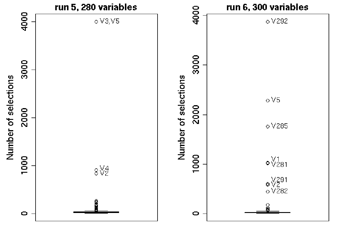
Table 1 gives the variables kept in the final selections of the 20 runs. Among the runs with the first 280 variables, 3 among the 5 variables used to generate the data were in the final selection of almost all runs, and the variables $V4$ was in the final selection of half of the runs. Notice that $V1$ was in none of the final selections. Among the runs with 300 variables, the variables $V1,V2,V3$ and $V5$ were present in most of the final selections, directly or indirectly through linear combinations. Contrarily to the runs with 280 variables, the variables $V4$ or $V284$ were in none of the final selections, while the variables $V1$ and $V281$ were in all the final selections. Concerning $V4$, it was indirectly in all the final selections through $V292$, which is a linear combination of $V3$ and $V4$. Eventually, the final selections of the runs with 300 variables appeared as relevant as the final selections of the runs with 280 variables, despite the fact that some variables were linear combinations of others.

Remark 3

Note that we obtained similar results with only 500 burn-in iterations and 500 post burn-in iterations, except that the variable $V4$ was in none of the final selections.

Variables	Number of selections	Number of selections
	among the 10 runs	among the 10 runs
	with 280 variables	with 300 variables
$V1$	0	10
$V2$	9	8
$V3$	10	2
$V4$	5	0
$V5$	10	10
$V281=2\times V1$		10
$V282=2\times V2$		9
$V283=2\times V3$		3
$V284=2\times V4$		0
$V285=2\times V5$		10
$V291=V1+V2$		7
$V292=V3-V4$	Not available	10

Table 1: Number of final selections among the 10 runs with the first 280 variables and among the 10 runs with 300 variables, for the variables $V1,V2,V3,V4,V5$ and linear combinations of these variables. No other variable was present in the final selections.

To assess the relevance of the final selections, predictions were performed. Concerning the runs with 300 variables, we can not fit a model with all the variables in final selections, because some of them are linear combinations of others. In that case we decided to fit a probit mixed model on the training set with the five linearly independent variables $V281,V282,V283,V285$ and $V292$. Sensitivity and specificity results are presented in Table 2. For comparison, using the five variables used to generate the data, we obtained a sensitivity and a specificity equal to 0.94 and 0.89. This is equivalent to results obtained using the selected variables $V281,V282,V283,V285$ and $V292$.

Variables selected among 280			Variables selected among 300
Variables	Sensitivity	Specificity	Variables	Sensitivity	Specificity
$V2,V3,V5$	0.87	0.89	$V281$, $V282$
			$V283$, $V285$	0.94	0.89
$V2,V3,V4,V5$	0.93	0.96	and $V292$

Table 2: Sensitivity and specificity on the validation dataset.

The number of components of $\gamma$ equal to 1 can vary from one iteration to another. Figure 2 shows, for the 10 runs with 300 variables, the number of iterations of the runs associated with a number of selected variables from 1 to 15. Similar results were obtained for the 10 runs with the first 280 variables.

Figure 2: Number of iterations of the runs associated with a number of selected variables from 1 to 15. For the 10 runs, there were a total of 40000 post burn-in iterations.

4.2 Illustrations through real data

As an illustration, Affymetrix microarray experiment results from patients with breast cancer were used. Data used in Baragatti [2011] were considered, see there for more details. Briefly, the patients come from three different hospitals, and the objective was to select some variables (probesets) which are indicative of the activity of the estrogen receptor (ER) gene in breast cancer. The hospital was considered as a random effect in the model, thus accounting for the different experimental conditions between the three hospitals. For each patient, the expressions of 275 probesets were kept, among which some were known to be relevant to explain the ER status (corresponding to variables 148, 260, 263 and 273). We used a training set made of 100 patients, and a validation set of 88 patients. In order to have a potentially singular $\mathbf{X}_{\gamma}^{T}\mathbf{X}_{\gamma}$ matrix, we added three variables to the data matrix $\mathbf{X}$. These variables were linear combinations of the known relevant variables, hence $\mathbf{X}$ was no more of full rank: $V276=2\times V148$, $V277=-V260$ and $V278=V263+V273$. We had only one random effect, which corresponded to the different hospitals. The hospitals are supposed independent, hence we put $D=\sigma^{2}I_{3}$ with an inverse-gamma prior $\mathcal{IG}(a,b)$ for $\sigma^{2}$.

We performed 10 runs of the algorithm using only the first 275 variables, and 10 runs using all the 278 variables. In these two cases and for each run the same 100 patients and the same parameters were used. As in the previous illustration we chose $\tau_{0}=50$. The parameters $\lambda$ and $\tau$ were chosen as explained in 2.2, yielding $\lambda=1/275$ and $c=50.0009$ when using 275 variables, and $\lambda=1/278$ and $c=50.00088$ when using 278 variables.

Figure 3 presents a boxplot of a run with 275 variables and a boxplot of a run with 278 variables. Following the same reasoning as in the previous example, six variables were selected from the left boxplot and three from the right boxplot.

Figure 3: Boxplots of the number of selections of a variable after the burn-in period. The left boxplot corresponds to the run 3 with 275 variables and the right boxplot corresponds to the run 8 with 278 variables.

Table 3 gives the variables kept in the final selections of the 20 runs. As in the previous example, the final selections of the runs with 278 variables appeared as relevant as the final selections of the runs with 275 variables, despite the fact that some variables were linear combinations of others.

Variables	Corresponding	Number of selections	Number of selections
	probesets	among the 10 runs	among the 10 runs
		with 275 variables	with 278 variables
$V260$	228241_at	10	3
$V273$	205862_at	9	0
$V148$	209604_s_at	5	1
$V263$	228554_at	10	0
$V83$	203628_at	7	0
$V66$	202088_at	1	0
$V212$	215157_x_at	1	0
$V277=-V260$	collinearity		3
$V278=V263+V273$	linear combination	Not available	10

Table 3: Number of final selections among the 10 runs with the first 275 variables and among the 10 runs with 278 variables, for the different variables and linear combinations. No other variable was present in the final selections.

Predictions were also performed. Table 4 contains sensitivity and specificity results. For comparison, using the four relevant variables $V260,V263,V148$ and $V273$, we obtained a sensitivity equal to 0.94 and a specificity equal to 1. This is equivalent to results obtained using only the two variables $V278$ and $V277$.

Variables selected among 275			Variables selected among 278
Variables	Sensitivity	Specificity	Variables	Sensitivity	Specificity
$V260,V273,V263$	0.92	1	$V278$	0.87	0.97
			$V278$, $V277$	0.94	1

Table 4: Sensitivity and specificity on the validation dataset.

4.3 Sensitivity analysis

Concerning the variable selection coefficient $\tau$, the method of variable selection without the ridge parameter is not sensitive to its value (see Baragatti [2011]), but it is mainly due to the fact that the number of variables selected at each iteration of this algorithm was fixed. It is no more the case for the algorithm proposed in this paper, hence it seems necessary to assess its sensitivity to this parameter. Therefore we studied the influences of $\tau$ and $\lambda$ when they are chosen as proposed in Section 2.2, or arbitrarily. We also looked at the behavior of the algorithm when the value of the $\pi_{j}$, the prior distribution parameters of $\sigma^{2}$ and the number of iterations vary.
For this sensitivity study we used the example with simulated data (Section 4.1) with 300 variables. The different values of the parameters are presented in Table 5. In this table, the number of relevant variables in the final selections of the runs are given, the twelve relevant variables being $V1,V2,V3,V4,V5,V281$, $V282,V283,V284,V285,V291$ and $V292$. The sensitivity was assessed by using the relative weighted consistency measure of Somol and Novovicova [2008], denoted by $CW_{rel}$. It is a measure evaluating how much subsets of selected variables for several runs overlap, and it shows the relative amount of randomness inherent in the concrete variable selection process. It takes values between 0 and 1, where 0 represents the outcome of completely random occurrence of variables in the selected subsets and 1 indicates the most stable variable selection outcome possible.

				Value	Prior	Iterations	Nb of
Run	$\tau_{0}$	$\tau$	$\lambda$	of $\pi_{j}$	for	post burn-in	relevant	$\mathcal{S}$
				$\forall j$	$\sigma^{2}$	(burn-in)	variables
1	10	10.00035 (5)					3
2	50	50.00885 (5)					8
3	100	100.0354 (5)					8
4	1000	1003.553 (5)					8
5	10000	10367.03 (5)	$1/p=1/300$	5/300	$\mathcal{IG}(1,1)$	4000 (1000)	8	0.857
6			$1/p=1/300$				8
7			$100/p=1/3$				8
8	(5) non		$1$				8
9	used		$10$				8
10		100	$100$	5/300	$\mathcal{IG}(1,1)$	4000 (1000)	3	0.8
11		10	$1/p=1/300$				5
12		10	10				3	0.348
13	(5) non	1000	$1/p=1/300$				0	(0.639
14	used	1000	10				8	without
15		100	$100/p=1/3$	5/300	$\mathcal{IG}(1,1)$	4000 (1000)	8	run 13)
16				$5/300$			8
17				$50/300$			12
18	100	100.0354 (5)	1/p=1/300	$100/300$	$\mathcal{IG}(1,1)$	4000 (1000)	12	0.848
19					$\mathcal{IG}(1,1)$		8
20					$\mathcal{IG}(2,5)$		8
21	100	100.0354 (5)	1/p=1/300	5/300	$\mathcal{IG}(5,2)$	4000 (1000)	8	1
22						500 (500)	8
23						4000 (1000)	8
24	100	100.0354 (5)	1/p=1/300	5/300	$\mathcal{IG}(1,1)$	40000 (10000)	8	1

Table 5: Parameters of the runs for the sensitivity study and associated relative weighted consistency measure of Somol and Novovicova $CW_{rel}$.

The algorithm was generally not sensitive to the values of the hyper-parameters, since most of the relevant variables were usually selected. The boxplots obtained were often similar to the right boxplot of Figure 1. In particular, the algorithm was not overly sensitive to the values of $\tau$ and $\lambda$. There was only one run (the 13th) where no variable could be really distinguished from others, and none of the top-ranked variables was a relevant one, see Figure 4. This run corresponds to a large $\tau$ and a small $\lambda$. The runs 17 and 18 are also noticeable, as all relevant variables were finally selected, see Figure 4. They correspond to high values of $\pi_{j}$, and the cost for these relevant runs was longer computational times. Eventually, we observed that the values of $\tau$ and $\pi_{j}$ play a role in the number of variables selected at each iteration of the algorithm. The value of $\tau$ modified the distribution of this number, see Figure 5. Besides, this number increased with the value of $\pi_{j}$, see Figure 6. However, even if the number of variables selected at each iteration of the algorithm was high, it did not influence the final selections of the runs, and it did not influence the number of variables which were distinguishable from others.

Figure 4: Boxplot of the number of selections of a variable after the burn-in period, for two runs with 300 variables.

Figure 5: Number of iterations of the runs 1,4 and 5 associated with a number of selected variables from 1 to 14. For each run, there were 4000 post burn-in iterations.

Figure 6: Number of iterations of the runs 16,17 and 18 associated with a number of selected variables from 1 to 100. For each run, there were 4000 post burn-in iterations.

5 Discussion

Classical bayesian variable selection methods often propose the use of the $g$-prior of Zellner. This prior can not be used if $p>n$, or if some variables are linear combinations of others. In particular, this last case can occur when several datasets with common covariates are merged. The prior for $\beta_{\gamma}$ studied in this manuscript is a possible alternative, and is inspired from Gupta and Ibrahim [2007]. In our prior the parameters $\tau$ and $\lambda$ can be chosen independently, and in this case the parameter $\tau$ does not influence the coefficient of the identity matrix. On the opposite, in the prior of Gupta and Ibrahim, the parameter $\tau$ necessarily has an influence on this coefficient. Using our prior, a way to jointly choose $\tau$ and $\lambda$ was suggested and the results obtained on simulated data and on a real dataset were good and stable, whether some variables were linear combinations of others or not. Moreover, when $\tau$ and $\lambda$ were chosen independently, the proposed method proved to be robust to the choices of these hyper-parameters: only 1 run among 24 in the sensitivity analysis gave bad results.
In classical cases using the $g$-prior, many authors suggested to put prior distributions on $\tau$, see Section 1. Following them, an idea could be to put prior distributions on the hyper-parameters $\tau$ and $\lambda$. However, these authors often used Bayes Factors and not a latent $\gamma$ vector as done in this paper. They were then more in the spirit of model selection than in the spirit of variable selection. The choice of $\tau$ can have influence on the posterior probabilities of models, and therefore on Bayes Factors (see Celeux et al. [2006] for instance). On the opposite, from our experience, methods of variable selection using a latent $\gamma$ vector are not overly sensitive to the value of $\tau$. Considering that our algorithm appeared robust to the values of $\tau$ and $\lambda$, we did not put prior distributions on these hyper-parameters. All the more that putting prior distributions on these hyper-parameters would lead to a non-standard posterior distribution for $\tau$.
In practice, even if $\mathbf{X}_{\gamma}^{T}\mathbf{X}_{\gamma}$ is theoretically invertible, some variables can be highly correlated and $\mathbf{X}_{\gamma}^{T}\mathbf{X}_{\gamma}$ can be computationally singular. Moreover, we do not necessarily know if some variables are linear combinations of others and to avoid a computational problem we suggest in any cases to use the prior and the algorithm proposed in this paper. Once a final selection of variables $\gamma+$ is obtained by our algorithm, the rank of the matrix with all the variables finally selected, denoted by $X_{\gamma+}$, should be computed. If this matrix is not of full rank, we can take a submatrix of $X_{\gamma+}$ of full rank as a new data matrix. Note that it is easier to take linearly independent columns of $X_{\gamma+}$, than linearly independent columns of $X$, especially if $p$ is quite large.
The result of a run of the proposed algorithm is a vector giving the number of iterations during which variables have been selected. We suggested to represent this vector by a boxplot to decide which variables should be in the final selection, by taking the variables which distinguished from others using a threshold. However, it would be interesting to have a non-supervised criteria to decide which variables should be in the final selection of a run.

References

- Albert and Chib [1993] J.H. Albert and S. Chib. Bayesian analysis of binary and polychotomous response data. Journal of the American Statistical Association, 88(422):669–679, 1993.
- Baragatti [2011] M.C. Baragatti. Bayesian variable selection for probit mixed models applied to gene selection. arXiv:1101.4577, 2011.
- Baragatti and Pommeret [2011] M.C. Baragatti and D. Pommeret. Comment on “bayesian variable selection for disease classification using gene expression data”. Bioinformatics, 27(8):1194, 2011.
- Bottolo and Richardson [2010] L. Bottolo and S. Richardson. Evolutionary stochastic search for bayesian model exploration. Bayesian Analysis, 5(3):583–618, 2010.
- Brown et al. [1998] P.J. Brown, M. Vannucci, and T. Fearn. Multivariate bayesian variable selection and prediction. Journal of the Royal Statistical Society B, 60(3):627–641, 1998.
- Brown et al. [2002] P.J. Brown, M. Vannucci, and T. Fearn. Bayes model averaging with selection of regressors. Journal of the Royal Statistical Society B, 64(3):519–536, 2002.
- Celeux et al. [2006] G. Celeux, J.M. Marin, and C.P. Robert. Sélection bayésienne de variables en régression linéaire. Journal de la Société Française de Statistique, 147:59–79, 2006.
- Chen and Ibrahim [2003] M.H. Chen and J.G. Ibrahim. Conjugate priors for generalized linear models. Statistica Sinica, 13:461–476, 2003.
- Chipman et al. [2001] H. Chipman, E.I. George, and R.E. McCulloch. The practical implementation of bayesian model selection. In Model selection - IMS Lecture Notes. P. LAHIRI. Institute of Mathematical Statistics, 2001.
- Cui and George [2008] W. Cui and E.I. George. Empirical Bayes vs. fully Bayes variable selection. J. Stat. Plann. Inference, 138(4):888–900, 2008. doi: 10.1016/j.jspi.2007.02.011.
- George and Foster [2000] E.I. George and D.P. Foster. Calibration and empirical bayes variable selection. Biometrika, 87(4):731–747, 2000. doi: 10.1093/biomet/87.4.731.
- George and McCulloch [1997] E.I. George and R.E. McCulloch. Approaches for bayesian variable selection. Statistica Sinica, 7:339–373, 1997.
- Gupta and Ibrahim [2007] M. Gupta and J.G. Ibrahim. Variable selection in regression mixture modeling for the discovery of gene regulatory networks. Journal of the American Statistical Association, 102(479):867–880, 2007. doi: 10.1198/016214507000000068.
- Lee et al. [2003] K.E. Lee, N. Sha, E.R. Dougherty, M. Vannucci, and B.K. Mallick. Gene selection: a bayesian variable selection approach. Bioinformatics, 19(1):90–97, 2003.
- Liang et al. [2008] F. Liang, R. Paulo, G. Molina, M.A. Clyde, and J.O. Berger. Mixtures of priors for bayesian variable selection. Journal of the American Statistical Association, 103(481):410–423, 2008. doi: 10.1198/016214507000001337.
- Liu [1994] J.S. Liu. The collapsed gibbs sampler in bayesian computations with application to a gene regulation problem. Journal of the American Statistical Association, 89(427):958–966, 1994.
- Marin and Robert [2007] J.M. Marin and C.P. Robert. Bayesian core: a practical approach to computational Bayesian statistics. Springer-verlag inc edition, 2007.
- Marquardt [1970] D.W. Marquardt. Generalized inverses, ridge regression, biaised linear estimation, and nonlinear estimation. Technometrics, 3:591–612, 1970.
- Maruyama and George [2010] Y. Maruyama and E.I. George. A g-prior extension for p¿n. arxiv:0801.4410, 2010.
- Robert and Casella [2004] C. Robert and G. Casella. Monte Carlo statistical methods, second edition. Springer, 2004.
- Sha et al. [2004] N. Sha, M. Vannucci, M.G. Tadesse, P.J. Brown, I. Dragoni, N. Davies, T.C. Roberts, A. Contestabile, M. Salmon, C. Buckley, and F. Falciani. Bayesian variable selection in multinomial probit models to identify molecular signatures of disease stage. Biometrics, 60:812–819, 2004.
- Smith and Kohn [1997] M. Smith and R. Kohn. Non parametric regression using bayesian variable selection. Journal of Econometrics, 75:317–344, 1997.
- Somol and Novovicova [2008] P. Somol and J. Novovicova. Evaluating the stability of feature selectors that optimize feature subset cardinality. In N. da Vitora Lobo et al., editor, Lecture Notes in Computer Science, vol 5342, pages 956–966. Springer-Verlag Berlin Heidelberg, 2008.
- van Dyk and Park [2008] D.A. van Dyk and T. Park. Partially collapsed gibbs samplers: Theory and methods. Journal of the American Statistical Association, 103:790–796, 2008.
- West [2003] M. West. Bayesian Statistics 7, chapter Bayesian factor regression models in the ’Large p, Small n’paradigm. 2003.
- Yang and Song [2010] A.J. Yang and X.Y Song. Bayesian variable selection for disease classification using gene expression data. Bioinformatics, 26(2):215–222, 2010.
- Zellner [1986] A. Zellner. Bayesian Inference and Decision Techniques – Essays in honour of Bruno De Finetti, chapter On assessing prior distributions and Bayesian regression analysis with g-prior distributions., pages 233–243. Amsterdam, 1986.
- Zellner and Siow [1980] A. Zellner and A. Siow. Posterior odds ratios for selected regression hypotheses. In Bayesian Statistics: Proceedings of the First International Meeting Held in Valencia, pages 585–603. University of Valencia Press, 1980.
- Zhou et al. [2004] X. Zhou, X. Wang, and E.R. Dougherty. A bayesian approach to non linear probit gene selection and classification. Journal of the Franklin Institute, (341):137–156, 2004.