arXiv is now an independent nonprofit! Learn more
License: arXiv.org perpetual non-exclusive license
arXiv:1012.3196v7 [math.NA] 23 Apr 2012

fast and accurate con-eigenvalue algorithm for optimal rational approximations Thanks: This research was partially supported by NSF grant DMS-100995 and DOE/ORNL grant 4000038129.

T. S. Haut and G. Beylkin Address: Department of Applied Mathematics, University of Colorado, Boulder, CO 80309-0526, United States
Abstract.

The need to compute small con-eigenvalues and the associated con-eigenvectors of positive-definite Cauchy matrices naturally arises when constructing rational approximations with a (near) optimally small L∞L^{\infty} error. Specifically, given a rational function with nn poles in the unit disk, a rational approximation with m≪nm\ll n poles in the unit disk may be obtained from the mmth con-eigenvector of an n×nn\times n Cauchy matrix, where the associated con-eigenvalue λm>0\lambda_{m}>0 gives the approximation error in the L∞L^{\infty} norm. Unfortunately, standard algorithms do not accurately compute small con-eigenvalues (and the associated con-eigenvectors) and, in particular, yield few or no correct digits for con-eigenvalues smaller than the machine roundoff. We develop a fast and accurate algorithm for computing con-eigenvalues and con-eigenvectors of positive-definite Cauchy matrices, yielding even the tiniest con-eigenvalues with high relative accuracy. The algorithm computes the mmth con-eigenvalue in 𝒪⁡(m2​n)\mathcal{O}\left(m^{2}n\right) operations and, since the con-eigenvalues of positive-definite Cauchy matrices decay exponentially fast, we obtain (near) optimal rational approximations in 𝒪⁡(n​(log⁡δ−1)2)\mathcal{O}\left(n\left(\log\delta^{-1}\right)^{2}\right) operations, where δ\delta is the approximation error in the L∞L^{\infty} norm. We derive error bounds demonstrating high relative accuracy of the computed con-eigenvalues and the high accuracy of the unit con-eigenvectors. We also provide examples of using the algorithm to compute (near) optimal rational approximations of functions with singularities and sharp transitions, where approximation errors close to machine precision are obtained. Finally, we present numerical tests on random (complex-valued) Cauchy matrices to show that the algorithm computes all the con-eigenvalues and con-eigenvectors with nearly full precision.

1. Introduction

We present an algorithm for computing with high relative accuracy the con-eigenvalue decomposition of positive-definite Cauchy matrices,

(1.1) Cum=λmum¯,Ci​j=αi​αj¯1−γi​γj¯,i,j=1,…,n,Cu_{m}=\lambda_{m}\overline{u_{m}},\,\,\,\,C_{ij}=\frac{\sqrt{\alpha_{i}}\sqrt{\overline{\alpha_{j}}}}{1-\gamma_{i}\overline{\gamma_{j}}},\,\,i,j=1,\ldots,n,

where γi\gamma_{i} and αi\alpha_{i} are complex numbers and |γi|<1\left|\gamma_{i}\right|<1.The con-eigenvalue λm\lambda_{m} is only defined up to an arbitrary phase, which we choose so that λm>0\lambda_{m}>0. Although the con-eigenvalue decomposition (see e.g. [30]) is less well-known than the eigenvalue decomposition or the singular value decomposition, it arises naturally in constructing optimal approximations using exponentials or rational functions [1, 2, 3, 14, 41, 6, 7]. For example, for a real-valued rational function f⁡(z)f(z),

(1.2) f⁡(z)=∑i=1nαiz−γi+∑i=1nαi¯​z1−γi¯​z+α0,f(z)=\sum_{i=1}^{n}\frac{\alpha_{i}}{z-\gamma_{i}}+\sum_{i=1}^{n}\frac{\overline{\alpha_{i}}z}{1-\overline{\gamma_{i}}z}+\alpha_{0},

we may construct a rational approximation g⁡(z)g(z) with mm poles and with an error,

maxx∈[0,1]⁡|f⁡(e2​π​i​x)−g⁡(e2​π​i​x)|≈λm,\max_{x\in[0,1]}\left|f\left(e^{2\pi ix}\right)-g\left(e^{2\pi ix}\right)\right|\approx\lambda_{m},

by solving the con-eigenvalue problem (1.1) (see Section 2.1 for more detail). Ordering the con-eigenvalues, λ1≥…≥λn>0\lambda_{1}\geq\ldots\geq\lambda_{n}>0, the number of poles mm of the approximant g⁡(z)g(z) corresponds to the index of the con-eigenvalue λm\lambda_{m} and leads to a near optimal approximation in the L∞L^{\infty}-norm with the error close to λm\lambda_{m}. The form (1.2) ensures that f⁡(e2​π​i​x)f\left(e^{2\pi ix}\right) is real-valued and periodic; complex-valued functions may also be handled using this form by splitting the real and imaginary parts and performing additional reductions (see [7]).

Current algorithms compute an approximate con-eigenvalue λm^\widehat{\lambda_{m}} with an error no better than |λm−λm^|/|λ1|=𝒪⁡(ϵ)\left|\lambda_{m}-\widehat{\lambda_{m}}\right|/\left|\lambda_{1}\right|=\mathcal{O}\left(\epsilon\right), and an approximate unit con-eigenvector um^\widehat{u_{m}} with an error no better than

‖um−um^‖2=𝒪⁡(ϵ)/absgapm,absgapm≡minp≠m⁡|λm−λp|/|λ1|,\left\|u_{m}-\widehat{u_{m}}\right\|_{2}=\mathcal{O}\left(\epsilon\right)/\text{absgap}_{m},\,\,\,\,\,\text{absgap}_{m}\equiv\min_{p\neq m}\left|\lambda_{m}-\lambda_{p}\right|/\left|\lambda_{1}\right|,

where ϵ\epsilon denotes the machine roundoff. This implies that a computed con-eigenvalue smaller than |λ1|​ϵ\left|\lambda_{1}\right|\epsilon may have few or no correct digits. Hence, in order to obtain a rational approximation with accuracy λm≲10−7\lambda_{m}\lesssim 10^{-7}, we may be forced to use at least quadruple precision. Since quadruple precision is typically not supported by the hardware, it slows down the computation by an unpleasant factor (between 3030 and 100100). Another undesirable feature of current algorithms to solve (1.1) is the 𝒪⁡(n3)\mathcal{O}\left(n^{3}\right) complexity for finding the m≪nm\ll n poles of g⁡(z)g(z), where nn is the original number of poles of f⁡(z)f(z).

Although the construction of optimal rational approximations in the L∞L^{\infty}-norm has a long history (starting with the seminal papers [1, 2, 3]), the difficulties mentioned above limit practical applications of such approximations to situations where the problem size is relatively small and a low accuracy is acceptable. In this regard, we view our results as a stepping stone toward a wider use of optimal L∞L^{\infty}-approximations in numerical analysis (see [27]).

We develop a fast and accurate algorithm for con-eigenvalue/con-eigenvector computations of positive-definite Cauchy matrices that addresses both of the difficulties mentioned above. Our algorithm computes the mmth con-eigenvalue/con-eigenvector in 𝒪⁡(m2​n)\mathcal{O}\left(m^{2}n\right) operations (see Section 5). Since the con-eigenvalues of positive definite Cauchy matrices decay exponentially fast, for a given desired accuracy ‖f⁡(e2​π​i​x)−g⁡(e2​π​i​x)‖∞≈δ\|f\left(e^{2\pi ix}\right)-g\left(e^{2\pi ix}\right)\|_{\infty}\approx\delta, the number of poles mm in the approximant g⁡(z)g(z) is 𝒪⁡(log⁡δ−1)\mathcal{O}\left(\log\delta^{-1}\right). Therefore, the complexity of our algorithm is 𝒪⁡(n​(log⁡δ−1)2)\mathcal{O}\left(n\left(\log\delta^{-1}\right)^{2}\right), i.e., it is essentially linear in the number of original poles nn and, thus, is mostly controlled by the number of poles of the final optimal approximation.

The con-eigenvalue algorithm achieves high relative accuracy, i.e., the computed con-eigenvalue λm^\widehat{\lambda_{m}} satisfies |λm−λm^|/|λm|=𝒪⁡(ϵ)\left|\lambda_{m}-\widehat{\lambda_{m}}\right|/\left|\lambda_{m}\right|=\mathcal{O}\left(\epsilon\right), and the computed unit con-eigenvector um^\widehat{u_{m}} satisfies

‖um−um^‖2=𝒪⁡(ϵ)/relgapm,relgapm≡minl≠m⁡|λm−λl|/(λl+λm),\left\|u_{m}-\widehat{u_{m}}\right\|_{2}=\mathcal{O}\left(\epsilon\right)/\mbox{relgap}_{m},\,\,\,\,\mbox{relgap}_{m}\equiv\min_{l\neq m}\left|\lambda_{m}-\lambda_{l}\right|/\left(\lambda_{l}+\lambda_{m}\right),

(see Theorems 6 and 7 for the exact statement). In contrast to the usual perturbation theory for general matrices, we show that small perturbations of the poles γm\gamma_{m} and residues αm\alpha_{m} (determining the Cauchy matrix C=C⁡(α,γ)C=C(\alpha,\gamma) in (1.1)) lead to correspondingly small perturbations in the con-eigenvalues and con-eigenvectors, as long as the poles are well separated in a relative sense and are not too close to the unit circle.

In many applications, the function f⁡(e2​π​i​x)f\left(e^{2\pi ix}\right) has sharp transitions, so that the poles are clustered close to the unit circle and each other. In such cases, it is natural to maintain the poles of f⁡(z)f\left(z\right) in the form γj=exp⁡(−τj)\gamma_{j}=\exp\left(-\tau_{j}\right), where ℛ​e​(τj)>0\mathcal{R}e\left(\tau_{j}\right)>0 and 0≤ℐ​m​(τj)<2​π0\leq\mathcal{I}m\left(\tau_{j}\right)<2\pi, so that ℛ​e​(τj)\mathcal{R}e\left(\tau_{j}\right) are well-separated in a relative sense. The reduction algorithm produces new poles of the same form, where even the smallest exponents are computed with high relative accuracy. This allows us to develop a numerical calculus that includes functions with singularities and sharp transitions. We address this issue further in Section 3.

Our approach is inspired by papers [20, 23, 18, 15, 28], which develop algorithms and theory for highly accurate SVDs of certain structured matrices. Generally speaking, high relative accuracy is achieved when it is possible to avoid catastrophic cancellation resulting from subtracting two close floating point numbers (when the outcome of such cancellation is significant relative to the final result). We refer to [16] for a comprehensive analysis of when efficient and accurate algorithms are possible using floating point arithmetic. Classes of matrices for which highly accurate SVD or eigenvalue algorithms exist include bi-diagonal matrices [19, 13, 26], acyclic matrices [21], graded positive-definite matrices [20], scaled diagonally dominant matrices [4], totally positive matrices [31], certain indefinite matrices [36], and Cauchy matrices (as well as, more generally, matrices with displacement rank one) [15]. For such matrices, recent algorithmic advances (see [24, 25]) make the cost of achieving high relative accuracy comparable to that of alternative (and less accurate) SVD methods.

The con-eigenvalue algorithm considered here is based on computing the eigenvalue decomposition of the product, C¯​C\overline{C}C, of positive-definite Cauchy matrices C¯\overline{C} and CC, and is similar to the algorithm in [17] for the generalized eigenvalue decomposition, as well as the algorithm in [23] for the product SVD decomposition. We also rely on the algorithm in [15] for computing, with high relative accuracy, the Cholesky decomposition (with complete pivoting) C=(P​L)​D2​(P​L)∗C=\left(PL\right)D^{2}\left(PL\right)^{*} of a positive-definite Cauchy matrix CC. However, since we are interested in computing only con-eigenvalues of some approximate size δ\delta, we stop Demmel’s Cholesky algorithm once the diagonal elements Di​iD_{ii} are small with respect to δ\delta and the desired precision. Since the diagonal elements Di​iD_{ii} decay exponentially fast, this allows us to accurately compute con-eigenvalues of size δ\delta (and the associated con-eigenvectors) in 𝒪⁡(n​(log⁡δ−1)2)\mathcal{O}\left(n\left(\log\delta^{-1}\right)^{2}\right) operations. We also modify the Cholesky decomposition algorithm in [15] to yield high relative accuracy for Cauchy matrices Ci​j=αi​αj¯/(1−γi​γj¯)C_{ij}=\sqrt{\alpha_{i}}\sqrt{\overline{\alpha_{j}}}/\left(1-\gamma_{i}\overline{\gamma_{j}}\right), with γi=exp⁡(−τj)\gamma_{i}=\exp\left(-\tau_{j}\right), where the real parts of the exponents, ℛ​e​(τj)\mathcal{R}e(\tau_{j}), may be extremely small in magnitude. We observe that the error bounds developed in [23] are not applicable to our problem since the condition number of a Cauchy matrix cannot be appreciably reduced by scaling the rows and columns. In contrast, the error bounds developed in this paper yield high relative accuracy for all the computed con-eigenvalues larger than δ\delta (and high accuracy for the con-eigenvectors), as long as the nn leading principal minors of LT​LL^{\text{T}}L are well-conditioned, and the relative gap between the con-eigenvalues is not too small (we have always observed this to hold in practice). In particular, if δ\delta is chosen small enough, the full con-eigenvalue decomposition is obtained with high relative accuracy. The derivation of our error bounds makes crucial use of the component-wise perturbation theory developed in [20] for the singular vectors of graded matrices (see also [34]), as well as the component-wise error analysis in [20] and [33] for the one-sided Jacobi method. We also use the error analysis given in [28] for the Householder QR method. We note that although our error estimates are much more pessimistic than what we observe in practice, they provide a framework for understanding the high accuracy of the con-eigenvalue algorithm of this paper.

It has been an established practice, in both numerical analysis and signal processing, to use L2L^{2}-type methods for representing functions. On the other hand, it has been understood for some time that nonlinear approximations may be far superior in achieving high accuracy with a minimal number of terms (see e.g., [35]). However, in spite of many interesting results (see e.g., [32, 38, 14, 39, 40, 41, 6, 8, 22]), the widespread use of nonlinear approximations has been limited by a lack of efficient and accurate algorithms for computing them (particularly for functions with sharp changes or singularities). Our algorithms provide the necessary tools for computing optimal nonlinear approximations via rational functions, and come with guaranteed accuracy bounds. We believe that these new accurate algorithms may greatly extend the practical use of L∞L{}^{\infty} approximations in numerical analysis (see [27]) and signal processing (see [5]).

In Section 2.1 we describe the reduction problem for rational functions, and connect its solution to a con-eigenvalue problem for positive definite Cauchy matrices. We then present new algorithms for solving the con-eigenvalue problem with high relative accuracy. We follow up in Section 3 with examples of using the reduction algorithm to construct and use optimal rational approximations for functions with singularities and sharp transitions. In Section 4 we verify the accuracy of the con-eigenvalue algorithm by comparing the con-eigenvalue decomposition of randomly generated Cauchy matrices with that obtained via standard algorithms in extended precision. In Section 5, we prove that the con-eigenvalue algorithm achieves high relative accuracy and that the con-eigenvalue decomposition is stable with respect to small perturbations of the parameters defining the Cauchy matrix. Finally, Section 6 compares the reduction algorithm of this paper with other algorithms in the literature for constructing optimal rational approximations. For the convenience of the reader we also provide relevant background material in Section 7. The proof of a technical proposition may be found in Appendix.

2. Accurate con-eigenvalue decomposition (an informal derivation)

2.1. Constructing optimal rational approximations via a con-eigenvalue problem

In order to motivate our con-eigenvalue algorithm, let us explain how the accurate computation of small con-eigenvalues and associated con-eigenvectors allows us to construct optimal rational approximations.

We consider an algorithm to find a rational approximation r⁡(e2​π​i​x)r(e^{2\pi ix}) to f⁡(e2​π​i​x)f(e^{2\pi ix}) in (1.2) with a specified number of poles and with a (nearly) optimally small error in the L∞L^{\infty}-norm. The algorithm is based on a theorem of Adamyan, Arov, and Krein (referred to below as the AAK Theorem) [3]. We note that the formulation given below in terms of a con-eigenvalue problem is similar to the approach taken in [14] and [6].

Given a target accuracy δ\delta for the error in the L∞L^{\infty}-norm, the steps for computing the rational approximant r⁡(z)r(z),

r⁡(z)=∑i=1mβiz−ηi+∑i=1mβi¯​z1−ηi¯​z+α0,r(z)=\sum_{i=1}^{m}\frac{\beta_{i}}{z-\eta_{i}}+\sum_{i=1}^{m}\frac{\overline{\beta_{i}}z}{1-\overline{\eta_{i}}z}+\alpha_{0},

are as follows:

  1. (1)

    Compute a con-eigenvalue 0<λm≤δ0<\lambda_{m}\leq\delta and corresponding con-eigenvector uu of the Cauchy matrix Ci​j=Ci​j​(γi,αj)C_{ij}=C_{ij}(\gamma_{i},\alpha_{j}),

    (2.1) Cu=λmu¯,whereu=(u1u2⋮un),Ci​j=ai​bjxi+yj,i,j=1,…,n,Cu=\lambda_{m}\overline{u},\,\,\,\mbox{where}\,\,\,u=\left(\begin{array}[]{c}u_{1}\\ u_{2}\\ \vdots\\ u_{n}\end{array}\right),\,\,\,\,C_{ij}=\frac{a_{i}b_{j}}{x_{i}+y_{j}},\,\,\,i,j=1,\dots,n,

    and ai=αi/γia_{i}=\sqrt{\alpha_{i}}/\gamma_{i}, bj=α¯jb_{j}=\sqrt{\overline{\alpha}_{j}}, xi=γi−1x_{i}=\gamma_{i}^{-1}, yj=−γj¯.y_{j}=-\overline{\gamma_{j}}. The con-eigenvalues of CC are labeled in non-increasing order, λ1≥λ2≥⋯≥λn\lambda_{1}\geq\lambda_{2}\geq\dots\geq\lambda_{n}.

  2. (2)

    Find the (exactly) mm zeros ηj\eta_{j} in the unit disk of the function

    (2.2) v⁡(z)=1λm​∑i=1nαi¯​ui¯1−γi¯​z.v(z)=\frac{1}{\lambda_{m}}\sum_{i=1}^{n}\frac{\sqrt{\overline{\alpha_{i}}}\,\overline{u_{i}}}{1-\overline{\gamma_{i}}z}.

    The fact that there are exactly mm zeros in the unit disk, corresponding to the index mm of the con-eigenvalue λm\lambda_{m}, is a consequence of the AAK theorem. The poles of r⁡(z)r(z) are given by the zeros ηj\eta_{j} of v⁡(z)v(z).

  3. (3)

    Find the residues βm\beta_{m} of r⁡(z)r(z) by solving the m×mm\times m linear system

    (2.3) ∑i=1m11−ηi​ηj¯​βi=∑i=1nαi1−γi​ηj¯.\sum_{i=1}^{m}\frac{1}{1-\eta_{i}\overline{\eta_{j}}}\,\beta_{i}=\sum_{i=1}^{n}\frac{\alpha_{i}}{1-\gamma_{i}\overline{\eta_{j}}}.

The L∞L^{\infty}-error of the resulting rational approximation r⁡(e2​π​i​x)r(e^{2\pi ix}) satisfies ‖f−r‖∞≈λm\left\|f-r\right\|_{\infty}\approx\lambda_{m}, and is close to the best error in the L∞L^{\infty}-norm achievable by rational functions with no more than mm poles in the unit disk. Hence, we are led to the problem of computing, to high relative accuracy, small con-eigenvalues and the associated con-eigenvectors of positive-definite Cauchy matrices.

In many applications it is natural (and advisable) to maintain the poles γj\gamma_{j} in the form γj=exp⁡(−τj)\gamma_{j}=\exp\left(-\tau_{j}\right) (see e.g., [6, 8]). As we explain in Section 3, this is particularly important if the function f⁡(e2​π​i​x)f(e^{2\pi ix}) has singularities or sharp transitions. The advantage of this form is that, on a logarithmic scale, the nodes are well separated. In such cases, our algorithm computes the new poles ηi=exp⁡(−ζi)\eta_{i}=\exp\left(-\zeta_{i}\right) with nearly full precision in the exponents ζi\zeta_{i}, i.e., |ζi^−ζi|/|ζi|\left|\hat{\zeta_{i}}-\zeta_{i}\right|/\left|\zeta_{i}\right| is close to machine precision even if ζi\zeta_{i} is close to zero.

Remark 1.

In practice, finding the new poles ηi\eta_{i} using the formula for v⁡(z)v(z) in (2.2) is ill-advised, since evaluating v⁡(z)v(z) in this form could result in loss of significant digits through catastrophic cancellation. Indeed, it turns out (see [6, Section 6] and [27]) that the values of the con-eigenvector components satisfy ui=αi​v​(γi)u_{i}=\sqrt{\alpha_{i}}v\left(\gamma_{i}\right), i=1,…,ni=1,\ldots,n. It then follows that the sum (2.2) must suffer cancellation of about log10⁡(λm−1)\log_{10}\left(\lambda_{m}^{-1}\right) digits if v⁡(γi)v\left(\gamma_{i}\right) and v⁡(z)v\left(z\right) are of comparable size (note that λm\lambda_{m} controls the approximation error and, thus, is necessarily small). On the other hand, the function values v⁡(γi)=ui/αiv\left(\gamma_{i}\right)=u_{i}/\sqrt{\alpha_{i}}, i=1,…,ni=1,\ldots,n, along with the nn poles 1/γi¯1/\overline{\gamma_{i}} of v⁡(z)v(z), completely determine (2.2). Since the poles γi\gamma_{i} of f⁡(z)f(z) are often close to the poles ηi\eta_{i} of r⁡(z)r(z), we have observed that evaluating v⁡(z)v(z) by using rational interpolation via continued fractions with the known values v⁡(γi)v\left(\gamma_{i}\right) allows us to obtain the new poles ηi\eta_{i} with nearly full precision. In particular, an approximation v~​(z)\widetilde{v}(z) to v⁡(z)v(z) is computed via continued fractions,

(2.4) v~​(z)=a11+a2​(z−γ1)/(1+a3​(z−γ2)/(1+⋯)),\widetilde{v}(z)=\frac{a_{1}}{1+a_{2}\left(z-\gamma_{1}\right)/\left(1+a_{3}\left(z-\gamma_{2}\right)/\left(1+\cdots\right)\right)},

where the coefficients aja_{j} are determined from the interpolation conditions v~​(γi)=v⁡(γi)\widetilde{v}(\gamma_{i})=v\left(\gamma_{i}\right). If the poles γi\gamma_{i} are given in the form γi=exp⁡(−τi)\gamma_{i}=\exp\left(-\tau_{i}\right), we find that Newton’s method on v~​(exp⁡(−η))\widetilde{v}\left(\exp\left(-\eta\right)\right) yields the new poles ηi=exp⁡(−ζi)\eta_{i}=\exp\left(-\zeta_{i}\right) with nearly full relative accuracy even when Re​(ζi)≪1\text{Re}\left(\zeta_{i}\right)\ll 1; see Section 3 for more details (achieving high relative accuracy also requires slightly modifying the recursion formulas for the continued fraction coefficients aia_{i}). A more detailed description of the root-finding algorithm may be found in [27].

2.2. Accurate con-eigenvalue decompositions of positive-definite matrices with RRDs

The con-eigenvalue problem for a positive-definite Cauchy matrix Ci​j=ai​bj/(xi+yj)C_{ij}=a_{i}b_{j}/\left(x_{i}+y_{j}\right) reduces to an eigenvalue problem,

(2.5) C¯​C​u=λ​C¯​u¯=|λ|2​u.\overline{C}Cu=\lambda\overline{C}\bar{u}=\left|\lambda\right|^{2}u.

We first discuss a somewhat more general problem of computing accurate eigenvalues and eigenvectors of matrices of the form A¯​A\overline{A}A, where we assume that AA has a factorization A=X​D2​X∗A=XD^{2}X^{*}, with XX a (well-conditioned) n×mn\times m matrix (m≤nm\leq n) and DD an m×mm\times m diagonal matrix with positive, non-increasing diagonal entries. The rectangular form of the factorization, m≤nm\leq n, will be important in the sequel.

Let us define the m×mm\times m matrix G=D⁡(XT​X)​DG=D\left(X^{\text{T}}X\right)D, and consider its SVD, G=W​Σ​V∗G=W\Sigma V^{*}. Then G∗​G=V​Σ2​V∗G^{*}G=V\Sigma^{2}V^{*}, and the iith right singular vector (1≤i≤m1\leq i\leq m), vi=V(:,i)v_{i}=V(:,i), satisfies (D​X∗​X¯​D)​(D​XT​X​D)​vi=Σi​i2​vi\left(DX^{*}\overline{X}D\right)\left(DX^{\text{T}}XD\right)v_{i}=\Sigma_{ii}^{2}v_{i}. It then follows that zi=X​D​viz_{i}=XDv_{i} is an eigenvector of A​A¯A\overline{A} with eigenvalue Σi​i2\Sigma_{ii}^{2}, since

A​A¯​zi\displaystyle A\overline{A}z_{i} =\displaystyle= (X​D2​X∗)​(X¯​D2​XT)​zi=\displaystyle\left(XD^{2}X^{*}\right)\left(\overline{X}D^{2}X^{\text{T}}\right)z_{i}=
=\displaystyle= X​D​(D​X∗​X¯​D)​(D​XT​X​D)​vi=Σi​i2​X​D​vi=Σi​i2​zi.\displaystyle XD\left(DX^{*}\overline{X}D\right)\left(DX^{\text{T}}XD\right)v_{i}=\Sigma_{ii}^{2}XDv_{i}=\Sigma_{ii}^{2}z_{i}.

and, thus, zi¯=X¯​D​vi¯\overline{z_{i}}=\overline{X}D\overline{v_{i}} is an eigenvector of A¯​A\overline{A}A. To summarize: given the decomposition A=X​D2​X∗A=XD^{2}X^{*}, an eigenvector ziz_{i} (i≤mi\leq m) of A¯​A\overline{A}A is given by zi¯=X¯(Dvi¯Σi​i−1/2)\overline{z_{i}}=\overline{X}\left(D\overline{v_{i}}\Sigma_{ii}^{-1/2}\right), where viv_{i} is the iith right singular vector of the m×mm\times m matrix G=D⁡(XT​X)​DG=D\left(X^{\text{T}}X\right)D. Here Σi​i\Sigma_{ii} is the iith singular value of GG, and the iith con-eigenvalue of AA. Let us now present an algorithm for accurately computing the con-eigenvalues and con-eigenvectors of AA (its derivation also relies on the background material collected in Section 7).

Algorithm 1 ConEig_RRD​(X,D)\text{ConEig\_RRD}\left(X,D\right) computes accurate con-eigenvalue decomposition of X​D2​X∗XD^{2}X^{*}. Input: rank-revealing factors XX and DD (of dimensions n×mn\times m and m×mm\times m), where the diagonal of D>0D>0 is decreasing. Output: mm con-eigenvalues/con-eigenvectors of X​D​X∗XDX^{*}, contained in Σ\Sigma and TT.

(Σ,T)←ConEig_RRD​(X,D)\left(\Sigma,T\right)\leftarrow\text{ConEig\_RRD}\left(X,D\right)


  • 1. Form G=D⁡(XT​X)​DG=D\left(X^{\text{T}}X\right)D

    2. Compute QR factors (Q,R)←Householder_QR\left(Q,R\right)\leftarrow\text{Householder\_QR} of GG (G=Q​RG=QR), with optional pivoting (see Section 7.3)

    3. Compute the SVD factors (Ul,Σ,Ur)←Jacobi​(R)\left(U_{l},\Sigma,U_{r}\right)\leftarrow\text{Jacobi}\left(R\right) of RR (R=Ul​Σ​Ur∗R=U_{l}\Sigma U_{r}^{*}), using one-sided Jacobi, applied from the left (see Section 7.4)

    4. Compute R1=D−1​R​D−1R_{1}=D^{-1}RD^{-1}, X1=D−1​Ul​Σ1/2X_{1}=D^{-1}U_{l}\Sigma^{1/2}, and Y1=R1−1​X1Y_{1}=R_{1}^{-1}X_{1} (see (2.6) below)

    5. Form the matrix of con-eigenvectors T=X​Y1¯T=\overline{XY_{1}}, and output con-eigenvalues Σ\Sigma and con-eigenvectors TT

Importantly, for Cauchy matrices (A=CA=C) the elements of DD decay exponentially fast, and it would appear that computing the con-eigenvectors zi¯=X¯​D​vi¯/Σi​i1/2\overline{z_{i}}=\overline{X}D\overline{v_{i}}/\Sigma_{ii}^{1/2} might lead to wildly inaccurate results even if the right singular vector of GG, viv_{i}, is computed accurately. However, as we show in Section 5, Algorithm 1 achieves high accuracy despite the extreme ill-conditioning of DD. The key reason is that the right singular vector viv_{i}, corresponding to the singular value Σi​i\Sigma_{ii}, scales like |vi​(j)|≤cV​min⁡(Dj​j/Σi​i1/2,Σi​i1/2/Dj​j)\left|v_{i}\left(j\right)\right|\leq c_{V}\min\left(D_{jj}/\Sigma_{ii}^{1/2},\Sigma_{ii}^{1/2}/D_{jj}\right), and the computed singular vector vi^\widehat{v_{i}} is accurate relative to the scaling in DD and Σ\Sigma in the sense that

|vi​(j)−vi^​(j)|≤min⁡{Dj​jΣi​i,Σi​iDj​j}​𝒪​(ϵ).\left|v_{i}\left(j\right)-\widehat{v_{i}}\left(j\right)\right|\leq\min\left\{\frac{D_{jj}}{\sqrt{\Sigma_{ii}}},\frac{\sqrt{\Sigma_{ii}}}{D_{jj}}\right\}\mathcal{O}\left(\epsilon\right).

For Cauchy matrices, the quantity min⁡(Dj​j/Σi​i1/2,Σi​i1/2/Dj​j)\min\left(D_{jj}/\Sigma_{ii}^{1/2},\Sigma_{ii}^{1/2}/D_{jj}\right) decreases exponentially fast away from the diagonal i=ji=j.

Let us give an informal explanation of the reasons why Algorithm 1 yields accurate results. As discussed in Section 7.3, the QR Householder algorithm computes an accurate rank-revealing decomposition of G=Q​RG=QR. It turns out (see Lemma 12) that RR may be factored as R=D2​R0R=D^{2}R_{0}, where R0R_{0} is graded relative to DD in the sense that‖D​R0​D−1‖\left\|DR_{0}D^{-1}\right\| and ‖D​R0−1​D−1‖\left\|DR_{0}^{-1}D^{-1}\right\| are not too large, as long as the nn leading principal minors of XT​XX^{\text{T}}X are well-conditioned. Therefore, from the discussion in Section 7.4 (see in particular Theorem 18), the one-sided Jacobi algorithm computes the iith left singular vector uiu_{i} of RR accurately relative to the scaling min⁡{Dj​j/Σi​i1/2,Σi​i1/2/Dj​j}\min\left\{D_{jj}/\Sigma_{ii}^{1/2},\Sigma_{ii}^{1/2}/D_{jj}\right\}. It follows that D−1​ui​Σi​i1/2D^{-1}u_{i}\Sigma_{ii}^{1/2} may also be computed accurately. Finally, since the iith right singular vector viv_{i} of RR (and GG) satisfies

(2.6) DviΣi​i−1/2\displaystyle Dv_{i}\Sigma_{ii}^{-1/2} =\displaystyle= D​R−1​ui​Σi​i1/2\displaystyle DR^{-1}u_{i}\Sigma_{ii}^{1/2}
=\displaystyle= (D​R0​D−1)−1​(D−1​ui​Σi​i1/2),\displaystyle\left(DR_{0}D^{-1}\right)^{-1}\left(D^{-1}u_{i}\Sigma_{ii}^{1/2}\right),

the con-eigenvector zi¯=X¯(Dvi¯Σi​i−1/2)\overline{z_{i}}=\overline{X}\left(D\overline{v_{i}}\Sigma_{ii}^{-1/2}\right) may be computed accurately, as long as D​R0​D−1DR_{0}D^{-1} is computed accurately and is well-conditioned (we show this is the case if nn leading principal minors of XT​XX^{\text{T}}X are well-conditioned). The last step in Algorithm 1 uses the approach in [25] for computing highly accurate right singular vectors via solving a triangular linear system of equations.

Remark 2.

To obtain optimal rational approximations (see Section 2.1), we need to compute small con-eigenvalues (and the associated con-eigenvectors) of Cauchy matrices of the slightly different form, Ci​j=αi​α¯j/(1−γi​γj¯)C_{ij}=\sqrt{\alpha_{i}}\sqrt{\overline{\alpha}_{j}}/\left(1-\gamma_{i}\overline{\gamma_{j}}\right), i.e., with ai=αi/γia_{i}=\sqrt{\alpha_{i}}/\gamma_{i}, bj=α¯jb_{j}=\sqrt{\overline{\alpha}_{j}}, xi=γi−1x_{i}=\gamma_{i}^{-1}, and yj=−γj¯y_{j}=-\overline{\gamma_{j}}. The same reasoning as in [15] shows that the Cholesky computation of CC (see Section 7.2) is performed with high relative accuracy, as long as the differences γj−1−γi¯\gamma_{j}^{-1}-\overline{\gamma_{i}} are computed with high relative accuracy. As explained in the next section, γj−1−γi¯\gamma_{j}^{-1}-\overline{\gamma_{i}} may be accurately computed if γi\gamma_{i} is of the form γi=exp⁡(−τi)\gamma_{i}=\exp\left(-\tau_{i}\right), where the exponents τi\tau_{i} are known accurately (see Section 3 for examples).

Remark 3.

Computing the normalized eigenvector uu via (2.5) determines the con-eigenvector, the solution of (2.1), only up to an unknown phase factor e−iϕ/2e^{-i\phi/2}. Indeed, given any solution λ\lambda and uu of (2.5) and an arbitrary phase factor e−i​ϕe^{-i\phi}, it is easy to see that λ​e−i​ϕ\lambda e^{-i\phi} and ue−iϕ/2ue^{-i\phi/2} also satisfy (2.1). Let us now determine the phase ϕ\phi so that the con-eigenvalues λ\lambda are positive. To do so, we compute the usual inner product (C(ue−iϕ/2),ue−iϕ/2)=λ(u¯ei​ϕ/2,ue−iϕ/2)\left(C\left(ue^{-i\phi/2}\right),ue^{-i\phi/2}\right)=\lambda\left(\overline{u}e^{i\phi/2},ue^{-i\phi/2}\right) and choose ϕ\phi so that λ>0\lambda>0. Since CC is a positive-definite matrix, it follows that (u¯ei​ϕ/2,ue−iϕ/2)>0\left(\overline{u}e^{i\phi/2},ue^{-i\phi/2}\right)>0. From this we obtain the phase factor as ei​ϕ=(u,u¯)/|(u,u¯)|e^{i\phi}=\left(u,\overline{u}\right)/\left|\left(u,\overline{u}\right)\right|.

2.3. Accurate con-eigenvalue decompositions of positive-definite Cauchy matrices

If A=CA=C is a positive-definite Cauchy matrix, then the modified GECP algorithm in [15] computes the Cholesky decomposition C=(P​L)​D2​(P​L)∗C=\left(PL\right)D^{2}\left(PL\right)^{*} with high relative accuracy (see Section 7.1). Therefore, Algorithm 1 for the eigenvalue problem of C¯​C\overline{C}C may be used, with X=P​LX=PL, to compute all the eigenvalues and eigenvectors (and, therefore, the con-eigenvectors and con-eigenvalues of CC).

For our purposes, we are only interested in computing a single con-eigenvector with associated con-eigenvalue of approximate size δ\delta (see Section 2.1). However, the diagonal elements of DD may be many orders of magnitude smaller than δ\delta, and it is then natural to expect that, by computing a partial Cholesky decomposition of CC, we may obtain the iith con-eigenvector in much fewer than 𝒪⁡(n3)\mathcal{O}\left(n^{3}\right) operations. In this case, we stop Demmel’s algorithm for the Cholesky decomposition of CC once the diagonal elements Di​i2D_{ii}^{2} are small with respect to the product of δ2\delta^{2} and the machine round-off ϵ\epsilon, that is, as soon as Dm​m2≤δ2​ϵD_{mm}^{2}\leq\delta^{2}\epsilon for some mm (notice that complete pivoting ensures that the diagonal elements Di​iD_{ii} are non-increasing). We then obtain C≈C~=(P~​L~)​D~2​(P~​L~)∗C\approx\widetilde{C}=\left(\widetilde{P}\widetilde{L}\right)\widetilde{D}^{2}\left(\widetilde{P}\widetilde{L}\right)^{*}, where P~\widetilde{P} is an m×nm\times n matrix, L~\widetilde{L} is an n×mn\times m matrix and D~\widetilde{D} is a diagonal m×mm\times m matrix. Algorithms 2 and 3 contain pseudo-code for computing L~\widetilde{L}, D~\widetilde{D}, and P~\widetilde{P}. In the pseudo-code I⁡(n,m)I\left(n,m\right) denotes the first m≤nm\leq n columns of the n×nn\times n identity matrix.

Algorithm 2 Pivot_Order​(a,b,x,y,δ)\text{Pivot\_Order}\left(a,b,x,y,\delta\right) pre-computes pivot order for Cholesky factorization of n×nn\times n positive-definite Cauchy matrix Ci​j=ai​bj/(xi+yj).C_{ij}=a_{i}b_{j}/\left(x_{i}+y_{j}\right). Input: aa, bb, xx, and yy defining Ci​j=ai​bj/(xi+yj)C_{ij}=a_{i}b_{j}/\left(x_{i}+y_{j}\right), and target size δ\delta of con-eigenvalue. Output: correctly pivoted vectors aa, bb, xx, and yy, truncation size mm, and m×nm\times n permutation matrix P~\widetilde{P}

(a,b,x,y,P~,m)←Pivot_Order​(a,b,x,y,δ)\left(a,b,x,y,\widetilde{P},m\right)\leftarrow\text{Pivot\_Order}\left(a,b,x,y,\delta\right)


  • Form vector gi:=ai​bi/(xi+yi)g_{i}:=a_{i}b_{i}/(x_{i}+y_{i}), i=1,…,ni=1,\ldots,n

    Set cutoff for GECP termination: η:=ϵ​δ2\eta:=\epsilon\delta^{2}

    Initialize permutation matrix (n×nn\times n identity): P~=I⁡(n,n)\widetilde{P}=I\left(n,n\right)

    Compute correctly pivoted vectors:

    m:=1m:=1

    while |g⁡(m)|≥η\left|g\left(m\right)\right|\geq\eta or m=n−1m=n-1

    • Find m≤l≤nm\leq l\leq n such that |g⁡(l)|=max⁡|g⁡(m:n)|\left|g(l)\right|=\max\left|g\left(m:n\right)\right|

      Swap elements:

      g⁡(l)↔g⁡(m)g(l)\leftrightarrow g(m), x⁡(l)↔x⁡(m)x(l)\leftrightarrow x(m) , y⁡(l)↔y⁡(m)y(l)\leftrightarrow y(m)

      a⁡(l)↔a⁡(m)a(l)\leftrightarrow a(m),b⁡(l)↔b⁡(m)b(l)\leftrightarrow b(m)

      Swap rows of permutation matrix:

      P~(l,:)↔P~(m,:)\widetilde{P}(l,:)\leftrightarrow\widetilde{P}(m,:)

      Update diagonal of Schur complement:

      g⁡(m+1:n):=(x⁡(m+1:n)−x⁡(m))/(y⁡(m+1:n)−y⁡(m))​g​(m+1:n)g(m+1:n):=\left(x\left(m+1:n\right)-x(m)\right)/\left(y\left(m+1:n\right)-y(m)\right)g(m+1:n)

      Increment iteration count:

      m:=m+1m:=m+1

    Output a,b,x,y,P~(1:m,n),ma,b,x,y,\widetilde{P}\left(1:m,n\right),m

Algorithm 3 Cholesky_Cauchy​(x,y,a,b,δ)\text{Cholesky\_Cauchy}\left(x,y,a,b,\delta\right) computes partial Cholesky factorization of positive-definite Cauchy matrix Ci​j=ai​bj/(xi+yj)C_{ij}=a_{i}b_{j}/\left(x_{i}+y_{j}\right). Input: aa, bb, xx, and yy defining Ci​j=ai​bj/(xi+yj)C_{ij}=a_{i}b_{j}/\left(x_{i}+y_{j}\right), and target size δ\delta of con-eigenvalue. Output: n×mn\times m matrix L~\widetilde{L}, m×mm\times m matrix D~\widetilde{D}, and permutation m×nm\times n matrix P~\widetilde{P} in partial Cholesky factorization.

(L~,D~,P~)←Cholesky_Cauchy​(a,b,x,y,δ)\left(\widetilde{L},\widetilde{D},\widetilde{P}\right)\leftarrow\text{Cholesky\_Cauchy}\left(a,b,x,y,\delta\right)


  • Compute pivoted vectors and matrix size mm (Algorithm 2):

    (a,b,x,y,P~,m)←Pivot_Order​(a,b,x,y,δ)\left(a,b,x,y,\widetilde{P},m\right)\leftarrow\text{Pivot\_Order}\left(a,b,x,y,\delta\right)

    Initialize generators:

    α:=a\alpha:=a, β:=b\beta:=b

    Compute first column of Schur complement:

    G(:,1):=α∗β/(x+y)G\left(:,1\right):=\alpha*\beta/\left(x+y\right)

    for k=2,mk=2,m

    Update generators:

    • α⁡(k:n):=α⁡(k:n)∗(x⁡(k:n)−x⁡(k−1))/(x⁡(k:n)+y⁡(k−1))\alpha\left(k:n\right):=\alpha\left(k:n\right)*\left(x\left(k:n\right)-x\left(k-1\right)\right)/\left(x\left(k:n\right)+y\left(k-1\right)\right)

      β⁡(k:n):=β⁡(k:n)∗(y⁡(k:n)−y⁡(k−1))/(y⁡(k:n)+x⁡(k−1))\beta\left(k:n\right):=\beta\left(k:n\right)*\left(y\left(k:n\right)-y\left(k-1\right)\right)/\left(y\left(k:n\right)+x\left(k-1\right)\right)

      Extract kkth column for Cholesky factors:

      G(k:n,k):=α(k:n)∗β(k:n)/(x(k:n)+y(k:n))G\left(k:n,k\right):=\alpha\left(k:n\right)*\beta\left(k:n\right)/\left(x\left(k:n\right)+y\left(k:n\right)\right)

    Output partial Cholesky factors:

    D~=diag(G(1:n,1:m)1/2\widetilde{D}=\text{diag}\left(G(1:n,1:m\right)^{1/2}, L~=tril(G(1:n,1:m))D~−2+I(n,m)\widetilde{L}=\text{tril}\left(G(1:n,1:m)\right)\widetilde{D}^{-2}+I\left(n,m\right), P~\widetilde{P}

Once the partial Cholesky decomposition C≈C~=(P~​L~)​D~2​(P~​L~)∗C\approx\widetilde{C}=\left(\widetilde{P}\widetilde{L}\right)\widetilde{D}^{2}\left(\widetilde{P}\widetilde{L}\right)^{*} is computed, Algorithm 1 for the eigenvalue problem of C~¯​C~\overline{\widetilde{C}}\widetilde{C} may then be used, with X=P~​L~X=\widetilde{P}\widetilde{L} and D=D~D=\widetilde{D}, to compute accurate con-eigenvalues and con-eigenvectors of C~\widetilde{C} (see Theorem 7). Since the con-eigenvalues decay exponentially fast, the complexity of this algorithm is 𝒪⁡(n​(log⁡(δ​ϵ)−1)2)\mathcal{O}\left(n\left(\log(\delta\epsilon)^{-1}\right)^{2}\right) operations. Therefore, when used in the reduction procedure outlined in Section 2.1, the near optimal rational approximation may be obtained by computing the SVD of a matrix that is roughly twice the size of the optimal number of poles. The pseudo-code is given in Algorithm 4.

Algorithm 4 Con_Eigvector​(a,b,x,y,δ)\text{Con\_Eigvector}\left(a,b,x,y,\delta\right) computes accurate con-eigenvalue decomposition of positive-definite Cauchy matrix Ci​j=ai​bj/(xi+yj).C_{ij}=a_{i}b_{j}/\left(x_{i}+y_{j}\right). Input: aa, bb, xx, and yy defining Ci​j=ai​bj/(xi+yj)C_{ij}=a_{i}b_{j}/\left(x_{i}+y_{j}\right), and target size δ\delta of con-eigenvalue. Output: con-eigenvalues lager than δ\delta, and associated con-eigenvectors.

(Σ,T)←Con_Eigvector​(a,b,x,y,δ)\left(\Sigma,T\right)\leftarrow\text{Con\_Eigvector}\left(a,b,x,y,\delta\right)


  • 1. Compute partial Cholesky factors (L,D,P)←Cholesky_Cauchy​(a,b,x,y,δ)\left(L,D,P\right)\leftarrow\text{Cholesky\_Cauchy}\left(a,b,x,y,\delta\right) (Algorithm 3) and set X=P​LX=PL

    2. Compute con-eigenvalues and con-eigenvectors (Σ,T)←ConEig_RRD​(X,D)\left(\Sigma,T\right)\leftarrow\text{ConEig\_RRD}\left(X,D\right) using Algorithm 1

    3. Select largest ll such that Σl​l≥δ\Sigma_{ll}\geq\delta and output Σ(1:l,1:l)\Sigma\left(1:l,1:l\right), T(1:n,1:l)T\left(1:n,1:l\right)

Remark 4.

In applications involving functions f⁡(e2​π​i​x)f\left(e^{2\pi ix}\right) with singularities or sharp transitions, the poles γi\gamma_{i} are given in the form γi=exp⁡(−τi)\gamma_{i}=\exp\left(-\tau_{i}\right), where ℛ​e​τj>0\mathcal{R}e\tau_{j}>0 and 0≤ℐ​m​τj<2​π0\leq\mathcal{I}m\tau_{j}<2\pi and the exponents τi\tau_{i} are known with high relative accuracy. Indeed, this form naturally arises either via a discretization of an integral (see [6, 8]) or as a result of an intermediate computation as in [27]. This leads us to modify Algorithms 2 and 3 so that high relative accuracy is achieved for poles of this form. In particular, we modify formulas (7.7), (7.8) and (7.9) in Section 7. For example, the formula for αi(k)\alpha_{i}^{(k)} in (7.9) involves computing

xj−xk−1xj+yk−1\displaystyle\frac{x_{j}-x_{k-1}}{x_{j}+y_{k-1}} =\displaystyle= γj−1−γk−1−1γj−1−γk−1¯=1−exp⁡(−τj+τk−1)1−exp⁡(−τj−τk−1¯).\displaystyle\frac{\gamma_{j}^{-1}-\gamma_{k-1}^{-1}}{\gamma_{j}^{-1}-\overline{\gamma_{k-1}}}=\frac{1-\exp\left(-\tau_{j}+\tau_{k-1}\right)}{1-\exp\left(-\tau_{j}-\overline{\tau_{k-1}}\right)}.

The simple modification is to use the Taylor expansion 1−exp⁡(z)≈z+z2/2+…1-\exp\left(z\right)\approx z+z^{2}/2+\dots if |z|\left|z\right| is small. The other formulas in (7.7), (7.8) and (7.9) are modified in a similar fashion, allowing the LDU factorization of CC to be computed with high relative accuracy.

In Section 3, we consider a case where the absolute values of many poles agree with 11 to twelve digits (i.e., the poles γi\gamma_{i} satisfy|γi|≈0.999999999999​x​x​x​x\left|\gamma_{i}\right|\approx 0.999999999999xxxx).

3. Examples of optimal rational approximations

In this section, we consider some applications of the reduction algorithm.

3.1. Optimal rational approximations of functions with singularities

Using the reduction algorithm, as well as tools developed in [6, 8], we construct a (near) optimal rational approximation of a (piecewise smooth) function ff with a finite number of isolated integrable singularities. For simplicity, we assume that singularities of ff are at two points, 00 and x0x_{0}.

Performing integration by parts LL times on the expression for the Fourier coefficients,

f^n=∫01f⁡(x)​e2​π​i​n​x​𝑑x=∫0x0f⁡(x)​e2​π​i​n​x​𝑑x+∫x01f⁡(x)​e2​π​i​n​x​𝑑x,\hat{f}_{n}=\int_{0}^{1}f(x)e^{2\pi inx}dx=\int_{0}^{x_{0}}f(x)e^{2\pi inx}dx+\int_{x_{0}}^{1}f(x)e^{2\pi inx}dx,

we obtain

f^n\displaystyle\widehat{f}_{n} =hn\displaystyle=h_{n} +(−1)L(2​π​i​n)L∫0x0f(L)(x)e2​π​i​n​xdx+(−1)L(2​π​i​n)L∫x01f(L)(x)e2​π​i​n​xdx,\displaystyle+\frac{\left(-1\right)^{L}}{\left(2\pi in\right)^{L}}\int_{0}^{x_{0}}f^{(L)}(x)e^{2\pi inx}dx+\frac{\left(-1\right)^{L}}{\left(2\pi in\right)^{L}}\int_{x_{0}}^{1}f^{(L)}(x)e^{2\pi inx}dx,

where

hn=∑p=1L(−1)p(2​π​i​n)p​(e2​π​i​n​x0​F(p−1)​(x0)+F(p−1)​(0)),h_{n}=\sum_{p=1}^{L}\frac{\left(-1\right)^{p}}{\left(2\pi in\right)^{p}}\left(e^{2\pi inx_{0}}F^{(p-1)}\left(x_{0}\right)+F^{(p-1)}\left(0\right)\right),

F(p)​(x)=f(p)​(x+)−f(p)​(x−)F^{(p)}\left(x\right)=f^{(p)}\left(x^{+}\right)-f^{(p)}\left(x^{-}\right) and x+x^{+}, x−x^{-} indicate directional limits. As the first step in constructing a (near) optimal rational approximation to ff, we subtract the leading LL terms of the asymptotic expansion of f^n\widehat{f}_{n} and consider gn=f^n−hng_{n}=\widehat{f}_{n}-h_{n}. Since gng_{n} decays like O⁡(1/nL+1)O\left(1/n^{L+1}\right), it is sufficient to use the algorithm in [6, 8] to construct an approximation

(3.1) |gn−∑m=1Mwm​e−μm​n|≤ϵ,n≥1.\left|g_{n}-\sum_{m=1}^{M}w_{m}e^{-\mu_{m}n}\right|\leq\epsilon,\,\,\,\,n\geq 1.

This algorithm requires quadruple precision for computing small singular values of a Hankel matrix but, due to the fast decay of gng_{n}, the matrix is small so that the computational cost is insignificant. An alternative method for obtaining (3.1) based on rational representations of B-splines requires only double precision and will appear elsewhere [11]. For hnh_{n} we use a discretization of the integral representation for 1/np1/n^{p} in [8] to obtain

(3.2) |1np−∑m=−M1M2am,p​e−τm​n|≤ϵ,    1≤p≤L,    1≤n,\left|\frac{1}{n^{p}}-\sum_{m=-M_{1}}^{M_{2}}a_{m,p}e^{-\tau_{m}n}\right|\leq\epsilon,\,\,\,\,1\leq p\leq L,\,\,\,\,1\leq n,

where τm=eh​m\tau_{m}=e^{hm}, am,p=h(p−1)!​ep​h​ma_{m,p}=\frac{h}{\left(p-1\right)!}e^{phm} and hh is the step size used in the discretization. Results in [8] imply that there are at most 𝒪⁡((log⁡ϵ−1)2)\mathcal{O}\left(\left(\log\epsilon^{-1}\right)^{2}\right) terms in the approximation of 1/np1/n^{p} for a given accuracy ϵ\epsilon, for all n≥1n\geq 1. Note that when m<0m<0 the nodes γm=e−eh​m≈1−eh​m\gamma_{m}=e^{-e^{hm}}\approx 1-e^{hm} are very close to one.

Thus, we arrive at

(3.3) |hn−∑m=−M1M2am​e−(τm+2​π​i​x0)​n−∑m=−M1M2bm​e−τm​n|≤2​ϵ,\left|h_{n}-\sum_{m=-M_{1}}^{M_{2}}a_{m}e^{-\left(\tau_{m}+2\pi ix_{0}\right)n}-\sum_{m=-M_{1}}^{M_{2}}b_{m}e^{-\tau_{m}n}\right|\leq 2\epsilon,

where

am=∑p=1L1(−2​π​i)p​F(p−1)​(x0)​am,p,bm=∑p=1L1(−2​π​i)p​F(p−1)​(0)​am,p.a_{m}=\sum_{p=1}^{L}\frac{1}{\left(-2\pi i\right)^{p}}F^{(p-1)}\left(x_{0}\right)a_{m,p},\,\,\,\,b_{m}=\sum_{p=1}^{L}\frac{1}{\left(-2\pi i\right)^{p}}F^{(p-1)}\left(0\right)a_{m,p}.

Combining the approximations (3.1) and (3.3), we obtain the suboptimal approximation

(3.4) |f^n−∑m=1Mwm​e−μm​n−∑m=−M1M2am​e−(τm+2​π​i​x0)​n−∑m=−M1M2bm​e−τm​n|≤3​ϵ,\left|\widehat{f}_{n}-\sum_{m=1}^{M}w_{m}e^{-\mu_{m}n}-\sum_{m=-M_{1}}^{M_{2}}a_{m}e^{-\left(\tau_{m}+2\pi ix_{0}\right)n}-\sum_{m=-M_{1}}^{M_{2}}b_{m}e^{-\tau_{m}n}\right|\leq 3\epsilon,

where the number of terms is excessive (for the accuracy 3​ϵ3\epsilon). We now use the reduction algorithm on (3.4) to obtain a nearly optimal number of terms to approximate the Fourier coefficients fnf_{n} for n≥1n\geq 1. This, in turn leads to a near optimal rational approximation to f⁡(x)f(x) with a nearly equioscillating error.

As an example, we apply this procedure to

(3.5) f⁡(x)={sin⁡(4/3​π​x),0≤x≤3/403/4<x≤1f(x)=\begin{cases}\sin(4/3\pi x),&0\leq x\leq 3/4\\ 0&3/4<x\leq 1\end{cases}

Choosing the parameters M1=200M_{1}=200, M2=10M_{2}=10, and h=.316707h=.316707 in (3.4) (see [8] for how to select the parameters) yields a sub-optimal approximation containing 426426 pairs of conjugate-reciprocal poles γj=e−τj\gamma_{j}=e^{-\tau_{j}}, which approximates f⁡(x)f\left(x\right) in the L∞L^{\infty} norm with error ≈5×10⁻¹⁴\approx 5\times 10^{-14}. We note that many of the poles are extremely close to the unit disk (the magnitudes |γi|≈.999999999999​x​x​x​x\left|\gamma_{i}\right|\approx.999999999999xxxx of over a dozen poles agree with 11 to twelve digits).

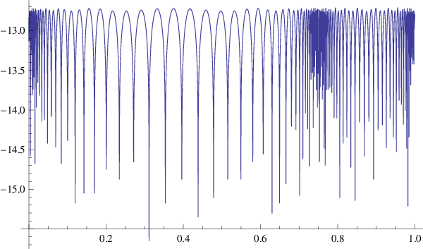
We apply the reduction algorithm using the approximation error δ=10−13\delta=10^{-13} (thus, the Cholesky decomposition algorithm 3 is truncated once the diagonal elements are smaller than ϵ​δ2\epsilon\delta^{2}, where ϵ\epsilon denotes the machine roundoff). As explained in Remark 4, Algorithms 2 and 3 are modified to accurately compute the partial Cholesky decomposition for poles in the form γj=e−τj\gamma_{j}=e^{-\tau_{j}}. After applying the reduction algorithm with approximation error δ=10−13\delta=10^{-13}, the resulting rational approximation contains 9292 pairs of conjugate-reciprocal poles (i.e., about 4646 poles per singularity). The resulting error is shown in Figure 3.1.

We note that the only step of the reduction procedure where quadruple precision is used is in computing the residues βj\beta_{j} (see Step 33 of Section 2.1). However, using the techniques described in the background Section 7.2 to factor the m×mm\times m Cauchy matrix, this step takes only 𝒪⁡(m2)\mathcal{O}\left(m^{2}\right) operations, and so does not impact the overall speed of the algorithm (recall that mm denotes the number of reduced poles).

Refer to caption
Refer to caption

(a) (b)

Figure 3.1. (a) Error of the rational approximation to f⁡(x)f\left(x\right) in (3.5). (b) A zoom on a neighbourhood around one of the singularities x∈(3/4−10−12,3/4+10−12)x\in\left(3/4-10^{-12},3/4+10^{-12}\right).

We find that the exponents, ηi\eta_{i}, of the near optimal poles ζi=exp⁡(−ηi)\zeta_{i}=\exp\left(-\eta_{i}\right) are computed with high relative accuracy, i.e.,

|Re​(ηi)−Re​(ηi^)|≤|Re​(ηi)|​δ1,|ηi−ηi^|≤|ηi|​δ2,\left|\text{Re}\left(\eta_{i}\right)-\text{Re}\left(\widehat{\eta_{i}}\right)\right|\leq\left|\text{Re}\left(\eta_{i}\right)\right|\delta_{1},\,\,\,\,\left|\eta_{i}-\widehat{\eta_{i}}\right|\leq\left|\eta_{i}\right|\delta_{2},

where δ1≤1.48×10⁻¹³\delta_{1}\leq 1.48\times 10^{-13} and δ2≤14.87×10⁻¹³\delta_{2}\leq 14.87\times 10^{-13}. As a gauge we used the poles ζi\zeta_{i} obtained in MathematicaT​M\,{}^{TM} via extended precision arithmetic. We note that the real parts of some of the exponents ηi\eta_{i} are of size |Re​(ηi)|≈10−12\left|\text{Re}\left(\eta_{i}\right)\right|\approx 10^{-12}.

3.2. Solving viscous Burgers’ equation

In [27] we use the reduction algorithm to solve viscous Burgers’ equation,

(3.6) ut−u​ux=ν​ux​x,u⁡(x,0)=u0​(x),u⁡(0,t)=u⁡(1,t),x∈[0,1],t≥0.u_{t}-uu_{x}=\nu u_{xx},\,\,\,u(x,0)=u_{0}(x),\,\,\,u(0,t)=u(1,t),\,\,\,x\in[0,1],\,\,\,t\geq 0.

The solution of this equation develops a shock (or a sharp transition) on an interval of size 𝒪⁡(ν)\mathcal{O}\left(\nu\right). We approximate solutions to (3.6) using rational functions of the form

u⁡(x,t)=∑j=1M0αj​(t)e−2​π​i​x−γj​(t)+∑j=1M0αj​(t)¯e2​π​i​x−γj​(t)¯+α0.u\left(x,t\right)=\sum_{j=1}^{M_{0}}\frac{\alpha_{j}\left(t\right)}{e^{-2\pi ix}-\gamma_{j}\left(t\right)}+\sum_{j=1}^{M_{0}}\frac{\overline{\alpha_{j}\left(t\right)}}{e^{2\pi ix}-\overline{\gamma_{j}\left(t\right)}}+\alpha_{0}.

The key idea is to develop a numerical calculus using the reduction algorithm. Although operators such as multiplication and convolution increase the number of poles in the representation, the reduction algorithm is employed at each stage to keep the number of poles near optimally small. Overall, about 10610^{6} applications of the reduction algorithm were employed to compute the solutions illustrated below, thus confirming its robustness and efficiency.

Figure 3.2 shows the computed solutions u⁡(x,ht​j)u(x,h_{t}j) to (3.6), with the viscosity ν=10−5\nu=10^{-5}, the step size hth_{t} and the initial condition u0​(x)=sin⁡(2​π​x)+1/2​sin⁡(4​π​x)u_{0}(x)=\sin(2\pi x)+1/2\sin(4\pi x). In our reduction procedure, we used the step size of ht=10−5h_{t}=10^{-5} and the error tolerance δ=10−9\delta=10^{-9} (to match the error of our time discretization). The solution u⁡(x,ht​j)u(x,h_{t}j) is shown for time steps tj=ht​jt_{j}=h_{t}j, j=102, 104, 2×10⁴, 3×10⁴, 5×10⁴j=10^{2},\,10^{4},\,2\times 10^{4},\,3\times 10^{4},\,5\times 10^{4}. We see that the solution u⁡(x,t)u(x,t) develops two moving sharp transition regions, which approach each other and eventually merge into a single one about x≈1/2x\approx 1/2. The rational representations of u⁡(x,tj)u(x,t_{j}) have 44, 1111, 3333, 2929, and 1919 pairs of conjugate-reciprocal poles, respectively. It also demonstrates that the transition regions of u⁡(x,t)u(x,t) occur within intervals of width of 𝒪⁡(ν)\mathcal{O}\left(\nu\right).

Refer to caption
Refer to caption
Figure 3.2. (a) Solution u⁡(x,tj)u(x,t_{j}), for tj=10−3t_{j}=10^{-3}, .1.1, .2.2, .3.3, and .5.5. (b) u⁡(x,tj)u(x,t_{j}) in the transition region (1/2−10−5,1/2+10−5)\left(1/2-10^{-5},1/2+10^{-5}\right), for tj=0.4t_{j}=0.4 (from [27]). These solutions are represented with 44, 1111, 3333, 2929, and 1919 pairs of conjugate-reciprocal poles.

4. Accuracy verification

We test the accuracy of Algorithm 4 on 500500 random Cauchy matrices, Ci​j=(αi​αj¯)/(1−γi​γj¯)C_{ij}=\left(\alpha_{i}\overline{\alpha_{j}}\right)/\left(1-\gamma_{i}\overline{\gamma_{j}}\right), i,j=1,…,120i,j=1,\dots,120. The complex poles γj=ρj​e2​π​i​ϕj\gamma_{j}=\rho_{j}e^{2\pi i\phi_{j}} and residues αj=ζj​e2​π​i​ψj\alpha_{j}=\zeta_{j}e^{2\pi i\psi_{j}} are generated by taking ρj\rho_{j}, ϕj\phi_{j}, and ψj\psi_{j} from the uniform distribution on (0,1)\left(0,1\right), and taking ζj\zeta_{j} from the uniform distribution on (0,10)\left(0,10\right). For each randomly generated matrix, we first compute, as a gauge, C¯​C=Z​Σ​Z−1\overline{C}C=Z\Sigma Z^{-1} using the in-built MathematicaT​M\,{}^{TM} eigenvalue solver with 300300 digits of precision, and compare the result with Z^\widehat{Z} and Σ^\widehat{\Sigma} computed via Algorithm 4 using standard double precision. We then evaluate the maximum relative error in the con-eigenvalues λj=Σj​j\lambda_{j}=\Sigma_{jj}, maxj⁡|λj−λj^|/|λj|\max_{j}\left|\lambda_{j}-\widehat{\lambda_{j}}\right|/\left|\lambda_{j}\right|, and the maximum error in the computed con-eigenvectors, maxj‖Z(:,j)−Z^(:,j)‖2/‖Z(:,j)‖2\max_{j}\left\|Z\left(:,j\right)-\widehat{Z}\left(:,j\right)\right\|_{2}/\left\|Z\left(:,j\right)\right\|_{2}. We first scale Z^(:,j)\widehat{Z}\left(:,j\right) by the complex-valued constant Z⁡(i0,j)/Z^​(i0,j)Z\left(i_{0},j\right)/\widehat{Z}\left(i_{0},j\right), i0=max1≤i≤n⁡|Z⁡(i,j)|i_{0}=\max_{1\leq i\leq n}\left|Z\left(i,j\right)\right|, since Z(:,j)Z\left(:,j\right) and Z^(:,j)\widehat{Z}\left(:,j\right) are defined only up to an arbitrary complex-valued factor.

Figures 4.1 and 4.2 summarize the result of a typical run. Figure 4.1(a) shows the distribution of the poles γj\gamma_{j} inside the unit disk and Figure 4.1(b) displays log10⁡λj2\log_{10}\lambda_{j}^{2} as a function of the index jj. Figures 4.2(a) 4.2(b) show the relative errors in the con-eigenvalues |λj−λj^|/|λj|\left|\lambda_{j}-\widehat{\lambda_{j}}\right|/\left|\lambda_{j}\right| and the normalized con-eigenvectors ‖zj−zj^‖2/‖zj‖2\left\|z_{j}-\widehat{z_{j}}\right\|_{2}/\left\|z_{j}\right\|_{2}, both as functions of the index jj.

(a) Refer to caption (b) Refer to caption

Figure 4.1. (a) Distribution of poles γj\gamma_{j} determining Cauchy matrix CC in a typical run. (b) Exponential decay of the eigenvalues λj2\lambda_{j}^{2} of C¯​C\overline{C}C as a function of the index jj using log10\log_{10} scale.

(a) Refer to caption (b)Refer to caption

Figure 4.2. (a) Relative error in the jjth con-eigenvalue, |λj−λj^|/|λj|\left|\lambda_{j}-\widehat{\lambda_{j}}\right|/\left|\lambda_{j}\right|, as a function of the index jj. (b) The error in the jjth con-eigenvector, ‖zj−zj^‖2/‖zj‖2\left\|z_{j}-\widehat{z_{j}}\right\|_{2}/\left\|z_{j}\right\|_{2}, zj=Z(:,j)z_{j}=Z\left(:,j\right), as a function of the index jj.

In Figures 4.3 and 4.4 for each of the 500500 random Cauchy matrices, we plot the error in the computed con-eigenvalues |λj^−λj|/|λj|\left|\widehat{\lambda_{j}}-\lambda_{j}\right|/\left|\lambda_{j}\right| and con-eigenvectors ‖zj^−zj‖2/‖zj‖2\left\|\widehat{z_{j}}-z_{j}\right\|_{2}/\left\|z_{j}\right\|_{2}for j=1,40,80,120j=1,40,80,120 (note the exponential decay of λj\lambda_{j}). We see that the con-eigenvalues and the con-eigenvectors are computed with nearly full precision for all the Cauchy matrices. In fact, the largest errors |λj^−λj|/|λj|\left|\widehat{\lambda_{j}}-\lambda_{j}\right|/\left|\lambda_{j}\right| and ‖zj^−zj‖2/‖zj‖2\left\|\widehat{z_{j}}-z_{j}\right\|_{2}/\left\|z_{j}\right\|_{2} in the computed con-eigenvalues and con-eigenvectors, for any of the 500500 Cauchy matrices and any 1≤j≤n1\leq j\leq n, are 5.13×10−125.13\times 10^{-12} and 5.35×10−125.35\times 10^{-12}.

(a) Refer to caption (b) Refer to caption

(c) Refer to caption (d) Refer to caption

Figure 4.3. Relative error in the computed con-eigenvalues, |λj^−λj|/|λj|\left|\widehat{\lambda_{j}}-\lambda_{j}\right|/\left|\lambda_{j}\right|, for j=1,40,80,120j=1,40,80,120 ((a), (b), (c), and (d), respectively), plotted for each of the 500500 random Cauchy matrices.

(a) Refer to caption (b) Refer to caption

(c) Refer to caption (d) Refer to caption

Figure 4.4. Relative error in the computed con-eigenvectors, ‖zj^−zj‖2/‖zj‖2\|\widehat{z_{j}}-z_{j}\|_{2}/\|z_{j}\|_{2}, for j=1,40,80,120j=1,40,80,120 ((a), (b), (c), and (d), respectively), plotted for each of the 500500 random Cauchy matrices.

5. Accuracy and perturbation theory

We show that Algorithm 4 of the previous section achieves high relative accuracy. We also demonstrate that small perturbations of aia_{i}, bjb_{j}, xix_{i}, and yjy_{j} determining CC lead to small relative perturbations of the con-eigenvalues and small perturbations of the angles between subspaces spanned by the con-eigenvectors, as long as the parameters xix_{i} and yjy_{j} are not too close in a relative sense.

For two (complex) floating point numbers xx and yy, we denote by fl​(x⊙y)\text{fl}\left(x\odot y\right) the result of applying the operation x⊙yx\odot y in floating point arithmetic, where ⊙\odot is one of the four basic operations, ⊙∈{+,−,×,÷}\odot\in\left\{+,-,\times,\div\right\}. We use that fl​(x⊙y)=(x⊙y)​(1+δ)\text{fl}\left(x\odot y\right)=\left(x\odot y\right)\left(1+\delta\right), where |δ|≤c​ϵ+𝒪⁡(ϵ2)\left|\delta\right|\leq c\epsilon+\mathcal{O}\left(\epsilon^{2}\right), ϵ\epsilon denote the machine round-off, and cc is a small constant (cf. [29]). We will also abuse notation by letting fl​(X​Y)\text{fl}\left(XY\right) denote the result of multiplying matrices XX and YY in floating point arithmetic. Finally, throughout this paper the notation ‖⋅‖\left\|\cdot\right\| always denotes the Frobenius norm.

In Theorems 5-7 below we always assume that the con-eigenvalues are simple, although this is not a crucial restriction. In the statements and proofs of these theorems, the implicit constant factor implied by the notation 𝒪⁡(η)\mathcal{O}\left(\eta\right) and 𝒪⁡(ϵ)\mathcal{O}\left(\epsilon\right) (here ϵ,η≪1\epsilon,\eta\ll 1) depends only on the size nn of the matrix CC. We also use the notation 𝒪⁡(1)\mathcal{O}\left(1\right) to denote a quantity that depends only on the size nn. We note that all these implicit constants may be tracked more carefully and are modest-sized functions of nn.

The bounds in the theorems below depend on the Cholesky factors in the decomposition C=(P​L)​D2​(P​L)∗C=\left(PL\right)D^{2}\left(PL\right)^{*}. In particular, let B=LT​LB=L^{\text{T}}L, and consider the (symmetric) LU factorization B=LB​LBTB=L_{B}L_{B}^{\text{T}}, where LBL_{B} is unit lower triangular. Then the estimates in Theorems 5 - 7 depend on the quantities

(5.1) μ0​(LB)\displaystyle\mu_{0}\left(L_{B}\right) =\displaystyle= ‖LB−1‖2​κ​(LB),\displaystyle\left\|L_{B}^{-1}\right\|^{2}\kappa\left(L_{B}\right),
μ1​(LB)\displaystyle\mu_{1}\left(L_{B}\right) =\displaystyle= max⁡{‖LB−1‖2,‖LB‖2}​κ​(LB),\displaystyle\max\left\{\left\|L_{B}^{-1}\right\|^{2},\left\|L_{B}\right\|^{2}\right\}\kappa\left(L_{B}\right),
μ2​(LB)\displaystyle\mu_{2}\left(L_{B}\right) =\displaystyle= ‖LB−1‖2​μ1​(LB)​κ3​(LB),\displaystyle\left\|L_{B}^{-1}\right\|^{2}\mu_{1}\left(L_{B}\right)\kappa^{3}\left(L_{B}\right),

where the condition number κ⁡(LB)=‖LB‖​‖LB−1‖\kappa\left(L_{B}\right)=\left\|L_{B}\right\|\left\|L_{B}^{-1}\right\| is not too large if BB and its nn leading principal submatrices are well-conditioned. The estimates in Theorems 6-7 also depend on

(5.2) μ3​(LB)=‖L−1‖​(ρ​μ​ψ​μ2​(LB)+ν​κ3​(LB)),\mu_{3}\left(L_{B}\right)=\left\|L^{-1}\right\|\left(\rho\mu\psi\mu_{2}\left(L_{B}\right)+\nu\kappa^{3}\left(L_{B}\right)\right),

where ρ\rho, μ\mu, and ψ\psi are “pivot growth” factors associated with the QR factorization (see Section 7.3), and the factor ν\nu is associated with the one-sided Jacobi algorithm (see (7.13)).

Remark.

There are simple formulas for Li​jL_{ij} and (L−1)i​j\left(L^{-1}\right)_{ij} ([10]) in terms of the parameters aia_{i}, bjb_{j}, xix_{i} and yjy_{j} defining the Cauchy matrix CC, and it is possible that the bounds below may be improved by using this additional structure.

Theorem 5.

Suppose that the parameters defining the positive-definite Cauchy matrix C=C⁡(a,b,x,y)C=C(a,b,x,y) are perturbed to a~=a+δ​a\tilde{a}=a+\delta a, b~=b+δ​b\tilde{b}=b+\delta b, x=x+δ​xx=x+\delta x, and y=y+δ​yy=y+\delta y. Let us define

η=(1/η1+1/η2+1/η3)​max⁡{‖δ​a‖∞,‖δ​b‖∞,‖δ​x‖∞,‖δ​y‖∞},\eta=\left(1/\eta_{1}+1/\eta_{2}+1/\eta_{3}\right)\max\left\{\left\|\delta a\right\|_{\infty},\left\|\delta b\right\|_{\infty},\left\|\delta x\right\|_{\infty},\left\|\delta y\right\|_{\infty}\right\},

where

η1=mini≠j⁡|xi−xj||xj|+|xi|,η2=mini≠j⁡|yi−yj||yj|+|yi|,η3=mini≠j⁡|xi+yj||xi|+|yj|.\eta_{1}=\min_{i\neq j}\frac{\left|x_{i}-x_{j}\right|}{\left|x_{j}\right|+\left|x_{i}\right|},\,\,\,\,\eta_{2}=\min_{i\neq j}\frac{\left|y_{i}-y_{j}\right|}{\left|y_{j}\right|+\left|y_{i}\right|},\,\,\,\,\eta_{3}=\min_{i\neq j}\frac{\left|x_{i}+y_{j}\right|}{\left|x_{i}\right|+\left|y_{j}\right|}.

Let C=L​D​L∗C=LDL^{*} denote the Cholesky factorization of CC, and let C~=C⁡(a~,b~,x~,y~)\widetilde{C}=C(\widetilde{a},\widetilde{b},\widetilde{x},\widetilde{y}) denote the Cauchy matrix corresponding to the perturbed parameters. Finally, let ziz_{i}, z~i\widetilde{z}_{i} denote the con-eigenvectors of CC and C~\widetilde{C}, corresponding to con-eigenvalues λi\lambda_{i} and λi~\widetilde{\lambda_{i}} .

Then the relative difference in the con-eigenvalues λi\lambda_{i} and λi~\widetilde{\lambda_{i}} is bounded as

|λi−λi~λi|≤μ0​(LB)​𝒪​(η),\left|\frac{\lambda_{i}-\widetilde{\lambda_{i}}}{\lambda_{i}}\right|\leq\mu_{0}\left(L_{B}\right)\mathcal{O}\left(\eta\right),

and the acute angle between the con-eigenvectors ziz_{i} and z~i\widetilde{z}_{i} is bounded by

sin⁡(∠​zi,zi~)≤κ⁡(L)​(μ2​(LB)relgapi+μ0​(LB)​μ1​(LB))​𝒪​(η).\sin\left(\angle z_{i},\widetilde{z_{i}}\right)\leq\kappa\left(L\right)\left(\frac{\mu_{2}\left(L_{B}\right)}{\text{relgap}{}_{i}}+\mu_{0}\left(L_{B}\right)\mu_{1}\left(L_{B}\right)\right)\mathcal{O}\left(\eta\right).

Here μ0​(LB)\mu_{0}\left(L_{B}\right), μ1​(LB)\mu_{1}\left(L_{B}\right) and μ2​(LB)\mu_{2}\left(L_{B}\right) are defined in (5.1), and

relgapi=minj≠i⁡|λi−λj||λi|+|λj|.\mbox{relgap}_{i}=\min_{j\neq i}\frac{\left|\lambda_{i}-\lambda_{j}\right|}{\left|\lambda_{i}\right|+\left|\lambda_{j}\right|}.

Next we state

Theorem 6.

Suppose that Algorithm 4 is used to compute the full con-eigenvalue decomposition of a positive-definite Cauchy matrix CC. Suppose also that CC has the Cholesky factorization C=(P​L)​D2​(P​L)∗C=\left(PL\right)D^{2}\left(PL\right)^{*}, where PP is the permutation matrix that encodes complete pivoting.

Then the relative error between the computed con-eigenvalue λi^\widehat{\lambda_{i}} and the exact λi\lambda_{i} is bounded as

|λi^−λi||λi|≤(ρ​μ​ψ​μ0​(LB)+ν)​𝒪​(ϵ),\frac{\left|\widehat{\lambda_{i}}-\lambda_{i}\right|}{\left|\lambda_{i}\right|}\leq\left(\rho\mu\psi\mu_{0}\left(L_{B}\right)+\nu\right)\mathcal{O}\left(\epsilon\right),

where ρ\rho, μ\mu, and ψ\psi are “pivot growth” factors associated with the QR factorization (see Section 7.3), and the factor ν\nu is associated with the one-sided Jacobi algorithm (see (7.13)).

Letting ziz_{i}, zi^\widehat{z_{i}} denote exact and computed con-eigenvectors of CC, the acute angle between ziz_{i} and zi^\widehat{z_{i}} then satisfies

sin⁡(∠​zi^,zi)≤κ⁡(L)​(μ3​(LB)relgapi+‖L−1‖2​κ3​(LB))​𝒪​(ϵ),\sin\left(\angle\widehat{z_{i}},z_{i}\right)\leq\kappa\left(L\right)\left(\frac{\mu_{3}\left(L_{B}\right)}{\text{relgap}{}_{i}}+\left\|L^{-1}\right\|^{2}\kappa^{3}\left(L_{B}\right)\right)\mathcal{O}\left(\epsilon\right),

where relgapi\mbox{relgap}_{i} is defined as in Theorem 5 and μ3​(LB)\mu_{3}\left(L_{B}\right) is defined in 5.2.

Theorem 7.

Suppose Algorithm 4 is used to compute mm approximate con-eigenvalues and con-eigenvectors of a positive-definite Cauchy matrix CC. Suppose also that CC has the Cholesky factorization C=(P​L)​D2​(P​L)∗C=\left(PL\right)D^{2}\left(PL\right)^{*}, where PP is the permutation matrix that encodes complete pivoting. Assuming that Dm​m2≤λi​ϵD_{mm}^{2}\leq\lambda_{i}\epsilon for some 1≤i≤m1\leq i\leq m, the following error bound holds for the computed con-eigenvalue λi^\widehat{\lambda_{i}},

|λi^−λi||λi|≤(ρ​μ​ψ​μ0​(LB)+ν+‖C‖​μ12​(LB))​𝒪​(ϵ),\frac{\left|\widehat{\lambda_{i}}-\lambda_{i}\right|}{\left|\lambda_{i}\right|}\leq\left(\rho\mu\psi\mu_{0}\left(L_{B}\right)+\nu+\left\|C\right\|\mu_{1}^{2}\left(L_{B}\right)\right)\mathcal{O}\left(\epsilon\right),

and the acute angle between ziz_{i} and zi^\widehat{z_{i}} is bounded by

sin⁡(∠​zi^,zi)≤κ⁡(L)​(μ3​(LB)+‖C‖​μ12​(LB)relgapi+‖L−1‖2​κ3​(LB))​𝒪​(ϵ).\sin\left(\angle\widehat{z_{i}},z_{i}\right)\leq\kappa\left(L\right)\left(\frac{\mu_{3}\left(L_{B}\right)+\left\|C\right\|\mu_{1}^{2}\left(L_{B}\right)}{\text{relgap}{}_{i}}+\left\|L^{-1}\right\|^{2}\kappa^{3}\left(L_{B}\right)\right)\mathcal{O}\left(\epsilon\right).

In the above estimates, ρ\rho, μ\mu, and ψ\psi are “pivot growth” factors associated with the QR factorization (see Section 7.3), and the factor ν\nu is associated with the one-sided Jacobi algorithm (see (7.13)).

Remark 8.

We note that the constants in the theorems above are significantly more pessimistic than we actually observe in numerical experiments. Indeed, while the bounds on the con-eigenvectors depend only on the well-conditioned matrices κ⁡(LB)\kappa\left(L_{B}\right) and k⁡(L)k\left(L\right) (and, in particular, are independent of the exponentially decaying diagonal matrix DD), they still scale like κ9\kappa^{9}, where κ=max⁡{κ⁡(LB),κ⁡(L)}\kappa=\max\left\{\kappa\left(L_{B}\right),\kappa\left(L\right)\right\}; the bounds on the con-eigenvalues are better—they scale like κ3\kappa^{3}. However, in practice Algorithm 4 achieves nearly full precision for all the con-eigenvalues and con-eigenvectors. While it is likely that better estimates can be obtained, those presented here elucidate the basic mechanism behind the high accuracy that we observe in our experiments.

5.1. Perturbation theorem

In this section, we prove Theorem 5. We start by formulating several preliminary results. Lemma 9 describes how perturbations of the vectors aa, bb, xx, and yy defining the Cauchy matrix C=C⁡(a,b,x,y)C=C(a,b,x,y) change the factors LL and DD in the Cholesky decomposition C=L​D​L∗C=LDL^{*} (see [15] for a proof).

Lemma 9.

Suppose the data defining the Cauchy matrix C=C⁡(a,b,x,y)C=C(a,b,x,y) is perturbed to a~=a+δ​a\tilde{a}=a+\delta a, b~=b+δ​b\tilde{b}=b+\delta b, x=x+δ​xx=x+\delta x, and y=y+δ​yy=y+\delta y. Let us define

η=(1/η1+1/η2+1/η3)​max⁡{‖δ​a‖∞,‖δ​b‖∞,‖δ​x‖∞,‖δ​y‖∞},\eta=\left(1/\eta_{1}+1/\eta_{2}+1/\eta_{3}\right)\max\left\{\left\|\delta a\right\|_{\infty},\left\|\delta b\right\|_{\infty},\left\|\delta x\right\|_{\infty},\left\|\delta y\right\|_{\infty}\right\},

where

η1=mini≠j⁡|xi−xj||xj|+|xi|,η2=mini≠j⁡|yi−yj||yj|+|yi|,η3=mini≠j⁡|xi+yj||xi|+|yj|.\eta_{1}=\min_{i\neq j}\frac{\left|x_{i}-x_{j}\right|}{\left|x_{j}\right|+\left|x_{i}\right|},\,\,\,\,\eta_{2}=\min_{i\neq j}\frac{\left|y_{i}-y_{j}\right|}{\left|y_{j}\right|+\left|y_{i}\right|},\,\,\,\,\eta_{3}=\min_{i\neq j}\frac{\left|x_{i}+y_{j}\right|}{\left|x_{i}\right|+\left|y_{j}\right|}.

Then C=C⁡(a,b,x,y)C=C(a,b,x,y) and C~=C~​(a~,b~,x~,y~)\widetilde{C}=\widetilde{C}(\widetilde{a},\widetilde{b},\widetilde{x},\widetilde{y}) have Cholesky factorizations C=L​D​L∗C=LDL^{*} and C~=L~​D~​L~∗\widetilde{C}=\widetilde{L}\widetilde{D}\widetilde{L}^{*}, where LL, L~\widetilde{L} are unit lower triangular matrices, DD, D~\widetilde{D} are diagonal matrices with positive entries, and

|Li​j−L^i​j|=|Li​j|​𝒪​(η),|Di​i−Di​i^|=|Di​i|​𝒪​(η).\left|L_{ij}-\widehat{L}_{ij}\right|=\left|L_{ij}\right|\mathcal{O}\left(\eta\right),\,\,\,\,\left|D_{ii}-\widehat{D_{ii}}\right|=\left|D_{ii}\right|\mathcal{O}\left(\eta\right).

We now state the main result needed to prove Theorem 5. Proposition 10 considers how a perturbation B+δ​BB+\delta B in D​B​DDBD affects the singular vectors. It turns out that, if all the principal minors of BB are well-conditioned, then the errors in the perturbed singular vectors are graded,

|vi​(j)−v~i​(j)|∼min⁡{Dj​jΣi​i,Σi​iDj​j}​𝒪​(‖δ​B‖).\left|v_{i}(j)-\widetilde{v}_{i}(j)\right|\sim\min\left\{\frac{D_{jj}}{\sqrt{\Sigma_{ii}}},\frac{\sqrt{\Sigma_{ii}}}{D_{jj}}\right\}\mathcal{O}\left(\left\|\delta B\right\|\right).

The proof uses techniques developed in [4], [20], and [34].

Proposition 10.

Suppose that G=D​B​DG=DBD and G~=D⁡(B+δ​B)​D\widetilde{G}=D\left(B+\delta B\right)D, where BB is complex symmetric (B=BTB=B^{\text{T}}) and non-singular, and DD is a diagonal matrix with positive, decreasing diagonal elements. Assume also that BB has the LU decomposition B=LB​LBTB=L_{B}L_{B}^{\text{T}}.

Then the iith singular values Σi​i\Sigma_{ii} and Σi​i~\widetilde{\Sigma_{ii}} of GG and G~\widetilde{G} satisfy

|Σi​i−Σi​i~Σi​i|≤μ0​(LB)​𝒪​(‖δ​B‖),\left|\frac{\Sigma_{ii}-\widetilde{\Sigma_{ii}}}{\Sigma_{ii}}\right|\leq\mu_{0}\left(L_{B}\right)\mathcal{O}\left(\left\|\delta B\right\|\right),

where μ0​(LB)\mu_{0}\left(L_{B}\right) is defined in 5.1. The iith (left or right) singular vectors uiu_{i} and u~i\widetilde{u}_{i} of GG and G~\widetilde{G}, corresponding to (simple) singular values Σi​i\Sigma_{ii} and Σi​i~\widetilde{\Sigma_{ii}}, may be chosen so that

|ui​(j)|≤μ1​(LB)​min⁡{Dj​jΣi​i1/2,Σi​i1/2Dj​j},\left|u_{i}(j)\right|\leq\mu_{1}\left(L_{B}\right)\min\left\{\frac{D_{jj}}{\Sigma_{ii}^{1/2}},\frac{\Sigma_{ii}^{1/2}}{D_{jj}}\right\},

and

|ui​(j)−u~i​(j)|≤μ2​(LB)​min⁡{Dj​jΣi​i1/2,Σi​i1/2Dj​j}​𝒪​(‖δ​B‖),\left|u_{i}(j)-\widetilde{u}_{i}(j)\right|\leq\mu_{2}\left(L_{B}\right)\min\left\{\frac{D_{jj}}{\Sigma_{ii}^{1/2}},\frac{\Sigma_{ii}^{1/2}}{D_{jj}}\right\}\mathcal{O}\left(\left\|\delta B\right\|\right),

where μ1​(LB)\mu_{1}\left(L_{B}\right) and μ2​(LB)\mu_{2}\left(L_{B}\right) are defined in 5.1. Finally, we have the following norm-wise bounds,

(5.3) ‖B‖1/2≤‖D​uiΣi​i1/2‖,‖B−1‖−1/2≤‖D−1uiΣi​i1/2‖,\left\|B\right\|^{1/2}\leq\left\|\frac{Du_{i}}{\Sigma_{ii}^{1/2}}\right\|,\,\,\,\left\|B^{-1}\right\|^{-1/2}\leq\left\|D^{-1}u_{i}\Sigma_{ii}^{1/2}\right\|,

where μ0​(LB)\mu_{0}\left(L_{B}\right) is defined in 5.1.

Proof.

See the Appendix for proofs of the component-wise bounds on the left singular vectors. The bound on the relative difference |Σi​i−Σi​i~|/Σi​i\left|\Sigma_{ii}-\widetilde{\Sigma_{ii}}\right|/\Sigma_{ii} is proven in [17].

We now prove the norm-wise bound on D​ui/Σi​i1/2Du_{i}/\Sigma_{ii}^{1/2}. To do so, note that D​B​DDBD has the SVD D​B​D=U​Σ​UTDBD=U\Sigma U^{\text{T}}, since BB is complex symmetric (i.e., BB has a Takagi factorization). Now suppose that D​B​D​ui¯=Σi​i​uiDBD\overline{u_{i}}=\Sigma_{ii}u_{i}. Then the bound for D​ui/Σi​i1/2Du_{i}/\Sigma_{ii}^{1/2} follows from

Σi​i=|(D​B​D​ui¯,ui)|=|(B​D​ui¯,D​ui)|≤‖B‖​‖D​ui‖2.\Sigma_{ii}=\left|\left(DBD\overline{u_{i}},u_{i}\right)\right|=\left|\left(BD\overline{u_{i}},Du_{i}\right)\right|\leq\left\|B\right\|\left\|Du_{i}\right\|^{2}.

Similarly, note that D−1​B−1​D−1​ui=Σi​i−1​ui¯D^{-1}B^{-1}D^{-1}u_{i}=\Sigma_{ii}^{-1}\overline{u_{i}}. The bound for D−1​ui​Σi​i1/2D^{-1}u_{i}\Sigma_{ii}^{1/2} then follows from

Σi​i−1=|(D−1​B−1​D−1​ui,ui¯)|=|(B−1​D−1​ui,D−1​ui¯)|≤‖B−1‖​‖D−1​ui‖2.\Sigma_{ii}^{-1}=\left|\left(D^{-1}B^{-1}D^{-1}u_{i},\overline{u_{i}}\right)\right|=\left|\left(B^{-1}D^{-1}u_{i},D^{-1}\overline{u_{i}}\right)\right|\leq\left\|B^{-1}\right\|\left\|D^{-1}u_{i}\right\|^{2}.

∎

We now prove Theorem 5.

Proof.

Recall that the matrix ZZ of con-eigenvectors satisfies Z=PL¯(DV¯Σ−1/2)Z=P\overline{L}\left(D\overline{V}\Sigma^{-1/2}\right), where C=(P​L)​D2​(P​L)∗C=\left(PL\right)D^{2}\left(PL\right)^{*} is the Cholesky factorization of CC (with complete pivoting) and VV is the matrix of right singular vectors of G=D⁡(LT​L)​DG=D\left(L^{\text{T}}L\right)D. Let C~=(P​L~)​D~2​(P​L~)∗\widetilde{C}=\left(P\widetilde{L}\right)\widetilde{D}^{2}\left(P\widetilde{L}\right)^{*} denote the Cholesky factorization of C~\widetilde{C}. From Lemma 9 (see also [15]),

(5.4) ‖L−L~‖=‖L‖​𝒪​(η),|Di​i−Di​i~Di​i|=𝒪⁡(η).\left\|L-\widetilde{L}\right\|=\left\|L\right\|\mathcal{O}\left(\eta\right),\,\,\,\,\left|\frac{D_{ii}-\widetilde{D_{ii}}}{D_{ii}}\right|=\mathcal{O}\left(\eta\right).

Defining G~=D~​(L~T​L~)​D~\widetilde{G}=\widetilde{D}\left(\widetilde{L}^{\text{T}}\widetilde{L}\right)\widetilde{D}, the above bounds yield G~=D⁡(LT​L+E)​D\widetilde{G}=D\left(L^{\text{T}}L+E\right)D, where ‖E‖=𝒪⁡(η)\left\|E\right\|=\mathcal{O}\left(\eta\right) (since complete pivoting is used in the Cholesky factorization of CC, ‖L‖=𝒪⁡(1)\left\|L\right\|=\mathcal{O}\left(1\right)). Since the iith con-eigenvalue λi\lambda_{i} of CC is given by λi=Σi​i\lambda_{i}=\Sigma_{ii}, the estimate for the relative difference |(λi−λi~)/λi|\left|\left(\lambda_{i}-\widetilde{\lambda_{i}}\right)/\lambda_{i}\right| now follows from Proposition 10.

To derive bounds for the singular vectors, we apply Proposition 10 to G~=D⁡(LT​L+E)​D\widetilde{G}=D\left(L^{\text{T}}L+E\right)D. In particular, there exist right unit singular vectors v~i\widetilde{v}_{i} of G~\widetilde{G} and viv_{i} of GG such that

(5.5) |vi​(j)|≤μ1​(LB)​di​j​(D,Σ),\left|v_{i}(j)\right|\leq\mu_{1}\left(L_{B}\right)d_{ij}\left(D,\Sigma\right),

and

(5.6) |vi​(j)−v~i​(j)|≤di​j​(D,Σ)​(μ2​(LB)relgapi)​O​(‖E‖)≤di​j​(D,Σ)​μ2​(LB)relgapi​𝒪​(η),\left|v_{i}(j)-\widetilde{v}_{i}(j)\right|\leq d_{ij}\left(D,\Sigma\right)\left(\frac{\mu_{2}\left(L_{B}\right)}{\mbox{relgap}{}_{i}}\right)O\left(\left\|E\right\|\right)\leq d_{ij}\left(D,\Sigma\right)\frac{\mu_{2}\left(L_{B}\right)}{\mbox{relgap}{}_{i}}\mathcal{O}\left(\eta\right),

where

di​j​(D,Σ)=min⁡{Dj​jΣi​i1/2,Σi​i1/2Dj​j2}.d_{ij}\left(D,\Sigma\right)=\min\left\{\frac{D_{jj}}{\Sigma_{ii}^{1/2}},\frac{\Sigma_{ii}^{1/2}}{D_{jj}^{2}}\right\}.

Here μ1​(LB)\mu_{1}\left(L_{B}\right) and μ2​(LB)\mu_{2}\left(L_{B}\right) are defined in (5.1). Proposition 10 also shows that

(5.7) 1−μ0​(LB)​𝒪​(η)≤Σi​iΣi​i~≤1+μ0​(LB)​𝒪​(η).1-\mu_{0}\left(L_{B}\right)\mathcal{O}\left(\eta\right)\leq\frac{\Sigma_{ii}}{\widetilde{\Sigma_{ii}}}\leq 1+\mu_{0}\left(L_{B}\right)\mathcal{O}\left(\eta\right).

Finally, defining wi=D​vi/Σi​i1/2w_{i}=Dv_{i}/\Sigma_{ii}^{1/2} and w~i=D~​v~i/Σi​i~1/2\widetilde{w}_{i}=\widetilde{D}\widetilde{v}_{i}/\widetilde{\Sigma_{ii}}^{1/2}, we have

|wi​(j)−w~i​(j)|\displaystyle\left|w_{i}(j)-\widetilde{w}_{i}(j)\right| =\displaystyle= Dj​jΣi​i1/2​|vi​(j)−Dj​j~Dj​j​(Σi​iΣi​i~)1/2​v~i​(j)|\displaystyle\frac{D_{jj}}{\Sigma_{ii}^{1/2}}\left|v_{i}(j)-\frac{\widetilde{D_{jj}}}{D_{jj}}\left(\frac{\Sigma_{ii}}{\widetilde{\Sigma_{ii}}}\right)^{1/2}\widetilde{v}_{i}(j)\right|
≤\displaystyle\leq Dj​jΣi​i1/2​(|vi​(j)−v~i​(j)|+|vi​(j)|​μ0​(LB)​𝒪​(η))\displaystyle\frac{D_{jj}}{\Sigma_{ii}^{1/2}}\left(\left|v_{i}(j)-\widetilde{v}_{i}(j)\right|+\left|v_{i}(j)\right|\mu_{0}\left(L_{B}\right)\mathcal{O}\left(\eta\right)\right)
≤\displaystyle\leq (μ2​(LB)relgapi+μ0​(LB)​μ1​(LB))​𝒪​(η),\displaystyle\left(\frac{\mu_{2}\left(L_{B}\right)}{\mbox{relgap}{}_{i}}+\mu_{0}\left(L_{B}\right)\mu_{1}\left(L_{B}\right)\right)\mathcal{O}\left(\eta\right),

where we used (5.4) and (5.7) in the first inequality, and (5.5)-(5.6) in the last one.

Proposition 10 also implies that 1/‖wi‖≤σmax1/2​(LT​L)=𝒪⁡(1)1/\left\|w_{i}\right\|\leq\sigma_{\max}^{1/2}\left(L^{\text{T}}L\right)=\mathcal{O}\left(1\right) and 1/‖wi^‖≤𝒪⁡(1)1/\left\|\widehat{w_{i}}\right\|\leq\mathcal{O}\left(1\right) (since complete pivoting is used, ‖L‖=𝒪⁡(1)\left\|L\right\|=\mathcal{O}\left(1\right)). The proof now follows upon noting that the con-eigenvectors ziz_{i} and zi~\widetilde{z_{i}} satisfy zi=L​wiz_{i}=Lw_{i}, zi~=L~​wi~\widetilde{z_{i}}=\widetilde{L}\widetilde{w_{i}}, and using (5.4),

‖zi−zi~‖‖zi‖\displaystyle\frac{\left\|z_{i}-\widetilde{z_{i}}\right\|}{\left\|z_{i}\right\|} ≤\displaystyle\leq ‖L​wi−L​wi~‖‖L​wi‖+‖L‖​‖wi~‖‖L​wi~‖​𝒪​(η)\displaystyle\frac{\left\|Lw_{i}-L\widetilde{w_{i}}\right\|}{\left\|Lw_{i}\right\|}+\left\|L\right\|\frac{\left\|\widetilde{w_{i}}\right\|}{\left\|L\widetilde{w_{i}}\right\|}\mathcal{O}\left(\eta\right)
≤\displaystyle\leq ‖L‖​‖L−1‖​(‖wi−wi~‖‖wi‖+𝒪⁡(η))\displaystyle\left\|L\right\|\left\|L^{-1}\right\|\left(\frac{\left\|w_{i}-\widetilde{w_{i}}\right\|}{\left\|w_{i}\right\|}+\mathcal{O}\left(\eta\right)\right)
≤\displaystyle\leq κ⁡(L)​(μ2​(LB)relgapi+μ0​(LB)​μ1​(LB))​𝒪​(η).\displaystyle\kappa\left(L\right)\left(\frac{\mu_{2}\left(L_{B}\right)}{\mbox{relgap}{}_{i}}+\mu_{0}\left(L_{B}\right)\mu_{1}\left(L_{B}\right)\right)\mathcal{O}\left(\eta\right).

∎

5.2. Proof of Theorem 6 (high relative accuracy of Algorithm 4)

We now show that Algorithm 4 accurately computes the eigenvectors of C¯​C\overline{C}C (recall that C=(P​L)​D2​(P​L)∗C=\left(PL\right)D^{2}\left(PL\right)^{*}), as long as the nn leading principal minors of LT​LL^{T}L are well-conditioned and the relative gap between the eigenvalues is not too small.

Before proving Theorem 6, we first need several lemmas on graded matrices.

Lemma 11.

Let DD be a positive definite diagonal matrix with decreasing diagonal elements, and let LL and RR denote nonsingular lower and upper triangular matrices. Then

‖D​L​D−1‖≤‖L‖,‖(D​L​D−1)−1‖≤‖L−1‖,\left\|DLD^{-1}\right\|\leq\left\|L\right\|,\,\,\,\left\|\left(DLD^{-1}\right)^{-1}\right\|\leq\left\|L^{-1}\right\|,

and

‖D−1​R​D‖≤‖R‖,‖(D−1​R​D)−1‖≤‖R−1‖.\left\|D^{-1}RD\right\|\leq\left\|R\right\|,\,\,\,\left\|\left(D^{-1}RD\right)^{-1}\right\|\leq\left\|R^{-1}\right\|.
Proof.

Since the diagonal elements of DD are decreasing and LL is lower triangular,

|(D​L​D−1)i​j|≤Di​iDj​j​|Li​j|≤|Li​j|,\left|\left(DLD^{-1}\right)_{ij}\right|\leq\frac{D_{ii}}{D_{jj}}\left|L_{ij}\right|\leq\left|L_{ij}\right|,

and

|(D​L​D−1)i​j−1|≤Di​iDj​j​|(L−1)i​j|≤|(L−1)i​j|.\left|\left(DLD^{-1}\right)_{ij}^{-1}\right|\leq\frac{D_{ii}}{D_{jj}}\left|\left(L^{-1}\right)_{ij}\right|\leq\left|\left(L^{-1}\right)_{ij}\right|.

Since the Frobenius norm is absolute, the first two inequalities in Lemma 11 follow. The other two inequalities can be shown in a similar fashion. ∎

Lemma 12.

Let D>0D>0 denote a diagonal matrix with decreasing diagonal elements, and let BB denote a non-singular, complex symmetric matrix with LU factorization B=LB​LBTB=L_{B}L_{B}^{\text{T}}. Suppose that D​B​DDBD has the QR factorization Q​R=D​B​DQR=DBD. Then the upper triangular matrix R0=D−2​RR_{0}=D^{-2}R satisfies

‖D​R0​D−1‖≤‖LB‖2,‖D​R0−1​D−1‖≤‖LB−1‖2.\left\|DR_{0}D^{-1}\right\|\leq\left\|L_{B}\right\|^{2},\,\,\,\left\|DR_{0}^{-1}D^{-1}\right\|\leq\left\|L_{B}^{-1}\right\|^{2}.

Moreover, the iith left singular vector uiu_{i} of RR (corresponding to singular value Σi​i\Sigma_{ii}) satisfies

(5.8) ‖D−1uiΣi​i1/2‖≥‖B−1‖−1/2κ−1(LB).\left\|D^{-1}u_{i}\Sigma_{ii}^{1/2}\right\|\geq\left\|B^{-1}\right\|^{-1/2}\kappa^{-1}\left(L_{B}\right).
Proof.

First note D​B​D=(D​LB​D−1)​(D​LBT​D)DBD=\left(DL_{B}D^{-1}\right)\left(DL_{B}^{\text{T}}D\right). Now suppose that D​LB​D−1DL_{B}D^{-1} has the QR factorization Q1​R1=D​LB​D−1Q_{1}R_{1}=DL_{B}D^{-1}. Then Q1​(R1​D​LBT​D)=Q​RQ_{1}\left(R_{1}DL_{B}^{\text{T}}D\right)=QR. Since R1​D​LBT​DR_{1}DL_{B}^{\text{T}}D is upper triangular, there is a diagonal matrix Ω\Omega such that |Ωi​j|=1\left|\Omega_{ij}\right|=1, Q=Q1​Ω−1Q=Q_{1}\Omega^{-1}, and R=Ω​R1​D​LBT​DR=\Omega R_{1}DL_{B}^{\text{T}}D. Therefore, we have

R0=D−2​R=Ω​D−2​R1​D​LBT​D.R_{0}=D^{-2}R=\Omega D^{-2}R_{1}DL_{B}^{\text{T}}D.

It follows that D​R0​D−1=Ω⁡(D−1​R1​D)​LBTDR_{0}D^{-1}=\Omega\left(D^{-1}R_{1}D\right)L_{B}^{\text{T}}, and we obtain

‖D​R0​D−1‖\displaystyle\left\|DR_{0}D^{-1}\right\| =\displaystyle= ‖Ω⁡(D−1​R1​D)​LBT‖≤‖R1‖​‖LBT‖≤‖LB‖2.\displaystyle\left\|\Omega\left(D^{-1}R_{1}D\right)L_{B}^{\text{T}}\right\|\leq\left\|R_{1}\right\|\left\|L_{B}^{\text{T}}\right\|\leq\left\|L_{B}\right\|^{2}.

In the first inequality, we use Lemma 11, and in the last one we use ‖R1‖=‖D​LB​D−1‖\left\|R_{1}\right\|=\left\|DL_{B}D^{-1}\right\| and Lemma 11. Similarly, we have

‖D​R0−1​D−1‖\displaystyle\left\|DR_{0}^{-1}D^{-1}\right\| =\displaystyle= ‖(LBT)−1​(D−1​R1−1​D)​Ω−1‖≤‖R1−1‖​‖(LBT)−1‖≤‖LB−1‖2,\displaystyle\left\|\left(L_{B}^{\text{T}}\right)^{-1}\left(D^{-1}R_{1}^{-1}D\right)\Omega^{-1}\right\|\leq\left\|R_{1}^{-1}\right\|\left\|\left(L_{B}^{\text{T}}\right)^{-1}\right\|\leq\left\|L_{B}^{-1}\right\|^{2},

where we use Lemma 11 in the first inequality, and ‖R1−1‖=‖D​LB−1​D−1‖\left\|R_{1}^{-1}\right\|=\left\|DL_{B}^{-1}D^{-1}\right\| and Lemma 11 in the last one.

In order to prove the bound for D−1​ui​Σi​i1/2D^{-1}u_{i}\Sigma_{ii}^{1/2}, we first claim that ‖D−1​Q​D‖≤κ⁡(LB)\left\|D^{-1}QD\right\|\leq\kappa\left(L_{B}\right). Indeed, since Q1​R1=D​LB​D−1Q_{1}R_{1}=DL_{B}D^{-1} and Q=Q1​Ω−1Q=Q_{1}\Omega^{-1}, we have

‖D−1​Q​D‖\displaystyle\left\|D^{-1}QD\right\| =\displaystyle= ‖D−1​Q1​D‖=‖LB​(D−1​R1−1​D)‖\displaystyle\left\|D^{-1}Q_{1}D\right\|=\left\|L_{B}\left(D^{-1}R_{1}^{-1}D\right)\right\|
≤\displaystyle\leq ‖LB‖​‖D−1​R1−1​D‖\displaystyle\left\|L_{B}\right\|\left\|D^{-1}R_{1}^{-1}D\right\|
≤\displaystyle\leq ‖LB‖​‖R1−1‖≤‖LB‖​‖D​LB−1​D−1‖≤‖LB‖​‖LB−1‖.\displaystyle\left\|L_{B}\right\|\left\|R_{1}^{-1}\right\|\leq\left\|L_{B}\right\|\left\|DL_{B}^{-1}D^{-1}\right\|\leq\left\|L_{B}\right\|\left\|L_{B}^{-1}\right\|.

In the above string of inequalities, we use of Lemma 11 repeatedly.

Now, if RR has the SVD R=U​Σ​V∗R=U\Sigma V^{*}, then D−1​B−1​D−1D^{-1}B^{-1}D^{-1} has the SVD D−1​B−1​D−1=V​Σ−1​(Q​U)∗D^{-1}B^{-1}D^{-1}=V\Sigma^{-1}\left(QU\right)^{*} (recall that Q​R=D​B​DQR=DBD). Therefore, the left and right singular vectors uiu_{i} and viv_{i} of RR satisfy (D−1​B−1​D−1)​(Q​ui)=Σi​i−1​vi\left(D^{-1}B^{-1}D^{-1}\right)\left(Qu_{i}\right)=\Sigma_{ii}^{-1}v_{i}. Since BB is complex symmetric, we may also assume (without loss of generality) that Q​ui=vi¯Qu_{i}=\overline{v_{i}}. The bound on ‖D−1​ui​Σi​i1/2‖\left\|D^{-1}u_{i}\Sigma_{ii}^{1/2}\right\| now follows from

Σi​i−1\displaystyle\Sigma_{ii}^{-1} =\displaystyle= |(B−1​(D−1​vi¯),D−1​vi)|≤‖B−1‖​‖D−1​vi‖​‖D−1​vi¯‖\displaystyle\left|\left(B^{-1}\left(D^{-1}\overline{v_{i}}\right),D^{-1}v_{i}\right)\right|\leq\left\|B^{-1}\right\|\left\|D^{-1}v_{i}\right\|\left\|D^{-1}\overline{v_{i}}\right\|
=\displaystyle= ‖B−1‖​‖D−1​vi‖2=‖B−1‖​‖D−1​Q​ui‖2\displaystyle\left\|B^{-1}\right\|\left\|D^{-1}v_{i}\right\|^{2}=\left\|B^{-1}\right\|\left\|D^{-1}Qu_{i}\right\|^{2}
=\displaystyle= ‖B−1‖​‖(D−1​Q​D)​D−1​ui‖2\displaystyle\left\|B^{-1}\right\|\left\|\left(D^{-1}QD\right)D^{-1}u_{i}\right\|^{2}
≤\displaystyle\leq ‖B−1‖​κ2​(LB)​‖D−1​ui‖2.\displaystyle\left\|B^{-1}\right\|\kappa^{2}\left(L_{B}\right)\left\|D^{-1}u_{i}\right\|^{2}.

In the last inequality, we used the bound ‖D−1​Q​D‖≤κ⁡(LB)\left\|D^{-1}QD\right\|\leq\kappa\left(L_{B}\right), as shown in the previous paragraph.∎

Lemma 13.

Let D​B​DDBD, QQ, RR, and LBL_{B} be as in Lemma 12, and define R1=D−1​R​D−1R_{1}=D^{-1}RD^{-1}. Then κ⁡(R1)≤κ2​(LB)\kappa\left(R_{1}\right)\leq\kappa^{2}\left(L_{B}\right), and the iith right singular vector viv_{i} of RR (corresponding to singular value Σi​i\Sigma_{ii}) satisfies

DviΣi​i−1/2=R1−1(D−1uiΣi​i1/2),Dv_{i}\Sigma_{ii}^{-1/2}=R_{1}^{-1}\left(D^{-1}u_{i}\Sigma_{ii}^{1/2}\right),

where

‖R1‖≤‖LB‖2,‖R1−1‖≤‖LB−1‖2.\left\|R_{1}\right\|\leq\left\|L_{B}\right\|^{2},\,\,\,\left\|R_{1}^{-1}\right\|\leq\left\|L_{B}^{-1}\right\|^{2}.
Proof.

Define R0=D−2​RR_{0}=D^{-2}R and R1=D−1​R​D−1R_{1}=D^{-1}RD^{-1}. Then since R1=D​R0​D−1R_{1}=DR_{0}D^{-1}, the bounds for ‖R1‖\left\|R_{1}\right\| and ‖R1−1‖\left\|R_{1}^{-1}\right\| follow from Lemma 12. Using (2.6), we also have that

DviΣi​i−1/2\displaystyle Dv_{i}\Sigma_{ii}^{-1/2} =\displaystyle= D​R−1​ui​Σi​i1/2\displaystyle DR^{-1}u_{i}\Sigma_{ii}^{1/2}
=\displaystyle= (D​R0−1​D−1)​(D−1​ui​Σi​i1/2)\displaystyle\left(DR_{0}^{-1}D^{-1}\right)\left(D^{-1}u_{i}\Sigma_{ii}^{1/2}\right)
=\displaystyle= (D​R0​D−1)−1​(D−1​ui​Σi​i1/2)\displaystyle\left(DR_{0}D^{-1}\right)^{-1}\left(D^{-1}u_{i}\Sigma_{ii}^{1/2}\right)
=\displaystyle= R1−1​(D−1​ui​Σi​i1/2).\displaystyle R_{1}^{-1}\left(D^{-1}u_{i}\Sigma_{ii}^{1/2}\right).

∎

We now prove Theorem 6.

Proof.

First consider Step 11 of Algorithm 4. From [15], the computed Cholesky factors D^\widehat{D} and L^\widehat{L} of CC satisfy

(5.9) |Di​j−Di​j^|≤|Di​j|​𝒪​(ϵ),‖L−L^‖≤𝒪⁡(ϵ).\left|D_{ij}-\widehat{D_{ij}}\right|\leq\left|D_{ij}\right|\mathcal{O}\left(\epsilon\right),\,\,\,\,\left\|L-\widehat{L}\right\|\leq\mathcal{O}\left(\epsilon\right).

We now examine the error in applying Algorithm 1 to compute the con-eigenvectors and con-eigenvalues.

In Step 11 of Algorithm 1, the computed matrix G^\widehat{G} satisfies G^=fl​(D^​(L^T​L^)​D^)=D⁡(LT​L+E0)​D\widehat{G}=\text{fl}\left(\widehat{D}\left(\widehat{L}^{\text{T}}\widehat{L}\right)\widehat{D}\right)=D\left(L^{\text{T}}L+E_{0}\right)D, where ‖E0‖≤𝒪⁡(ϵ)\left\|E_{0}\right\|\leq\mathcal{O}\left(\epsilon\right) (recall that complete pivoting is used, so that ‖L‖=𝒪⁡(1)\left\|L\right\|=\mathcal{O}\left(1\right)).

In Step 22 of Algorithm 1, a computed upper triangular factor R^\widehat{R} of G^\widehat{G} is obtained using the Householder QR algorithm. By Theorem 17 in Section 7.3, there is an orthogonal matrix QQ such that

(5.10) Q​R^=D⁡(LT​L+E2)​D,Q\widehat{R}=D\left(L^{\text{T}}L+E_{2}\right)D,

where E2=E0+E1E_{2}=E_{0}+E_{1}, ‖E1‖≤ρ​μ​ψ​𝒪​(ϵ)\left\|E_{1}\right\|\leq\rho\mu\psi\mathcal{O}\left(\epsilon\right), and ρ\rho, μ\mu, and ψ\psi are “pivot growth factors” described in Section 7.3. Now suppose that LT​L+E2L^{\text{T}}L+E_{2} has an LU factorization LT​L+E2=LB~​UB~L^{\text{T}}L+E_{2}=\widetilde{L_{B}}\widetilde{U_{B}}. By Lemma 12, R0=D−2​R^R_{0}=D^{-2}\widehat{R} satisfies

(5.11) ‖D​R0​D−1‖≤‖LB‖2+𝒪⁡(ϵ),‖D​R0−1​D−1‖≤‖LB−1‖2+𝒪⁡(ϵ),\left\|DR_{0}D^{-1}\right\|\leq\left\|L_{B}\right\|^{2}+\mathcal{O}\left(\epsilon\right),\,\,\,\left\|DR_{0}^{-1}D^{-1}\right\|\leq\left\|L_{B}^{-1}\right\|^{2}+\mathcal{O}\left(\epsilon\right),

where we used that ‖LB‖=‖LB~‖+𝒪⁡(ϵ)\left\|L_{B}\right\|=\left\|\widetilde{L_{B}}\right\|+\mathcal{O}\left(\epsilon\right) and ‖LB−1‖=‖LB~−1‖+𝒪⁡(ϵ)\left\|L_{B}^{-1}\right\|=\left\|\widetilde{L_{B}}^{-1}\right\|+\mathcal{O}\left(\epsilon\right).

Step 33 of Algorithm 1 involves computing an approximate SVD R^≈Ul^​Σ^​Ur^∗\widehat{R}\approx\widehat{U_{l}}\widehat{\Sigma}\widehat{U_{r}}^{*} using the modified one-sided Jacobi algorithm, applied from the left. Note that, from (5.10), if R^\widehat{R} has the (exact) SVD R^=Ul​Σ​Ur∗\widehat{R}=U_{l}\Sigma U_{r}^{*}, then Q​UlQU_{l} and UrU_{r} are the matrices of left and right singular vectors of D⁡(LT​L+E2)​DD\left(L^{\text{T}}L+E_{2}\right)D. Moreover, if Σi​i~\widetilde{\Sigma_{ii}} denotes the exact singular value of R^\widehat{R} (and D⁡(LT​L+E2)​DD\left(L^{\text{T}}L+E_{2}\right)D), then Proposition 10 ensures that

|Σi​i~−Σi​i|Σi​i~≤μ0​(LB)​𝒪​(‖E2‖)≤ρ​μ​ψ​μ0​(LB)​𝒪​(ϵ).\frac{\left|\widetilde{\Sigma_{ii}}-\Sigma_{ii}\right|}{\widetilde{\Sigma_{ii}}}\leq\mu_{0}\left(L_{B}\right)\mathcal{O}\left(\left\|E_{2}\right\|\right)\leq\rho\mu\psi\mu_{0}\left(L_{B}\right)\mathcal{O}\left(\epsilon\right).

Now let Σi​i^\widehat{\Sigma_{ii}} denote the computed singular value of R^\widehat{R} obtained via the one-sided Jacobi algorithm. Then from Theorem 18 and the equality R^=D2​R0\widehat{R}=D^{2}R_{0}, we also have that

|Σi​i~−Σi​i^|Σi​i~≤ν0​𝒪​(ϵ).\frac{\left|\widetilde{\Sigma_{ii}}-\widehat{\Sigma_{ii}}\right|}{\widetilde{\Sigma_{ii}}}\leq\nu_{0}\mathcal{O}\left(\epsilon\right).

Combining the previous two inequalities yields the bound on the computed con-eigenvalues (recall that the exact and computed con-eigenvalues satisfy λi=Σi​i\lambda_{i}=\Sigma_{ii} and λi^=Σi​i^\widehat{\lambda_{i}}=\widehat{\Sigma_{ii}}).

Now let ui^\widehat{u_{i}} and Σ^i​i\widehat{\Sigma}_{ii} denote the iith computed left singular vector and singular value of R^\widehat{R}. Then by Theorem 18 and the equality R^=D2​R0\widehat{R}=D^{2}R_{0}, there is an exact left singular vector ui(1)u_{i}^{(1)} of R^\widehat{R}, corresponding to singular value Σ~i​i\widetilde{\Sigma}_{ii}, such that

(5.12) ‖D−1​(ui^−ui(1))​Σ~i​i1/2‖≤νrelgapi​𝒪​(ϵ),\left\|D^{-1}\left(\widehat{u_{i}}-u_{i}^{(1)}\right)\widetilde{\Sigma}_{ii}^{1/2}\right\|\leq\frac{\nu}{\mbox{relgap}_{i}}\mathcal{O}\left(\epsilon\right),

where ν\nu is described in Theorem 18 in Section 7.4 (see, in particular, (7.13)).

Now define R1=D−1​R^​D−1R_{1}=D^{-1}\widehat{R}D^{-1} and R1^=fl​(D^−1​R^​D^−1)\widehat{R_{1}}=\text{fl}\left(\widehat{D}^{-1}\widehat{R}\widehat{D}^{-1}\right). We show that the computed vector yi^≈R1^−1​(D^−1​ui^​Σ^i​i1/2)\widehat{y_{i}}\approx\widehat{R_{1}}^{-1}\left(\widehat{D}^{-1}\widehat{u_{i}}\widehat{\Sigma}_{ii}^{1/2}\right), obtained from Step 44 of Algorithm 1, is close to yi(1)=R1−1​(D−1​ui(1)​Σ~i​i1/2)y_{i}^{(1)}=R_{1}^{-1}\left(D^{-1}u_{i}^{(1)}\widetilde{\Sigma}_{ii}^{1/2}\right). In particular, Step 44 involves computing an approximation yi^\widehat{y_{i}} to the triangular system R1^​yi(0)=xi^\widehat{R_{1}}y_{i}^{(0)}=\widehat{x_{i}}, where xi^=fl​(D^−1​ui^​Σ^i​i1/2)\widehat{x_{i}}=\text{fl}\left(\widehat{D}^{-1}\widehat{u_{i}}\widehat{\Sigma}_{ii}^{1/2}\right) and

R1^=fl​(D^−1​R^​D^−1)=R1+δ​R1,‖δ​R1‖‖R1‖≤𝒪⁡(ϵ).\widehat{R_{1}}=\text{fl}\left(\widehat{D}^{-1}\widehat{R}\widehat{D}^{-1}\right)=R_{1}+\delta R_{1},\,\,\,\frac{\left\|\delta R_{1}\right\|}{\left\|R_{1}\right\|}\leq\mathcal{O}\left(\epsilon\right).

In the above inequality for ‖δ​R1‖\left\|\delta R_{1}\right\|, we used (5.9). We will also need the following expression for R1R_{1}, which follows from Lemma 12:

(5.13) R1=D​R0​D−1,κ⁡(R1)≤κ2​(LB)+𝒪⁡(ϵ).R_{1}=DR_{0}D^{-1},\,\,\,\kappa\left(R_{1}\right)\leq\kappa^{2}\left(L_{B}\right)+\mathcal{O}\left(\epsilon\right).

Now, recall that yi(1)y_{i}^{(1)} is the exact solution of R1​yi(1)=xiR_{1}y_{i}^{(1)}=x_{i}, xi=D−1​ui(1)​Σ~i​i1/2x_{i}=D^{-1}u_{i}^{(1)}\widetilde{\Sigma}_{ii}^{1/2}. Since yi^\widehat{y_{i}} is computed from the system R1^​yi(0)=xi^\widehat{R_{1}}y_{i}^{(0)}=\widehat{x_{i}} by backsubstitution, there is a matrix δ​R2\delta R_{2} such that ‖δ​R2‖/‖R2‖=𝒪⁡(ϵ)\left\|\delta R_{2}\right\|/\left\|R_{2}\right\|=\mathcal{O}\left(\epsilon\right) and (R1+δ​R2)​yi^=xi+(xi^−xi)\left(R_{1}+\delta R_{2}\right)\widehat{y_{i}}=x_{i}+\left(\widehat{x_{i}}-x_{i}\right). Therefore,

(5.14) ‖yi(1)−yi^‖‖yi(1)‖\displaystyle\frac{\left\|y_{i}^{(1)}-\widehat{y_{i}}\right\|}{\left\|y_{i}^{(1)}\right\|} ≤\displaystyle\leq κ⁡(R1)​(‖(xi^−xi)‖‖xi‖+𝒪⁡(ϵ))\displaystyle\kappa\left(R_{1}\right)\left(\frac{\left\|\left(\widehat{x_{i}}-x_{i}\right)\right\|}{\left\|x_{i}\right\|}+\mathcal{O}\left(\epsilon\right)\right)
≤\displaystyle\leq κ2​(LB)​(‖(xi^−xi)‖‖xi‖+𝒪⁡(ϵ)),\displaystyle\kappa^{2}\left(L_{B}\right)\left(\frac{\left\|\left(\widehat{x_{i}}-x_{i}\right)\right\|}{\left\|x_{i}\right\|}+\mathcal{O}\left(\epsilon\right)\right),

where we used (5.13) in the last inequality. To bound ‖(xi^−xi)‖\left\|\left(\widehat{x_{i}}-x_{i}\right)\right\|, we compute that

xi^​(j)\displaystyle\widehat{x_{i}}\left(j\right) =\displaystyle= fl​(D^j​j−1​ui^​(j)​Σ^i​i1/2)=D^j​j−1​ui^​(j)​Σ^i​i1/2​(1+𝒪⁡(ϵ))\displaystyle\text{fl}\left(\widehat{D}_{jj}^{-1}\widehat{u_{i}}\left(j\right)\widehat{\Sigma}_{ii}^{1/2}\right)=\widehat{D}_{jj}^{-1}\widehat{u_{i}}\left(j\right)\widehat{\Sigma}_{ii}^{1/2}\left(1+\mathcal{O}\left(\epsilon\right)\right)
=\displaystyle= Dj​j−1​ui^​(j)​Σ~i​i1/2​(Σ^i​iΣ~i​i)1/2​(1+𝒪⁡(ϵ))\displaystyle D_{jj}^{-1}\widehat{u_{i}}\left(j\right)\widetilde{\Sigma}_{ii}^{1/2}\left(\frac{\widehat{\Sigma}_{ii}}{\widetilde{\Sigma}_{ii}}\right)^{1/2}\left(1+\mathcal{O}\left(\epsilon\right)\right)
=\displaystyle= Dj​j−1​ui^​(j)​Σ~i​i1/2​(1+‖LB−1‖2​κ​(LB)​𝒪​(ϵ)),\displaystyle D_{jj}^{-1}\widehat{u_{i}}\left(j\right)\widetilde{\Sigma}_{ii}^{1/2}\left(1+\left\|L_{B}^{-1}\right\|^{2}\kappa\left(L_{B}\right)\mathcal{O}\left(\epsilon\right)\right),

where (5.9) is used in the second equality to bound Dj​j/Dj​j^D_{jj}/\widehat{D_{jj}} and Proposition 10 is used in the last equality to bound Σ~i​i/Σ~i​i\widetilde{\Sigma}_{ii}/\widetilde{\Sigma}_{ii}. We also have from Lemma 12 (with B=LT​L+E2B=L^{\text{T}}L+E_{2}, ‖E2‖≤ρ​μ​ψ​𝒪​(ϵ)\left\|E_{2}\right\|\leq\rho\mu\psi\mathcal{O}\left(\epsilon\right)) that

‖xi‖−1=‖D−1​ui(1)​Σ~i​i1/2‖−1≤‖L−1‖​κ​(LB)+𝒪⁡(ϵ).\left\|x_{i}\right\|^{-1}=\left\|D^{-1}u_{i}^{(1)}\widetilde{\Sigma}_{ii}^{1/2}\right\|^{-1}\leq\left\|L^{-1}\right\|\kappa\left(L_{B}\right)+\mathcal{O}\left(\epsilon\right).

Therefore, by (5.12), we have

‖xi^−xi‖‖xi‖\displaystyle\frac{\left\|\widehat{x_{i}}-x_{i}\right\|}{\left\|x_{i}\right\|} ≤\displaystyle\leq ‖D−1​(ui^−ui(1))​Σ~i​i1/2‖‖D−1​ui(1)​Σ~i​i1/2‖+‖LB−1‖2​κ​(LB)​𝒪​(ϵ)\displaystyle\frac{\left\|D^{-1}\left(\widehat{u_{i}}-u_{i}^{(1)}\right)\widetilde{\Sigma}_{ii}^{1/2}\right\|}{\left\|D^{-1}u_{i}^{(1)}\widetilde{\Sigma}_{ii}^{1/2}\right\|}+\left\|L_{B}^{-1}\right\|^{2}\kappa\left(L_{B}\right)\mathcal{O}\left(\epsilon\right)
≤\displaystyle\leq (ν⁡‖L−1‖​κ​(LB)relgapi+‖LB−1‖2​κ​(LB))​𝒪​(ϵ).\displaystyle\left(\frac{\nu\left\|L^{-1}\right\|\kappa\left(L_{B}\right)}{\mbox{relgap}_{i}}+\left\|L_{B}^{-1}\right\|^{2}\kappa\left(L_{B}\right)\right)\mathcal{O}\left(\epsilon\right).

It finally follows from (5.14) and the above inequality that

(5.15) ‖yi^−yi(1)‖‖yi(1)‖\displaystyle\frac{\left\|\widehat{y_{i}}-y_{i}^{(1)}\right\|}{\left\|y_{i}^{(1)}\right\|} =\displaystyle= (ν⁡‖L−1‖​κ3​(LB)relgapi+‖LB−1‖2​κ3​(LB))​𝒪​(ϵ).\displaystyle\left(\frac{\nu\left\|L^{-1}\right\|\kappa^{3}\left(L_{B}\right)}{\mbox{relgap}_{i}}+\left\|L_{B}^{-1}\right\|^{2}\kappa^{3}\left(L_{B}\right)\right)\mathcal{O}\left(\epsilon\right).

Now, from Lemma 13, there exists a right singular vector vi(1)v_{i}^{(1)} of R^\widehat{R} such that yi(1)=Dvi(1)Σ~i​i−1/2y_{i}^{(1)}=Dv_{i}^{(1)}\widetilde{\Sigma}_{ii}^{-1/2}. Moreover, from (5.10), vi(1)v_{i}^{(1)} is also a right singular vector of D⁡(LT​L+E2)​DD\left(L^{\text{T}}L+E_{2}\right)D, ‖E2‖≤ρ​μ​ψ​𝒪​(ϵ)\left\|E_{2}\right\|\leq\rho\mu\psi\mathcal{O}\left(\epsilon\right). Therefore, Proposition 10 ensures that there is a right singular vector viv_{i} of G=D⁡(LT​L)​DG=D\left(L^{\text{T}}L\right)D such that

(5.16) ‖D−1​(vi−vi(1))​Σ~i​i1/2‖\displaystyle\left\|D^{-1}\left(v_{i}-v_{i}^{(1)}\right)\widetilde{\Sigma}_{ii}^{1/2}\right\| ≤\displaystyle\leq μ2​(LB)relgapi​𝒪​(‖E2‖)≤ρ​μ​ψ​μ2​(LB)relgapi​𝒪​(ϵ),\displaystyle\frac{\mu_{2}\left(L_{B}\right)}{\mbox{relgap}_{i}}\mathcal{O}\left(\left\|E_{2}\right\|\right)\leq\frac{\rho\mu\psi\mu_{2}\left(L_{B}\right)}{\mbox{relgap}_{i}}\mathcal{O}\left(\epsilon\right),

We also have from Proposition 10 that ‖D−1​vi(1)​Σ~i​i1/2‖−1≤‖L−1‖\left\|D^{-1}v_{i}^{(1)}\widetilde{\Sigma}_{ii}^{1/2}\right\|^{-1}\leq\left\|L^{-1}\right\|. Therefore, letting yi=D−1​vi​Σi​i1/2y_{i}=D^{-1}v_{i}\Sigma_{ii}^{1/2}, it follows from (5.16) that

(5.17) ‖yi−yi(1)‖‖yi‖\displaystyle\frac{\left\|y_{i}-y_{i}^{(1)}\right\|}{\left\|y_{i}\right\|} =\displaystyle= ‖yi−yi(1)‖‖yi(1)‖​‖yi(1)‖‖yi‖\displaystyle\frac{\left\|y_{i}-y_{i}^{(1)}\right\|}{\left\|y_{i}^{(1)}\right\|}\frac{\left\|y_{i}^{(1)}\right\|}{\left\|y_{i}\right\|}
(5.18) ≤\displaystyle\leq ‖L−1‖​ρ​μ​ψ​μ2​(LB)relgapi​𝒪​(ϵ),\displaystyle\left\|L^{-1}\right\|\frac{\rho\mu\psi\mu_{2}\left(L_{B}\right)}{\mbox{relgap}_{i}}\mathcal{O}\left(\epsilon\right),

where we use that ‖yi(1)‖=‖yi‖+𝒪⁡(ϵ)\left\|y_{i}^{(1)}\right\|=\left\|y_{i}\right\|+\mathcal{O}\left(\epsilon\right) and Σi​i~1/2=Σi​i1/2+𝒪⁡(ϵ)\widetilde{\Sigma_{ii}}^{1/2}=\Sigma_{ii}^{1/2}+\mathcal{O}\left(\epsilon\right). Combining (5.17) and (5.15), we finally obtain

‖yi−yi^‖‖yi‖≤(μ3​(LB)relgapi+‖LB−1‖2​κ3​(LB))​𝒪​(ϵ),\frac{\left\|y_{i}-\widehat{y_{i}}\right\|}{\left\|y_{i}\right\|}\leq\left(\frac{\mu_{3}\left(L_{B}\right)}{\mbox{relgap}_{i}}+\left\|L_{B}^{-1}\right\|^{2}\kappa^{3}\left(L_{B}\right)\right)\mathcal{O}\left(\epsilon\right),

where

μ3​(LB)=‖L−1‖​(ρ​μ​ψ​μ2​(LB)+ν​κ3​(LB)).\mu_{3}\left(L_{B}\right)=\left\|L^{-1}\right\|\left(\rho\mu\psi\mu_{2}\left(L_{B}\right)+\nu\kappa^{3}\left(L_{B}\right)\right).

In the final step of the algorithm, we compute an approximation zi^=fl​(L^​yi^)\widehat{z_{i}}=\text{fl}\left(\widehat{L}\widehat{y_{i}}\right) to the true con-eigenvector zi=L​yiz_{i}=Ly_{i}. From (5.9), we have zi^=L​yi^+ei\widehat{z_{i}}=L\widehat{y_{i}}+e_{i}, where ‖ei‖≤‖L‖​‖yi^‖​𝒪​(ϵ)\left\|e_{i}\right\|\leq\left\|L\right\|\left\|\widehat{y_{i}}\right\|\mathcal{O}\left(\epsilon\right). Therefore, we obtain

‖zi−zi^‖‖zi‖\displaystyle\frac{\left\|z_{i}-\widehat{z_{i}}\right\|}{\left\|z_{i}\right\|} ≤\displaystyle\leq ‖L​yi−L​yi^‖‖L​yi‖+‖L‖​‖yi^‖‖L​yi^‖​𝒪​(ϵ)\displaystyle\frac{\left\|Ly_{i}-L\widehat{y_{i}}\right\|}{\left\|Ly_{i}\right\|}+\left\|L\right\|\frac{\left\|\widehat{y_{i}}\right\|}{\left\|L\widehat{y_{i}}\right\|}\mathcal{O}\left(\epsilon\right)
≤\displaystyle\leq ‖L‖​‖L−1‖​(‖yi−yi^‖‖yi‖+𝒪⁡(ϵ))\displaystyle\left\|L\right\|\left\|L^{-1}\right\|\left(\frac{\left\|y_{i}-\widehat{y_{i}}\right\|}{\left\|y_{i}\right\|}+\mathcal{O}\left(\epsilon\right)\right)
≤\displaystyle\leq κ⁡(L)​(μ3​(LB)relgapi+‖LB−1‖2​κ3​(LB))​𝒪​(ϵ).\displaystyle\kappa\left(L\right)\left(\frac{\mu_{3}\left(L_{B}\right)}{\mbox{relgap}_{i}}+\left\|L_{B}^{-1}\right\|^{2}\kappa^{3}\left(L_{B}\right)\right)\mathcal{O}\left(\epsilon\right).

∎

5.3. Proof of Theorem 7

We only prove the error bounds for the computed con-eigenvector components in Theorem 7 (the error bounds for the computed con-eigenvalues follow in a similar fashion).

We need the following well-known result describing the sensitivity of the eigenvalue problem for diagonalizable matrices.

Lemma 14.

Assuming that AA has simple eigenvalues, we consider its perturbation A+EA+E. Let Z0=(z1…zn)Z_{0}=\left(\begin{array}[]{ccc}z_{1}&\dots&z_{n}\end{array}\right) denote a matrix of unit eigenvectors of AA, with corresponding eigenvalues λ1,…,λn\lambda_{1},\ldots,\lambda_{n}. Then, for small enough ‖E‖\left\|E\right\|, the iith unit eigenvectors ziz_{i} and zi~\widetilde{z_{i}} of AA and A~\widetilde{A} may be chosen so that

‖zi−zi~‖≤κ⁡(Z0)​𝒪⁡(‖E‖)absgapi,where​absgapi=minj≠i⁡|λi−λj|.\left\|z_{i}-\widetilde{z_{i}}\right\|\leq\kappa\left(Z_{0}\right)\frac{\mathcal{O}\left(\left\|E\right\|\right)}{\text{absgap}_{i}},\,\,\,\mbox{where}\,\,\,\text{absgap}_{i}=\min_{j\neq i}\left|\lambda_{i}-\lambda_{j}\right|.

The next result shows that the matrix of eigenvectors of C¯​C\overline{C}C is well-conditioned. Recall that 𝒪⁡(1)\mathcal{O}\left(1\right) denotes a constant that depends on nn only (CC has dimensions n×nn\times n).

Lemma 15.

Let CC denote a positive-definite Cauchy matrix, and let Z0Z_{0} denote the matrix of unit eigenvectors of C¯​C\overline{C}C. Then we have κ⁡(Z0)≤κ⁡(L)​μ12​(LB)​𝒪​(1)\kappa\left(Z_{0}\right)\leq\kappa\left(L\right)\mu_{1}^{2}\left(L_{B}\right)\mathcal{O}\left(1\right).

Proof.

From Section 2.2, we know that the matrix ZZ of (unnormalized) eigenvectors of C¯​C\overline{C}C is given by Z=PL¯(DV¯Σ−1/2)Z=P\overline{L}\left(D\overline{V}\Sigma^{-1/2}\right), where VV is the matrix of right singular vectors of D⁡(LT​L)​DD\left(L^{\text{T}}L\right)D and LL is the lower triangular matrix in the Cholesky factorization C=(P​L)​D2​(P​L)∗C=\left(PL\right)D^{2}\left(PL\right)^{*}. Now define the matrix, Z0Z_{0}, of normalized eigenvectors Z0=Z​Ω−1Z_{0}=Z\Omega^{-1}, where Ωi​i=‖zi‖\Omega_{ii}=\left\|z_{i}\right\|.

By Proposition 10, we have that

max{‖DVΣ−1/2‖,‖D−1VΣ1/2‖}≤μ1(LB),\max\left\{\left\|DV\Sigma^{-1/2}\right\|,\left\|D^{-1}V\Sigma^{1/2}\right\|\right\}\leq\mu_{1}\left(L_{B}\right),

where μ1​(LB)\mu_{1}\left(L_{B}\right) is defined in (5.1) and Σ2\Sigma^{2} denotes the matrix of eigenvalues of C¯​C\overline{C}C. Therefore, ‖Ω‖≤n​‖Z‖≤n​‖L‖​μ1​(LB)\left\|\Omega\right\|\leq\sqrt{n}\left\|Z\right\|\leq\sqrt{n}\left\|L\right\|\mu_{1}\left(L_{B}\right). Also,

‖Z−1‖\displaystyle\left\|Z^{-1}\right\| =\displaystyle= ‖(Z−1)∗‖=‖((Σ1/2​V¯−1​D−1)​(P​L¯)−1)∗‖\displaystyle\left\|\left(Z^{-1}\right)^{*}\right\|=\left\|\left(\left(\Sigma^{1/2}\overline{V}^{-1}D^{-1}\right)\left(P\overline{L}\right)^{-1}\right)^{*}\right\|
≤\displaystyle\leq ‖L−1‖​‖(Σ1/2​V¯−1​D−1)∗‖=‖L−1‖​‖(D−1​V¯​Σ1/2)‖≤‖L−1‖​μ1​(LB),\displaystyle\left\|L^{-1}\right\|\left\|\left(\Sigma^{1/2}\overline{V}^{-1}D^{-1}\right)^{*}\right\|=\left\|L^{-1}\right\|\left\|\left(D^{-1}\overline{V}\Sigma^{1/2}\right)\right\|\leq\left\|L^{-1}\right\|\mu_{1}\left(L_{B}\right),

where we used that V¯−1=V¯∗\overline{V}^{-1}=\overline{V}^{*} in the last equality. It follows that

‖Z0−1‖≤‖Ω‖​‖Z−1‖≤n​κ​(L)​μ12​(LB).\left\|Z_{0}^{-1}\right\|\leq\left\|\Omega\right\|\left\|Z^{-1}\right\|\leq\sqrt{n}\kappa\left(L\right)\mu_{1}^{2}\left(L_{B}\right).

Finally, using the above inequality and the bound ‖Z0‖≤n\left\|Z_{0}\right\|\leq\sqrt{n} (recall that the column norms of Z0Z_{0} are unity),

κ⁡(Z0)≤n​κ​(L)​μ12​(LB).\kappa\left(Z_{0}\right)\leq n\kappa\left(L\right)\mu_{1}^{2}\left(L_{B}\right).

∎

The next lemma is the key to proving Theorem 7.

Proposition 16.

Suppose that Algorithm 3 produces, in exact arithemtic, the partial Cholesky factorization C~=(P~​L~)​D~2​(P~​L~)\widetilde{C}=\left(\widetilde{P}\widetilde{L}\right)\widetilde{D}^{2}\left(\widetilde{P}\widetilde{L}\right), where P~\widetilde{P} has dimension m×nm\times n, L~\widetilde{L} has dimension n×mn\times m, and D~\widetilde{D} has dimension m×mm\times m. Also assume that D~m​m2≤ϵ​Σi​i2\widetilde{D}_{mm}^{2}\leq\epsilon\Sigma_{ii}^{2} for some (simple) eigenvalue Σi​i2\Sigma_{ii}^{2} of C¯​C\overline{C}C (1≤i≤m1\leq i\leq m).

Then the iith unit eigenvectors ziz_{i} and zi~\widetilde{z_{i}} of C¯​C\overline{C}C and C~¯​C~\overline{\widetilde{C}}\widetilde{C} may be chosen so that

‖zi^−zi~‖≤‖C‖​κ​(L)​μ12​(LB)relgapi​𝒪​(ϵ),where​relgapi=minj≠i⁡|Σi​i−Σj​j|Σi​i+Σj​j,\left\|\widehat{z_{i}}-\widetilde{z_{i}}\right\|\leq\frac{\left\|C\right\|\kappa\left(L\right)\mu_{1}^{2}\left(L_{B}\right)}{\mbox{relgap}_{i}}\mathcal{O}\left(\epsilon\right),\,\,\,\mbox{where}\,\,\,\mbox{relgap}_{i}=\min_{j\neq i}\frac{\left|\Sigma_{ii}-\Sigma_{jj}\right|}{\Sigma_{ii}+\Sigma_{jj}},

where μ1​(LB)\mu_{1}\left(L_{B}\right) is defined in (5.1).

Proof.

After mm steps of Gaussian elimination with complete pivoting,

P~T​C​P~=(F110F21F22)​(F11∗F21∗0F22∗)=(F11​F11∗F11​F21∗F21​F11∗G22),\widetilde{P}^{\text{T}}C\widetilde{P}=\left(\begin{array}[]{cc}F_{11}&0\\ F_{21}&F_{22}\end{array}\right)\left(\begin{array}[]{cc}F_{11}^{*}&F_{21}^{*}\\ 0&F_{22}^{*}\end{array}\right)=\left(\begin{array}[]{cc}F_{11}F_{11}^{*}&F_{11}F_{21}^{*}\\ F_{21}F_{11}^{*}&G_{22}\end{array}\right),

where G22=F21​F21∗+F22​F22∗G_{22}=F_{21}F_{21}^{*}+F_{22}F_{22}^{*} and |F22​(i,j)|≤F11​(m,m)\left|F_{22}\left(i,j\right)\right|\leq F_{11}\left(m,m\right), i,j=m+1,…,ni,j=m+1,\ldots,n (recall that C>0C>0). Now, L~​D~=(F11F21)T\widetilde{L}\widetilde{D}=\left(\begin{array}[]{cc}F_{11}&F_{21}\end{array}\right)^{\text{T}} and

P~T​C~​P~=(F11F21)​(F11∗F21∗)=(F11​F11∗F11​F21∗F21​F11∗F21​F21∗).\widetilde{P}^{\text{T}}\widetilde{C}\widetilde{P}=\left(\begin{array}[]{c}F_{11}\\ F_{21}\end{array}\right)\left(\begin{array}[]{cc}F_{11}^{*}&F_{21}^{*}\end{array}\right)=\left(\begin{array}[]{cc}F_{11}F_{11}^{*}&F_{11}F_{21}^{*}\\ F_{21}F_{11}^{*}&F_{21}F_{21}^{*}\end{array}\right).

Therefore, since Dm​m=F11​(m,m)D_{mm}=F_{11}\left(m,m\right),

‖C−C~‖=‖P1T​C​P1−P1T​C~​P1‖≤Dm​m2​𝒪​(1),\left\|C-\widetilde{C}\right\|=\left\|P_{1}^{\text{T}}CP_{1}-P_{1}^{\text{T}}\widetilde{C}P_{1}\right\|\leq D_{mm}^{2}\mathcal{O}\left(1\right),

and

‖C¯​C−C~¯​C~‖≤‖C‖​Dm​m2​𝒪​(1).\left\|\overline{C}C-\overline{\widetilde{C}}\widetilde{C}\right\|\leq\left\|C\right\|D_{mm}^{2}\mathcal{O}\left(1\right).

It follows from Lemmas 14 and 15 that the iith eigenvectors ziz_{i} and zi~\widetilde{z_{i}} of C¯​C\overline{C}C and C~¯​C~\overline{\widetilde{C}}\widetilde{C} may be chosen so that

‖zi^−zi~‖\displaystyle\left\|\widehat{z_{i}}-\widetilde{z_{i}}\right\| ≤\displaystyle\leq maxj≠i⁡1|Σi​i2−Σj​j2|​κ​(Z)​‖C‖​Dm​m2.\displaystyle\max_{j\neq i}\frac{1}{\left|\Sigma_{ii}^{2}-\Sigma_{jj}^{2}\right|}\kappa\left(Z\right)\left\|C\right\|D_{mm}^{2}.
≤\displaystyle\leq κ⁡(Z)relgapi​‖C‖​Dm​m2Σi2≤‖C‖​κ​(L)​μ12​(LB)relgapi​𝒪​(ϵ).\displaystyle\frac{\kappa\left(Z\right)}{\mbox{relgap}_{i}}\left\|C\right\|\frac{D_{mm}^{2}}{\Sigma_{i}^{2}}\leq\frac{\left\|C\right\|\kappa\left(L\right)\mu_{1}^{2}\left(L_{B}\right)}{\mbox{relgap}_{i}}\mathcal{O}\left(\epsilon\right).

In the last inequality, we used that (see [34])

maxj≠i⁡Σi​i2+Σj​j2|Σi​i2−Σj​j2|≤maxj≠i⁡Σi​i+Σj​j|Σi​i−Σj​j|.\max_{j\neq i}\frac{\Sigma_{ii}^{2}+\Sigma_{jj}^{2}}{\left|\Sigma_{ii}^{2}-\Sigma_{jj}^{2}\right|}\leq\max_{j\neq i}\frac{\Sigma_{ii}+\Sigma_{jj}}{\left|\Sigma_{ii}-\Sigma_{jj}\right|}.

∎

Finally, we are ready to prove Theorem 7.

Proof.

The proof of Theorem 6 shows that the iith computed unit eigenvector zi~^\widehat{\widetilde{z_{i}}} of C~¯​C~\overline{\widetilde{C}}\widetilde{C}, C~=(P~​L~)​D~2​(P~​L~)T\widetilde{C}=\left(\widetilde{P}\widetilde{L}\right)\widetilde{D}^{2}\left(\widetilde{P}\widetilde{L}\right)^{\text{T}}, is close to an exact unit eigenvector zi~\widetilde{z_{i}}, i.e.,

‖zi^−zi~‖≤κ⁡(L)​(μ3​(LB)relgapi+‖L−1‖2​κ3​(LB))​𝒪​(ϵ),\left\|\widehat{z_{i}}-\widetilde{z_{i}}\right\|\leq\kappa\left(L\right)\left(\frac{\mu_{3}\left(L_{B}\right)}{\mbox{relgap}_{i}}+\left\|L^{-1}\right\|^{2}\kappa^{3}\left(L_{B}\right)\right)\mathcal{O}\left(\epsilon\right),

where μ3​(LB)\mu_{3}\left(L_{B}\right) is defined in (5.2). Also, Proposition 16 implies that there is an exact unit unit eigenvector ziz_{i} of C¯​C\overline{C}C such that

‖zi~−zi‖≤‖C‖​κ​(L)​μ12​(LB)relgapi​𝒪​(ϵ).\left\|\widetilde{z_{i}}-z_{i}\right\|\leq\frac{\left\|C\right\|\kappa\left(L\right)\mu_{1}^{2}\left(L_{B}\right)}{\mbox{relgap}_{i}}\mathcal{O}\left(\epsilon\right).

The claim follows from the above inequalities. ∎

6. Comparison with related approaches for constructing optimal rational approximations

Numerical approaches for finding near optimal rational approximations originate in theoretical results of Adamyan, Arov, and Krein [1, 2, 3]. In particular, given a periodic function f⁡(e2​π​i​x)∈L∞​(0,1)f\left(e^{2\pi ix}\right)\in L^{\infty}(0,1), AAK theory yields an optimal “rational-like” approximation rM​(e2​π​i​x)r_{M}\left(e^{2\pi ix}\right),

(6.1) rM​(z)=a0+a1​z+a2​z2+…(z−ζ1)​…​(z−ζM),|ζj|<1,r_{M}\left(z\right)=\frac{a_{0}+a_{1}z+a_{2}z^{2}+\dots}{\left(z-\zeta_{1}\right)\dots\left(z-\zeta_{M}\right)},\,\,\,\,\left|\zeta_{j}\right|<1,

constructed from the left and right singular vectors corresponding to the MMth singular value, σM\sigma_{M}, of the infinite Hankel matrix Hi​j=f^​(i+j−1),i,j=1,2,…H_{ij}=\hat{f}\left(i+j-1\right),\,\,\,i,j=1,2,\ldots. The numerator of rM​(z)r_{M}\left(z\right) in (6.1) is analytic in the unit disk. The approximation error satisfies

maxx⁡|f⁡(e2​π​i​x)−rM​(e2​π​i​x)|=σM,\max_{x}\left|f\left(e^{2\pi ix}\right)-r_{M}\left(e^{2\pi ix}\right)\right|=\sigma_{M},

where the number of poles ζj\zeta_{j} in (6.1) equals the index MM of the singular value σM\sigma_{M} (index counting starts from zero). Moreover, the L∞L^{\infty}-norm approximation error is optimal among all functions of the form (6.1).

In order to use AAK theory to compute near optimal rational approximations, standard numerical approaches compute singular vectors of a truncated Hankel matrix. The poles of the rational approximation are obtained as roots of a polynomial whose coefficients are the entries of the singular vector. Such approaches have a long history of their own and, in particular, let us mention the pioneering papers [38, 39, 40]. A recent version (incorporating additional ideas) can be found in [22].

Instead of truncating the Hankel matrix, the approach of this paper is based on the observation that it is always possible (see e.g. [6, 8, 5, 11]) to construct a sub-optimal rational approximation, i.e., an approximation with excessive number of poles for a desired accuracy. This leads us to specialize AAK theory to proper rational functions f⁡(e2​π​i​x)f\left(e^{2\pi ix}\right), and to formulate the reduction problem (see Section 2.1 and [6, Section 6]). Importantly, this results in a con-eigenvalue problem of finite size and with no additional approximations. Moreover, this formulation allows us to develop a numerical calculus based on rational functions (numerical operations such as addition and multiplication increase the number of poles; the reduction algorithm is applied to keep their number near optimally small, see [27]). Early approaches of this type can be found in [32, 14, 41]; however, these algorithms may require extended precision for high accuracy and also scale cubically in the number of original poles.

Comparing our approach with that in e.g. [22], we make two observations. First, to justify the truncation of an infinite Hankel matrix, the Fourier coefficients have to decay below the desired accuracy of approximation. Thus, for functions that have sharp transitions (as in the example of Section 3.23.2) or singularities (as in the example of Section 3.13.1), where the Fourier coefficients decay slowly, this would require computing singular values of very large matrices. In the examples of Sections 3.13.1 and 3.23.2, Hankel matrices of size ≈107×107\approx 10^{7}\times 10^{7} and ≈106×106\approx 10^{6}\times 10^{6} would be needed in order to attain a comparable accuracy. This approach would also require finding roots of polynomials with ≈107\approx 10^{7} and ≈106\approx 10^{6} coefficients, respectively.

Our second observation is that using Hankel matrices may require extended precision arithmetic if high accuracy is desired, as is the case in examples of Sections 3.13.1 and 3.23.2. Indeed, existing SVD algorithms do not accurately compute small singular values of Hankel matrices. Also, the roots of high degree polynomials (determined at the SVD step) may be sensitive to perturbations in their coefficients. However, when limited to approximating smooth functions, these “truncated Hankel” methods can yield surprisingly high accuracy since the errors in the poles may be compensated by the residues. As far as we are aware, truncated Hankel methods for constructing optimal rational approximations for functions with singularities generally do not achieve approximation errors better than ≈10−4\approx 10^{-4}. In contrast, in Section 3.13.1 we show that the reduction algorithm approximates piecewise smooth functions with errors close to machine precision.

We also note that the results in [27] (illustrated in Section 3.23.2) demonstrate an effective numerical calculus based on the reduction algorithm, capable of computing highly accurate solutions to viscous Burgers’ equation for viscosity as small as 10−510^{-5}. These solutions exhibit moving transitions regions of width ≈10−5\approx 10^{-5}, and computing them with high accuracy over long time intervals is a nontrivial task for any numerical method. The con-eigenvalue algorithm of this paper is critical to the high accuracy and efficiency of this numerical calculus.

7. Background on algorithms for high relative accuracy

Here we provide necessary background on computing highly accurate SVDs, as well some error bounds that are needed for the analysis of the con-eigenvalue algorithm. Although the results we need in [20, 33, 17, 34, 15, 28] are only stated there for real-valued matrices, they carry over to complex-valued matrices with minor modifications and are formulated as such.

7.1. Accurate SVDs of matrices with rank-revealing decompositions

According to the usual perturbation theory for the SVD (see e.g. [12]), perturbations δ​A\delta A of a matrix AA change the iith singular value σi\sigma_{i} by δ​σi\delta\sigma_{i} and corresponding unit eigenvector uiu_{i} by δ​ui\delta u_{i}, where (assuming for simplicity that σi\sigma_{i} is simple),

(7.1) |δ​σi|/σ1≤‖δ​A‖,‖δ​ui‖≤‖δ​A‖absgapi,absgapi=mini≠j⁡|σi−σj|/σ1.\left|\delta\sigma_{i}\right|/\sigma_{1}\leq\left\|\delta A\right\|,\,\,\,\,\left\|\delta u_{i}\right\|\leq\frac{\left\|\delta A\right\|}{\text{absgap}_{i}},\,\,\,\,\text{absgap}_{i}=\min_{i\neq j}\left|\sigma_{i}-\sigma_{j}\right|/\sigma_{1}.

Therefore, small perturbations in the elements of AA may lead to large relative changes in the small singular values and the associated singular vectors. Moreover, since standard algorithms compute an SVD of some nearby matrix A+δ​AA+\delta A, where ‖δ​A‖/‖A‖=𝒪⁡(ϵ)\left\|\delta A\right\|/\left\|A\right\|=\mathcal{O}\left(\epsilon\right), the perturbation bound (7.1) shows that the computed small singular values and corresponding singular vectors will be inaccurate.

In contrast, the authors in [17] show that, for many structured matrices, the iith singular value σi≪σ1\sigma_{i}\ll\sigma_{1} and the associated singular vector are robust with respect to small perturbations of the matrix that preserve its underlying structure. The sensitivity is instead governed by the iith relative gap

relgapi=mini≠j⁡|σi−σj|σi+σj.\mbox{relgap}_{i}=\min_{i\neq j}\frac{\left|\sigma_{i}-\sigma_{j}\right|}{\sigma_{i}+\sigma_{j}}.

More precisely, let us consider the class of matrices for which a rank-revealing decomposition A=X​D​Y∗A=XDY^{*} is available and may be computed accurately. Here XX and YY are n×mn\times m well-conditioned matrices and DD is an m×mm\times m diagonal matrix that contains any possible ill-conditioning of AA. As is shown in [17], a perturbation of A=X​D​Y∗A=XDY^{*} that is of the form A+δ​A=(X+δ​X)​(D+δ​D)​(Y+δ​Y)∗A+\delta A=\left(X+\delta X\right)\left(D+\delta D\right)\left(Y+\delta Y\right)^{*}, where

(7.2) ‖δ​X‖‖X‖=𝒪⁡(ϵ),‖δ​Y‖‖Y‖=𝒪⁡(ϵ),|δ​Di​i||Di​i|=𝒪⁡(ϵ),\frac{\left\|\delta X\right\|}{\left\|X\right\|}=\mathcal{O}\left(\epsilon\right),\,\,\,\,\frac{\left\|\delta Y\right\|}{\left\|Y\right\|}=\mathcal{O}\left(\epsilon\right),\,\,\,\,\frac{\left|\delta D_{ii}\right|}{\left|D_{ii}\right|}=\mathcal{O}\left(\epsilon\right),

changes the iith singular value σi\sigma_{i} and associated left (or right) singular vector uiu_{i} by amounts δ​σi\delta\sigma_{i} and δ​ui\delta u_{i} bounded by

(7.3) |δ​σi|σi≤max⁡(κ⁡(X),κ⁡(Y))​𝒪​(ϵ),‖δ​ui‖≤max⁡(κ⁡(X),κ⁡(Y))relgapi​𝒪​(ϵ),\frac{\left|\delta\sigma_{i}\right|}{\sigma_{i}}\leq\max\left(\kappa\left(X\right),\kappa\left(Y\right)\right)\mathcal{O}\left(\epsilon\right),\,\,\,\,\left\|\delta u_{i}\right\|\leq\frac{\max\left(\kappa\left(X\right),\kappa\left(Y\right)\right)}{\mbox{relgap}_{i}}\mathcal{O}\left(\epsilon\right),

where κ⁡(X)=‖X‖​‖X†‖\kappa(X)=\left\|X\right\|\left\|X^{\dagger}\right\| and X†X^{\dagger} denotes the pseudo-inverse of AA. One reason this class of matrices is so useful is that Gaussian elimination with complete pivoting (GECP) (or simple modifications) computes accurate rank-revealing decompositions of many types of structured matrices (see [17] and [15]). Moreover, small perturbations of such matrices that preserve their underlying structure lead to small perturbations in the rank-revealing factors and, therefore, small relative perturbations of the singular values.

Given the decomposition A=X​D​Y∗A=XDY^{*}, it is shown in [17, Algorithm 3.1] that an SVD of AA may be computed with high relative accuracy, and with about the same cost as standard, less accurate SVD algorithms for dense matrices. The key to this algorithm is the one-sided Jacobi algorithm (briefly reviewed in Section 7.4), which, with an appropriate stopping criterion, accurately computes the SVD of matrices of the form D​BDB, where DD is diagonal (and typically highly ill-conditioned) and BB is well-conditioned (see [20] and [33]). In particular, the algorithm in [17, Algorithm 3.1] yields computed singular values σi^\widehat{\sigma_{i}} and left (or right) singular vectors ui^\widehat{u_{i}} that satisfy

(7.4) |σi−σi^|σi≤max⁡(κ⁡(X),κ⁡(Y))​𝒪​(ϵ),\frac{\left|\sigma_{i}-\widehat{\sigma_{i}}\right|}{\sigma_{i}}\leq\max\left(\kappa\left(X\right),\kappa\left(Y\right)\right)\mathcal{O}\left(\epsilon\right),
(7.5) ‖ui−ui^‖≤max⁡(κ⁡(X),κ⁡(Y))relgapi​𝒪​(ϵ),\left\|u_{i}-\widehat{u_{i}}\right\|\leq\frac{\max\left(\kappa\left(X\right),\kappa\left(Y\right)\right)}{\mbox{relgap}_{i}}\mathcal{O}\left(\epsilon\right),

7.2. LDU factorization of Cauchy matrices

In this section we review how a modification of GECP computes accurate rank-revealing decompositions of Cauchy matrices [15].

We describe Demmel’s algorithm (see Algorithms 33 and 44 in [15] and Algorithm 2.52.5 in [9]) for computing an accurate rank-revealing decomposition of a n×nn\times n positive-definite Cauchy matrix Ci​j=ai​bj/(xi+yj)C_{ij}=a_{i}b_{j}/\left(x_{i}+y_{j}\right) (note that Demmel refers to such matrices as quasi-Cauchy). The algorithm is based on a modification of Gaussian elimination for computing, in 𝒪⁡(n2)\mathcal{O}\left(n^{2}\right) operations, the Cholesky factorization C=(P​L)​D​(P​D)∗C=\left(PL\right)D\left(PD\right)^{*} of a positive-definite Cauchy matrix (more generally, the algorithm computes an LDU factorization for an arbitrary Cauchy matrix in 𝒪⁡(n3)\mathcal{O}\left(n^{3}\right) operations). Here PP is a permutation matrix, LL is a unit lower triangular matrix, and DD is a diagonal matrix with positive diagonal elements. It is shown in [15] that, remarkably, the components of the LDU factors L^\widehat{L}, U^\widehat{U}, and D^\widehat{D} are computed to high relative accuracy,

(7.6) |L^i​j−Li​j|≤|Li​j|​cn​ϵ,|U^i​j−Ui​j|≤cn​|Ui​j|​ϵ,|D^i​i−Di​i|≤cn​|Di​i|​ϵ,\left|\widehat{L}_{ij}-L_{ij}\right|\leq\left|L_{ij}\right|c_{n}\epsilon,\,\,\,\,\left|\widehat{U}_{ij}-U_{ij}\right|\leq c_{n}\left|U_{ij}\right|\epsilon,\,\,\,\,\left|\widehat{D}_{ii}-D_{ii}\right|\leq c_{n}\left|D_{ii}\right|\epsilon,

where cnc_{n} is a modest-sized function of nn. The basic reason the algorithm achieves high relative accuracy is that the only operations involved are multiplication and division of floating point numbers (additions and subtractions in the algorithm involve only xix_{i} and yjy_{j}, which are assumed to be exact).

We now review the basic idea behind the algorithm in [15]. First, ignoring pivoting for a moment, we assume that, after kk steps of Gaussian elimination, the Cauchy matrix is transformed to the matrix G(k)G^{(k)},

G(k)=(G11(k)G12(k)0G22(k)).G^{(k)}=\left(\begin{array}[]{cc}G_{11}^{(k)}&G_{12}^{(k)}\\ 0&G_{22}^{(k)}\end{array}\right).

The elements of the Schur complement G22(k+1)G_{22}^{(k+1)} may be computed from those of G22(k)G_{22}^{(k)} by using the recursion

(7.7) Gi​j(k)\displaystyle G_{ij}^{(k)} =\displaystyle= (xi−xkxi+yk)​(yj−ykyj+xk)​Gi​j(k−1),i,j=k+1,…,n.\displaystyle\left(\frac{x_{i}-x_{k}}{x_{i}+y_{k}}\right)\left(\frac{y_{j}-y_{k}}{y_{j}+x_{k}}\right)G_{ij}^{(k-1)},\,\,\,i,j=k+1,\ldots,n.

Introducing pivoting, we observe that the matrix G(k)G^{(k)} may be obtained by applying Gaussian elimination to a Cauchy matrix C(k)=C(k)​(a(k),b(k),x(k),y(k))C^{(k)}=C^{(k)}\left(a^{(k)},b^{(k)},x^{(k)},y^{(k)}\right), where a(k)a^{(k)}, b(k)b^{(k)}, x(k)x^{(k)} and y(k)y^{(k)} are permutations of aa, bb, xx and yy corresponding to the row and column pivoting of CC. As long as the vectors aa, bb, xx and yy are permuted according to the pivoting of G(k)G^{(k)}, the recursive formula (7.7) still holds.

It is observed in [15] that if CC is positive-definite (and, therefore, only diagonal pivoting is needed), then the pivot order may be determined in advance in 𝒪⁡(n2)\mathcal{O}\left(n^{2}\right) operations by computing diag​(G(k))\text{diag}\left(G^{(k)}\right) from formula (7.7). Once the correct pivot order is known, we do not need to compute the entire Schur complement G(k)G^{(k)} to extract the components of LL and UU, but only its kkth row and kkth column. Indeed, we may use Algorithm 2.52.5 in [9], which uses the displacement structure of CC, to compute an accurate Cholesky decomposition in 𝒪⁡(n2)\mathcal{O}\left(n^{2}\right) operations. To see how, note that it easily follows from (7.7) that the Schur complement of a Cauchy matrix is a Cauchy matrix,

(7.8) G(k)​(i,j)=αi(k)​βj(k)xi+yj,i,j=k+1,…,n,G^{(k)}\left(i,j\right)=\frac{\alpha_{i}^{(k)}\beta_{j}^{(k)}}{x_{i}+y_{j}},\,\,\,\,i,j=k+1,\ldots,n,

where the parameters αi(k)\alpha_{i}^{(k)} and βi(k)\beta_{i}^{(k)} satisfy the recursion

(7.9) αi(k)=xi−xkxi+ykαi(k−1),βi(k)=yi−ykyi+xkβi(k−1),i=k+1,…,n.\alpha_{i}^{(k)}=\frac{x_{i}-x_{k}}{x_{i}+y_{k}}\alpha_{i}^{(k-1)},\,\,\,\,\beta_{i}^{(k)}=\frac{y_{i}-y_{k}}{y_{i}+x_{k}}\beta_{i}^{(k-1)},\,\,\,\,i=k+1,\ldots,n.

Since the kkth column L(:,k)L\left(:,k\right) may be extracted from G(k)(:,k)G^{(k)}\left(:,k\right), we therefore only require 𝒪⁡(n)\mathcal{O}\left(n\right) operations at each step of Gaussian elimination to compute L(:,k)L\left(:,k\right). Updating αi(k)\alpha_{i}^{(k)} and βi(k)\beta_{i}^{(k)} also requires only 𝒪⁡(n)\mathcal{O}\left(n\right) operations. In Section 2.3 (see Algorithms 2 and 3), we present an 𝒪⁡(n​(log⁡δ−1)2)\mathcal{O}\left(n\left(\log\delta^{-1}\right)^{2}\right) algorithm to compute con-eigenvalues greater than a user specified cutoff δ\delta and, as a result, yielding a fast algorithm for obtaining nearly optimal rational approximations. Once an accurate LDU factorization C≈(P​L^)​D^​(P​D^)∗C\approx\left(P\widehat{L}\right)\widehat{D}\left(P\widehat{D}\right)^{*} is available, an accurate SVD of CC may be obtained using the algorithm in [17, Algorithm 3.1].

7.3. Rank-revealing decompositions of graded matrices

We also review how a variant of the QR Householder algorithm with complete pivoting computes accurate rank-revealing decompositions of graded matrices [28].

It is shown in [28] that the Householder QR algorithm with complete pivoting may be used to compute a rank-revealing decomposition of a graded matrix of the form A=D1​B​D2A=D_{1}BD_{2}. Here D1D_{1} and D2D_{2} are diagonal matrices that account for the ill-conditioning of AA. Recall that the Householder QR algorithm uses repeated applications of orthogonal matrices to reduce AA to an upper-triangular matrix RR. On the first step, the parameter β1\beta_{1} and the vector v1v_{1} of the Householder reflection matrix Q(1)=I−β1​v1​v1∗Q^{(1)}=I-\beta_{1}v_{1}v_{1}^{*} are chosen so that

Q(1)​(a11a21⋮an​1)=(a11(1)0⋮0).Q^{(1)}\left(\begin{array}[]{c}a_{11}\\ a_{21}\\ \vdots\\ a_{n1}\end{array}\right)=\left(\begin{array}[]{c}a_{11}^{(1)}\\ 0\\ \vdots\\ 0\end{array}\right).

Consequently, the first application of Q(1)Q^{(1)} to AA results in a matrix of the form

A(1)=Q(1)​A=(a11(1)a12(1)…a1​n(1)0a22(1)…a2​n(1)⋮⋮⋱⋮0an​2(1)…an​n(1)).A^{(1)}=Q^{(1)}A=\left(\begin{array}[]{cccc}a_{11}^{(1)}&a_{12}^{(1)}&\dots&a_{1n}^{(1)}\\ 0&a_{22}^{(1)}&\dots&a_{2n}^{(1)}\\ \vdots&\vdots&\ddots&\vdots\\ 0&a_{n2}^{(1)}&\dots&a_{nn}^{(1)}\end{array}\right).

This process is repeated on the (n−1)×(n−1)\left(n-1\right)\times\left(n-1\right) lower block [ai​j(1)]2≤i,j≤n\left[a_{ij}^{(1)}\right]_{2\leq i,j\leq n} and, after n−1n-1 such steps, A(n−1)=Q(n−1)​…​Q(1)​A=RA^{(n-1)}=Q^{(n-1)}\dots Q^{(1)}A=R, where RR is upper triangular. In the version considered in [28], the rows of AA are first pre-sorted so that so that ‖A(1,:)‖∞≥⋯≥‖A(n,:)‖∞\left\|A\left(1,:\right)\right\|_{\infty}\geq\dots\geq\left\|A\left(n,:\right)\right\|_{\infty}. The algorithm then proceeds as above, except that at each step, kk, column pivoting is performed to ensure that ‖A(k)(k:n,k)‖2≥⋯≥‖A(k)(k:n,n)‖2\left\|A^{(k)}\left(k:n,k\right)\right\|_{2}\geq\dots\geq\left\|A^{(k)}\left(k:n,n\right)\right\|_{2}. Letting P1P_{1} denote the row permutation matrix that pre-sorts the rows of AA, and letting P2P_{2} denote the column permutation matrix corresponding to the column pivoting, the QR Householder algorithm produces the QR factorization P1​A​P2=Q​RP_{1}AP_{2}=QR.

Following [28], we consider the error analysis of the Householder algorithm (without pivoting) applied to P1​A​P2P_{1}AP_{2}, where P1P_{1} and P2P_{2} are chosen so that no column or row exchanges are necessary (e.g. the matrix AA is pre-pivoted). Assume that the matrix P1​A​P2P_{1}AP_{2} may be factored as P1​A​P2=D1​B​D2P_{1}AP_{2}=D_{1}BD_{2}, where D1D_{1} and D2D_{2} are diagonal matrices, and that the Householder algorithm, applied to the row-scaled matrix C=D1​BC=D_{1}B, produces intermediate matrices C(k)C^{(k)} with columns cj(k)c_{j}^{(k)}. Finally, define the quantities ρ\rho, μ\mu, and ψ\psi by

(7.10) ρ=maximaxj,k⁡|ci​j(k)|maxj⁡|ci​j|,μ=maxkmaxj≥k‖cj(k)​(k:m)‖‖ck(k)​(k:m)‖,ψ=max1≤i≤ni≤k≤nmaxj⁡|ck​j|maxj⁡|ci​j|.\rho=\max_{i}\frac{\max_{j,k}\left|c_{ij}^{(k)}\right|}{\max_{j}\left|c_{ij}\right|},\,\,\,\,\mu=\max_{k}\max_{j\geq k}\frac{\left\|c_{j}^{(k)}\left(k:m\right)\right\|}{\left\|c_{k}^{(k)}\left(k:m\right)\right\|},\,\,\,\,\psi=\max_{{1\leq i\leq n\atop i\leq k\leq n}}\frac{\max_{j}\left|c_{kj}\right|}{\max_{j}\left|c_{ij}\right|}.

The above quantities measure the extent to which the Householder algorithm preserves the scaling in the intermediate matrices A(k)A^{(k)}, and are almost always small (this is analogous to the pivot growth factor in Gaussian elimination with row pivoting). It is shown in [28] that

Theorem 17.

Suppose that AA is pre-pivoted, and the Householder algorithm is used to compute the upper triangular matrix R^\widehat{R} of the QR decomposition. Then there is an orthogonal matrix QQ such that Q​R^=D1​(B+δ​B)​D2,Q\widehat{R}=D_{1}\left(B+\delta B\right)D_{2}, where δ​B\delta B satisfies

‖δ​B‖≤ρ​ψ​μ​‖B‖​𝒪​(ϵ),\left\|\delta B\right\|\leq\rho\psi\mu\left\|B\right\|\mathcal{O}\left(\epsilon\right),

and ρ\rho, μ\mu, and ψ\psi are defined in (7.10).

In [28] Theorem 17 is combined with the theory developed in [17] (e.g., see Theorems 4.14.1 and 4.24.2 in [17]) to show that the QR algorithm with complete pivoting produces accurate rank revealing decompositions of graded matrices of the form A=D1​B​D2A=D_{1}BD_{2}, as long as the principal minors of BB are well-conditioned and the diagonal elements of D1D_{1} and D2D_{2} are approximately decreasing in magnitude.

Remark.

Instead of pre-sorting the rows of AA and applying the Householder algorithm with column pivoting, one may also use a version of the Householder algorithm in which both row and column pivoting is employed (see [28] for more details). Gaussian elimination with complete pivoting may also be used to obtain accurate rank-revealing decompositions of graded matrices [17].

7.4. Modified one-sided Jacobi algorithm

The heart of the algorithm in [17, Algorithm 3.1] is the modified one-sided Jacobi algorithm, which accurately computes the SVD of matrices of the form D​BDB and B​DBD, where DD is diagonal and typically highly graded, and BB is well-conditioned (see [20], [33], [24, 25]). Although we focus on the one-sided Jacobi algorithm as applied to G=B​DG=BD, analogous considerations apply to G=D​BG=DB by replacing GG by G∗G^{*}. The one-sided Jacobi algorithm works by applying a sequence of Jacobi matrices J1,…,JMJ_{1},\ldots,J_{M} to GG from the right (i.e., the same side as the scaling, which ensures that components of the right singular vectors are computed with high relative accuracy). Each Jacobi matrix JJ is chosen to orthogonalize two selected columns, and one sweep consists of orthogonalizing columns in the order (1,1),(1,2),…,(1,n)(1,1),(1,2),\ldots,(1,n), followed by columns (2,3),(2,4),…,(2,n)(2,3),(2,4),\ldots,(2,n), and so on. Sweeps are repeated until all the columns are orthogonal to each other to within the bound

G(J1⋯JM)=W,|wi∗​wj||wi∗​wi|1/2​|wi∗​wi|1/2≤nϵ,if i≠j.G\left(J_{1}\cdots J_{M}\right)=W,\,\,\,\frac{\left|w_{i}^{*}w_{j}\right|}{\left|w_{i}^{*}w_{i}\right|^{1/2}\left|w_{i}^{*}w_{i}\right|^{1/2}}\leq n\epsilon,\,\,\,\text{if }i\neq j.

This stopping criterion is used to ensure that even the smallest singular values are computed with high relative accuracy. The SVD of G=U​Σ​V∗G=U\Sigma V^{*} immediately follows by taking Σi​i=W(:,i)\Sigma_{ii}=W\left(:,i\right), V=W/ΣV=W/\Sigma, and U=(J1J2⋯JM)∗U=\left(J_{1}J_{2}\cdots J_{M}\right)^{*}.

It will be crucial for the error bounds developed in this paper that the components of the left singular vectors of D​BDB (or the right singular vectors of B​DBD) scale in a way similar to DD, and are computed accurately relative to this scaling. At each step mm of the Jacobi algorithm, we write (J0⋯Jm)G=BmDm\left(J_{0}\cdots J_{m}\right)G=B_{m}D_{m}, where the columns of BmB_{m} have unit l2l^{2}-norm and the matrix DmD_{m} is diagonal. Defining

(7.11) ν0=max1≤m≤M⁡κ2​(Bm),\nu_{0}=\max_{1\leq m\leq M}\kappa_{2}\left(B_{m}\right),

we then have the following result from [33] and [20].

Theorem 18.

Let G=D​BG=DB be a n×nn\times n full-rank, complex-valued matrix, where the diagonal matrix DD is chosen so that the l2l^{2}-norm of each column of BB is unity. Suppose that one-sided Jacobi algorithm is used to compute an approximation ui^\widehat{u_{i}} to the iith left singular vector uiu_{i} of GG, corresponding to singular value Σi​i\Sigma_{ii}, and the iteration converges after MM sweeps. Then the following error bound holds on the computed components of uiu_{i}:

(7.12) |ui​(j)−ui^​(j)|≤min⁡{Dj​jΣi​i,Σi​iDj​j}​(ρ⁡(M,n)​ν02relgapi​ϵ+𝒪⁡(ϵ2)),\left|u_{i}\left(j\right)-\widehat{u_{i}}\left(j\right)\right|\leq\min\left\{\frac{D_{jj}}{\sqrt{\Sigma_{ii}}},\frac{\sqrt{\Sigma_{ii}}}{D_{jj}}\right\}\left(\frac{\rho\left(M,n\right)\nu_{0}^{2}}{\mbox{relgap}_{i}}\epsilon+\mathcal{O}\left(\epsilon^{2}\right)\right),

where

relgapi=|σi−σj|σi+σj,\mbox{relgap}_{i}=\frac{\left|\sigma_{i}-\sigma_{j}\right|}{\sigma_{i}+\sigma_{j}},

ρ⁡(M,n)\rho\left(M,n\right) is proportional to M⋅n3/2M\cdot n^{3/2}, and ν0\nu_{0} in defined in (7.11). Moreover, the computed singular value Σi​i~\widetilde{\Sigma_{ii}} satisfies

|Σi​i−Σi​i~|Σi​i≤ν0​𝒪​(ϵ).\frac{\left|\Sigma_{ii}-\widetilde{\Sigma_{ii}}\right|}{\Sigma_{ii}}\leq\nu_{0}\mathcal{O}\left(\epsilon\right).

For convenience, we define

(7.13) ν=ρ⁡(M,n)​ν02.\nu=\rho\left(M,n\right)\nu_{0}^{2}.

The following result (see Theorem 3.63.6 of [34]) will also be needed.

Theorem 19.

Let G=D​BG=DB, where BB is non-singular and DD is diagonal. Then the iith left singular vector of GG, corresponding to the simple singular value Σi​i\Sigma_{ii}, satisfies

|ui​(j)|≤max⁡{‖B−1‖,‖B‖}relgapi​min⁡{Dj​jΣi​i,Σi​iDj​j}.\left|u_{i}\left(j\right)\right|\leq\frac{\max\left\{\left\|B^{-1}\right\|,\left\|B\right\|\right\}}{\text{relgap}_{i}}\min\left\{\frac{D_{jj}}{\sqrt{\Sigma_{ii}}},\frac{\sqrt{\Sigma_{ii}}}{D_{jj}}\right\}.

Moreover, there is a left singular vector ui~\widetilde{u_{i}} of the perturbed matrix G+δ​G=D⁡(B+δ​B)G+\delta G=D\left(B+\delta B\right) that satisfies

|ui​(j)−ui~​(j)|\displaystyle\left|u_{i}\left(j\right)-\widetilde{u_{i}}\left(j\right)\right| ≤\displaystyle\leq max⁡{‖B−1‖2,κ⁡(B)}relgapi​min⁡{Dj​jΣi​i,Σi​iDj​j}​𝒪​(‖δ​B‖).\displaystyle\frac{\max\left\{\left\|B^{-1}\right\|^{2},\kappa\left(B\right)\right\}}{\text{relgap}_{i}}\min\left\{\frac{D_{jj}}{\sqrt{\Sigma_{ii}}},\frac{\sqrt{\Sigma_{ii}}}{D_{jj}}\right\}\mathcal{O}\left(\left\|\delta B\right\|\right).

8. Appendix: Proof of Proposition 10

8.1. Overview of the proof

Proposition 10 concerns how graded perturbations of the form D⁡(B+δ​B)​DD\left(B+\delta B\right)D perturb the singular vectors of D​B​DDBD, where the diagonal of D>0D>0 is decreasing and BB is complex symmetric and non-singular. As in [17], we analyze the SVD of D​B​DDBD through the LU factorization B=LB​LBTB=L_{B}L_{B}^{\text{T}}. In particular, we show that perturbations D⁡(δ​B)​DD\left(\delta B\right)D of D​B​DDBD result in graded perturbations δ​U\delta U of the singular vectors:

max{‖D(δU)Σ−1/2‖,‖D−1(δU)Σ1/2‖}≤cδ​U(LB,UB)𝒪(‖δB‖).\max\left\{\left\|D\left(\delta U\right)\Sigma^{-1/2}\right\|,\left\|D^{-1}\left(\delta U\right)\Sigma^{1/2}\right\|\right\}\leq c_{\delta U}\left(L_{B},U_{B}\right)\mathcal{O}\left(\left\|\delta B\right\|\right).

Here cδ​U​(LB)c_{\delta U}\left(L_{B}\right) depends on the condition number of LBL_{B}.

We now discuss the basic scaling considerations behind the proof of Proposition 10. First, if κ⁡(LB)\kappa\left(L_{B}\right) is not too large, then D​B​DDBD has the rank-revealing decomposition D​B​D=X​D2​YDBD=XD^{2}Y, where X=(D​LB​D−1)X=\left(DL_{B}D^{-1}\right) and Y=D−1​LBT​DY=D^{-1}L_{B}^{\text{T}}D. Therefore, letting X=Q​RX=QR denote a QR factorization of XX and setting A=(D−2​R​D2)​Y∗A=\left(D^{-2}RD^{2}\right)Y^{*}, it follows that D​B​D=Q​D2​ADBD=QD^{2}A, where

κ⁡(X)≤κ⁡(LB),κ⁡(Y)≤κ⁡(LB),κ⁡(A)≤κ2​(LB).\kappa\left(X\right)\leq\kappa\left(L_{B}\right),\,\,\,\kappa\left(Y\right)\leq\kappa\left(L_{B}\right),\,\,\,\kappa\left(A\right)\leq\kappa^{2}\left(L_{B}\right).

From theory developed in [34] and [20] (see Lemma 22), the matrix of left singular vectors UlU_{l} of D2​A=Ul​Σ​Ur∗D^{2}A=U_{l}\Sigma U_{r}^{*} is graded in the sense that

(8.1) max{‖D−1UΣ1/2‖,‖DUΣ−1/2‖}≤max{‖LB−1‖2,‖LB‖2}.\max\left\{\left\|D^{-1}U\Sigma^{1/2}\right\|,\left\|DU\Sigma^{-1/2}\right\|\right\}\leq\max\left\{\left\|L_{B}^{-1}\right\|^{2},\left\|L_{B}\right\|^{2}\right\}.

It also can be shown (Lemma 20) that in the QR factorization Q​R=(D​LB​D−1)QR=\left(DL_{B}D^{-1}\right), the elements of QQ are also graded in the sense that

(8.2) max⁡{‖D−1​Q​D‖,‖D​Q​D−1‖}≤κ⁡(LB).\max\left\{\left\|D^{-1}QD\right\|,\left\|DQD^{-1}\right\|\right\}\leq\kappa\left(L_{B}\right).

Finally, from (8.1) and (8.2), it is not difficult to show that the matrix U=Q​UlU=QU_{l} of left singular vectors of D​B​DDBD is also graded,

max{‖D−1(QUl)Σ1/2‖,‖D(QUl)Σ−1/2‖}≤μ1(LB),\max\left\{\left\|D^{-1}\left(QU_{l}\right)\Sigma^{1/2}\right\|,\left\|D\left(QU_{l}\right)\Sigma^{-1/2}\right\|\right\}\leq\mu_{1}\left(L_{B}\right),

where the factor μ1​(LB)\mu_{1}\left(L_{B}\right) is defined by

μ1​(LB)=κ⁡(LB)​max⁡{‖LB−1‖2,‖LB‖2}.\mu_{1}\left(L_{B}\right)=\kappa\left(L_{B}\right)\max\left\{\left\|L_{B}^{-1}\right\|^{2},\left\|L_{B}\right\|^{2}\right\}.

8.2. Preliminary Lemmas

Before proceeding to the proof of Proposition 10, we first need several lemmas on graded matrices.

Lemma 20.

Let LL denote a nonsingular lower triangular matrix, and let DD denote a diagonal matrix with positive, decreasing diagonal elements. Then if A=D​L​D−1A=DLD^{-1} has the QR factorization A=Q​RA=QR, the elements of QQ are bounded by

max⁡{‖D−1​Q​D‖,‖D​Q​D−1‖}≤κ⁡(L).\max\left\{\left\|D^{-1}QD\right\|,\left\|DQD^{-1}\right\|\right\}\leq\kappa\left(L\right).
Proof.

Rearranging Q​R=D​L​D−1QR=DLD^{-1},

D−1​Q​D=L⁡(D−1​R−1​D).D^{-1}QD=L\left(D^{-1}R^{-1}D\right).

Since R−1R^{-1} is upper triangular and the elements of D>0D>0 are decreasing, Lemma 11 implies that

‖D−1​Q​D‖≤‖L‖​‖R−1‖≤κ⁡(L).\left\|D^{-1}QD\right\|\leq\left\|L\right\|\left\|R^{-1}\right\|\leq\kappa\left(L\right).

In the last inequality, we used that ‖R−1‖=‖D​L​D−1‖≤‖L‖\left\|R^{-1}\right\|=\left\|DLD^{-1}\right\|\leq\left\|L\right\| (again, by Lemma 11).

To bound ‖D​Q​D−1‖\left\|DQD^{-1}\right\|, we rearrange Q​R=D​L​D−1QR=DLD^{-1} as

D−1​Q−1​D=(D−1​R​D)​L−1.D^{-1}Q^{-1}D=\left(D^{-1}RD\right)L^{-1}.

Also, since Q−1=Q∗,Q^{-1}=Q^{*}, we calculate that

‖D−1​Q−1​D‖\displaystyle\left\|D^{-1}Q^{-1}D\right\| =\displaystyle= ‖D−1​Q∗​D‖=‖(D​Q​D−1)∗‖\displaystyle\left\|D^{-1}Q^{*}D\right\|=\left\|\left(DQD^{-1}\right)^{*}\right\|
=\displaystyle= ‖(D​Q​D−1)‖.\displaystyle\left\|\left(DQD^{-1}\right)\right\|.

Therefore,

‖(D​Q​D−1)‖=‖(D−1​R​D)​L−1‖≤‖R‖​‖L−1‖≤κ⁡(L),\left\|\left(DQD^{-1}\right)\right\|=\left\|\left(D^{-1}RD\right)L^{-1}\right\|\leq\left\|R\right\|\left\|L^{-1}\right\|\leq\kappa\left(L\right),

where we again used Lemma 11.∎

Lemma 21.

Let DD and Σ\Sigma denote diagonal matrices, and suppose that the matrices QQ and UU satisfy

max{‖D−1QD‖,‖DQD−1‖}≤cQ,max{‖D−1UΣ1/2‖,‖DUΣ−1/2‖}≤cU.\max\left\{\left\|D^{-1}QD\right\|,\left\|DQD^{-1}\right\|\right\}\leq c_{Q},\,\,\,\,\max\left\{\left\|D^{-1}U\Sigma^{1/2}\right\|,\left\|DU\Sigma^{-1/2}\right\|\right\}\leq c_{U}.

Then

max{‖D−1(QU)Σ1/2‖,‖D(QU)Σ−1/2‖}≤cQcU.\max\left\{\left\|D^{-1}\left(QU\right)\Sigma^{1/2}\right\|,\left\|D\left(QU\right)\Sigma^{-1/2}\right\|\right\}\leq c_{Q}c_{U}.
Proof.

We have that

‖D(QU)Σ−1/2‖=‖(DQD−1)(DUΣ−1/2)‖≤‖(DQD−1)‖‖(DUΣ−1/2)‖≤cQcU.\left\|D\left(QU\right)\Sigma^{-1/2}\right\|=\left\|\left(DQD^{-1}\right)\left(DU\Sigma^{-1/2}\right)\right\|\leq\left\|\left(DQD^{-1}\right)\right\|\left\|\left(DU\Sigma^{-1/2}\right)\right\|\leq c_{Q}c_{U}.

The reverse inequality follows from

‖D−1​(Q​U)​Σ1/2‖=‖(D−1​Q​D)​(D−1​U​Σ1/2)‖≤cQ​cU.\left\|D^{-1}\left(QU\right)\Sigma^{1/2}\right\|=\left\|\left(D^{-1}QD\right)\left(D^{-1}U\Sigma^{1/2}\right)\right\|\leq c_{Q}c_{U}.

∎

The following lemma (see Corollary 3.33.3 and Proposition 3.6 in [34]) shows that the matrix of left singular vectors of D2​AD^{2}A are graded in a particular way.

Lemma 22.

Suppose that DD is a positive-definite diagonal matrix, and AA is non-singular. Then if D2​AD^{2}A has the SVD D2​A=Ul​Σ​UrD^{2}A=U_{l}\Sigma U_{r},

‖D−2​Ul​Σ‖≤‖A‖,‖(D2​Ul​Σ−1)‖≤‖A−1‖,\left\|D^{-2}U_{l}\Sigma\right\|\leq\left\|A\right\|,\,\,\,\left\|\left(D^{2}U_{l}\Sigma^{-1}\right)\right\|\leq\left\|A^{-1}\right\|,

and

|(Ul)i​j|≤κ⁡(A)​min⁡{Di​i2Dj​j2,Dj​j2Di​i2}.\left|\left(U_{l}\right)_{ij}\right|\leq\kappa\left(A\right)\min\left\{\frac{D_{ii}^{2}}{D_{jj}^{2}},\frac{D_{jj}^{2}}{D_{ii}^{2}}\right\}.

Lemma 23.

Suppose that BB is complex symmetric, and has the LU factorization B=LB​LBTB=L_{B}L_{B}^{\text{T}}. Define

μ1​(LB)=κ⁡(LB)​max⁡{‖LB−1‖2,‖LB‖2}.\mu_{1}\left(L_{B}\right)=\kappa\left(L_{B}\right)\max\left\{\left\|L_{B}^{-1}\right\|^{2},\left\|L_{B}\right\|^{2}\right\}.

Then the right singular vectors of D​B​DDBD and D⁡(B+δ​B)​DD\left(B+\delta B\right)D coincide with the right singular vectors of D2​AD^{2}A and D2​(A+δ​A)D^{2}\left(A+\delta A\right), where the matrices AA and δ​A\delta A satisfy

‖A‖≤‖LB‖2,‖A−1‖≤‖LB−1‖2,‖δ​A‖≤κ3​(LB)​𝒪​(‖δ​B‖).\left\|A\right\|\leq\left\|L_{B}\right\|^{2},\,\,\,\,\left\|A^{-1}\right\|\leq\left\|L_{B}^{-1}\right\|^{2},\,\,\,\,\left\|\delta A\right\|\leq\kappa^{3}\left(L_{B}\right)\mathcal{O}\left(\left\|\delta B\right\|\right).
Proof.

Note that

D​B​D\displaystyle DBD =\displaystyle= D⁡(LB​LBT)​D\displaystyle D\left(L_{B}L_{B}^{\text{T}}\right)D
=\displaystyle= (D​LB​D−1)​D2​(D−1​LBT​D)\displaystyle\left(DL_{B}D^{-1}\right)D^{2}\left(D^{-1}L_{B}^{\text{T}}D\right)
=\displaystyle= =L1​D2​L1T.\displaystyle=L_{1}D^{2}L_{1}^{\text{T}}.

Now let L1=Q​RL_{1}=QR denote the QR factorization of L1L_{1}, and define A=(D−2​R​D2)​L1TA=\left(D^{-2}RD^{2}\right)L_{1}^{\text{T}}. Then it follows that Q​D2​A=L1​D2​L1TQD^{2}A=L_{1}D^{2}L_{1}^{\text{T}}, and the singular values of D2​AD^{2}A and D​B​DDBD coincide. Also, using Lemma 11 we calculate that

‖A‖≤‖LB‖2,‖A−1‖≤‖LB−1‖2.\left\|A\right\|\leq\left\|L_{B}\right\|^{2},\,\,\,\,\left\|A^{-1}\right\|\leq\left\|L_{B}^{-1}\right\|^{2}.

We now consider D⁡(B+δ​B)​DD\left(B+\delta B\right)D. First note that B+δ​BB+\delta B has the LU factorization B+δ​B=(LB+δ​LB)​(LBT+δ​UB)B+\delta B=\left(L_{B}+\delta L_{B}\right)\left(L_{B}^{\text{T}}+\delta U_{B}\right), where (see [37])

(8.3) max⁡{‖δ​LB‖,‖δ​UB‖}≤‖LB−1‖​κ​(LB)​‖δ​B‖.\max\left\{\left\|\delta L_{B}\right\|,\left\|\delta U_{B}\right\|\right\}\leq\left\|L_{B}^{-1}\right\|\kappa\left(L_{B}\right)\left\|\delta B\right\|.

Therefore,

D⁡(B+δ​B)​D=(L1+δ​L1)​D2​(L1T+δ​U1),D\left(B+\delta B\right)D=\left(L_{1}+\delta L_{1}\right)D^{2}\left(L_{1}^{\text{T}}+\delta U_{1}\right),

where

(8.4) ‖δ​L1‖=‖D​δ​LB​D−1‖≤‖δ​LB‖≤‖LB−1‖​κ​(LB)​‖δ​B‖.\left\|\delta L_{1}\right\|=\left\|D\delta L_{B}D^{-1}\right\|\leq\left\|\delta L_{B}\right\|\leq\left\|L_{B}^{-1}\right\|\kappa\left(L_{B}\right)\left\|\delta B\right\|.

In the first inequality above, we used Lemma 11. Similarly,

(8.5) ‖δ​U1‖≤‖LB−1‖​κ​(LB)​‖δ​B‖.\left\|\delta U_{1}\right\|\leq\left\|L_{B}^{-1}\right\|\kappa\left(L_{B}\right)\left\|\delta B\right\|.

Now let L1+δ​L1L_{1}+\delta L_{1} have the QR factorization L1+δ​L1=Q~​(R+δ​R)L_{1}+\delta L_{1}=\widetilde{Q}\left(R+\delta R\right). Then from [37],

‖δ​R‖≤κ⁡(L1)​‖δ​L1‖≤‖LB−1‖​κ2​(LB)​‖δ​B‖.\left\|\delta R\right\|\leq\kappa\left(L_{1}\right)\left\|\delta L_{1}\right\|\leq\left\|L_{B}^{-1}\right\|\kappa^{2}\left(L_{B}\right)\left\|\delta B\right\|.

Therefore, if we define

A+δ​A\displaystyle A+\delta A =\displaystyle= (D−2​(R+δ​R)​D2)​(L1T+δ​U1)\displaystyle\left(D^{-2}\left(R+\delta R\right)D^{2}\right)\left(L_{1}^{\text{T}}+\delta U_{1}\right)
=\displaystyle= A+(D−2​δ​R​D2)​L1T+(D−2​R​D2)​δ​U1,\displaystyle A+\left(D^{-2}\delta RD^{2}\right)L_{1}^{\text{T}}+\left(D^{-2}RD^{2}\right)\delta U_{1},

we may use (8.4) and (8.5) to bound

‖δ​A‖\displaystyle\left\|\delta A\right\| ≤\displaystyle\leq ‖LB−1‖​κ2​(LB)​‖LB‖​‖δ​B‖+‖LB‖​‖LB−1‖​κ​(LB)​‖δ​B‖\displaystyle\left\|L_{B}^{-1}\right\|\kappa^{2}\left(L_{B}\right)\left\|L_{B}\right\|\left\|\delta B\right\|+\left\|L_{B}\right\|\left\|L_{B}^{-1}\right\|\kappa\left(L_{B}\right)\left\|\delta B\right\|
=\displaystyle= κ3​(LB)​𝒪​(‖δ​B‖).\displaystyle\kappa^{3}\left(L_{B}\right)\mathcal{O}\left(\left\|\delta B\right\|\right).

∎

Lemma 24.

Suppose that BB is complex symmetric, and has the LU factorization B=LB​LBTB=L_{B}L_{B}^{\text{T}}. Define

μ1​(LB)=κ⁡(LB)​max⁡{‖LB−1‖2,‖LB‖2}.\mu_{1}\left(L_{B}\right)=\kappa\left(L_{B}\right)\max\left\{\left\|L_{B}^{-1}\right\|^{2},\left\|L_{B}\right\|^{2}\right\}.

Then the matrices UU and VV of left and right singular vectors of D​B​DDBD satisfy

(8.6) max{‖D−1UΣ1/2‖,‖DUΣ−1/2‖}≤μ1(LB),\max\left\{\left\|D^{-1}U\Sigma^{1/2}\right\|,\left\|DU\Sigma^{-1/2}\right\|\right\}\leq\mu_{1}\left(L_{B}\right),

and

(8.7) max{‖D−1VΣ1/2‖,‖DVΣ−1/2‖}≤μ1(LB).\max\left\{\left\|D^{-1}V\Sigma^{1/2}\right\|,\left\|DV\Sigma^{-1/2}\right\|\right\}\leq\mu_{1}\left(L_{B}\right).

Also,

|(Ul)i​j|≤κ⁡(A)​min⁡{Di​iDj​j,Dj​jDi​i}.\left|\left(U_{l}\right)_{ij}\right|\leq\kappa\left(A\right)\min\left\{\frac{D_{ii}}{D_{jj}},\frac{D_{jj}}{D_{ii}}\right\}.
Proof.

Since BB is complex symmetric, BB has the SVD B=U​Σ​V∗B=U\Sigma V^{*}, V=U¯V=\overline{U}. Thus, it suffices to consider the matrix UU of left singular vectors.

As in the proof of Lemma 23, we may factor D​B​D=Q​D2​ADBD=QD^{2}A, where QQ is orthogonal and

‖A‖≤‖LB‖2,‖A−1‖≤‖LB−1‖2.\left\|A\right\|\leq\left\|L_{B}\right\|^{2},\,\,\,\,\left\|A^{-1}\right\|\leq\left\|L_{B}^{-1}\right\|^{2}.

Now suppose that D2​AD^{2}A has the SVD D2​A=Ul​Σ​Vr∗D^{2}A=U_{l}\Sigma V_{r}^{*}. From Lemma 22, the matrix UlU_{l} of left singular vectors satisfies

‖D−2​Ul​Σ‖≤‖A‖,‖(D2​Ul​Σ−1)‖≤‖A−1‖.\left\|D^{-2}U_{l}\Sigma\right\|\leq\left\|A\right\|,\,\,\,\left\|\left(D^{2}U_{l}\Sigma^{-1}\right)\right\|\leq\left\|A^{-1}\right\|.

In particular,

Σj​jDi​i2​|(Ul)i​j|≤‖A‖,Di​i2Σj​j​|(Ul)i​j|≤‖A−1‖,\frac{\Sigma_{jj}}{D_{ii}^{2}}\left|\left(U_{l}\right)_{ij}\right|\leq\left\|A\right\|,\,\,\,\frac{D_{ii}^{2}}{\Sigma_{jj}}\left|\left(U_{l}\right)_{ij}\right|\leq\left\|A^{-1}\right\|,

and so

|(Ul)i​j|\displaystyle\left|\left(U_{l}\right)_{ij}\right| ≤\displaystyle\leq max⁡{‖A−1‖,‖A‖}​min​{Di​i2Σj​j,Σj​jDi​i2},\displaystyle\max\left\{\left\|A^{-1}\right\|,\left\|A\right\|\right\}\min\left\{\frac{D_{ii}^{2}}{\Sigma_{jj}},\frac{\Sigma_{jj}}{D_{ii}^{2}}\right\},
≤\displaystyle\leq max⁡{‖LB−1‖2,‖LB‖2}​min​{Di​iΣj​j,Σj​jDi​i}.\displaystyle\max\left\{\left\|L_{B}^{-1}\right\|^{2},\left\|L_{B}\right\|^{2}\right\}\min\left\{\frac{D_{ii}}{\sqrt{\Sigma_{jj}}},\frac{\sqrt{\Sigma_{jj}}}{D_{ii}}\right\}.

We can write the inequality above as

max{‖D−1UlΣ1/2‖,‖DUlΣ−1/2‖}≤max{‖LB−1‖2,‖LB‖2}.\max\left\{\left\|D^{-1}U_{l}\Sigma^{1/2}\right\|,\left\|DU_{l}\Sigma^{-1/2}\right\|\right\}\leq\max\left\{\left\|L_{B}^{-1}\right\|^{2},\left\|L_{B}\right\|^{2}\right\}.

Also, from Lemma 20, the unitary matrix QQ from the QR factorization L1=Q​RL_{1}=QR satisfies

(8.8) max⁡{‖D−1​Q​D‖,‖D​Q​D−1‖}≤κ⁡(LB)\max\left\{\left\|D^{-1}QD\right\|,\left\|DQD^{-1}\right\|\right\}\leq\kappa\left(L_{B}\right)

Since D​B​D=Q​D2​ADBD=QD^{2}A, Lemma 21 shows that the left singular vectors U=Q​UlU=QU_{l} of D​B​DDBD satisfy

(8.9) max{‖D−1UΣ1/2‖,‖DUΣ−1/2‖}≤μ1(LB),\max\left\{\left\|D^{-1}U\Sigma^{1/2}\right\|,\left\|DU\Sigma^{-1/2}\right\|\right\}\leq\mu_{1}\left(L_{B}\right),

where μ1​(LB)\mu_{1}\left(L_{B}\right) is defined in the statement of the lemma. ∎

Lemma 25.

Let BB be complex symmetric, with an LU factorization B=LB​LBTB=L_{B}L_{B}^{\text{T}}. Let D>0D>0 be a positive-definite diagonal matrix, and define

D1​B1​D1\displaystyle D_{1}B_{1}D_{1} =\displaystyle= (D00D)​(0BB∗0)​(D00D).\displaystyle\left(\begin{array}[]{cc}D&0\\ 0&D\end{array}\right)\left(\begin{array}[]{cc}0&B\\ B^{*}&0\end{array}\right)\left(\begin{array}[]{cc}D&0\\ 0&D\end{array}\right).

Then the iith eigenvector of D1​B1​D1D_{1}B_{1}D_{1}, corresponding to eigenvalue Σi​i\Sigma_{ii}, may be chosen so that the following component-wise bounds hold:

(8.11) |xi​(j)|≤2​μ1​(LB)​min⁡{Dj​jΣi​i,Σi​iDj​j}.\left|x_{i}\left(j\right)\right|\leq\sqrt{2}\mu_{1}\left(L_{B}\right)\min\left\{\frac{D_{jj}}{\sqrt{\Sigma_{ii}}},\frac{\sqrt{\Sigma_{ii}}}{D_{jj}}\right\}.

The following norm-wise bound also holds:

‖D1xiΣi​i−1/2‖≥‖B‖−1/2.\left\|D_{1}x_{i}\Sigma_{ii}^{-1/2}\right\|\geq\left\|B\right\|^{-1/2}.
Proof.

Since BB is complex symmetric, BB has the SVD B=U​Σ​V∗B=U\Sigma V^{*}, V=U¯V=\overline{U}. Therefore, D1​B1​D1D_{1}B_{1}D_{1} has the eigenvalue decomposition

D1​B1​D1\displaystyle D_{1}B_{1}D_{1} =\displaystyle= 12​(U¯U¯U−U)​(Σ00−Σ)​12​(U¯U¯U−U)∗\displaystyle\frac{1}{\sqrt{2}}\left(\begin{array}[]{cc}\overline{U}&\overline{U}\\ U&-U\end{array}\right)\left(\begin{array}[]{cc}\Sigma&0\\ 0&-\Sigma\end{array}\right)\frac{1}{\sqrt{2}}\left(\begin{array}[]{cc}\overline{U}&\overline{U}\\ U&-U\end{array}\right)^{*}
=\displaystyle= U1​Σ1​U1∗.\displaystyle U_{1}\Sigma_{1}U_{1}^{*}.

From (8.6) in Lemma 24,

(8.13) max{‖D−1UΣ1/2‖,‖DUΣ−1/2‖}≤κ(LB)max{‖LB−1‖2,‖LB‖2}.\max\left\{\left\|D^{-1}U\Sigma^{1/2}\right\|,\left\|DU\Sigma^{-1/2}\right\|\right\}\leq\kappa\left(L_{B}\right)\max\left\{\left\|L_{B}^{-1}\right\|^{2},\left\|L_{B}\right\|^{2}\right\}.

Since

D1−1​U1​|Σ1|1/2\displaystyle D_{1}^{-1}U_{1}\left|\Sigma_{1}\right|^{1/2} =\displaystyle= 12​(D00D)​(U¯U¯U−U)​(|Σ|1/200|Σ|1/2)\displaystyle\frac{1}{\sqrt{2}}\left(\begin{array}[]{cc}D&0\\ 0&D\end{array}\right)\left(\begin{array}[]{cc}\overline{U}&\overline{U}\\ U&-U\end{array}\right)\left(\begin{array}[]{cc}\left|\Sigma\right|^{1/2}&0\\ 0&\left|\Sigma\right|^{1/2}\end{array}\right)
=\displaystyle= 12​(D​U¯​|Σ|1/2D​U¯​|Σ|1/2D​U​|Σ|1/2−D​U​|Σ|1/2),\displaystyle\frac{1}{\sqrt{2}}\left(\begin{array}[]{cc}D\overline{U}\left|\Sigma\right|^{1/2}&D\overline{U}\left|\Sigma\right|^{1/2}\\ DU\left|\Sigma\right|^{1/2}&-DU\left|\Sigma\right|^{1/2}\end{array}\right),

we have from (8.13) that

‖D1−1​U1​|Σ1|1/2‖≤2​κ​(LB)​max⁡{‖LB−1‖2,‖LB‖2}.\left\|D_{1}^{-1}U_{1}\left|\Sigma_{1}\right|^{1/2}\right\|\leq\sqrt{2}\kappa\left(L_{B}\right)\max\left\{\left\|L_{B}^{-1}\right\|^{2},\left\|L_{B}\right\|^{2}\right\}.

An analogous calculation shows that

‖D1U1|Σ1|−1/2‖≤2κ(LB)max{‖LB−1‖2,‖LB‖2}.\left\|D_{1}U_{1}\left|\Sigma_{1}\right|^{-1/2}\right\|\leq\sqrt{2}\kappa\left(L_{B}\right)\max\left\{\left\|L_{B}^{-1}\right\|^{2},\left\|L_{B}\right\|^{2}\right\}.

The previous two inequalities show that the iith eigenvector xix_{i} of D1​B1​D1D_{1}B_{1}D_{1} (e.g., the iith column of U1U_{1}) satisfies the component-wise bound

|xi​(j)|=|(U1)j​i|≤2​μ1​(LB)​min⁡{Dj​jΣi​i,Σi​iDj​j}.\left|x_{i}\left(j\right)\right|=\left|\left(U_{1}\right)_{ji}\right|\leq\sqrt{2}\mu_{1}\left(L_{B}\right)\min\left\{\frac{D_{jj}}{\sqrt{\Sigma_{ii}}},\frac{\sqrt{\Sigma_{ii}}}{D_{jj}}\right\}.

We now consider ‖D1​xi‖/Σi​i\left\|D_{1}x_{i}\right\|/\sqrt{\Sigma_{ii}}. Since xi=(1/2)​[ui¯​ui]Tx_{i}=\left(1/\sqrt{2}\right)\left[\overline{u_{i}}u_{i}\right]^{\text{T}}, we have from the norm-wise bounds in Proposition 10 that

‖D1xiΣi​i−1/2‖=12‖(Dui¯Σi​i−1/2DuiΣi​i−1/2)‖=‖D1uiΣi​i−1/2‖≥‖B‖−1/2.\left\|D_{1}x_{i}\Sigma_{ii}^{-1/2}\right\|=\frac{1}{\sqrt{2}}\left\|\left(\begin{array}[]{c}D\overline{u_{i}}\Sigma_{ii}^{-1/2}\\ Du_{i}\Sigma_{ii}^{-1/2}\end{array}\right)\right\|=\left\|D_{1}u_{i}\Sigma_{ii}^{-1/2}\right\|\geq\left\|B\right\|^{-1/2}.

∎

8.3. Proof of the main result

Proof.

From Lemma 23, the right singular vectors of D​B​DDBD and D⁡(B+δ​B)​DD\left(B+\delta B\right)D agree with the right singular vectors of D2​AD^{2}A and D2​(A+δ​A)D^{2}\left(A+\delta A\right), where the matrices AA and EE satisfy

(8.16) ‖A‖≤‖LB‖2,‖A−1‖≤‖LB−1‖2,‖δ​A‖≤κ3​(LB)​𝒪​(‖δ​B‖).\left\|A\right\|\leq\left\|L_{B}\right\|^{2},\,\,\,\,\left\|A^{-1}\right\|\leq\left\|L_{B}^{-1}\right\|^{2},\,\,\,\left\|\delta A\right\|\leq\kappa^{3}\left(L_{B}\right)\mathcal{O}\left(\left\|\delta B\right\|\right).

Also, Lemmas 22 and ,24 ensure that the iith left and right singular vectors uiu_{i} and viv_{i} of D2​AD^{2}A are bounded by

(8.17) max⁡{|ui​(j)|,|vi​(j)|}≤μ1​(LB)​min⁡{Dj​jΣi​i,Σi​iDj​j}.\max\left\{\left|u_{i}\left(j\right)\right|,\left|v_{i}\left(j\right)\right|\right\}\leq\mu_{1}\left(L_{B}\right)\min\left\{\frac{D_{jj}}{\sqrt{\Sigma_{ii}}},\frac{\sqrt{\Sigma_{ii}}}{D_{jj}}\right\}.

To prove the component-wise bounds, we now proceed as in Theorem 2.212.21 of [20] (except now we may use the above component-wise bounds for both vi​(j)v_{i}\left(j\right) and ui​(j)u_{i}\left(j\right)). Namely, let δ​A=η​E\delta A=\eta E, where η=‖δ​A‖\eta=\left\|\delta A\right\|, and define

D1=(D200I),E1=(0E∗E0),A1=(0A∗A0),xi±=12​(vi±ui).D_{1}=\left(\begin{array}[]{cc}D^{2}&0\\ 0&I\end{array}\right),\,\,\,E_{1}=\left(\begin{array}[]{cc}0&E^{*}\\ E&0\end{array}\right),\,\,\,A_{1}=\left(\begin{array}[]{cc}0&A^{*}\\ A&0\end{array}\right),\,\,\,x_{i}^{\pm}=\frac{1}{\sqrt{2}}\left(\begin{array}[]{c}v_{i}\\ \pm u_{i}\end{array}\right).

Let xi±​(η)x_{i}^{\pm}\left(\eta\right) denote the eigenvectors of G⁡(η)G\left(\eta\right),

G⁡(η)\displaystyle G\left(\eta\right) =\displaystyle= (0(A+η​E)∗​D2D2​(A+η​E)0)=D1​(A1+η​E1)​D1.\displaystyle\left(\begin{array}[]{cc}0&\left(A+\eta E\right)^{*}D^{2}\\ D^{2}\left(A+\eta E\right)&0\end{array}\right)=D_{1}\left(A_{1}+\eta E_{1}\right)D_{1}.

Then by standard perturbation theory,

xi±​(η)=xi+η​∑±k≠±i(xi±)∗​D1​E1​D1​xk±±σi∓σk​xk±+𝒪⁡(η2),x_{i}^{\pm}\left(\eta\right)=x_{i}+\eta\sum_{\pm k\neq\pm i}\frac{\left(x_{i}^{\pm}\right)^{*}D_{1}E_{1}D_{1}x_{k}^{\pm}}{\pm\sigma_{i}\mp\sigma_{k}}x_{k}^{\pm}+\mathcal{O}\left(\eta^{2}\right),

and so

|xi±​(η)​(j)−xi​(j)|≤𝒪⁡(η)​∑±k≠±i|(xi±)∗​D1​E1​D1​xk±|±σi∓σk​|xk±​(j)|.\left|x_{i}^{\pm}\left(\eta\right)\left(j\right)-x_{i}\left(j\right)\right|\leq\mathcal{O}\left(\eta\right)\sum_{\pm k\neq\pm i}\frac{\left|\left(x_{i}^{\pm}\right)^{*}D_{1}E_{1}D_{1}x_{k}^{\pm}\right|}{\pm\sigma_{i}\mp\sigma_{k}}\left|x_{k}^{\pm}\left(j\right)\right|.

Now,

|(xi±)∗​D1​E1​D1​xk±|\displaystyle\left|\left(x_{i}^{\pm}\right)^{*}D_{1}E_{1}D_{1}x_{k}^{\pm}\right| ≤\displaystyle\leq 12​|(vi,D2​E∗​uk)|+12​|(ui,E​D2​vk)|\displaystyle\frac{1}{2}\left|\left(v_{i},D^{2}E^{*}u_{k}\right)\right|+\frac{1}{2}\left|\left(u_{i},ED^{2}v_{k}\right)\right|
=\displaystyle= 12​|(D2​vi,E∗​uk)|+12​|(ui,E​D2​vk)|\displaystyle\frac{1}{2}\left|\left(D^{2}v_{i},E^{*}u_{k}\right)\right|+\frac{1}{2}\left|\left(u_{i},ED^{2}v_{k}\right)\right|
≤\displaystyle\leq ‖D2​vi‖+‖D2​vk‖2.\displaystyle\frac{\left\|D^{2}v_{i}\right\|+\left\|D^{2}v_{k}\right\|}{2}.

Now, we have that D2​A​vk=σk​ukD^{2}Av_{k}=\sigma_{k}u_{k}, and so

σk=‖D2​A​vk‖≥‖A−1‖−1​‖D2​vk‖,‖D2​vk‖≤σk​‖A−1‖.\sigma_{k}=\left\|D^{2}Av_{k}\right\|\geq\left\|A^{-1}\right\|^{-1}\left\|D^{2}v_{k}\right\|,\,\,\,\left\|D^{2}v_{k}\right\|\leq\sigma_{k}\left\|A^{-1}\right\|.

Similarly, ‖D2​vi‖≤σi​‖A−1‖\left\|D^{2}v_{i}\right\|\leq\sigma_{i}\left\|A^{-1}\right\|. Therefore,

(8.19) |(xi±)∗​D1​E1​D1​xk±|≤‖D2​vi‖+‖D2​vk‖2≤‖A−1‖​σi+σk2.\left|\left(x_{i}^{\pm}\right)^{*}D_{1}E_{1}D_{1}x_{k}^{\pm}\right|\leq\frac{\left\|D^{2}v_{i}\right\|+\left\|D^{2}v_{k}\right\|}{2}\leq\left\|A^{-1}\right\|\frac{\sigma_{i}+\sigma_{k}}{2}.

Finally, from (8.17) and (8.16),

|xi±​(η)​(j)−xi​(j)|\displaystyle\left|x_{i}^{\pm}\left(\eta\right)\left(j\right)-x_{i}\left(j\right)\right| ≤\displaystyle\leq 𝒪⁡(η)​∑±k≠±i|(xi±)∗​D1​E1​D1​xk±|±σi∓σk​|xk±​(j)|\displaystyle\mathcal{O}\left(\eta\right)\sum_{\pm k\neq\pm i}\frac{\left|\left(x_{i}^{\pm}\right)^{*}D_{1}E_{1}D_{1}x_{k}^{\pm}\right|}{\pm\sigma_{i}\mp\sigma_{k}}\left|x_{k}^{\pm}\left(j\right)\right|
≤\displaystyle\leq 𝒪⁡(η)​‖A−1‖​μ1​(LB)​∑±k≠±iσi+σk|σi−σk|​min⁡{Dj​jΣi​i,Σi​iDj​j}\displaystyle\mathcal{O}\left(\eta\right)\left\|A^{-1}\right\|\mu_{1}\left(L_{B}\right)\sum_{\pm k\neq\pm i}\frac{\sigma_{i}+\sigma_{k}}{\left|\sigma_{i}-\sigma_{k}\right|}\min\left\{\frac{D_{jj}}{\sqrt{\Sigma_{ii}}},\frac{\sqrt{\Sigma_{ii}}}{D_{jj}}\right\}
≤\displaystyle\leq 𝒪⁡(η)​‖LB−1‖2​μ1​(LB)​(maxk≠i⁡σi+σk|σi−σk|)​min⁡{Dj​jΣi​i,Σi​iDj​j}\displaystyle\mathcal{O}\left(\eta\right)\left\|L_{B}^{-1}\right\|^{2}\mu_{1}\left(L_{B}\right)\left(\max_{k\neq i}\frac{\sigma_{i}+\sigma_{k}}{\left|\sigma_{i}-\sigma_{k}\right|}\right)\min\left\{\frac{D_{jj}}{\sqrt{\Sigma_{ii}}},\frac{\sqrt{\Sigma_{ii}}}{D_{jj}}\right\}
≤\displaystyle\leq 𝒪⁡(‖δ​B‖)​‖LB−1‖2​μ1​(LB)​κ3​(LB)​(maxk≠i⁡σi+σk|σi−σk|)​min⁡{Dj​jΣi​i,Σi​iDj​j},\displaystyle\mathcal{O}\left(\left\|\delta B\right\|\right)\left\|L_{B}^{-1}\right\|^{2}\mu_{1}\left(L_{B}\right)\kappa^{3}\left(L_{B}\right)\left(\max_{k\neq i}\frac{\sigma_{i}+\sigma_{k}}{\left|\sigma_{i}-\sigma_{k}\right|}\right)\min\left\{\frac{D_{jj}}{\sqrt{\Sigma_{ii}}},\frac{\sqrt{\Sigma_{ii}}}{D_{jj}}\right\},

where we used (8.19) in the second to last inequality and (8.16) in the last inequality.

We now prove the norm-wise bound on D​ui/Σi​iDu_{i}/\Sigma_{ii}. To do so, note that, since BB is complex symmetric, the SVD of BB may be written as B=U​Σ​UTB=U\Sigma U^{\text{T}} (e.g., BB has a Takagi factorization). Now suppose that D​B​D​ui¯=σi​uiDBD\overline{u_{i}}=\sigma_{i}u_{i}. Then the bound follows from

σi=|(D​B​D​ui¯,ui)|=|(B​D​ui¯,D​ui)|≤‖B‖​‖D​ui‖2.\sigma_{i}=\left|\left(DBD\overline{u_{i}},u_{i}\right)\right|=\left|\left(BD\overline{u_{i}},Du_{i}\right)\right|\leq\left\|B\right\|\left\|Du_{i}\right\|^{2}.

Finally, the bounds on the ratio Σi​i~/Σi​i\widetilde{\Sigma_{ii}}/\Sigma_{ii} of the singular values of D​B​DDBD and D⁡(B+δ​B)​DD\left(B+\delta B\right)D follow from Theorem 4.14.1 of [17]. ∎

References

  • [1] V. M. Adamjan, D. Z. Arov, and M. G. Kreĭn. Infinite Hankel matrices and generalized Carathéodory-Fejér and I. Schur problems. Funkcional. Anal. i Priložen., 2(4):1–17, 1968.
  • [2] V. M. Adamjan, D. Z. Arov, and M. G. Kreĭn. Infinite Hankel matrices and generalized problems of Carathéodory-Fejér and F. Riesz. Funkcional. Anal. i Priložen., 2(1):1–19, 1968.
  • [3] V. M. Adamjan, D. Z. Arov, and M. G. Kreĭn. Analytic properties of the Schmidt pairs of a Hankel operator and the generalized Schur-Takagi problem. Mat. Sb. (N.S.), 86(128):34–75, 1971.
  • [4] J. Barlow and J. Demmel. Computing accurate eigensystems of scaled diagonally dominant matrices. Technical report, New York University, Technical Report 421, 1988.
  • [5] G. Beylkin, R.D. Lewis, and L. Monzón. On the Design of Highly Accurate and Efficient IIR and FIR Filters. IEEE Trans. Signal Process., 2011. accepted.
  • [6] G. Beylkin and L. Monzón. On approximation of functions by exponential sums. Appl. Comput. Harmon. Anal., 19(1):17–48, 2005.
  • [7] G. Beylkin and L. Monzón. Nonlinear inversion of a band-limited Fourier transform. Appl. Comput. Harmon. Anal., 27(3):351–366, 2009.
  • [8] G. Beylkin and L. Monzón. Approximation of functions by exponential sums revisited. Appl. Comput. Harmon. Anal., 28(2):131–149, 2010.
  • [9] T. Boros, T. Kailath, and V. Olshevsky. Pivoting and backward stability of fast algorithms for solving Cauchy linear equations. Linear Algebra Appl., 343/344:63–99, 2002. Special issue on structured and infinite systems of linear equations.
  • [10] Choong Yun Cho. On the triangular decomposition of Cauchy matrices. Math. Comp., 22:819–825, 1968.
  • [11] A. Damle, G. Beylkin, T. S. Haut, and L. Monzón. Near optimal rational approximations of large data sets. Appl. Comput. Harmon. Anal., 2012. submitted.
  • [12] C. Davis and W. M. Kahan. Some new bounds on perturbation of subspaces. Bulletin of the American Mathematical Society, 75(4):863–&, 1969.
  • [13] P. Deift, J. Demmel, C. Li, and C. Tomei. The bidiagonal singular value decomposition and hamiltonian mechanics. SIAM J. Num. Anal, 28:1463–1516, 1991.
  • [14] Ph. Delsarte, Y. Genin, and Y. Kamp. On the role of the Nevanlinna-Pick problem in circuit and system theory. International Journal of Circuit Theory and Applications, 9(2):177–187, 1981.
  • [15] J. Demmel. Accurate singular value decompositions of structured matrices. SIAM J. Matrix Anal. Appl., 21(2):562–580, 1999.
  • [16] J. Demmel, I. Dumitriu, O. Holtz, and P. Koev. Accurate and efficient expression evaluation and linear algebra. Acta Numer., 17:87–145, 2008.
  • [17] J. Demmel, M. Gu, S. Eisenstat, I. Slapnicar, K. Veselic, and Z. Drmac. Computing the singular value decomposition with high relative accuracy. LAPACK Working Note, 119(CS-97-348), 1997.
  • [18] J. Demmel, M. Gu, S. Eisenstat, I. Slapnivcar, K. Veselic, and Z. Drmac. Computing the singular value decomposition with high relative accuracy. Linear Algebra Appl., 299(1-3):21–80, 1999.
  • [19] J. Demmel and W. Kahan. Accurate singular values of bidiagonal matrices. SIAM J. Sci. Stat. Comput, 11:873–912, 1990.
  • [20] J. Demmel and K. Veselic. Jacobi’s method is more accurate than QR. SIAM. J. Matrix Anal. and Appl., 13(4):1204–1245, 1992.
  • [21] J. W. Demmel and W. Gragg. On computing accurate singular values and eigenvalues of matrices with acyclic graphs. Linear Algebra Appl., 185:203–217, 1993.
  • [22] J. V. Deun and L. N. Trefethen. A robust implementation of the Carathéodory-Fejér method for rational approximation. BIT Numerical Mathematics, vol. 51(No. 4), 2011.
  • [23] Z. Drmac̆. Accurate computation of the product-induced singular value decomposition with applications. SIAM Journal of Numerical Analysis, 35(5):1969–1994, 1998.
  • [24] Z. Drmac and K. Veselic. New fast and accurate Jacobi SVD algorithm. I. SIAM J. Matrix Anal. Appl., 29(4):1322–1342, 2007.
  • [25] Z. Drmac and K. Veselic. New fast and accurate Jacobi SVD algorithm. II. SIAM J. Matrix Anal. Appl., 29(4):1343–1362, 2007.
  • [26] K. V. Fernando and B. N. Parlett. Accurate singular values and differential qd algorithms. Numer. Math., 67(2):191–229, 1994.
  • [27] T. Haut, G. Beylkin, and L. Monzón. Solving Burgers’ equation using optimal rational approximations. Appl. Comput. Harmon. Anal., 2012. http://dx.doi.org/10.1016/j.acha.2012.03.004 (electronic).
  • [28] N. J. Higham. Q​RQR factorization with complete pivoting and accurate computation of the SVD. In Proceedings of the International Workshop on Accurate Solution of Eigenvalue Problems (University Park, PA, 1998), volume 309, pages 153–174, 2000.
  • [29] N. J. Higham. Accuracy and stability of numerical algorithms. Society for Industrial and Applied Mathematics (SIAM), Philadelphia, PA, second edition, 2002.
  • [30] R. A. Horn and C. R. Johnson. Matrix analysis. Cambridge University Press, Cambridge, 1990.
  • [31] P. Koev. Accurate eigenvalues and SVDs of totally nonnegative matrices. SIAM J. Matrix Anal. Appl, 27:1–23, 2005.
  • [32] S.Y. Kung. Optimal Hankel-norm model reductions: Scalar systems. In Proceedings of the Joint Automatic Control Conference, number FA8D, 1980.
  • [33] R. Mathias. Accurate eigensystem computations by Jacobi methods. SIAM J. Matrix Anal. Appl, 16:977–1003, 1996.
  • [34] R. Mathias. Spectral perturbation bounds for positive definite matrices. SIAM J. Matrix Anal. Appl, 18:959–80, 1997.
  • [35] D. J. Newman. Rational approximation of |x|. Michigan Math. J., 11:11–14, 1964.
  • [36] I. Slapnicar. Highly accurate symmetric eigenvalue decomposition and hyperbolic SVD. Linear Algebra and its Applications, 358:387–424, 2003.
  • [37] G. W. Stewart. On the perturbation of lu, cholesky, and qr factorizations. SIAM J. Matrix Anal. Appl., 14(4):1141–1145, 1993.
  • [38] L. N. Trefethen. Rational Chebyshev approximation on the unit disk. Numer. Math., 37(2):297–320, 1981.
  • [39] L. N. Trefethen and M. H. Gutknecht. The Carathéodory-Fejér method for real rational approximation. SIAM J. Numer. Anal., 20(2):420–436, 1983.
  • [40] Lloyd N. Trefethen. Circularity of the error curve and sharpness of the CF method in complex Chebyshev approximation. SIAM J. Numer. Anal., 20(6):1258–1263, 1983.
  • [41] N. J. Young. The singular-value decomposition of an infinite Hankel matrix. Linear Algebra and its Applications, 50:639–656, 1983.