Running Kinetic Inflation

Abstract

We study a recently proposed running kinetic inflation model in which the inflaton potential becomes flat due to rapid growth of the kinetic term at large inflaton field values. The power of the potential generically increases after inflation, and in most cases the inflaton is massless at the potential minimum in the supersymmetric limit, which leads to many interesting phenomena. First, the light inflaton mass greatly relaxes severe thermal and non-thermal gravitino problems. Secondly, the kination epoch is naturally present after inflation, which may enhance the gravity waves. Thirdly, since the inflaton is light, it is likely coupled to the Higgs sector for successful reheating. The inflaton and its superpartner, inflatino, may be produced at the LHC. Interestingly, the inflatino can be dark matter, if it is the lightest supersymmetric particle.

I Introduction

The inflation solves theoretical problems of the standard big bang cosmology, and moreover, quantum fluctuations of an inflaton generate tiny density perturbations, which can account for the seed of the structure in the current Universe. The recent WMAP results [1] have given strong support to the inflationary paradigm, and the Planck satellite [2] will narrow down the inflation models in coming years.

While there have been proposed many models, it is a non-trivial task to construct a successful inflation model, partly because inflaton properties are poorly understood. It is customary to assume that, in the simple slow-roll inflation paradigm, an inflaton is a weakly coupled field and therefore its kinetic term does not significantly change during and after inflation. The flat potential necessary for the inflation to occur can be realized by symmetry. Alternatively, without a symmetry, the slow-roll inflation may be attained by fine-tuning the shape of the potential and/or the initial position of the inflaton. Also there are a variety of inflation models which do not come under this classification [3, 4, 5].

Recently, a new class of inflation models was proposed by one of the authors (FT) [6], in which the kinetic term grows as the inflaton field, making the effective potential flat. This model naturally fits with a high-scale inflation model such as chaotic inflation [7], in which the inflaton moves over a Planck scale or even larger within the last $50$ e-foldings [8]. This is because the precise form of the kinetic term may well change after the inflaton travels such a long distance. In some cases, the change could be so rapid, that it significantly affects the inflaton dynamics. We call such model as running kinetic inflation. Interestingly, the power of the inflaton potential generically changes in this class of inflation models. For instance, we can build a model that generates a quadratic potential for the inflaton during inflation and a quartic one after inflation. Such behavior of the scalar potential has various cosmological implications.

In this paper we explore phenomenological aspects of the running kinetic inflation model. In most cases the inflaton has a mass of order of the gravitino mass, which makes it easy to avoid the thermal [9, 10] and non-thermal [11, 12] gravitino problems.This is because the reheating temperature tends to be low and because the non-thermal gravitino production can be kinematically suppressed. We also estimate the amplitudes of the primordial gravity waves, which may be enhanced due to a possible kination epoch after inflation, and we discuss how the reheating proceeds. As we will see later, it is likely that the inflaton is coupled to the Higgs sector for successful reheating, and then the inflatino becomes a natural candidate for dark matter, and can be produced at the LHC.

Let us briefly mention differences from works in the past. While our model is motivated by a simple idea that the kinetic term may well change its form in the large-scale inflation such as the chaotic inflation, there are stringy inflation models that exhibit the similar behavior of the kinetic term [13, 14]. As far as the inflaton dynamics is concerned, there is no significant difference if the potential takes the same form. However, since our model is based on supergravity, we can unequivocally discuss the supersymmetry (SUSY) breaking effects, thermal and non-thermal gravitino problems, and reheating into the standard model sector. In particular, the last point enables us to discuss the possibility of the inflatino to become dark matter. Also there are references (e.g. [15, 16, 17]) which studied the enhancement of the primordial gravity waves due to a kination epoch after inflation. In most cases, however, the kination is realized by adding an additional degrees of freedom with an appropriate property (such as quintessence) or assuming a fine-tuned scalar potential for the inflaton. In contrast, the kination is, in a sense, built-in to the running kinetic inflation, because the power of the potential generically increases after inflation. Besides, a light inflaton and its coupling to the Higgs sector has been considered in e.g. Ref. [18] assuming the $\lambda\phi^{4}$ inflation, which is however disfavored by the WMAP data. To avoid a tension with observation, it is often assumed that the inflaton has a non-minimal coupling to the gravity [19, 20, 21, 22, 23]. This however entails a large coupling, leading to a problem of unitarity [24, 25]. On the other hand, it is possible in our model to realize a situation that the scalar potential during inflation is given by a quadratic potential which is consistent with observation, while it becomes a quartic one after inflation, without running into the unitarity problem. Thus, we can realize a light inflaton mass, satisfying the WMAP constraint, without modifying the gravity. Moreover, as we will see below, the inflaton is assumed to respect a discrete $Z_{k}$ symmetry, which can be identified with the one often introduced to solve the $\mu$-problem in the extension of the minimal supersymmetric standard model (MSSM). Thus, it is natural also from a symmetry point of view to expect a coupling to the Higgs sector in our model.

The rest of the paper is organized as follows. In Sec. II, we study in detail the running kinetic inflation model such as the inflaton dynamics, the mass spectrum, and the reheating processes. In Sec. III, we estimate how much the gravity waves can be enhanced by the kination epoch after inflation. In Sec. IV we briefly point out that our running kinetic inflation naturally fits the so called the nearly minimal SUSY SM (nMSSM). The last section is devoted to conclusions.

II Running Kinetic Inflation

II.1 Basic idea

Before going to a realistic inflation model, let us first give our basic idea. Suppose that a real scalar field $\phi$ has the following Lagrangian,

$${\cal L}\;=\;\frac{1}{2}\,f(\phi)\,\partial^{\mu}\phi\partial_{\mu}\phi-V(\phi),$$ (1)

where the scalar $\phi$ is an inflaton. We assume that it is canonically normalized at the potential minimum:

$$f(\phi_{\rm min})\;=\;1.$$ (2)

This does not necessarily mean that $f(\phi)$ remains close to $1$ during inflation, especially if the inflaton moves over some large scale, e.g., the GUT or Planck scale. Suppose that the behavior of $f(\phi)$ can be approximated by $f(\phi)\approx\phi^{2n-2}$ with an integer $n$ over a certain range of $\phi$ . Here and in what follows we adopt the Planck unit, $M_{P}\simeq 2.4\times 10^{18}{\rm\,GeV}=1$, unless otherwise stated. Then, the scalar potential $V(\phi)$ would take a different form, when expressed in terms of the canonically normalized inflaton field, $\hat{\phi}\equiv\phi^{n}/n$. For instance, let us consider a case of $n=2$. Then the quadratic (quartic) potential, $V(\phi)\propto\phi^{2}(\phi^{4})$, becomes a linear (quadratic) term $V(\hat{\phi})\propto\hat{\phi}(\hat{\phi}^{2})$. Thus, such a strong dependence of the kinetic term on the inflaton field changes the inflation dynamics dramatically.

Let us consider another example,

$$f(\phi)\;=\;\kappa+\phi^{2}$$ (3)

with $0<\kappa\ll 1$. For $\phi\gtrsim\sqrt{\kappa}$, we can approximate $f(\phi)\approx\phi^{2}$, and this model is reduced to the case of $n=2$ in the previous example. On the other hand, the canonically normalized field is given by $\hat{\phi}\approx\sqrt{\kappa}\phi$ for $\phi\ll\sqrt{\kappa}$. Such behavior of the kinetic term results in the transition of the scalar potential at $\phi\approx\sqrt{\kappa}$. For instance, a mass term becomes a linear potential for $\phi\gtrsim\sqrt{\kappa}$, and a quadratic term for $\phi\lesssim\sqrt{\kappa}$:

$$V(\phi)=\frac{1}{2}m^{2}\phi^{2}\;\Longrightarrow\;V(\hat{\phi})\;\simeq\;\left\{\begin{array}[]{cc}m^{2}\hat{\phi}&{\rm~~~for~~~}\hat{\phi}\gg\kappa\\ \displaystyle{\frac{m^{2}}{2\kappa}{\hat{\phi}}^{2}}&{\rm~~~for~~~}\hat{\phi}\ll\kappa\end{array}\right.$$ (4)

Thus we can easily realize a linear potential and the transition to a quadratic term, starting from a mass term and a relatively simple kinetic term (3).

In principle, if we write the Lagrangian in terms of a canonically normalized field from the beginning, we can build a model that exhibits the same dynamics. However, it would then be unclear why the potential takes such a peculiar form, and it would be non-trivial to construct a model like (4). This is because higher order terms usually become important at larger field values, and therefore, one expects that the linear term could be important at small field values, but it never dominates over the quadratic term at large field values. In contrast to the usual notion, the scalar potential in general becomes flatter at large field values in the running kinetic inflation.

Lastly we give an extreme example, $f\approx e^{2\phi}$. In this case, the canonically normalized field is $\hat{\phi}\approx e^{\phi}$. The effective scalar potential would be extremely flat for sufficiently large $\phi$, when expressed in terms of $\hat{\phi}$. For instance,

$$V(\phi)=\frac{1}{2}m^{2}\phi^{2}\;\Longrightarrow\;V(\hat{\phi})=\frac{1}{2}m^{2}\ln^{2}\hat{\phi}.$$ (5)

Thus, a large coefficient of the kinetic term is advantageous for inflation to occur, since the effective potential becomes flat. In general, however, we would lose predictivity if the growth of the coefficient $f(\phi)$ is not under control. As we will see in the following section, we can impose a certain symmetry which controls the growth of the kinetic term. Interestingly, the same symmetry also enables the chaotic inflation in supergravity.

As an immediate consequence of the running kinetic term, we can construct a variety of inflation models. For example, it is possible to realize the inflaton potential which is proportional to $\phi$ during inflation, and to $\phi^{4}$ after inflation. This point is extremely important for both cosmology and phenomenology, and we will come back to this issue later.

II.2 Set-up

Let us build an inflation model in supergravity, in which the kinetic term grows at large field values in a controlled way. The running kinetic term naturally occurs if the inflaton moves over more than the Planck scale during inflation. This is indeed the case in the chaotic inflation, which, however, is difficult to implement in supergravity because of the exponential prefactor $\sim e^{K}$ in the scalar potential. We need to introduce some sort of shift symmetry, which suppresses the exponential growth of the potential. As we will see below, the shift symmetry simultaneously fixes the form of the kinetic term.

We introduce a chiral superfield, $\phi$, and require that the Kähler potential for $\phi$ is invariant under the following transformation;

$$\phi^{n}\;\rightarrow\;\phi^{n}+\alpha~~~{\rm for~~~}\alpha\in{\bf R}{\rm~~~and~~}\phi\neq 0,$$ (6)

where $n$ is a positive integer, and $\alpha$ is a transformation parameter. The symmetry (6) means that a composite field ${\hat{\phi}}\sim\phi^{n}$ transforms under a Nambu-Goldstone like shift symmetry. In the case of $n=2$, this is equivalent to imposing a hyperbolic rotation symmetry (i.e. SO(1,1)) on the real and imaginary components, $(\phi_{R},\phi_{I})$, where $\phi=(\phi_{R}+i\phi_{I})/\sqrt{2}$. In Fig. 1 we show trajectories generated by the symmetry transformation (6) for $n=2$ and $3$.

The Kähler potential satisfying the shift symmetry must be a function of $(\phi^{n}-\phi^{{\dagger}n})$:

$$K\;=\;f(\phi^{n}-\phi^{{\dagger}n})=\sum_{\ell=1}\frac{c_{\ell}}{\ell}\,(\phi^{n}-\phi^{{\dagger}n})^{\ell}$$ (7)

where $c_{\ell}$ is a numerical coefficient of $O(1)$ and we normalize $c_{2}\equiv-1$; $c_{\ell}$ is real (imaginary) for even(odd) $\ell$. Note that the $|\phi|^{2}$ term, which usually generates the kinetic term for $\phi$, is absent if $n\geq 2$. Instead, the kinetic term arises from the terms of $\ell\geq 2$, whose contribution is proportional to $(\phi^{n}-\phi^{{\dagger}n})^{\ell-2}|\phi|^{2n-2}$. Note that the lowest component of the Kähler potential vanishes for $\theta=(j/n)\pi$, where $\theta$ is a phase of $\phi$, $\phi=|\phi|e^{i\theta}$, and $j=0,\cdots,2n-1$. The presence of such flat directions along which the Kähler potential does not grow is essential for constructing a chaotic inflation model in supergravity.

We can impose a discrete $Z_{k}$ symmetry that is consistent with the shift symmetry (6). Requiring $(\phi^{n}-\phi^{{\dagger}n})$, an invariant under the shift symmetry, be also invariant under the discrete symmetry up to a phase factor, we find that $k$ must be one of the divisors of $2n$. If $k=2n$, the $(\phi^{n}-\phi^{{\dagger}n})$ would flip its sign, and so, $c_{\ell}$ with any odd $\ell$ should vanish. If $k$ is a divisor of $n$, there is no such constraint, since $\phi^{n}$ itself is invariant under $Z_{k}$.

Figure 1: The trajectories generated by the symmetry transformation (6) for $n=2$ (left) and $n=3$ (right). They correspond to the contours of ${\rm Im}[\phi^{n}-\phi^{{\dagger}n}]=0$, $0.2$, $1$, and $2$, respectively. In the region of $|\phi|\gtrsim 1$, each contour corresponds to an inflationary trajectory. It depends on the interactions in the Kähler potential which trajectory is chosen. See the text for details.

In order to have a successful inflation model, let us add two different breaking terms of the shift symmetry. First, we add an interaction in the superpotential:

$$W\;=\;\lambda X\phi^{m},$$ (8)

where $\lambda$ is a real numerical coefficient to be fixed by the WMAP normalization of density perturbations. We assume that $X$ and $\phi$ have U(1)_R charges $2$ and $0$, respectively. We assign a $Z_{k}$ charge to $X$ and $\phi$ as shown in Table 1 in order to suppress couplings that would spoil the inflation; e.g. $\int d^{2}\theta\,X$ and $\int d^{2}\theta\,X^{2}$ are forbidden. We require $m\not\equiv 0~({\rm mod}\,k)$ for this purpose. As we will see later, $X$ can be stabilized at the origin during inflation, which suppresses a negative contribution $-3|W|^{2}$ in the scalar potential (15). The interaction (8) then generates a potential $\sim\lambda^{2}|\phi|^{2m}$.

	$\phi$	$X$
U(1)R	$0$	$2$
$Z_{k}$	$1$	$-m$

Table 1: The charge assignment of $\phi$ and $X$.

Secondly, let us add a shift-symmetry breaking term,

$$\Delta K\;=\;\kappa|\phi|^{2},$$ (9)

to cure the singular behavior of the Kähler metric at the origin. Here $0<\kappa\ll 1$ is a real numerical coefficient, and the smallness is natural in the ’t Hooft’s sense [26]. This term is irrelevant during inflation, but it gives a dominant contribution to the kinetic term some time after inflation. Note that, once the shift symmetry is broken in the superpotential by (8), symmetry breaking terms are radiatively generated in the Kähler potential. Indeed, if $m=jn+1$ for $j=0,1,2,\cdots$, the breaking term (9) with $\kappa=O(\lambda^{2})$ will be generated as radiative corrections. In this case, there is essentially one free parameter, $\kappa\sim\lambda^{2}$. Also, a coupling of $\phi$ to the standard model (SM) sector could induce the term (9) similarly, and then $\kappa$ and $\lambda$ are not related to each other. In the following we consider a general case and treat $\kappa$ and $\lambda$ independent parameters, but we sometimes set $\kappa=\lambda^{2}$ as a reference value.

There could be other interactions which violate the shift symmetry, but throughout this letter we assume that those symmetry breaking terms are soft in a sense that the shift symmetry remains a good symmetry at large $\phi$. Also, the breaking term (9) is most important at low energy, and so, we focus on its effect in this paper.

The kinetic term of the scalar field is given by

$${\cal L}_{K}\;=\;\left(\kappa-\sum_{\ell=2}\,n^{2}\,c_{\ell}\,(\ell-1)(\phi^{n}-\phi^{{\dagger}n})^{\ell-2}|\phi|^{2n-2}\right)\partial^{\mu}\phi^{\dagger}\partial_{\mu}\phi.$$ (10)

Note that the second term contains a factor of $(\phi^{n}-\phi^{{\dagger}n})^{\ell-2}$. In fact, $\phi^{n}-\phi^{{\dagger}n}$ is constant along the inflationary trajectory. Then, the above kinetic term is equivalent to the second example (3) in the previous section. The novelty here is the presence of the shift symmetry (6), which determines the form of the kinetic term; namely, $\hat{\phi}\sim\phi^{n}$ is the dynamical variable at high energies.

The inflaton field value exceeds the Planck scale during inflation, $|\phi|>1$. Since the scalar potential has an exponential prefactor $\sim e^{K}$, the inflationary trajectory should be such that $K$ is minimized. To be explicit, let us define $\eta\equiv\phi^{n}-\phi^{{\dagger}n}$ so that the Kähler potential is a function of $\eta$. (Here we neglect the symmetry breaking term (9), which is not relevant during inflation.) Along the inflationary trajectory, $\eta$ is stabilized at $\eta_{\rm min}$ satisfying $f^{\prime}(\eta)|_{\eta=\eta_{\rm min}}\approx 0$. This condition actually means that $\eta$ should be at an extremum. We assume that it is a local minimum, for the stability of the inflationary trajectory. As long as $\eta$ remains at the minimum, the terms with $\ell\geq 3$ does not change the form of the kinetic term significantly, and so, we focus on the terms with $\ell\leq 2$ in the following analysis. Then $\eta$ is stabilized at

$$\eta_{\rm min}\;\simeq\;c_{1}~~~~~{\rm(during~\,inflation)}.$$ (11)

The kinetic term becomes

$${\cal L}_{K}\;=\;\left(\kappa+n^{2}|\phi|^{2n-2}\right)\partial^{\mu}\phi^{\dagger}\partial_{\mu}\phi,$$ (12)

where we have substituted $c_{2}=-1$. After inflation ends at $|\phi|\sim 1$, the terms with $\ell\geq 3$ becomes irrelevant for the dynamics. Therefore Eq. (12) is valid both during and after inflation. Note that, while $\eta$ is stabilized at $\eta_{\rm min}$ for $|\phi|\gtrsim 1$, it is unconstrained for $|\phi|\lesssim 1$. In other words, the inflation is effectively driven by a single field orthogonal to $\eta$, while the inflaton dynamics after inflation is described by a complex scalar.

To summarize this section, let us write the Kähler and super-potenetials for the running kinetic inflation:

$$K = \kappa|\phi|^{2}+c_{1}(\phi^{n}-\phi^{{\dagger}n})-\frac{1}{2}(\phi^{n}-\phi^{{\dagger}n})^{2}+|X|^{2},$$ (13)

$$W = \lambda X\phi^{m},$$ (14)

where we dropped the terms with $\ell\geq 3$. If we impose the $Z_{2n}$ symmetry, $c_{1}$ should vanish. The scalar potential in supergravity is given by

$$V = e^{K}\left(D_{i}WK^{i\bar{j}}(D_{j}W)^{*}-3|W|^{2}\right).$$ (15)

Using the scalar potential, we can show that, during and after inflation, $X$ has a mass of the order of the Hubble parameter, and therefore stabilized at the origin. Then the relevant Lagrangian for the inflation is given by

$${\cal L} = \left(\kappa+n^{2}|\phi|^{2n-2}\right)\partial^{\mu}\phi^{\dagger}\partial_{\mu}\phi-V,$$ (16)

$$V(\phi) \approx \left\{\begin{array}[]{cc}e^{\kappa|\phi|^{2}-\frac{c_{1}^{2}}{2}}\,\lambda^{2}|\phi|^{2m}&{\rm~~~~~~~~~~~~~~~~~for~~~}|\phi|\gtrsim 1{\rm~~and~~}\eta=c_{1}\\ \lambda^{2}|\phi|^{2m}&{\rm for~~~}|\phi|\lesssim 1\\ \end{array}\right..$$

Since we explicitly breaks the shift symmetry (6) by the $\kappa$ term (9), there appears a non-vanishing exponential prefactor. However, for $|\phi|<1/\sqrt{\kappa}$, the exponential prefactor is of $O(1)$, and therefore can be dropped. Note that the inflaton does slow-roll even if the exponential prefactor gives a main contribution to the tilt of the potential. In Fig. 2 we show the shape of the potential $V(\phi)$ with $c_{1}=1$ in the case of $n=m=2$. The flat direction corresponding to the inflationary trajectory is indicated by the green arrow. One can see that the $\eta$, orthogonal to the green arrow, has a large mass during inflation and the inflationary dynamics is effectively described by a single field.

Figure 2: The bird’s-eye view of the scalar potential $V(\phi)$ given by Eq. (II.2) with $n=m=2$ and $c_{1}=1$. The flat direction corresponding to the inflationary trajectory is indicated by the green arrow.

II.3 Inflaton dynamics

Now we study the inflationary dynamics based on the Lagrangian (16). During inflation, $\eta$ is stabilized at $\eta_{\rm min}$. So, let us rewrite the Lagrangian in terms of the inflaton orthogonal to $\eta$.

For $1<|\phi|\ll\kappa^{-1/2}$, the Lagrangian can be approximated by

$${\cal L} \approx n^{2}|\phi|^{2n-2}\partial^{\mu}\phi^{\dagger}\partial_{\mu}\phi-e^{-\frac{c_{1}^{2}}{2}}\lambda^{2}|\phi|^{2m},$$ (20)

$$= \partial^{\mu}\hat{\phi}^{\dagger}\partial_{\mu}\hat{\phi}-\hat{\lambda}^{2}|\hat{\phi}|^{2m/n},$$ (21)

where we have defined $\hat{\phi}\equiv\phi^{n}$ and $\hat{\lambda}\equiv e^{-\frac{c_{1}^{2}}{4}}\lambda$. The condition $\eta=\hat{\phi}-\hat{\phi}^{\dagger}=c_{1}$ is satisfied for

$$\hat{\phi}\;=\;\frac{\varphi}{\sqrt{2}}+\frac{c_{1}}{2},$$ (22)

where $\varphi$ is a real scalar. (Remember that $c_{1}$ is a pure imaginary constant.) The Lagrangian for the canonically normalized inflaton is therefore given by

$${\cal L}\;\approx\;\frac{1}{2}\partial^{\mu}\varphi\partial_{\mu}\varphi-\hat{\lambda}^{2}\left(\frac{\varphi}{\sqrt{2}}\right)^{2m/n}$$ (23)

for $1<\varphi\ll\kappa^{-n/2}$. Thus, thanks to the shift symmetry, the inflaton $\varphi$ can take a value greater than the Planck scale, and the chaotic inflation takes place.

The inflaton field durning inflation is related to the e-folding number $N$ as

$$\varphi_{N}\;\simeq\;\sqrt{\frac{4m}{n}N},$$ (24)

and the inflation ends at $\varphi=O(1)$ for $m/n=O(1)$. The power spectrum of the density perturbation is given by

$$\Delta_{\cal R}^{2}\;\simeq\;\frac{V^{3}}{12\pi^{2}V^{\prime 2}}=(2.43\pm 0.11)\times 10^{-9},$$ (25)

where we have used in the second equality the WMAP result [1]. The coupling ${\hat{\lambda}}$ is therefore determined as

$${\hat{\lambda}}\;\simeq\;5.4\times 10^{-4}\left(2^{-\frac{m}{2n}}\left(\frac{m}{n}\right)^{\frac{n-m}{2n}}N^{-\frac{m+n}{2n}}\right).$$ (26)

We show in Fig. 3 the ${\hat{\lambda}}$ as a function of $2m/n$. We can reproduce the known results for the quadratic and quartic potentials. For the quadratic potential $V=(1/2)m^{2}\varphi^{2}$ with $2m/n=2$, the inflaton mass during inflation is given by $m={\hat{\lambda}}\simeq 2\times 10^{13}{\rm\,GeV}$, where we used $N=50$. Similarly, for the quartic potential $V=({\tilde{\lambda}}/4)\varphi^{4}$ with $2m/n=4$, we obtain ${\tilde{\lambda}}={\hat{\lambda}}^{2}\simeq 3\times 10^{-13}$ for $N=50$.

Figure 3: The coupling ${\hat{\lambda}}$, which accounts for the observed density perturbtion, as a function of $2m/n$ for the e-foldings $N=50$ and $60$.

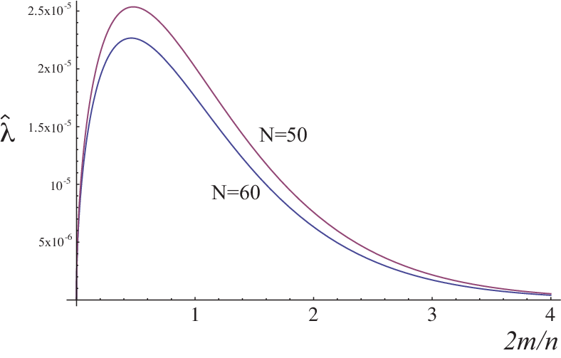
In order for the inflation driven by (23) to last for $N$ e-foldings, the following inequality must be met;

$$\varphi_{N}\;\lesssim\;\kappa^{-n/2}~~\Longleftrightarrow~~~\kappa\;\lesssim\;\left(\frac{n}{4mN}\right)^{\frac{1}{n}}.$$ (27)

For instance, $\kappa$ must be smaller than $0.1$ for for $n=2$, $m=1$ and $N=50$ [6]. The spectral index $n_{s}$ and the tensor-to-scalar ratio $r$ are respectively given by

$$n_{s} = 1-\left(1+\frac{m}{n}\right)\frac{1}{N},$$ (28)

$$r = \frac{8m}{n}\frac{1}{N},$$ (29)

and they are related to each other by

$$1-n_{s}\;=\;\frac{n+m}{8m}r.$$ (30)

The inflation ends when the slow-roll condition is violated at $\varphi\sim 1$, and the inflaton starts to oscillate about the origin. The $\eta$ is no longer stabilized at $\eta_{\rm min}$ for $|\hat{\phi}|<1$. As the amplitude of the inflaton decreases, the symmetry breaking term (9) (or the first term in (16)) becomes more important. For $|\phi|<(\kappa/n^{2})^{1/(2n-2)}$, the Lagrangian becomes

$${\cal L}\;\approx\;\partial^{\mu}\tilde{\phi}^{\dagger}\partial_{\mu}\tilde{\phi}-\frac{\lambda^{2}}{\kappa^{m}}|\tilde{\phi}|^{2m},$$ (31)

where we have defined a canonically normalized field at low scales, $\tilde{\phi}\equiv\sqrt{\kappa}\phi$. The power of the scalar potential changes from $2m/n$ to $2m$ after inflation. The shape of the potential for $m\geq 2$ is shown in Fig. 4. Except for $n=1$, the potential becomes steeper after inflation. (Note that the model with $n=m=1$ is equivalent to the model of Ref. [11].) This is one of the features of the running kinetic inflation. In Ref. [6], the case of $n=2$ and $m=1$ was mainly studied, where the potential is linear during inflation and becomes a quadratic term after inflation.

The inflaton has a large mass at the potential minimum, $m_{\phi}\simeq\lambda/\sqrt{\kappa}$, only if $m=1$. On the other hand, for $m\geq 2$, the inflaton remains massless in the SUSY limit. This opens up a very interesting phenomenon; for instance, if take $n=m\geq 2$, the inflaton is massive during inflation, but it becomes massless after inflation! Thus, the inflaton decay process will be significantly modified compared to the case of the massive inflaton. In the next section we will study the inflaton mass at the potential minimum, taking account of the SUSY breaking effect.

Figure 4: The scalar potential near the origin for $m\geq 2$ with respect to the canonically normalized fields $\tilde{\phi}$ and $\hat{\phi}$. The mass term about the origin represents the soft SUSY breaking mass. We define $\tilde{\phi}_{\rm b}=\kappa^{n/(2n-2)}$ and $\tilde{\phi}_{\rm e}=(m_{3/2}\kappa^{m/2}/\lambda)^{1/(m-1)}$.

II.4 Inflaton mass spectrum

One of the features of the running kinetic inflation model is that the scalar potential becomes steeper some time after inflation. In the SUSY limit, the inflaton mass at the potential minimum depends on the value of $m$. If $m=1$, both inflaton and inflatino have a large SUSY mass, while they are massless for $m\geq 2$. In the latter case, once the SUSY breaking effect is taken into consideration, the inflaton and/or inflatino acquire a soft SUSY breaking mass that depends on $n$. If $n=2$, both the inflaton and inflatino acquire a soft mass heavier than the gravitino mass, while the inflaton mass is of order of the gravitino mass and the inflatino remains massless for $n\geq 3$. We consider these three cases.

II.4.1 A case of $m=1$

Both the inflaton and $X$ have a large and degenerate SUSY mass $\simeq\lambda/\sqrt{\kappa}$, and these two fields are maximally mixed, once a constant term in the superpotential is taken into account [11]. Depending on the precise value of $\kappa$, the mass can vary from $10^{14}{\rm\,GeV}$ up to the Planck mass. Since the inflaton mass is so large that the SUSY breaking effect is negligible.

II.4.2 A case of $n=2$ and $m\geq 2$

In the case of $n=2$ and $m\geq 2$, the inflaton is massless at the potential minimum in the SUSY limit. However, the $\ell=1$ term gives a soft SUSY breaking mass much larger than the gravitino mass.

Let us consider the case of $n=m=2$, and the case of $m\geq 3$ can be treated in the same way. The effective potential around the origin is proportional to $|\tilde{\phi}|^{4}$ (see Eq. (31)). Therefore the inflaton as well as $X$ remain massless in the SUSY limit. In order to estimate their masses we need to take account of the SUSY breaking effect.

To this end, let us introduce a SUSY breaking superfield $Z$, which has a non-zero F-term, $\left\langle F_{Z}\right\rangle\equiv\mu^{2}=\sqrt{3}m_{3/2}$, where $m_{3/2}$ is the gravitino mass. We fix $\left\langle Z\right\rangle=0$, and do not consider its dynamics in the following analysis. The Kähler and super-potentials are

$$K = \kappa|\phi|^{2}+c_{1}(\phi^{2}-\phi^{{\dagger}2})-\frac{1}{2}(\phi^{2}-\phi^{{\dagger}2})^{2}+|X|^{2}+|Z|^{2}+\cdots,$$ (32)

$$W = \lambda X\phi^{2}+\mu^{2}Z+W_{0},$$ (33)

where $W_{0}=m_{3/2}$. In general there could be couplings among $Z$, $\phi$ and $X$ in the Kähler potential, which are denoted by the dots. As long as they are suppressed by the Planck scale, the following result does not change significantly, and so, we drop them in the following.

Let us rewrite the Kähler and super-potentials in terms of $\tilde{\phi}$:

$$K = |\tilde{\phi}|^{2}+\frac{c_{1}}{\kappa}(\tilde{\phi}^{2}-\tilde{\phi}^{{\dagger}2})-\frac{1}{2\kappa^{2}}(\tilde{\phi}^{2}-\tilde{\phi}^{{\dagger}2})^{2}+|X|^{2}+|Z|^{2},$$ (34)

$$W = \frac{\lambda}{\kappa}X\tilde{\phi}^{2}+\mu^{2}Z+W_{0}.$$ (35)

Using the supergravity scalar potential (15), one can show that $\tilde{\phi}$ and $X$ are stabilized at the origin. Their masses at the origin are

$$m_{\tilde{\phi}} = \sqrt{1+\frac{4|c_{1}|^{2}}{\kappa^{2}}}m_{3/2}\;\approx\;\frac{2|c_{1}|}{\kappa}m_{3/2},$$ (36)

$$m_{X} = m_{3/2},$$ (37)

where we have used $\kappa\ll 1$ and $|c_{1}|=O(1)$. As long as the inflaton is coupled to the SUSY breaking field only gravitationally, the inflaton is stabilized at the origin. This is not necessarily the case for $X$; the origin could be destabilized depending on a possible quartic coupling $|X|^{2}|Z|^{2}$ in the Kähler potential. Note that $\tilde{\phi}$ and $X$ do not mix in contrast to the case of $n=m=1$. The inflatino has the same mass as the inflaton.

The result changes if we impose the $Z_{2n}$ discrete symmetry. In this case $c_{1}$ should vanish, and the inflaton mass becomes of order of the gravitino mass.

II.4.3 A case of $n\geq 3$ and $m\geq 2$

Similarly we consider the case of $n=m=3$; the other cases can be treated along the same line. In the case of $n=m=3$, the inflaton and $X$ are massless in the SUSY limit as in the previous case. Let us write down the Kähler and super-potentials (13) and (14) in terms of $\tilde{\phi}$:

$$K = |\tilde{\phi}|^{2}+\frac{c_{1}}{\kappa^{3/2}}(\tilde{\phi}^{3}-\tilde{\phi}^{{\dagger}3})-\frac{1}{2\kappa^{3}}(\tilde{\phi}^{3}-\tilde{\phi}^{{\dagger}3})^{2}+|X|^{2}+|Z|^{2},$$ (38)

$$W = \frac{\lambda}{\kappa^{3/2}}X\tilde{\phi}^{3}+\mu^{2}Z+W_{0}.$$ (39)

Using the supergravity scalar potential (15), one can show that $\tilde{\phi}$ and $X$ are stabilized at the origin. Their masses at the origin are

$$m_{\tilde{\phi}} = m_{X}=m_{3/2}.$$ (40)

For a general Kähler potential, both the inflaton and $X$ have a mass of $O(m_{3/2})$. The inflatino still remains massless. As we will see later, if we couple the inflaton to the Higgs sector, the inflatino acquires a mass after the electroweak phase transition.

II.5 Solution to the non-thermal gravitino production

In order to have a successful inflation model, one needs to recover the hot radiation-dominated Universe after inflation. This is achieved by the inflaton decay, which transfers the inflaton energy to radiation. Recently it was pointed out that a significant amount of gravitinos can be produced by the inflaton decay [11]; the resultant gravitino abundance is given by an increasing function of the inflaton mass and VEV at the potential minimum, giving a preference to a light mass and a small VEV.

Our running kinetic inflation model is a variant of the chaotic inflation, and so, it belongs to a high-scale inflation. Interestingly, our model avoids the gravitino overproduction problem in two ways. First, the inflaton has a discrete symmetry, which forbids the inflaton VEV. Even if the symmetry is explicitly broken by a small amount, the induced VEV could be suppressed. Secondly, the inflaton is very light at the minimum for $m\geq 2$, and indeed, it is massless in the SUSY limit. As we have seen before, the inflaton mass is of order of the gravitino mass in most cases, which can suppress the inflaton decay into the gravitinos. Such a kinematic suppression of the gravitino production is a new and attractive solution to the non-thermal gravitino production. What is particularly nice about our model is that the inflaton potential during inflation is different from that at the minimum, and the inflation model can be well within the WMAP allowed region, without invoking a non-minimal coupling to the gravity.

II.6 Reheating

II.6.1 A case of $m=1$

In order to reheat the Universe, the inflaton must have some couplings with the SM sector. In the case of $m=1$, the inflaton mass is heavier than $10^{14}{\rm\,GeV}$, and the inflaton and $X$ are maximally mixed in general [11]. Therefore $\phi$ can decay into the SM particles through couplings of $X$ with the SM sector. For instance, if we introduce the coupling with Higgs doublets [28],

$$W\;=\;\lambda_{X}XH_{u}H_{d},$$ (41)

where $\lambda_{X}$ is a numerical coefficient and $H_{u(d)}$ is the up(down)-type Higgs doublet, the reheating temperature will become

$$T_{R}\;\sim\;10^{10}{\rm\,GeV}\left(\frac{\lambda_{X}}{10^{-5}}\right)\left(\frac{m_{\phi}}{10^{14}{\rm\,GeV}}\right)^{1/2}.$$ (42)

Here we have assumed that $H_{u}H_{d}$ has a $R$-charge $0$ and a negative parity under the $Z_{2}$ symmetry. Alternatively, if we allow a symmetry-breaking term $\delta(\phi+\phi^{\dagger})=\delta/\sqrt{\kappa}(\hat{\phi}+\hat{\phi}^{\dagger})$ in the Kähler potential, the inflaton decays into the SM particles through the gravitational couplings with the top Yukawa interaction and the SU(3)_C gauge sector [29, 12]. The reheating temperature will become

$$T_{R}\;\sim\;5\times 10^{6}{\rm\,GeV}\left(\frac{\delta/\sqrt{\kappa}}{10^{-3}}\right)\left(\frac{m_{\phi}}{10^{14}{\rm\,GeV}}\right)^{3/2}.$$ (43)

Note that the $\delta$-term violates both the shift and $Z_{2}$ symmetries. If the inflaton mass $m_{\phi}$ is about $10^{16}{\rm\,GeV}$, the reheating temperature becomes about $10^{10}{\rm\,GeV}$, which is high enough for the thermal leptogenesis to work [30, 31]. However, it is in general difficult to satisfy the constraints from the non-thermal gravitino problem when the inflaton decay is induced by the gravitationally suppressed coupling, unless the gravitino is either extremely light $m_{3/2}\leq O(10)$ eV [32] or very heavy $m_{3/2}\geq O(10^{2})$ TeV and the R-parity is broken. We also note that the inflaton has an approximate U(1) symmetry at the origin, and Q-balls [33] may be formed; however, the charge is relatively small and so it does not affect the reheating process.

II.6.2 A case of $n=2$ and $m\geq 2$

In this case, both the inflaton and $X$ are massless in the SUSY limit. However, once the SUSY breaking is taken into account, the inflaton becomes heavier than the gravitino, while the mass of $X$ is of order of the gravitino mass. In contrast to the previous case, there is no significant mixing between $\phi$ and $X$. So, we need to couple $\phi$ to the SM sector. For instance, we may couple $\phi$ to the Higgs sector,

$$W\;=\;\lambda_{\phi}\phi H_{u}H_{d},$$ (44)

where we have assigned an R-charge $2$ and the $Z_{k}$ charge $-1$ to $H_{u}H_{d}$. The numerical coefficient $\lambda_{\phi}$ breaks the shift symmetry, and so, we may assume $\lambda_{\phi}\sim\lambda$, although not necessarily. Assuming the inflaton mass is much heavier than the Higgs and Higgsinos, the resultant decay temperature would be

$$T_{R}\;\sim\;10^{7}{\rm\,GeV}\,|c_{1}|^{1/2}\left(\frac{\lambda_{\phi}}{10^{-5}}\right)\left(\frac{\kappa}{10^{-4}}\right)^{-\frac{1}{2}}\left(\frac{m_{3/2}}{{\rm TeV}}\right)^{\frac{1}{2}},$$ (45)

where we have used (36). Note that, for the parameters chosen in the above expression, the reheating temperature is comparable to the inflaton mass. If the reheating temperature calculated by equating the decay rate and the Hubble parameter exceeds the inflaton mass, the decay process will be significantly affected by the back reaction. This is because, when the decay products acquire a thermal mass comparable to the inflaton mass, the available phase space will be reduced [34]. That is, the reheating temperature cannot exceed the inflaton mass, as long as it proceeds through a perturbative decay. As a result, the reheating temperature is given by the inflaton mass, if the naively calculated reheating temperature turns out to be larger than the inflaton mass:

$$T_{R}\;\sim\;m_{\phi}=\frac{2|c_{1}|}{\kappa}m_{3/2},$$ (46)

which is used if $T_{R}$ given by Eq. (45) exceeds $m_{\phi}$. The validity of (46) will be discussed in the next section.

II.6.3 A case of $n\geq 3$ and $m\geq 2$

The main difference from the previous case is that the inflaton mass is of order of the gravitino mass, and the reheating temperature becomes lower, accordingly. In particular, in order to reheat the Universe with such a light inflaton mass, the inflaton must have unsuppressed couplings to the SM sector. If it has only gravitationally suppressed interactions, there would be cosmological difficulties; the reheating temperature is too low to be consistent with BBN, and the LSPs may be overproduced by the inflaton decay [35], as long as we consider $m_{3/2}\lesssim O(100)$TeV. Thus, we consider a possibility to couple the inflaton to the SM particles at the renormalizable level. The only possibility is to couple $\phi$ to the Higgs sector as in Eq. (44). If we calculate the reheating temperature by equating the decay rate to the Hubble parameter, we would obtain a temperature much higher than the inflaton mass. Thus, according to the above argument, the reheating temperature is equal to the inflaton mass:

$$T_{R}\;\sim m_{\phi}\sim m_{3/2}.$$ (47)

As a corollary, the inflaton mass, therefore the gravitino mass, needs to be heavier than $O(10)$ MeV to be consistent with BBN [36, 37, 38], since otherwise the reheating would not be completed before BBN.

Let us discuss the validity of the reheating temperature, $T_{R}\sim m_{\phi}$. So far we have not taken into account that, before the inflaton decay is completed, the decay products, $H_{u}$ and $H_{d}$, have masses of $O(\lambda_{\phi}|\phi|)$, which may prevent the inflaton decay to proceed until the amplitude becomes small enough. As we will see later, the inflaton moves in a nearly circular orbit in the complex plane, and so, the mass of the decay products does not change during oscillations. The decay into Higgs (Higgsino) becomes first kinematically accessible when the amplitude of oscillations becomes $\tilde{\phi}\sim\sqrt{\kappa}m_{3/2}/\lambda_{\phi}$. If the inflaton decayed at this epoch, the reheating temperature would be $T_{R}\sim\kappa^{1/4}\lambda_{\phi}^{-1/2}m_{3/2}$. If the temperature estimated this way exceeds the inflaton mass, the decay cannot complete the reheating due to the back reaction of the thermal mass, and the actual reheating temperature is given by $T_{R}\sim m_{\phi}$. This is indeed the case if $\kappa\gtrsim\lambda_{\phi}^{2}$. Otherwise, the reheating temperature is given by $T_{R}\sim\kappa^{1/4}\lambda_{\phi}^{-1/2}m_{3/2}$, but this does not modify our argument qualitatively, because the $\kappa$ is expected to be not much smaller than $O(\lambda_{\phi}^{2})$ (see the discussion below Eq. (9)).

In the above analysis we implicitly assumed that the inflaton is oscillating about the origin with an amplitude smaller than $\tilde{\phi}_{\rm e}=(m_{3/2}\kappa^{m/2}/\lambda)^{1/(m-1)}$ so that the inflaton mass is simply given by $O(m_{3/2})$. However, the inflaton decay may proceed before the kination epoch ends, namely, when the amplitude is larger than $\tilde{\phi}_{\rm e}$. In particular, the inflaton has a larger mass (i.e. the energy per unit inflaton quanta) in this regime, and so, it might be possible for the inflaton to transfer a significant amount of energy to radiation. The effective mass for the inflaton during the kination regime is given by $m_{\phi}(\tilde{\phi})\sim\lambda{\tilde{\phi}}^{m-1}/\kappa^{m/2}$, which decreases faster than the effective mass of $H_{u}$ and $H_{d}$. Thus, if $m_{\phi}(\tilde{\phi}_{\rm b})<\lambda_{\phi}\tilde{\phi}_{\rm b}/\sqrt{\kappa}$, the inflaton decay does not occur during the kination epoch, where $\tilde{\phi}_{\rm b}=\kappa^{n/(2n-2)}$ is the inflaton field value at the beginning of kination. This condition is rewritten as $\kappa^{(m-n-1)/(2n-2)}\lambda<\lambda_{\phi}$. If this condition is not met, we need to take account of the radiation generated during the kination epoch. The radiation could dominate the energy density of the Universe, and the inflaton may be subdominant at the decay, or it may dominate the Universe again.

Furthermore, the actual situation could be more complicated, because the inflaton also decays into the gauge bosons and gauginos through the one-loop diagram, even if the tree-level decay is kinematically forbidden. Although the decay rate of such processes is suppressed, a small amount of radiation produced by the process may dominate and terminate the kination regime. Thus, the details of the reheating process and the resulting thermal history of the Universe depend much on the model parameters. In Sec. IV, we fully take into account the tree and one-loop decay processes.

II.7 Preheating

So far we have focused on the perturbative decay, but since the inflaton starts to oscillate from the Planck scale, preheating could be important especially for the early stage of the reheating epoch. How fast and how long it proceeds depends on the interaction with the Higgs field as well as the inflaton trajectory. In particular, it is expected that the inflaton acquires a non-vanishing angular momentum when it starts to oscillate because, the U(1) symmetry of the inflaton potential around the origin is just an accidental one, and at large scales, it is explicitly broken down to $Z_{k}$. If the inflaton acquires large enough angular momentum, it does not pass near the origin, reducing the efficiency of the preheating [39]. In fact we numerically followed the inflaton dynamics and confirmed that the inflaton acquires a large angular momentum at the end of inflation. See Fig. 5. The exception is the case of the $Z_{2n}$ symmetry, in which all $c_{\ell}$ with odd $\ell$ vanish; the inflationary trajectory coincides with the real component of $\phi$, and so, no angular momentum is induced. Therefore, in this case, preheating will play an important role in the reheating. We leave a detailed study of the preheating for future work, and will focus on the case of $Z_{k}$ symmetry with $k\leq n$.

We note that the angular momentum acquired by the inflaton is nothing but a CP asymmetry of the inflaton. Therefore, if the inflaton has a lepton- or baryon-number violating coupling like

$$W\;=\;\lambda^{\prime}\phi LH_{u},$$ (48)

where the $L$ is the lepton doublet, the asymmetry is transformed into the lepton asymmetry. Thus, with the aid of the sphaleron process violating the $B+L$, the baryon asymmetry can be naturally produced by the inflaton decay.

Figure 5: The inflationary trajectory for $n=m$ and $c_{1}=-i$ in the ${\hat{\phi}}=\phi^{2}$ plane. During inflation with $|{\hat{\phi}}|>1$, $Im[\hat{\phi}]$ is stabilized at $1$. After inflation the inflaton acquires a large angular momentum.

III Kination after inflation

III.1 Enhancement of gravity waves

In the present model, the inflaton potential changes its form depending on the field value $\phi$. Correspondingly, the expansion law, or the equation of state, of the Universe changes as well. The transition of the equation of state occurs as follows. After the inflation ends at $|{\hat{\phi}}|\sim 1$, the inflaton oscillates in the potential $V\propto|{\hat{\phi}}|^{2m/n}$ until the amplitude becomes $|{\tilde{\phi}}|\sim\kappa^{1/(2n-2)}$. For the amplitude smaller than $\kappa^{1/(2n-2)}$, the potential behaves as $V\propto|{\tilde{\phi}}|^{2m}$: this is the kination regime. As the amplitude further decreases, the potential becomes finally dominated by the soft mass term $\propto|{\tilde{\phi}}|^{2}$, which corresponds to the matter-dominated Universe. Then the inflaton decays and the radiation dominant Universe begins. The evolution of the Universe described above leaves a characteristic imprint on the spectrum of inflationary gravitational wave background [40, 41, 42, 43]. In particular, the kination after inflation enhances the gravity waves at corresponding frequencies, and the direct detection of gravitational waves by spaceborne laser interferometers may support or refute the expansion history of the Universe.

In the following analysis we simply assume that the background plasma, which may already exist in the kination regime, does not affect the expansion history. Let us denote the Hubble parameter at the beginning and the end of kination as $H_{\rm b}$ and $H_{\rm e}$, respectively. They are estimated as $H_{\rm b}\sim\lambda\kappa^{m/(2n-2)}$ and $H_{\rm e}\sim(\kappa^{m/2}m_{3/2}^{m}/\lambda)^{1/(m-1)}$. If the kination regime is followed by the matter-dominated regime, the reheating temperature is given by $T_{R}\sim m_{3/2}$, as explained before. As an extreme case, we also consider a case that inflaton decays as soon as the kination ends, and the reheating temperature is then given by $T_{R}\sim\sqrt{H_{\rm e}}$, although some non-trivial process may be needed to realize this situation. During the kination stage, the scale factor grows as $a(t)\propto t^{(m+1)/(3m)}$. The spectrum of the gravitational waves which enters the horizon at this stage looks like $\Omega_{\rm GW}(k)\propto k^{(2m-4)/(2m-1)}$ with a comoving wave number $k$. Here we have defined

$$\Omega_{\rm GW}(k)=\frac{1}{\rho_{0}}\frac{d\rho_{\rm GW}(k)}{d\ln k},$$ (49)

where $\rho_{0}$ is the critical density of the Universe, and $d\rho_{\rm GW}(k)/d\ln k$ denotes the energy density of the gravitational waves per logarithmic frequency.

Therefore, the gravitational wave spectrum behaves as

$$\Omega_{\rm GW}(k)\propto\left\{\begin{array}[]{ll}k^{0}&{\rm for}~~k_{\rm eq}<k<k_{\rm R},\\ k^{-2}&{\rm for}~~k_{\rm R}<k<k_{\rm e},\\ k^{(2m-4)/(2m-1)}&{\rm for}~~k_{\rm e}<k<k_{\rm b},\end{array}\right.$$ (50)

if $k_{\rm R}<k_{\rm e}$, where $k_{\rm eq},k_{\rm R},k_{\rm e}$ and $k_{\rm b}$ denote the comoving horizon scale at the time of matter-radiation equality, reheating, the end of kination and the beginning of kination. We find $k_{\rm R}=2.6\times 10^{-5}~{\rm Hz}(T_{\rm R}/1{\rm TeV})(g_{*s}(T_{\rm R})/106.75)^{1/6}$, $k_{\rm e}=(H_{\rm e}/H_{\rm R})^{1/3}k_{\rm R}$ and $k_{\rm b}=(H_{\rm b}/H_{\rm e})^{(2m-1)/(3m)}k_{\rm e}$. Importantly, the spectrum is enhanced in the kination regime for $m>2$.

In the extreme case that the reheating occurs as soon as the kination ends, we can set $k_{\rm R}=k_{\rm e}$ in Eq. (50):

$$\Omega_{\rm GW}(k)\propto\left\{\begin{array}[]{ll}k^{0}&{\rm for}~~k_{\rm eq}<k<k_{\rm R},\\ k^{(2m-4)/(2m-1)}&{\rm for}~~k_{\rm R}<k<k_{\rm b},\end{array}\right.$$ (51)

Thus the gravitational wave spectrum has no suppression in this case.

Fig. 6 shows the spectrum of gravitational waves for $n=4$ and $m=3$, for the case of (a) reheating immediately after kination ends, (b) $\kappa=\lambda^{2}$ and (c) and $\kappa=\lambda$. The projected sensitivities of BBO/DECIGO [44, 45] its correlation analysis, and its ultimate sensitivities are also shown. We can clearly see the enhancement at high frequency corresponding to the mode entering in the horizon during the kination regime where the potential is given by $V\propto|{\tilde{\phi}}|^{6}$. However, this enhancement is compensated to some extent by the suppression due to the subsequent matter-dominated era. Which effect dominates depends on the parameter $\kappa$ and $\lambda$.

In most cases, the spectrum has characteristic features on its magnitude and/or the tilt at observable frequencies. If the primordial gravitational waves is discovered by the future CMB observations, we may have a good chance to detect them directly by the planned space laser interferometers and to confirm the running kinetic inflation model.

Figure 6: Spectrum of gravitational wave background for $n=4$ and $m=3$, for the case of (a) reheating immediately after kination ends, (b) $\kappa=\lambda^{2}$ and (c) and $\kappa=\lambda$. The projected sensitivities of BBO/DECIGO and its correlation analysis are also shown.

III.2 Enhancement of unwanted relics : gravitino

The modified expansion history of the Universe enhances not only primordial gravitational waves, but also the abundance of unwanted relics. The gravitino is one of such dangerous relics. Let us estimate its abundance.

At the inflationary stage, the Universe is regarded as being filled with radiation with Hawking temperature $\sim H_{I}/(2\pi)$. Thus particles with masses smaller than $H_{I}$ would have thermal abundances [46]. The gravitino number density at the end of inflation is given by $n_{3/2}(H_{I})\simeq\gamma H_{I}^{3}$, where $\gamma\simeq 7\times 10^{-4}$. The number density after the reheating completes is estimated as

$$\begin{split}n_{3/2}(H_{R})&=n_{3/2}(H_{I})\left(\frac{a(H_{I})}{a(H_{\rm b})}\right)^{3}\left(\frac{a(H_{\rm b})}{a(H_{\rm e})}\right)^{3}\left(\frac{a(H_{\rm e})}{a(H_{\rm R})}\right)^{3}\\ &\sim\gamma H_{I}^{3}\left(\frac{H_{\rm b}}{H_{I}}\right)^{(m+n)/m}\left(\frac{H_{\rm e}}{H_{\rm b}}\right)^{(m+1)/m}\left(\frac{H_{\rm R}}{H_{\rm e}}\right)^{2}.\end{split}$$ (52)

Thus the gravitino abundance in terms of the number-to-entropy ratio is given by

$$Y_{3/2}\equiv\frac{n_{3/2}}{s}\sim\frac{\gamma\lambda}{4}\frac{H_{I}}{M_{P}}\left(\frac{H_{I}}{\lambda M_{P}}\right)^{(m-n)/m}.$$ (53)

This is evaluated as

$$Y_{3/2}\sim 7\times 10^{-14}\left(\frac{\lambda}{10^{-5}}\right)\left(\frac{H_{I}}{10^{14}{\rm GeV}}\right)\left(\frac{H_{I}}{\lambda M_{P}}\right)^{(m-n)/m}.$$ (54)

Here we have taken $T_{R}=m_{3/2}$. The constraint reads $m_{3/2}Y_{3/2}\lesssim 4\times 10^{-10}$GeV for a stable gravitino and $Y_{3/2}\lesssim 10^{-16}$ for $m_{3/2}\sim 1$ TeV and $Y_{3/2}\lesssim 10^{-13}$-$10^{-12}$ for $m_{3/2}\sim 10$-$100$ TeV for an unstable gravitino [47]. Therefore, even if the gravity waves are enhanced by the kination epoch, the gravitationally produced gravitino is cosmologically harmless for a light stable gravitino ($m_{3/2}\lesssim 100$GeV) or a heavy gravitino ($m_{3/2}\gtrsim 10$TeV). In the next section, we consider a case that the inflaton is identified with a singlet field in the nMSSM, where it turns out that there is no such enhancement, and therefore no cosmological problem with the gravitationally produced gravitino.

IV Inflaton embedded in nMSSM

The inflaton and inflatino remain massless in the SUSY limit for $m\geq 2$, as we have seen in Sec. II. If $n\geq 3$, once the SUSY breaking is taken into account, the inflaton acquires a mass of $O(m_{3/2})$, while the inflatino acquires its mass through a coupling to the Higgs sector, (44). Since the inflaton and inflatino are light, they may play an important role in the low energy.

The MSSM plus a singlet that couples to the Higgs sector as (44) is known as nMSSM. The main motivation to promote the $\mu$-parameter to the singlet superfield is to solve the $\mu$-problem. In order for the singlet to develop a VEV of the order of the electroweak scale, a $Z_{5}$ or $Z_{7}$ R-symmetry is imposed on the theory; the tadpole for the singlet is then radiatively induced at sufficiently high order with a desired magnitude. The difference from the so called Next to Minimal SUSY SM (NMSSM) is the absence of both the cubic self-coupling of the singlet and the domain wall problem associated with the spontaneously broken $Z_{3}$ symmetry. The discrete R-symmetry adopted in nMSSM forbids the cubic self-coupling, and get rid of the domain wall problem from the theory without destabilizing the hierarchy. The nMSSM has rich phenomenology; the singlino is a viable candidate for dark matter, and the electroweak baryogenesis is feasible [48]. We here show that the running kinetic inflation model can nicely fit with the nMSSM, with the additional singlet being identified with the inflaton.

We have assigned non-zero discrete charges to $H_{u}H_{d}$ in Eq. (44), and so, we may wonder if domain walls are produced at the electroweak phase transition. This can be solved if we consider a discrete R-symmetry, which is explicitly broken by the constant term $W_{0}$ in the superpotential. So far we have imposed two symmetries, the R-symmetry and the discrete $Z_{k}$ symmetry on the inflaton and $X$. We can combine these two and consider a discrete $Z_{kR}$ symmetry, with $k$ being a divisor of $2n$. Under the $Z_{kR}$ symmetry, $(\phi^{n}-\phi^{{\dagger}n})$ is invariant (up to a phase factor for $k=2n$). The charge assignment is given by Table 2. Note here that the superpotential has a R-charge $6$ in this charge assignment.

In order to have a successful inflation, there are several operators that must be suppressed. In particular, we require that $W\supset X,X^{2}$ and $X^{2}\phi^{m}$ should be forbidden by the discrete R symmetry, because these operators cannot be simply set to zero by the shift symmetry. We note that, although the discrete R symmetry on $\phi$ is chosen so that it is consistent with the shift symmetry (6), the operators including $\phi$ in the superpotential allowed by the discrete R symmetry do break the shift symmetry. Therefore we cannot estimate naively the magnitudes of those operators. In this sense, it is minimal to require that those three operators should be forbidden by the discrete R symmetry. We simply assume that the other type of dangerous operators are sufficiently suppressed by the shift symmetry. This restricts the possible values of $m$: only $m=1,3,6$ and $8$ are allowed for $m\leq 10$. (In the case of the $Z_{7}$ R symmetry, the allowed values of $m(\leq 14)$ are $m=1,2,3,4,8,9,10$ and $11$.)

In order to account for the correct abundance of the inflatino dark matter, the effective coupling $\lambda_{\phi}/\sqrt{\kappa}$ must be of order unity. This is indeed the case if $\kappa$ is radiatively generated by the interaction (44). Furthermore, the inflatino must be long-lived to account for the dark matter. This is the case if the inflatino is the LSP and the R-parity is conserved. We note however that the fermionic superpartner of $X$ could be the LSP, partially because we have forbidden its mass term $W\supset X^{2}$ by the discrete R symmetry. Even in this case, the inflatino would be sufficiently long-lived against the decay into $\tilde{X}$, if $m\geq 4$. Also, if $m=2$ and $\lambda/\kappa\approx\lambda_{\phi}/\sqrt{\kappa}$, the inflatino mass can become comparable to the ${\tilde{X}}$.

	$H_{u}$, $H_{d}$	$Q$, $L$	$U^{c}$, $D^{c}$, $E^{c}$	$\phi$	$X$	$W$
$Z_{5R}$, $Z_{7R}$	$1$	$2$	$3$	$4$	$6-4m$	$6$

Table 2: The charge assignment of the $Z_{5R}$ and $Z_{7R}$ symmetries. Note that the charge of the superpotential is normalized to be $6$.

We have estimated the spectrum of primordial gravitational waves in the setup embedded in the nMSSM, as shown in Fig. 7; $n=5$ and $m=3$ with $\kappa=10^{-5}$ and $10^{-4}$ (left panel), and $n=7$ and $m=4$ with $\kappa=10^{-6}$ and $10^{-5}$ (right panel). As explained in Sec. II, the actual thermal history is complicated due to the existence of the background plasma produced by the loop-suppressed inflaton decay. In this plot we have fully taken into account the effect of decay products by the tree and one-loop inflaton decay processes on the expansion history. The spectrum becomes flat for $\kappa=10^{-6}$ in the right panel of Fig. 7, because the radiation produced during the kination comes to dominate the Universe for some time.

Figure 7: Spectrum of gravitational wave background for the case of $n=5$ and $m=3$ with $\kappa=10^{-5}$ and $10^{-4}$ (left panel), and $n=7$ and $m=4$ with $\kappa=10^{-6}$ and $10^{-5}$ (right panel), which are embedded in the nMSSM framework. The projected sensitivities of BBO/DECIGO and its correlation analysis are also shown.

V Conclusions

In this paper we have studied the running kinetic inflation model, motivated by a simple idea that the kinetic term may well change its form if the inflaton moves over more than the Planck scale. The growth of the kinetic term is actually advantageous for the inflation to occur, because the effective potential for the canonically normalized field becomes flat. As a conrete example, we have constructed a variety of chaotic inflation models in supergravity. One of the features of the running kinetic inflation is that the power of the potential increases after inflation: the potential is given by $\phi^{2m/n}$ during inflation, while it becomes $\phi^{2m}$ after inflation. The scalar spectral index and the tensor-to-scalar ratio are given by $n_{s}=1-\left(1+\frac{m}{n}\right)\frac{1}{N}$ and $r=\frac{8m}{n}\frac{1}{N}$, respectively. Interestingly, the tensor-to-scalar ratio is generically large enough to be discovered by the CMB observation in future, especially by the Planck satellite.

We have found that the model has a lot of interesting implications. In particular, we have focused on the case of $m\geq 2$, in which the inflaton is massless at the potential minimum in the SUSY limit. Once the SUSY breaking effect is taken into account, the inflaton acquires a mass of the order of the gravitino mass, in general. Because of such a light mass, the thermal and non-thermal gravitino production can be naturally avoided. Also we have seen that the gravity waves can be enhanced due to the kination epoch which is naturally present in the running kinetic inflation. Finally, we have pointed out that, in order to have a successful reheating with such a light inflaton mass, the inflaton needs to have unsuppressed couplings with the SM sector. One plausible candidate is the coupling to the Higgs sector (44). Then the model is similar to the so called nMSSM with the singlet identified with the inflaton. The discrete R symmetry introduced in nMSSM can be identified with the discrete symmetry on the inflaton, and therefore the running kinetic inflation naturally fits with nMSSM. The phenomenology of nMSSM is known to be rich; the inflatino can account for the dark matter, and the inflaton coupling enables the electroweak baryogenesis.

The running inflation model, if realized in nature, will be confirmed in coming years by the CMB observations. Interestingly, if $m\geq 2$, the inflaton and/or inflatino may be discovered at the collider experiments such as LHC as well as the direct DM search.