Elliptic flow: pseudorapidity and number of participants dependence

Abstract

We discuss the elliptic flow dependence on pseudorapidity and number of participating nucleons in the framework of string percolation, and argue that the geometry of the initial overlap region of interaction, projected in the impact parameter plane, determines the experimentally measured azimuthal asymmetries. We found good agreement with data.

The discovery of the large elliptic flow $v_{2}$ was one of the most important achievements at RHIC experiments [1-9]. A non vanishing anisotropic flow exist only if the particles measured in the final state depend not only on the local physical conditions realized at the production but as well on the global event geometry. In a relativistic local theory, this non local information can only emerge as a collective effect, requiring interactions between the relevant degrees of freedom, localized at different points of the collision region. In this sense, anisotropic flow is particularly unambiguous and convincing manifestation of collective dynamics in heavy ion collisions [10].

The elliptic flow $v_{2}$ can be qualitatively explained as follows. In a collision at high energy the spectators are fastly moving opening the way, leaving behind at mid- rapidity an almond shaped azimuthally asymmetric region of QCD matter. This spatial asymmetry implies unequal pressure gradients in the transverse plane, with a larger density gradient in the reaction plane ( in- plane). As a consequence of subsequent multiple interactions between degrees of freedom this spatial asymmetry leads to an anisotropy in momentum plane. The final particle transverse momentum is more likely to be in- plane than in the out- plane, with $v_{2}>0$ as predicted [11].

The basic idea of our model [12] is that the angular azimuthal anisotropy associated to the geometry of the first stages in the collision - the projected almond- influences in a determinant way the presence or not of the flow. In other words if the projected overlap region was a circle we would have $v_{2}\equiv 0$. As in the almond case the small axis is in the reaction plane, corresponding to higher matter density, then $v_{2}>0$.

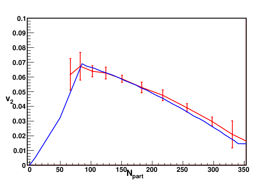
Our model was introduced in [12] and a discussion of applications and conjectures were presented dependence of $v_{2}$ on the produced hadron, validity of quark counting rules, applications to nuclear reduction factors, etc. Here we just want to call attention to $v_{2}$ as a function of pseudorapidity $\eta$ and the number of participants $N_{A}$ for nucleus A, after the integration over $p_{T}^{2}$. The triangle shape shown by the data on the dependence of $v_{2}$ on $\eta$ it is not easy reproduced by models as it has been recently emphasized [13]. We show that string percolation model is able to do it.

The string percolation model [14] develops around the concept of transverse density $\eta^{t}$,

$$\eta^{t}=(\frac{r_{0}}{R})^{2}\bar{N}^{s}$$ (1)

, where $\bar{N}^{s}$ is the number of longitudinal strings formed in the collision, $r_{0}$ is the radius of the single string and $R$ the effective radius of the interaction overlap region $S$ in the impact parameter b,

$$S=\pi R^{2}$$ (2)

with

$$S=2R_{A}^{2}[cos^{-1}(\beta)-\beta\sqrt{1-\beta^{2}}]$$ (3)

, $R_{A}$ being the nuclear radius and

$$\beta=\frac{b}{2R_{A}}$$ (4)

Two relations, one for the particle density $dn/d\eta$ and the other for the average transverse momentum squared define the essential features of the model [13,14]

$$dn/d\eta=F(\eta^{t})\bar{N}^{s}\mu_{1}$$ (5)

and

$$<p_{T}^{2}>=<p_{T}^{2}>_{1}/F(\eta^{t})$$ (6)

where $\mu_{1}$ and $<p_{T}^{2}>_{1}$ are single string parameters and $F(\eta^{t})$ is the colour reduction factor [15]:

$$F(\eta^{t})=\sqrt{\frac{1-e^{-\eta^{t}}}{\eta^{t}}}.$$ (7)

We introduce now two reasonable approximations: that $N^{s}$ is proportional to the number of binary collisions and that $R$ is proportional to the proton radius,

$$\bar{N}^{s}\sim\bar{N}^{s}_{p}N_{A}^{4/3}$$ (8)

and

$$R=R_{p}N_{A}^{1/3},$$ (9)

where $N_{p}^{s}$ and $R_{p}$ are proton parameters and $N_{A}$ is the number of participants from nucleus A.

From (1), (8) and (9) we obtain

$$\eta^{t}_{N_{A}}=\eta^{t}_{p}N_{A}^{2/3}.$$ (10)

By using (9) and (1) on (5) one obtains

$$\frac{1}{N_{A}^{2/3}}\frac{dn}{d\eta}=F(\eta^{t})\eta^{t}(\frac{R_{p}}{r_{0}})^{2}\mu_{1}$$ (11)

, and we observe that the right hand side of (11) and (6) are deeply related.

This kind of results appears in the Color Glass Condensate (CGC) [16] and in string percolation [14,17]. Note that (11) can be written in the form

$$\sqrt{(1-\exp{-\eta^{t}})\eta^{t}}=\frac{\pi r_{0}^{2}}{\mu_{1}}[\frac{1}{S}\frac{dn}{d\eta}]$$ (12)

This relation, as we shall see, is essential to understand the (pseudo)rapidity and number of participants per nucleus dependence of $v_{2}$: $v_{2}(\eta,N_{A})$. Note that in (12) small $\eta^{t}$ corresponds to large $\eta$ and large $\eta^{t}$ to small $\eta$.

Regarding $p_{T}^{2}$ distributions, we started with Schwinger gaussian formula, including fusion and percolation (via $F(\eta^{t})$) and clustering fluctuations (via the parameter $k(\eta^{t})$) to obtain[18]:

$$\frac{d^{2}n}{dp_{T}^{2}d\eta}=\frac{dn}{d\eta}\frac{k-1}{k}\frac{F(\eta^{t})}{<p_{T}^{2}>_{1}}\frac{1}{(1+\frac{F(\eta^{t})p_{T}^{2}}{k<p_{T}^{2}>_{1}})^{k}}.$$ (13)

Most of the RHIC data are well described by formula (13) [12,18,19].

In order to discuss directional production along the azimuthal angle $\varphi$, we shall introduce a convenient variable

$$X=F(\eta^{t})p_{T}^{2},$$ (14)

and $X_{\varphi}$

$$X_{\varphi}=F(\eta_{\varphi}^{t})p_{T}^{2},$$ (15)

with

$$\eta_{\varphi}^{t}=\eta^{t}(\frac{R}{R_{\varphi}})^{2}$$ (16)

such that we can simplify notation

$$\frac{dn}{dp_{T}^{2}dy}\rightarrow f(X)$$ (17)

$$\frac{dn}{dp_{T}^{2}dyd\varphi}\rightarrow f(X_{\varphi})$$ (18)

Expanding now $X_{\varphi}$ or $R_{\varphi}$ around $X$ or $R^{2}$ we write

$$f(X_{\varphi})\simeq\frac{2}{\pi}f(X)[\frac{1+\partial lnf(X)}{\partial R}(R^{2}_{\varphi}-R^{2})]$$ (19)

Note that (12) satisfies the normalization condition

$$\int_{0}^{\pi/2}f(X_{\varphi})d\varphi=f(X)$$ (20)

because $R^{2}=<R_{\varphi}^{2}>[12]$. Finally we obtain for $v_{2}$, a function of several variables including $p_{T}^{2}$, $\eta$ and $N_{A}$,

$$v_{2}=\frac{2}{\pi}\int_{0}^{\pi/2}d\varphi cos(2\varphi)(\frac{R_{\varphi}}{R}^{2})\frac{1}{2}\frac{e^{-\eta^{t}}-F(\eta^{t})^{2}}{F(\eta^{t})^{2}}\frac{F(\eta^{t})p_{T}^{2}/<p_{T}^{2}>_{1}}{1+F(\eta^{t})^{2}p_{T}^{2}/k<p_{T}^{2}>_{1}}$$ (21)

which we shall write as the product of tree factors,

$$v_{2}=[\varphi][\eta^{t}][F(\eta^{t})p_{T}^{2}],$$ (22)

$$[\varphi]=\frac{2}{\pi}\int_{0}^{\pi/2}d\varphi cos(2\varphi)(\frac{R_{\varphi}}{R}^{2}),$$ (23)

or, having present that

$$\frac{R_{\varphi}}{R_{A}}=\frac{\sin{\varphi-\alpha}}{\sin{\varphi}}$$ (24)

and

$$\alpha=sin^{-1}(\beta sin\varphi),$$ (25)

$$[\varphi]=\frac{2}{\pi}\int_{0}^{\pi/2}d\varphi\frac{cos(2\varphi)sin^{2}(\varphi-\alpha)}{sin^{2}\varphi}(\frac{R_{A}}{R})^{2},$$ (26)

$$[\eta^{t}]=\frac{1}{2}\frac{e^{\eta^{t}}-F(\eta^{t})^{2}}{F(\eta^{t})^{2}}$$ (27)

and

$$[F(\eta^{t})p_{T}^{2}]=\frac{F(\eta^{t})p_{T}^{2}/<p_{T}^{2}>_{1}}{1+\frac{F(\eta^{t})p_{T}^{2}}{k<p_{T}^{2}>_{1}}}.$$ (28)

Let us next look at the factor $[\varphi]$, (23) in (21) and consider, for fixed $\eta$ and $\sqrt{s}$, two limits:

$i)$ $b\rightarrow 0$ or $\beta\rightarrow 0$ or $N_{A}\rightarrow A$ which implies, (25), $\alpha\rightarrow 0$. We then have $[\varphi]\rightarrow 0$, $[\eta^{t}]$, (27),$\rightarrow$ constant, and $[F(\eta^{t})p_{T}^{2}]\rightarrow 0$, or:

$$N_{A}\rightarrow A\mbox{ , }v_{2}(p_{T}^{2})\rightarrow 0$$ (29)

.

$ii)$ $b\rightarrow 2R_{A}$ or $\beta\rightarrow 1$ or $N_{A}\rightarrow 0$ which implies, (18), $\alpha\rightarrow\varphi$. We then have $[\varphi]\rightarrow 0$, $[\eta^{t}]\rightarrow$ constant, $[F(\eta^{t})p_{T}^{2}]\rightarrow$ some finite function of $p_{T}^{2}$, or:

$$N_{A}\rightarrow 0\mbox{ , }v_{2}(p_{T}^{2})\rightarrow 0$$ (30)

If we look now to the $p_{T}^{2}$ dependence of $v_{2}$ in $[F(\eta^{t})p_{T}^{2}]$, (28) we see that $v_{2}\rightarrow 0$ as $p_{T}^{2}\rightarrow 0$ and $v_{2}\rightarrow k\sim$ constant, as $p_{T}^{2}\rightarrow\infty$. This is observed in data [20].

We perform next the integration in $p_{T}^{2}$, weighted by $\frac{dn}{dp_{T}^{2}d\eta}/\frac{dn}{d\eta}$, to obtain:

$$v_{2}=\frac{2}{\pi}\int_{0}^{\pi/2}d\varphi cos(2\varphi)(\frac{R_{\varphi}}{R})^{2}\frac{e^{-\eta^{t}}-F(\eta^{t})^{2}}{2F(\eta^{t})^{3}}\frac{R}{R-1}=[\varphi][\eta^{t}]^{\prime}$$ (31)

, $[\eta^{t}]^{\prime}$ being different from $[\eta^{t}]$ and $\eta^{t}$ being related to $\eta$ by relation (12). Applying now to $v_{2}(\eta)$ the arguments used for $v_{2}(p_{T}^{2})$ we have:

$$i)N_{A}\rightarrow A\mbox{, }v_{2}(\eta)\rightarrow 0,$$ (32)

with $[\eta^{t}]^{\prime}$ being some negative number depending on $\eta$;

$$ii)N_{A}\rightarrow 0\mbox{, }v_{2}(\eta)\rightarrow 0,$$ (33)

with $[\eta^{t}]^{\prime}\rightarrow 0$.

In conclusion, both $v_{2}(p_{T}^{2})$ and $v_{2}(\eta)$ go to zero as $N_{A}\rightarrow A$ and $N_{A}\rightarrow 0$. In the case of $v_{2}(p_{T}^{2})$ with $p_{T}^{2}\equiv 0$, $v_{2}(p_{T}^{2})$ is identically zero.

As $[\eta^{t}]$ is, in modulus, a growing function of $\eta^{t}$, it is clear that $v_{2}(\eta)$, at fixed $\eta$, is a growing function of energy and of $N_{A}$ see [20].

Regarding $v_{2}$ normalized by the eccentricity $\epsilon$,

$$v_{2}(\eta)/\epsilon,$$ (34)

, with

$$\epsilon=\frac{\sqrt{1+\beta}-\sqrt{1-\beta}}{\sqrt{1+\beta}}$$ (35)

having the limits

$$\beta\rightarrow 0\mbox{, }\epsilon\rightarrow\beta\rightarrow 0$$ (36)

and

$$\beta\rightarrow 1\mbox{ , }\epsilon\rightarrow 1$$ (37)

We see that

$i)$ $N_{A}\rightarrow A$, $R\rightarrow 0$, $v_{2}(\eta)/\epsilon\rightarrow$ constant, increasing with $\sqrt{s}$ and $N_{A}$

$ii)$ $N_{A}\rightarrow 0$, $\beta\rightarrow 1$, $v_{2}(\eta)/\epsilon\rightarrow 0$.

In order to compare with experimental data the dependence of $v_{2}$ on the pseudorapidity, we start with the $\frac{dn}{d\eta}$ data of PHOBOS collaboration [20] taken at $N_{part}=211$. From formula (12) we compute $\eta^{t}$ at each value of $\eta$ and then $v_{2}$ using equation (31). Our result together with the experimental data [20] is presented in fig 1. In the same way, using equation (31) we compute the dependence of $v_{2}$ on the number of participants. In fig 2. we show our results together with the experimental data. In both cases, rapidity and centrality dependence, the agreement is very good.

Summarizing up, the analytical formulae (21) and (34) obtained in the framework of string percolation are able to describe rightly the dependence of the elliptical flow on rapidity and centrality.

Figure 1: Elliptic flow as a function of pseudorapidity for $N_{part}=211$ in Au+Au collisions at energy $\sqrt{s}=$ 200 GeV. Dots in blue are used for our results and bars in red are data taken from reference [20].

Figure 2: Elliptic flow dependence on the number of participants, at energy $\sqrt{s}=$ 200 GeV. Results compared to PHOBOS data. Lines in blue are used for our results and red lines are data taken form reference [20].

1 Acknowledgements

This work is under the project FPA2008-01177 of Spain, and of the Xunta de Galicia. J. Dias de Deus thanks the support of the FCT/Portugal project PPCDT/FIS/575682004.

References

- [1] K. Adcox et al. [PHENIX Collaboration], Nucl. Phys. A 757 (2005) 184.
- [2] J. Adams et al. [STAR Collaboration], Nucl. Phys. A 757, 102 (2005). C. Adler et al. [STAR Collaboration], Phys. Rev. Lett. 87, 182301 (2001).
- [3] S. Manly et al. [PHOBOS Collaboration], Nucl. Phys. A 774, 523 (2006).
- [4] N. Borghini and U. A. Wiedemann, J. Phys. G 35, 023001 (2008).
- [5] J. Y. Ollitrault, Phys. Rev. D 46, 229 (1992).
- [6] P. Huovinen, P. F. Kolb, U. W. Heinz, P. V. Ruuskanen and S. A. Voloshin, Phys. Lett. B 503, 58 (2001).
- [7] L. Bravina, K. Tywoniuk, E. Zabrodin, G. Burau, J. Bleibel, C. Fuchs and A. Faessler, Phys. Lett. B 631, 109 (2005).
- [8] D. Teaney, J. Lauret and E. V. Shuryak, Phys. Rev. Lett. 86, 4783 (2001). T. Hirano, U. W. Heinz, D. Kharzeev, R. Lacey and Y. Nara, Phys. Rev. C 77, 044909 (2008).
- [9] D. Molnar and M. Gyulassy, Nucl. Phys. A 698, 379 (2002).
- [10] M. Bleicher and X. Zhu, Eur. Phys. J. C 49, 303 (2007).
- [11] Lin Z W and Ko C M Phys. Rev. C 65 034904, (2002); Chen L W and Ko C M Phys. Lett. B 634 205,(2006)
- [12] I. Bautista, L. Cunqueiro, J. D. de Deus and C. Pajares, J. Phys. G 37 (2010) 015103
- [13] G. Torrieri, arXiv:0911.4775 [nucl-th].
- [14] C. Pajares, Eur. Phys. J. C 43, 9 (2005) J. Dias de Deus and R. Ugoccioni, Eur. Phys. J. C 43, 249 (2005).
- [15] N. Armesto, M. A. Braun, E. G. Ferreiro and C. Pajares, Phys. Rev. Lett. 77, 3736 (1996) M. A. Braun and C. Pajares, Phys. Rev. Lett. 85, 4864 (2000) M. A. Braun, F. Del Moral and C. Pajares, Phys. Rev. C 65, 024907 (2002)
- [16] L. D. McLerran and J. Schaffner-Bielich, Phys. Lett. B 514, 29 (2001) J. Schaffner-Bielich, D. Kharzeev, L. D. McLerran and R. Venugopalan, Nucl. Phys. A 705, 494 (2002)
- [17] J. Dias de Deus, E. G. Ferreiro, C. Pajares and R. Ugoccioni, Phys. Lett. B 581, 156 (2004)
- [18] J. Dias de Deus, E. G. Ferreiro, C. Pajares and R. Ugoccioni, Eur. Phys. J. C 40, 229 (2005)
- [19] L. Cunqueiro, J. Dias de Deus, E. G. Ferreiro and C. Pajares, Eur. Phys. J. C 53, 585 (2008)
- [20] B. B. Back et al. [PHOBOS Collaboration], Phys. Rev. C 72, 051901 (2005) B. B. Back et al. [PHOBOS Collaboration], Phys. Rev. Lett. 97 (2006) 012301