A decision theoretic approach for segmental classification using Hidden Markov models

Abstract

This paper is concerned with statistical methods for the analysis of linear sequence data using Hidden Markov Models (HMMs) where the task is to segment and classify the data according to the underlying hidden state sequence. Such analysis is commonplace in the empirical sciences including genomics, finance and speech processing. In particular, we are interested in answering the question: given data $y$ and a statistical model $\pi(x,y)$ of the hidden states $x$, what shall we report as the prediction $\hat{x}$ under $\pi(x|y)$? That is, how should you make a prediction of the underlying states? We demonstrate that traditional approaches such as reporting the most probable state sequence or most probable set of marginal predictions leads, in almost all cases, to sub-optimal performance. We propose a decision theoretic approach using a novel class of Markov loss functions and report $\hat{x}$ via the principle of minimum expected loss. We demonstrate that the sequence of minimum expected loss under the Markov loss function can be enumerated using dynamic programming methods and that it offers substantial improvements and flexibility over existing techniques. The result is generic and applicable to any probabilistic model on a sequence, such as change point or product partition models.

1 Introduction

This paper is concerned with statistical methods for the analysis of linear sequence data using Hidden Markov Models (HMMs) where the task is to segment and classify the data according to the underlying hidden state sequence. Such analysis is commonplace in the empirical sciences including genomics [Day et al., 2007; Majoros et al., 2004; Su et al., 2008], finance [Chopin and Pelgrin, 2004; Crowder et al., 2005; Rossi and Gallo, 2006; Banachewicz et al., 2008] and speech processing [Chien and Furui, 2005; Yan et al., 2007; Weiss and Ellis, 2008]. In particular, we are interested in answering the question: given data $y$ and a statistical model $\pi(x,y)$ of the hidden states $x$, what shall we report as the prediction $\hat{x}$? Furthermore, if we are interested in departures from a particular null state, how can we calibrate the predictions such that they achieve given frequentist performance measures such as the rate of false positive classification errors.

Figure 1: SNP genotyping data set. A SNP genotyping data comprises two sets of measurements - the Log R Ratio and the B allele frequency - measured at multiple locations along the genome. Alterations in the distributions of the measurements correspond to underlying changes in the DNA copy number. Each coloured region corresponds to a different underlying DNA copy number state.

In this paper we formalise the problem within a Bayesian decision theoretic framework. Traditional approaches, such as reporting the most probable state sequence or the most probable set of marginal predictions, is equivalent to assuming particular loss functions that maybe inappropriate for segmental analysis of linear sequence data and can lead to unfavourable outcomes. Following this, we propose a new class of Markov loss function that penalises the misclassification of state occupancy and transitions which are errors of direct relevance in many segmental classification problems. Under the Markov loss function, the state sequence with minimum expected loss (or maximum expected utility) can be enumerated using dynamic programming methods and can provide a simple, yet effective means of extending many existing statistical models of linear sequence data.

As a motivating example throughout the paper, we shall consider the problem of identifying from DNA copy number variation using array comparative genomic hybridisation (aCGH) or single nucleotide polymorphism (SNP) genotyping data [Redon et al., 2006; Colella et al., 2007; Scherer et al., 2007]. Although all we present here is generic to any segmentation problem involving linear sequence data.

Copy number variants (CNVs) are segments of DNA that are $>1$kb in length and occur at variable copy number relative to a reference genome. In humans, we typically possess two copies of every gene, one inherited from each of our parents. However, in genomic regions containing copy number variation, it is possible to have less than two copies, in which case that region is then said to harbour a copy number loss or deletion, or more than two copies, where the region is then said to contain a duplication. In rare genetic disorders, whole or partial copies of entire chromosomes can be lost or gained; for example, Down’s Syndrome is caused by the gain of an extra copy of chromosome 21.

More recently, numerous studies [Sebat et al., 2004; Redon et al., 2006; Egan et al., 2007; Emerson et al., 2008] have shown the existence of a complex landscape of sub-microscopic copy number variation that can influence gene expression [Stranger et al., 2007] and potentially be causal factors in genetic causes [Pelham et al., 2006; Sebat et al., 2007; Xu et al., 2008]. These studies have used microarray technology, such as aCGH or SNP genotyping arrays, to measure the DNA copy number at hundreds of thousands to millions of locations along the genome.

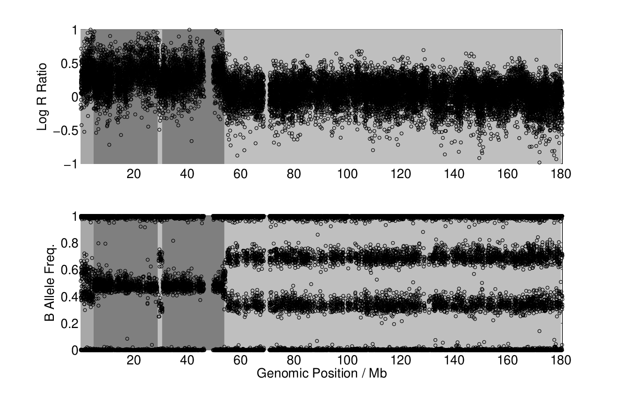
As an illustration, Figure 1 depicts a SNP genotyping dataset that measures variation in DNA copy number along a particular chromosome from DNA derived from tumour cells. The statistical problem is to divide the sequence up into regions and classify each region by the underlying DNA copy number. Many Hidden Markov model based methods have been developed for this task (see for example Zhao et al. [2004]; Marioni et al. [2006]; Colella et al. [2007]; Wang et al. [2007]; Korbel et al. [2007]; Cahan et al. [2008]; Guha et al. [2008]) but the copy number predictions reported are typically those of the most probable state sequence found using the Viterbi algorithm or the most probable set of marginal predictions using the forward-backward algorithm. We will show that for applications, such as copy number calling, standard approaches for reporting the hidden state sequence are not always entirely applicable to the problem and that a decision theoretic approach using Markov Loss functions maybe of greater utility and provide increased flexibilty.

2 Decision Theory

To begin we shall define some notation, let $x_{i}\in\{0,\ldots,S\}$ denote the true unobserved underlying state at the $i=1,\ldots,n$ locations, and $y_{i}$ the corresponding observation. The task is to obtain a prediction $\hat{x}=\{\hat{x}_{1},\ldots,\hat{x}_{n}\}$ given a statistical model $\pi(x|y)$ (for notational simplicity, we shall suppress the conditioning on $y$ in the following and refer to $\pi(x|y)$ as $\pi(x)$). In this paper, we focus on the case where $x$ forms an unobserved discrete Markov chain, however, we stress that our approach is generic and not dependent on this Markov condition.

Decision theory [Berger, 1985; Bernardo and Smith, 2000] provides an axiomatic framework for making optimal decisions via the principle of minimum expected loss (or maximum expected utility). In our problem the “decision” is the reporting of $\hat{x}$ from which a set of actions will be taken with associated losses based on the unknown true state of nature $x$. We encapsulate the forms of error into a loss function $l(\hat{x}|x)$ which quantifies the loss of taking actions on $\hat{x}$ when the true state of nature is $x$. The principle of minimum expected loss (MEL) prescribes one should report $\hat{x}$ as

$$\hat{x} = \arg\min_{\tilde{x}}E_{\pi(x)}[l(\tilde{x}|x)],$$

$$= \arg\min_{\tilde{x}}\sum_{x}l(\tilde{x}|x)\pi(x).$$

For example, one potential loss function is to use

$$l(\hat{x}|x)=\left\{\begin{array}[]{ll}0,&{\textrm{if }}\hat{x}\equiv x\\ 1,&{\textrm{otherwise}}\end{array}\right.$$ (1)

which leads to the reporting of the most probable joint state sequence $\hat{x}=\arg\max_{x}\pi(x)$. For Hidden Markov Models, the most probable joint state sequence can be computed using the Viterbi algorithm [Rabiner, 1989]. We shall refer to this as the global loss function as a constant penalty is incurred if the prediction is not completely correct. Alternately if we choose

$$l(\hat{x}|x)=\sum_{i}l(\hat{x}_{i}|x_{i})$$

with

$$l(\hat{x}_{i}|x_{i})=\left\{\begin{array}[]{ll}0,&{\textrm{if }}\hat{x}_{i}\equiv x_{i}\\ 1,&{\textrm{otherwise}}\end{array}\right.$$ (2)

then the MEL is the set of marginal predictions $\tilde{x}_{i}=\arg\max_{x_{i}}\sum_{x_{-i}}\pi(\{x_{i},x_{-i}\})$ where the summation is over $x_{-i}$, the state sequence other than $x_{i}$. We shall refer to this as the marginal loss function as it considers each location independently of the others. With Hidden Markov models, the marginal probabilities can be calculated exactly using the forward-backward algorithm [Rabiner, 1989].

3 Motivation

Consider the simulated data sequence in Figure 2(a) for a two-state Hidden Markov model which contains a region of elevated signal related to an underlying change in the hidden state. Figure 2(b-e) shows the true underlying state sequence and four different predictions of this state sequence. All of the predictions contain the same number of misclassifications; for example, Figure 2(c-e) contain the same number of false negatives (if we assume state 0 to be a null state such that the notion of a false negative applies). It is apparent though that the predicted sequences are qualitatively very different and could lead to quite different actions if decisions are taken upon them. For example, Figure 2(d) contains three non-null segments whilst Figure 2(e) contain two segments. It is clear therefore that simply counting the number of state mis-classifications is insufficient.

Figure 2: Sequence predictions. An example data set (a) and four predictions of the underlying state sequence (b-e). (Grey, solid) Predicted and (Black, dashed) true state sequence.

3.1 Problems with global and marginal loss functions

If we consider the global loss function in (1), this loss function assigns a penalty of one if the predicted sequence $\hat{x}$ is not exactly identical to the true sequence $x$. This loss function is extreme in the sense that no matter how many classification errors are made, the same penalty is incurred - it is an all-or-nothing approach. Furthermore, for this loss function the entirety of the sequence is important, the optimal prediction must be globally and locally correct. In contrast, the marginal loss function, defined in (2), ignores any form of local or global structure. It concentrates instead on penalising classification error at each location considered independently of others which is equivalent to stating that the overall loss is invariant to permutations of the sequence $\{\hat{x}_{i},x_{i}\}_{i=1}^{n}$. It is apparent that these two commonly used loss functions correspond to quite opposite extremes and neither scenario maybe appropriate in segmental classification problems.

For example, in many situations it is rare for errors to be completely intolerable, rather there are acceptable tolerance levels for error. Under these circumstances it would not be appropriate to use the global loss function in which the same penalty is incurred irrespective of how many errors are made in the prediction. Furthermore, if we are interested in the segmental classification of linear sequences and we expect dependencies between states at different locations, it does not seem appropriate to use a marginal loss function that considers classification error at each location independently of the others; see for example Figure 2 (c-e).

Nonetheless, the appeal of these loss functions is that the computation of the state sequence with minimum expected loss is often analytically tractable or simple to approximate with commonly used statistical models. With Hidden Markov Models, the Viterbi algorithm allows the most probable sequence sequence to be found whilst the forward-backward algorithm allows the marginal probabilities $\pi(x_{i})=\sum_{x_{-i}}\pi(x)$ to be calculated in a time which is linear in the length of the data sequence.

3.2 Example application

In the identification of DNA copy number alterations from aCGH or SNP genotyping data the reporting of the most probable copy number state sequence or the set of most probable marginal copy number predictions is commonplace. However, the loss functions defined by (1) and (2) do not necessarily encapsulate the types of error that need to be considered in practice.

A recent example of a statistical model-based approach for CNV discovery is QuantiSNP [Colella et al., 2007]. This uses a Bayesian Hidden Markov model framework to identify CNVs from Illumina SNP genotyping data. QuantiSNP applies the Viterbi algorithm to obtain a final copy number state sequence prediction after fitting the Hidden Markov model to the SNP data using an expectation-maximisation algorithm. Furthermore, QuantiSNP also assigns a measure of uncertainty to each putative CNV by calculating the Bayes Factor $\pi(\hat{x}_{i:j}=\mathrm{CNV}|y)/\pi(\hat{x}_{i:j}=\mathrm{NULL})$ which gives the ratio of the marginal probability that the region, spanned by the probes $i$ to $j$, contains a CNV to the marginal probability that the region does not contain a CNV. False positive CNV calls can be reduced by setting an appropriate threshold for the minimum acceptable Bayes Factor. This procedure though has a weakness in that it conditions on the Viterbi sequence.

Given a statistical model, the Viterbi algorithm will return the state sequence that has maximum probability and there will typically be only one such sequence. If an experimentalist wished to increase their power to detect CNVs and was willing to accept increased numbers of false positives it would not be possible to accommodate this as there is a presumption of a global loss function on the underlying copy number sequence. It may be possible to adopt a marginal loss function instead but, as we have already highlighted, the use of a marginal loss function seems inappropriate as it ignores local structure by classifying each probe independently yet the overall goal of the algorithm is to discover local structure due to copy number variation.

Other copy number detection methods, based on Hidden Markov models, such as dChip [Zhao et al., 2004], BioHMM [Marioni et al., 2006], PennCNV [Wang et al., 2007] and wuHMM [Cahan et al., 2008] also condition on the Viterbi sequence and are therefore subject to the same problem.

3.3 Markov Loss Function

It seems apparent that a more general loss function is required that sits in between the extremes of the global and marginal loss functions. One which takes into account some notion of local sequence structure whilst still remaining amenable to tractable computations.

Let us return to the predicted sequences in Figure 2. None of the four predictions depicted returns the true sequence and each sequence contains the same number of mis-classified locations; however, the predictions differ in the number of state transition errors and hence the number of segments reported. If we assume that one of the states can be considered to be a null or resting state, one approach, from the many possible, is to characterise four types of error in making the decision to switch from a state $\hat{x}_{i}=j$ to $\hat{x}_{i+1}\neq j$:

1.

$\hat{x}$ predicts a state transition where there is none. We refer to this as a False Positive Transition (FPT).

2.

$\hat{x}$ misses a state transition where one actually exists. We refer to this as a False Negative Transition (FNT).

3, 4.

$\hat{x}$ correctly predicts that there is no state transition but calls the incorrect state. We refer to these as False Positive Calls (FPC) and False Negative Calls (FNC) respectively.

There is also a fifth error type:

5.

$\hat{x}$ predicts a state transition in a direction that is opposite to the truth. We refer to these as Doubly False Transition (DFT). This is the most catastrophic error type when the predicted change point is structurally incompatible with the true changepoint. A high loss should be associated with this error.

We can now begin to differentiate the sequences in Figure 2(b, c) from those shown in Figure 2(d, e). Whilst Figure 2(b, c) each contain one pair of false positive and negative transition errors and report only one segment, those in Figure 2(d, e) consist of multiple transition errors and report a number of segments. In a CNV calling application, each state transition error corresponds to either a incorrectly specified breakpoint or a false putative CNV call and these errors carry implications for the cost of follow-up studies since each putative CNV (segment) might require further experimental validation.

The importance of state transition errors motivates the use of a loss function that assigns penalties to false state transition calls. We now propose a class of loss function that we will refer to as Markov Loss functions,

$$l(\hat{x}_{i,i+1}|x_{i,i+1})=\left\{\begin{array}[]{ll}0,&\hat{x}_{i,i+1}\equiv x_{i,i+1},\\ 1,&{\mathrm{otherwise}}\end{array}\right.$$ (3)

where $x_{i,i+1}=\{x_{i},x_{i+1}\}$. In the following section, we will describe how to calculate the expected loss for this novel class of loss function, as well a dynamic programming solution to obtain the sequence that has the minimum expected loss under this loss function.

4 Method

4.1 Calculating the Expected Loss under the Markov Loss function

Let $x$ be a state sequence, where $x_{i}\in\{0,\dots,S\},i=1,\dots,n$, and $S$ is the total number of possible states. The loss function $l(\hat{x}|x)$ shall consist of a sum of Markov loss functions that penalises transitions in $x$,

$$l(\hat{x}|x)=\sum_{i=1}^{n-1}l(\hat{x}_{i,i+1}|x_{i,i+1}).$$ (4)

The expected loss is given by,

$$E_{\pi(x)}[l(\tilde{x}|x)]=\sum_{x}\left\{\sum_{i=1}^{n-1}l(\tilde{x}_{i,i+1}|x_{i,i+1})\right\}\pi(x)$$ (5)

where, by exchanging the order of summation,

$$E_{\pi(x)}[l(\tilde{x}|x)] = \sum_{i=1}^{n-1}\left\{\sum_{x}l(\tilde{x}_{i,i+1}|x_{i,i+1})\pi(x)\right\},$$

$$= \sum_{i=1}^{n-1}\left\{\sum_{x_{i,i+1}}l(\tilde{x}_{i,i+1}|x_{i,i+1})\pi(x_{i,i+1})\right\}.$$

4.2 Dynamic Programming

As the expected loss for the Markov loss function is additive, the prediction $\hat{x}$ that has MEL can be found using the following dynamic programming recursions (in similar fashion to the Viterbi algorithm):

4.2.1 Forward recursion

Compute,

$$\phi_{1}(k) = \min_{j}E_{\pi(x_{1,2})}[l(\tilde{x}_{1,2}=(j,k)|x_{1,2})],$$

$$\delta_{1}(k) = \arg\min_{j}E_{\pi(x_{1,2})}[l(\tilde{x}_{1,2}=(j,k)|x_{1,2})],$$

where $k\in\{0,\dots,S\}$ and then for $i=2,\dots,n$,

$$\phi_{i}(k) = \min_{j}[\phi_{i-1}(j)+L(\tilde{x}_{i,i-1}=(j,k))],$$

$$\delta_{i}(k) = \arg\min_{j}[\phi_{i-1}(j)+L(\tilde{x}_{i,i-1}=(j,k))],$$

where $L(\tilde{x}_{i,i-1})=\sum_{x_{i,i-1}}l(\tilde{x}_{i,i-1}|x_{i,i-1})\pi(x_{i,i-1})$.

4.2.2 Backward trace

Find $\hat{x}_{n}=\arg\min_{k}\phi_{n}(k)$ then $\hat{x}_{i-1}=\delta_{i}(\hat{x}_{i}),i=n-1,\dots,2$.

4.3 Loss Matrix

For binary sequences ($S=1$), the loss matrix consists of $4\times 4=16$ elements, each corresponding to one of the possible prediction-truth state transitions. Table 1 shows one design of the loss matrix which consists of six unique loss values $C_{TP}$, $C_{FPC}$, $C_{FNC}$, $C_{FPT}$, $C_{FNT}$ and $C_{DFT}$. The value of $C_{TP}$ corresponds to the loss incurred with making the correct prediction which we normally set to zero, whilst the other loss values correspond to the penalties incurred for each of the transition errors described previously. It should be noted that the marginal loss function is a particular case of our Markov loss function when the losses associated with transition errors are zero $(C_{FPT}=C_{FNT}=0)$. For the global loss function, the loss matrix would consist of $2^{n}\times 2^{n}$ entries where each element corresponded to a different {prediction-truth} sequence pair with zeros on the diagonal and all ones on the off-diagonal elements.

Table 1: Loss matrix structure for binary state transitions.

$x$ $l(\tilde{x}|x)$ (0, 0) (0, 1) (1, 0) (1, 1) $\tilde{x}$ (0, 0) $C_{TP}$ $C_{FNT}+C_{FNC}$ $C_{FNT}$ $C_{FNC}$ (0, 1) $C_{FPT}+C_{FPC}$ $C_{TP}$ $C_{DFT}+C_{FPC}$ $C_{FPT}$ (1, 0) $C_{FPT}$ $C_{DFT}+C_{FNC}$ $C_{TP}$ $C_{FPT}+C_{FNC}$ (1, 1) $C_{FPC}+C_{FPC}$ $C_{FNT}$ $C_{FNT}+C_{FPC}$ $C_{TP}$

In our example application of CNV calling an appropriate loss matrix design would assign high loss to catastrophic doubly false transition errors $C_{DFT}\gg 1$ which corresponds to predicting the start of a CNV where a CNV region is actually ending. The values of the other loss parameters are study-dependent. In a CNV application, large values of $C_{FPC}$ and $C_{FPT}$ relative to $C_{FNC}$ and $C_{FNT}$ would lead to fewer misclassified probes and CNV calls as the penalities for false positive state classifications and transitions are severe. In contrast, relatively smaller values of $C_{FPC}$ and $C_{FPT}$ would encouraged the production of more putative CNV calls, and therefore increase the power to detect copy number variants albeit at the expense of an increase in false positive CNV calls.

One point of note is that the Markov loss function increases the number of free parameters that need to be specified. This additional parameterisation is necessary in order to obtain the flexibility that is often required in empirical data analysis. Careful design of the design matrix and consideration of the problem can minimise the number of free parameters. For example, in the loss matrix shown in Table 1, there are only three free parameters $C_{FNT}/C_{FPT}$, $C_{FNC}/C_{FPC}$ and $C_{FPT}/C_{FPC}$ once $C_{DFT}$ and $C_{TP}$ are given since the actual scale of the loss matrix does not matter.

4.4 Computational requirements

The order of computation required is ${\cal O}(S^{4}N)$, where $S$ is the number of hidden states in the Hidden Markov model and $N$ is the sequence length, since a summation is required over all possible pairs of the true hidden states $x_{i,i+1}$ and predictions $\hat{x}_{i,i+1}$. This can be prohibitive for applications involving large state spaces but is computationally manageable for small numbers of hidden states. In practical situations though it is often the case that the posterior probability distribution assigns high probabilities to a few transitions whilst the reminder have negligible probability. For data exhibiting sparse properties, these features can be exploited in order to derive approximate algorithms for inference in Hidden Markov models (see Siddiqi and Moore [2005]) that can offer substantial computational gains at the expense of little error if the assumption of sparseness hold.

4.5 Uncertainty in the statistical model

We have assumed throughout the availability of the exact statistical model $\pi(x|y)$. In general, of course, it is rare in practice to have access to the exact statistical model and instead the model is known up to a form $\pi(x,\theta|y)$ that includes some unknown model parameters $\theta$. The prediction must then satisfy,

$$\hat{x} =\arg\min_{z}\int_{\Theta}\left[\sum_{x\in\cal X}L(z;x)\pi(x,\theta|y)\right]d\theta,$$

$$=\arg\min_{z}\sum_{x\in\cal X}L(z;x)\pi(x|y),$$

$$\approx\arg\min_{z}\sum_{x\in\cal X}L(z;x)\hat{\pi}(x|y)$$

where, in the second line, the independence of the loss function and the model parameters allows $\theta$ to be integrated out of the model $\pi(x,\theta|y)$ and the problem is reduced to the same form as before. The integral required will generally be analytically intractable and an estimate $\hat{\pi}(x|y)$ must be used that can be obtained using Monte Carlo simulations, variational methods or by conditioning on point estimators (such as the MAP).

5 Results

5.1 Simulations

We performed a simulation study to examine the properties of predictions made by the use of global, marginal and Markov loss functions in a generic segmental classification setup.

5.1.1 Setup

We simulated 1000 data sequences of length $n=1000$ from a Hidden Markov Model with Gaussian observation densities,

$$\pi(y_{i}|x_{i},\mu,\sigma^{2}) = N(\mu_{x_{i}},\sigma^{2}),i=1,\dots,n,$$

$$\pi(x_{i}=j|x_{i-1}=k) = T(j,k),i=2,\dots,n,$$

$$\pi(x_{1}) = \nu(x_{1}),$$

where $\mu=\{0,1\}$, $\sigma^{2}=1$, the prior state vector $\nu=[0.5,0.5]^{T}$ and the transition matrix $T$ is given by,

$$T(j,k)=\left(\begin{array}[]{cc}1-\rho_{1}&\rho_{1}\\ \rho_{2}&1-\rho_{2}\end{array}\right),$$

with $\rho_{1}=0.01,\rho_{2}=0.05$. With probability $\eta=0.01$ we added outliers generated from a Gaussian distribution with mean $0$ and variance $3^{2}$.

For each simulated dataset, we used the Viterbi algorithm to find the most probable state sequence $\hat{x}_{v}$ and the forward-backward algorithm to obtain the marginal state and switching probabilities $\pi(x_{i}|y)$ and $\pi(x_{i,i+1}|y)$. Using a more generalised form of the marginal loss function,

$$l(\hat{x}_{i}|x_{i})=\left\{\begin{array}[]{ll}0,&\hat{x}_{i}\equiv x_{i},\\ C_{FPC},&\hat{x}_{i}=1,x_{i}=0,\\ C_{FNC},&\hat{x}_{i}=0,x_{i}=1,\end{array}\right.$$

in which the ratio $C_{FPC}/C_{FNC}$ allows us to control the Type I/II location-wise classification errors. We also obtained marginal loss predictions $\hat{x}_{m}$ with $C_{FNC}=1$ and values of $C_{FPC}$ from 0.1 to 10.

Sequence predictions $\hat{x}_{ml}$ were also obtained using the Markov loss function where we set $C_{DFT}=1000$ and explored a range of values for the ratios $C_{FPT}$ and $C_{FPC}$ from 0.1 to 10 with $C_{FNC}=C_{FNT}=1$.

5.1.2 Example simulated dataset

Figure 3: Analysis of simulated dataset. (a) Data containing jumps in signal intensity corresponding to underlying changes in the hidden state sequence (black). Predicted state sequences (grey, $\circ$) using the (b) Viterbi algorithm, (c) marginal loss function with $C_{FPC}=C_{FNC}=1$, (d) Markov loss function with $C_{FPT}=C_{FNT}=C_{FPC}=C_{FNC}=1$, (e) marginal loss function with $C_{FPC}=0.1$ and (f) Markov loss function with $C_{FPC}=0.1$. Arrows indicate false positive segments which are singletons or short segments. The average false positive call rate for (e) and (f) are the same.

Figure 3(a) shows one of the simulated data sets which contains a number of segmental alterations. In Figure 3(b, c), the Viterbi and Marginal Loss predictions, with unit losses, produce similar state sequence predictions. However, decreasing the cost of false positive calls allows the marginal loss prediction to recover more of the underlying state transitions at the cost of more false positives as shown in Figure 3(e). These false positives consist of multiple singletons or short segments that span just a few locations and are generally undesirable in segmental classification. Figure 3(d, f) shows the predicted state sequences using the Markov loss function. As the cost of false positive calls is reduced, the predictions are able to capture more of the underlying true state sequence without producing singletons or short segments. Predictions made under the marginal loss function can be expected to contain such features can be expected since local sequence structure is not considered whereas the Markov loss function explicitly considers state transition errors and avoids generating such features.

5.1.3 Average performance using the global and marginal loss functions

Figure 4: Performance on simulated data sets. Classification error rates for (a) non-breakpoint locations, (b-c) false positive and negative transition. Classification ($+$) Viterbi. ($\vartriangle$) Marginal Loss. ($\circ$) Markov Loss ($C_{FPT}=1$, $C_{FPC}$ variable), ($\times$) $C_{FPC}=1$ and $C_{FPT}$ variable.

Figure 4 shows overall classification performance, in terms of average rates of false positive and negative calls and transitions, on the simulated datasets using the Viterbi and marginal loss predictions. Since there are no free parameters associated with a global loss function, the performance using the Viterbi prediction is fixed and cannot be varied. In contrast, the marginal loss predictions are able to provide a continuum of different performance rates that depend on the relative values of the loss associated with false positive and negative state classifications.

Under the marginal loss function, as the relative magnitude of the loss associated with a false positive to a false negative call is increased, the false positive rate (% FPC) decreases, whilst the number of false negatives (% FNC) increases. This is expected behaviour since the relative penalty associated with false positive errors is increasing. However, we note that the Viterbi prediction is able to produce, at the same rate of false positive calls, far fewer false positive transitions (% FPT) than the marginal loss predictions. This is not unexpected since the global loss function, which the Viterbi prediction assumes, favours predictions that are structurally correct on a global and local scale. In contrast, the marginal loss function is ignorant of any structure and is more likely to produce state sequence predictions that contain small or even single location segments, thus contributing to an inflation in the rate of false positive transition errors as we saw in Figure 3.

5.1.4 Average performance using the Markov loss functions

Figure 4 shows the average classification performance using the Markov Loss function on the simulated datasets for fixed $C_{FPT}=1$ with $C_{FPC}$ varying and for fixed $C_{FPC}=1$ with $C_{FPT}$ varied. For fixed $C_{FPT}=1$, we observe that the predicted sequences using the marginal and Markov loss functions achieve similar false positive and false negative call rates based on the number of locations that are incorrectly called. However, at the same false positive call rate, the method based on the Markov loss function gives fewer false positive and negative transitions.

When $C_{FPC}=1$ and $C_{FPT}$ is varied, the performance of the Viterbi and marginal predictions are uniquely specified but we are able to control the rates of false transition error with the Markov loss function. Whilst there was relatively little change in the false positive transition rates when $C_{FPC}$ was varied, alterations to $C_{FPT}$ have a more pronounced effect on the numbers of false positive transitions. This is expected since $C_{FPT}$ is the loss associated with making false positive transition errors whilst $C_{FPC}$ primarily penalises errors in the classification of individual states.

One point of interest is that, at an FPC rate of approximately 2.2%, we notice that an appropriate choice of $C_{FPT}$ allows the predictions under the Markov Loss function to achieve similar performance to the Viterbi predictions. In contrast, it is not possible to access this level of performance using the marginal loss function no matter what changes are made to the loss parameters. This shows empirically that predictions, under the Markov loss function, do indeed allow us to access performance levels that span the range between that of the marginal loss and global loss functions.

5.2 Flexible CNV calling using SNP genotyping data

We compared CNV analysis using QuantiSNP using the original Viterbi algorithm and a modified version using the proposed method based on Markov Loss functions. We used SNP genotyping data, acquired from the Illumina HumanHap650Y SNP genotyping array, for the human individual NA15510 which has been previously well-studied in the CNV literature [Korbel et al., 2007; Scherer et al., 2007]. As there are no gold standard, fully characterised human genomes, in terms of CNV content, we measured performance by comparing CNV calls from both methods studied with CNV loci stored on the Database of Genomic Variants (DGV) [Iafrate et al., 2004]. CNV calls were not filtered by thresholding via the Bayes Factor uncertainty measure in QuantiSNP and performance was measured solely on the predicted state sequence. In order to apply the Markov loss function, we extracted marginal switching probability estimates $\pi(x_{i,i+1})$ from QuantiSNP and we explored a range of values for $C_{FPC}$ and $C_{FPT}$ as before.

QuantiSNP, with the original Viterbi copy number sequence predictions, produced 65 CNV calls of which 35 could be mapped on to CNV loci in the DGV as shown in Figure 5(a). With the Markov loss function, we were able to access a wider spectrum of performance by modifying the loss parameters as shown in Figure 5(b, c). What is of particular interest is that the predicted copy number sequences returned by the Viterbi method does not necessarily contain all the possible CNVs. For example, with the following loss parameters $C_{FPT}=0.1$ and $C_{FPC}=1$, the Markov loss method produces 215 CNV calls with 81 overlapping a CNV locus in the DGV. This suggests that there maybe a further 46 CNVs contained in the sample that were not identified from the Viterbi prediction but are accessible to the Markov loss-based method, if one is prepared to accept higher levels of false CNV calls.

The key point to emphasise here is that the use of the Markov loss functions gives a much more flexible approach for CNV data analysis and enables the experimenter to analyse their data subject to their own tolerances for the number of false positives and negatives not that imposed on them by the algorithm developer.

Figure 5: CNV analysis of individual NA15510 using QuantiSNP. (a) Number of CNV calls and matches to the Database of Genomic Variants (DGV) from the Viterbi prediction (+) and the Markov Loss prediction (x) for different loss parameters. The number of CNV calls using the Markov loss function based predictions when (b) as a function of the false positive call rate and (c) as a function of the false positive transition rate. The circled lines (o) indicate the total number of calls made whilst the dotted line ($\cdot$) indicates the corresponding number of calls which match an entry in the Database of Genomic Variants.

6 Discussion

Hidden Markov Models have a rich history dating back over 30 years in signal processing, finance and more recently genomics. Despite the enormous breadth of applications there are only two current approaches in the literature to calling the hidden state sequence, the Viterbi-based (MAP) or marginal state predictions. The Viterbi prediction lacks flexibility whilst the marginal predictions seem inappropriate for segmentation applications in which Hidden Markov models are frequently applied. Here, we have presented a state sequence prediction method that uses a class of Markov loss functions which is more appropriate loss function for the segmentation and classification of linear sequence data using Hidden Markov models. The method is simple but we show that in applications, such as CNV calling, it is more intuitive to consider the correct classification of state transitions rather than the entirety of the state sequence or of individual states. In these scenarios the Markov loss function can be more suitable than the global or marginal loss functions that are often used in real applications.

The calculation of the posterior expected loss with respect to a Markov loss function was shown to have a simple form and a dynamic programming algorithm was provided to compute the state sequence with the minimum expected loss. Although, the emphasis was on the Hidden Markov model, this method can be applied to any statistical model for the segmentation and classification of linear sequence data that can provide estimates of the marginal state transition probability $\pi(x_{i,i+1})$. Therefore it can be used to augment, without modification, many existing statistical methods for analyzing sequence data such as those based on semi-Markov models, change point methods [Fearnhead and Liu, 2007] or product partition models [Barry and Hartigan, 1992]. Whilst it is relatively simple addition the application of this method could greatly enhance the adaptability of many existing statistical algorithms transferring power to the experimenter to allow them to assign losses to various error types relevant to their own study.

Alternatives to maximum a posteriori estimators has been used in Hidden Markov model-based DNA segmentation applications by Aston and Martin [2007] and for clustering applications by Binder [1978] and Lau and Green [2007]. In particular, Lau and Green [2007] have argued that maximum a posteriori clustering estimates have no objective status in Bayesian theory as an “optimal” estimate of the data partition. Posterior modes can be unrepresentative of the centre of mass for the posterior distribution in high dimensional problems and point estimators should only be obtained after specifying some loss function and then computing the optimal parameter estimate that minimises the posterior expected loss.

Throughout this paper we have not explicitly stated how the loss values should be selected. This is purposeful because the selection of the costs associated with various error types is entirely study-dependent and it is only the data analyst who can develop the criteria for the design of the loss matrix. For example, in CNV analysis, costs might be related to tangible quantities such as the financial, time and man power requirements for follow-up studies and validation taken upon the predictions.

It is also of further research interest to characterise the effect on predictions when only an approximation of the statistical model is available. Furthermore, in some applications there maybe some utility in combining of Markov loss functions on the hidden state sequence $x$ and loss functions on the model parameters $\theta$. The Markov loss function introduced here focuses on costs associated with classification errors of the hidden state sequence and assumes that the model parameters are in some sense nuisance variables. There are applications where both the state sequence and model parameters maybe of interest; for example, the transition matrix may have some interpretation for a given application and a loss function maybe given on $\theta$. In these instances it maybe necessary to derive optimal joint predictions $(\hat{x},\hat{\theta})$ under the appropriate loss functions.

References

- Aston and Martin [2007] J. A. D. Aston and D. E. K. Martin. Distributions associated with general runs and patterns in Hidden Markov models. The Annals of Applied Statistics, 1(2):585–611, 2007.
- Banachewicz et al. [2008] K. Banachewicz, A. Lucas, and A. van der Vaart. Modelling Portfolio Defaults Using Hidden Markov Models with Covariates. Econometrics Journal, 11(1):155–171, 2008.
- Barry and Hartigan [1992] D. Barry and J. A. Hartigan. Product partition models for change point problems. Annals of Statistics, 20(1):260–279, 1992.
- Berger [1985] J.O. Berger. Statistical Decision Theory and Bayesian Analysis. Springer, 1985.
- Bernardo and Smith [2000] J. M Bernardo and A. F. M. Smith. Bayesian Theory. Wiley, 2000.
- Binder [1978] D. A. Binder. Bayesian Cluster Analysis. Biometrika, 65:31–38, 1978.
- Cahan et al. [2008] Patrick Cahan, Laura E Godfrey, Peggy S Eis, Todd A Richmond, Rebecca R Selzer, Michael Brent, Howard L McLeod, Timothy J Ley, and Timothy A Graubert. wuHMM: a robust algorithm to detect DNA copy number variation using long oligonucleotide microarray data. Nucleic Acids Res, 36(7):e41, 2008. URL http://dx.doi.org/10.1093/nar/gkn110.
- Chien and Furui [2005] J.T. Chien and S. Furui. Predictive hidden Markov model selection for speech recognition. Speech and Audio Processing, IEEE Transactions on, 13(3):377–387, 2005.
- Chopin and Pelgrin [2004] N. Chopin and F. Pelgrin. Bayesian inference and state number determination for hidden Markov models: an application to the information content of the yield curve about inflation. Journal of Econometrics, 123(2):327–344, 2004.
- Colella et al. [2007] Stefano Colella, Christopher Yau, Jennifer M Taylor, Ghazala Mirza, Helen Butler, Penny Clouston, Anne S Bassett, Anneke Seller, Christopher C Holmes, and Jiannis Ragoussis. QuantiSNP: an Objective Bayes Hidden-Markov Model to detect and accurately map copy number variation using SNP genotyping data. Nucleic Acids Res, 35(6):2013–2025, 2007. URL http://dx.doi.org/10.1093/nar/gkm076.
- Crowder et al. [2005] M. Crowder, M. Davis, and G. Giampieri. A hidden markov model of default interaction. Quantitative Finance, 5:27–34, 2005.
- Day et al. [2007] Nathan Day, Andrew Hemmaplardh, Robert E Thurman, John A Stamatoyannopoulos, and William S Noble. Unsupervised segmentation of continuous genomic data. Bioinformatics, 23(11):1424–1426, 2007. URL http://dx.doi.org/10.1093/bioinformatics/btm096.
- Egan et al. [2007] Chris M Egan, Srinath Sridhar, Michael Wigler, and Ira M Hall. Recurrent DNA copy number variation in the laboratory mouse. Nat Genet, 39(11):1384–1389, 2007. URL http://dx.doi.org/10.1038/ng.2007.19.
- Emerson et al. [2008] J. J. Emerson, Margarida Cardoso-Moreira, Justin O Borevitz, and Manyuan Long. Natural selection shapes genome-wide patterns of copy-number polymorphism in Drosophila melanogaster. Science, 320(5883):1629–1631, 2008. URL http://dx.doi.org/10.1126/science.1158078.
- Fearnhead and Liu [2007] P. Fearnhead and Z. Liu. Online Inference for Multiple Changepoint Problems. Journal of the Royal Statistical Society, Series B, 69:589–605, 2007.
- Guha et al. [2008] S. Guha, Y. Li, and D. Neuberg. Bayesian Hidden Markov Modeling of Array CGH Data. Journal of the American Statistical Association, 103:485–497, 2008.
- Iafrate et al. [2004] A. John Iafrate, Lars Feuk, Miguel N Rivera, Marc L Listewnik, Patricia K Donahoe, Ying Qi, Stephen W Scherer, and Charles Lee. Detection of large-scale variation in the human genome. Nat Genet, 36(9):949–951, 2004. URL http://dx.doi.org/10.1038/ng1416.
- Korbel et al. [2007] Jan O Korbel, Alexander Eckehart Urban, Fabian Grubert, Jiang Du, Thomas E Royce, Peter Starr, Guoneng Zhong, Beverly S Emanuel, Sherman M Weissman, Michael Snyder, and Mark B Gerstein. Systematic prediction and validation of breakpoints associated with copy-number variants in the human genome. Proc Natl Acad Sci U S A, 104(24):10110–10115, 2007. URL http://dx.doi.org/10.1073/pnas.0703834104.
- Lau and Green [2007] J. W. Lau and P. J. Green. Bayesian Model-Based Clustering Procedures. Journal of Computational & Graphical Statistics, 16 (3):526–558, 2007.
- Majoros et al. [2004] W. H. Majoros, M. Pertea, and S. L. Salzberg. TigrScan and GlimmerHMM: two open source ab initio eukaryotic gene-finders. Bioinformatics, 20(16):2878–2879, 2004. URL http://dx.doi.org/10.1093/bioinformatics/bth315.
- Marioni et al. [2006] J. C. Marioni, N. P. Thorne, and S. Tavaré. BioHMM: a heterogeneous hidden Markov model for segmenting array CGH data. Bioinformatics, 22(9):1144–1146, 2006. URL http://dx.doi.org/10.1093/bioinformatics/btl089.
- Pelham et al. [2006] Robert J Pelham, Linda Rodgers, Ira Hall, Robert Lucito, Ken C Q Nguyen, Nicholas Navin, James Hicks, David Mu, Scott Powers, Michael Wigler, and David Botstein. Identification of alterations in DNA copy number in host stromal cells during tumor progression. Proc Natl Acad Sci U S A, 103(52):19848–19853, 2006. URL http://dx.doi.org/10.1073/pnas.0609635104.
- Rabiner [1989] L. R. Rabiner. A tutorial on hidden Markov models and selected applications in speech recognition. In Proceedings of the IEEE, volume 77, pages 257–286, 1989.
- Redon et al. [2006] Richard Redon, Shumpei Ishikawa, Karen R Fitch, Lars Feuk, George H Perry, T. Daniel Andrews, Heike Fiegler, Michael H Shapero, Andrew R Carson, Wenwei Chen, Eun Kyung Cho, Stephanie Dallaire, Jennifer L Freeman, Juan R Gonzalez, Monica Gratacos, Jing Huang, Dimitrios Kalaitzopoulos, Daisuke Komura, Jeffrey R MacDonald, Christian R Marshall, Rui Mei, Lyndal Montgomery, Kunihiro Nishimura, Kohji Okamura, Fan Shen, Martin J Somerville, Joelle Tchinda, Armand Valsesia, Cara Woodwark, Fengtang Yang, Junjun Zhang, Tatiana Zerjal, Jane Zhang, Lluis Armengol, Donald F Conrad, Xavier Estivill, Chris Tyler-Smith, Nigel P Carter, Hiroyuki Aburatani, Charles Lee, Keith W Jones, Stephen W Scherer, and Matthew E Hurles. Global variation in copy number in the human genome. Nature, 444(7118):444–454, 2006. URL http://dx.doi.org/10.1038/nature05329.
- Rossi and Gallo [2006] A. Rossi and G.M. Gallo. Volatility estimation via hidden Markov models. Journal of Empirical Finance, 13(2):203–230, 2006.
- Scherer et al. [2007] Stephen W Scherer, Charles Lee, Ewan Birney, David M Altshuler, Evan E Eichler, Nigel P Carter, Matthew E Hurles, and Lars Feuk. Challenges and standards in integrating surveys of structural variation. Nat Genet, 39(7 Suppl):S7–15, 2007. URL http://dx.doi.org/10.1038/ng2093.
- Sebat et al. [2004] Jonathan Sebat, B. Lakshmi, Jennifer Troge, Joan Alexander, Janet Young, Par Lundin, Susanne Maner, Hillary Massa, Megan Walker, Maoyen Chi, Nicholas Navin, Robert Lucito, John Healy, James Hicks, Kenny Ye, Andrew Reiner, T. Conrad Gilliam, Barbara Trask, Nick Patterson, Anders Zetterberg, and Michael Wigler. Large-scale copy number polymorphism in the human genome. Science, 305(5683):525–528, 2004. URL http://dx.doi.org/10.1126/science.1098918.
- Sebat et al. [2007] Jonathan Sebat, B. Lakshmi, Dheeraj Malhotra, Jennifer Troge, Christa Lese-Martin, Tom Walsh, Boris Yamrom, Seungtai Yoon, Alex Krasnitz, Jude Kendall, Anthony Leotta, Deepa Pai, Ray Zhang, Yoon-Ha Lee, James Hicks, Sarah J Spence, Annette T Lee, Kaija Puura, Terho Lehtimaki, David Ledbetter, Peter K Gregersen, Joel Bregman, James S Sutcliffe, Vaidehi Jobanputra, Wendy Chung, Dorothy Warburton, Mary-Claire King, David Skuse, Daniel H Geschwind, T. Conrad Gilliam, Kenny Ye, and Michael Wigler. Strong association of de novo copy number mutations with autism. Science, 316(5823):445–449, 2007. URL http://dx.doi.org/10.1126/science.1138659.
- Siddiqi and Moore [2005] Sajid M. Siddiqi and Andrew W. Moore. Fast Inference and Learning in Large-State-Space HMMs. In Proceedings of the 22nd International Conference on Machine Learning, 2005.
- Stranger et al. [2007] Barbara E Stranger, Matthew S Forrest, Mark Dunning, Catherine E Ingle, Claude Beazley, Natalie Thorne, Richard Redon, Christine P Bird, Anna de Grassi, Charles Lee, Chris Tyler-Smith, Nigel Carter, Stephen W Scherer, Simon Tavare, Panagiotis Deloukas, Matthew E Hurles, and Emmanouil T Dermitzakis. Relative impact of nucleotide and copy number variation on gene expression phenotypes. Science, 315(5813):848–853, 2007. URL http://dx.doi.org/10.1126/science.1136678.
- Su et al. [2008] S.Y. Su, D.J. Balding, and L.J.M. Coin. Disease association tests by inferring ancestral haplotypes using a hidden markov model. Bioinformatics, 24(7):972, 2008.
- Wang et al. [2007] Kai Wang, Mingyao Li, Dexter Hadley, Rui Liu, Joseph Glessner, Struan F A Grant, Hakon Hakonarson, and Maja Bucan. PennCNV: an integrated hidden Markov model designed for high-resolution copy number variation detection in whole-genome SNP genotyping data. Genome Res, 17(11):1665–1674, Nov 2007. URL http://dx.doi.org/10.1101/gr.6861907.
- Weiss and Ellis [2008] R.J. Weiss and D.P.W. Ellis. Speech separation using speaker-adapted eigenvoice speech models. Computer Speech & Language, 2008.
- Xu et al. [2008] Bin Xu, J. Louw Roos, Shawn Levy, E. J. van Rensburg, Joseph A Gogos, and Maria Karayiorgou. Strong association of de novo copy number mutations with sporadic schizophrenia. Nat Genet, 40(7):880–885, 2008. URL http://dx.doi.org/10.1038/ng.162.
- Yan et al. [2007] Q. Yan, S. Vaseghi, E. Zavarehei, B. Milner, J. Darch, P. White, and I. Andrianakis. Formant tracking linear prediction model using HMMs and Kalman filters for noisy speech processing. Computer Speech & Language, 21(3):543–561, 2007.
- Zhao et al. [2004] Xiaojun Zhao, Cheng Li, J. Guillermo Paez, Koei Chin, Pasi A Janne, Tzu-Hsiu Chen, Luc Girard, John Minna, David Christiani, Chris Leo, Joe W Gray, William R Sellers, and Matthew Meyerson. An integrated view of copy number and allelic alterations in the cancer genome using single nucleotide polymorphism arrays. Cancer Res, 64(9):3060–3071, 2004.