Stabilization of a delayed quantum system:
the photon box case-studyThanks: This work was partially supported by the ”Agence Nationale de la Recherche” (ANR), ”Projet Blanc” CQUID number 06-3-13957 and ”Projet Jeunes Chercheurs” EPOQ2 number ANR-09-JCJC-0070.

Abstract

We study a feedback scheme to stabilize an arbitrary photon number state in a microwave cavity. The quantum non-demolition measurement of the cavity state allows a non-deterministic preparation of Fock states. Here, by the mean of a controlled field injection, we desire to make this preparation process deterministic. The system evolves through a discrete-time Markov process and we design the feedback law applying Lyapunov techniques. Also, in our feedback design we take into account an unavoidable pure delay and we compensate it by a stochastic version of a Smith predictor. After illustrating the efficiency of the proposed feedback law through simulations, we provide a rigorous proof of the global stability of the closed-loop system based on tools from stochastic stability analysis. A brief study of the Lyapunov exponents of the linearized system around the target state gives a strong indication of the robustness of the method.

1 Introduction

In the aim of achieving a robust processing of quantum information, one of the main tasks is to prepare and to protect various quantum states. Through the last 15 years, the application of quantum feedback paradigms has been investigated by many physicists [21, 19, 5, 10, 16] as a possible solution for this robust preparation. However, most (if not all) of these efforts have remained at a theoretical level and have not been able to be give rise to successful experiments. This is essentially due to the necessity of simulating, in parallel to the system, a quantum filter [1] providing an estimate of the state of the system based on the historic of quantum jumps induced by the measurement process. Indeed, it is, in general, difficult to perform such simulations in real time. In this paper, we consider a prototype of physical systems, the photon-box, where we actually have the time to perform these computations in real time (see [6] for a detailed description of this cavity quantum electrodynamics system).

Taking into account the measurement-induced quantum projection postulate, the most practical measurement protocols in the aim of feedback control are the quantum non-demolition (QND) measurements [2, 18, 20]. These are the measurements which preserve the value of the measured observable. Indeed, by considering a well-designed QND measurement process where the quantum state to be prepared is an eigenstate of the measurement operator, the measurement process, not only, is not an obstacle for the state preparation but can even help by adding some controllability.

In [4, 9, 8] QND measures are exploited to detect and/or produce highly non-classical states of light trapped in a super-conducting cavity (see [11, chapter 5] for a description of such QED systems and [3] for detailed physical models with QND measures of light using atoms). For such experimental setups, we detail and analyze here a feedback scheme that stabilizes the cavity field towards any photon-number states (Fock states). Such states are strongly non-classical since their photon numbers are perfectly defined. The control corresponds to a coherent light-pulse injected inside the cavity between atom passages. The overall structure of the proposed feedback scheme is inspired by [7] using a quantum adaptation of the observer/controller structure widely used for classical systems (see, e.g., [12, chapter 4]). As the measurement-induced quantum jumps and the controlled field injection happen in a discrete-in-time manner, the observer part of the proposed feedback scheme consists in a discrete-time quantum filter. Indeed, the discreteness of the measurement process provides us a first prototype of quantum systems where we, actually, have enough time to perform the quantum filtering and to compute the measurement-based feedback law to be applied as the controller.

From a mathematical modeling point of view, the quantum filter evolves through a discrete-time Markov chain. The estimated state is used in a state-feedback, based on a Lyapunov design. Indeed, by considering a natural candidate for the Lyapunov function, we propose a feedback law which ensures the decrease of its expectation over the Markov process. Therefore, the value of the considered Lyapunov function over the Markov chain defines a super-martingale. The convergence analysis of the closed-loop system is, therefore, based on some rather classical tools from stochastic stability analysis [13].

One of the particular features of the system considered in this paper corresponds to a non-negligible delay in the feedback process. In fact, in the experimental setup considered through this paper, we have to take into account a delay of $d$ steps between the measurement process and the feedback injection. Indeed, there are, constantly, $d$ atoms flying between the photon box (the cavity) to be controlled and the atom-detector (typically $d=5$). Therefore, in our feedback design, we do not have access to the measurement results for the $d$ last atoms. Through this paper, we propose an adaptation of the quantum filter, based on a stochastic version of the Smith predictor [17], which takes into account this delay by predicting the actual state of the system without having access to the result of $d$ last detections.

In the next section, we describe briefly the physical system and the associated quantum Monte-Carlo model. In Section 3, we consider the dynamics of the open-loop system. We will prove, through theorem 1 that the QND measurement process, without any additional controlled injection, allows a non-deterministic preparation of the Fock states. Indeed, we will see that the associated Markov chain converges, necessarily, towards a Fock state and that the probability of converging towards a fixed Fock state is given by its population over the initial state. Also, through proposition 1, we will show that the linearized open-loop system around a fixed Fock state admits strictly negative Lyapunov exponents (see Appendix B for a definition of the Lyapunov exponent).

In Section 4, we propose a Lyapunov-based feedback design allowing to stabilize globally the delayed closed-loop system around a desired Fock state. The theorem 2 proves the almost sure convergence of the trajectories of the closed-loop system towards the target Fock state. Also, through proposition 2, we will prove that the linearized closed-loop system around the target Fock state admits strictly negative Lyapunov exponents.

Finally in Section 5, we propose a brief discussion on the considered quantum filter and by proving a rather general separation principle (theorem 3), we will show a semi-global robustness with respect to the knowledge of the initial state of the system. Also, through a brief analysis of the linearized system-observer around the target Fock state and applying the propositions 1 and 2, we show that its largest Lyapunov exponent is also strictly negative (proposition 3).

A preliminary version of this paper without delay has appeared as a conference paper [15]. The delay compensation scheme is borrowed from [6]. The authors thank M. Brune, I. Dotsenko, S. Haroche and J.M. Raimond from ENS for many interesting discussions and advices.

2 A discrete-time Markov process

Figure 1: The quantum electrodynamic setup including the microwave cavity $C$ with its feedback scheme (in green).

As illustrated by Figure 1, the system consists in $C$ a high-Q microwave cavity, $B$ a box producing Rydberg atoms, $R_{1}$ and $R_{2}$ two low-Q Ramsey cavities, $D$ an atom detector and $S$ a microwave source. The dynamics model is discret in time and relies on quantum Monte-Carlo trajectories (see [11, chapter 4]). Each time-step indexed by the integer $k$ corresponds to atom number $k$ coming from $B$, submitted then to a first Ramsey $\pi/2$-pulse in $R_{1}$, crossing the cavity $C$ and being entangled with it, submitted to a second $\pi/2$-pulse in $R_{2}$ and finally being measured in $D$. The state of the cavity is associated to a quantized mode. The control corresponds to a coherent displacement of amplitude $\alpha\in{\mathbb{C}}$ that is applied via the micro-wave source $S$ between two atom passages.

In this paper we consider a finite dimensional approximation of this quantized mode and take a truncation to $n^{\text{\tiny max}}$ photons. Thus the cavity space is approximated by the Hilbert space ${\mathbb{C}}^{n^{\text{\tiny max}}+1}$. It admits $(\left|0\right>,\left|1\right>,\ldots,\left|n^{\text{\tiny max}}\right>)$ as ortho-normal basis. Each basis vector $\left|n\right>\in{\mathbb{C}}^{n^{\text{\tiny max}}+1}$ corresponds to a pure state, called Fock state, where the cavity has exactly $n$ photons, $n\in\{0,\ldots,n^{\text{\tiny max}}\}$. In this Fock-states basis the number operator N corresponds to the diagonal matrix

$${\text{\bf N}}=\text{diag}(0,1,\ldots,n^{\text{\tiny max}}).$$

The annihilation operator truncated to $n^{\text{\tiny max}}$ photons is denoted by a. It corresponds to the upper $1$-diagonal matrix filled with $(\sqrt{1},\ldots,\sqrt{n^{\text{\tiny max}}})$:

$${\text{\bf a}}\left|0\right>=0,\quad{\text{\bf a}}\left|n\right>=\sqrt{n}\left|n-1\right>\text{\penalty\ for\penalty\ }n=1,\ldots,n^{\text{\tiny max}}$$

The truncated creation operator denoted by ${\text{\bf a}}^{\dagger}$ is the Hermitian conjugate of a. Notice that we still have ${\text{\bf N}}={\text{\bf a}}^{\dagger}{\text{\bf a}}$, but truncation does not preserve the usual commutation $[{\text{\bf a}},{\text{\bf a}}^{\dagger}]=1$ that is only valid when $n^{\text{\tiny max}}=+\infty$.

Just after the measurement of the atom number $k-1$, the state of the cavity is described by the density matrix $\rho_{k}$ belonging to the following set of well-defined density matrices:

$${\mathcal{X}}=\left\{\rho\in{\mathbb{C}^{(n^{\text{\tiny max}}+1)^{2}}}\quad|\quad\rho=\rho^{\dagger},\penalty\ \text{Tr}\left(\rho\right)=1,\penalty\ \rho\geq 0\right\}.$$ (1)

The random evolution of this state $\rho_{k}$ can be modeled through a discrete-time Markov process that will be described bellow (see [6] and the references therein explaining the physical modeling assumptions).

Let us denote by $\alpha_{k}\in{\mathbb{C}}$ the control at step $k$. Then $\rho_{k+1}$, the cavity state after measurement of atom $k$ is given by

$$\rho_{k+1}={\mathbb{M}}_{s_{k}}(\rho_{k+\text{\scriptsize$\frac{1}{2}$}}),\quad\rho_{k+\text{\scriptsize$\frac{1}{2}$}}={\mathbb{D}}_{\alpha_{k-d}}(\rho_{k})$$ (2)

where,

• $s_{k}\in\{g,e\}$, ${\mathbb{M}}_{g}(\rho)=\tfrac{M_{g}\rho M_{g}^{\dagger}}{\text{Tr}\left(M_{g}\rho M_{g}^{\dagger}\right)}$, ${\mathbb{M}}_{e}(\rho)=\tfrac{M_{e}\rho M_{e}^{\dagger}}{\text{Tr}\left(M_{e}\rho M_{e}^{\dagger}\right)}$ with operators $M_{g}=\cos\left(\varphi_{0}+{\vartheta}{\text{\bf N}}\right)$ and $M_{e}=\sin\left(\varphi_{0}+{\vartheta}{\text{\bf N}}\right)$ ($\varphi_{0},{\vartheta}$ constant parameters). For any $n\in\{0,\ldots,n^{\text{\tiny max}}\}$ we set $\varphi_{n}=\varphi_{0}+n{\vartheta}$.

• ${\mathbb{D}}_{\alpha}(\rho)=D_{\alpha}\rho D_{\alpha}^{\dagger}$ where the unitary displacement operator $D_{\alpha}$ is given by $D_{\alpha}=e^{\alpha{\text{\bf a}}^{\dagger}-\alpha^{*}{\text{\bf a}}}.$ In open-loop, $\alpha=0$, $D_{0}={\mathbb{I}}$ (identity operator) and ${\mathbb{D}}_{0}(\rho)=\rho$. Notice that $D_{\alpha}^{\dagger}=D_{-\alpha}$.

• $s_{k}$ is a random variable taking the value $g$ when the atom $k$ is detected in $g$ (resp. $e$ when the atom $k$ is detected in $e$) with probability

  $$P_{g,k}=\text{Tr}\left(M_{g}\rho_{k+\text{\scriptsize$\frac{1}{2}$}}M_{g}^{\dagger}\right)\quad\left(\text{resp.}\penalty\ P_{e,k}=\text{Tr}\left(M_{e}\rho_{k+\text{\scriptsize$\frac{1}{2}$}}M_{e}^{\dagger}\right)\right).$$ (3)

• The control elaborated at step $k$, $\alpha_{k}$, is subject to a delay of $d$ steps, $d$ being the number of flying atoms between the cavity $C$ and the detector $D$.

We will assume through out the paper that the parameters $\varphi_{0}$, $\vartheta$ are chosen in order to have $M_{g}$, $M_{e}$ invertible and such that the spectrum of $M_{g}^{\dagger}M_{g}=M_{g}^{2}$ and $M_{e}^{\dagger}M_{e}=M_{e}^{2}$ are not degenerate. This implies that the nonlinear operators ${\mathbb{M}}_{g}$ and ${\mathbb{M}}_{e}$ are well defined for all $\rho\in{\mathcal{X}}$ and that ${\mathbb{M}}_{g}(\rho)$ and ${\mathbb{M}}_{e}(\rho)$ belongs also to the state space ${\mathcal{X}}$ defined by (1). Notice that $M_{g}$ and $M_{e}$ commute, are diagonal in the Fock basis and satisfy $M_{g}^{\dagger}M_{g}+M_{e}^{\dagger}M_{e}={\mathbb{I}}$. The Kraus map associated to this Markov process is given by:

$${\mathbb{K}}_{\alpha}(\rho)=M_{g}D_{\alpha}\rho D_{\alpha}^{\dagger}M_{g}^{\dagger}+M_{e}D_{\alpha}\rho D_{\alpha}^{\dagger}M_{e}^{\dagger}.$$ (4)

It corresponds to the expectation value of $\rho_{k+1}$ knowing $\rho_{k}$ and $\alpha_{k-d}$:

$${\text{\large$\mathbb{E}$}}\left(\rho_{k+1}\penalty\ |\penalty\ \rho_{k},\alpha_{k-d}\right)={\mathbb{K}}_{\alpha_{k-d}}(\rho_{k}).$$ (5)

3 Open loop dynamics

3.1 Simulations

Figure 2: $\left<3|\rho_{k}|3\right>$ (fidelity with respect to the $3$-photon state) versus the number of passing atoms $k\in\{0,\ldots,400\}$ for 100 realizations of the open-loop Markov process (6) (blue fine curves) starting from the same coherent state $\rho_{0}={\mathbb{D}}_{\sqrt{3}}(\left|0\right>\left<0\right|)$. The ensemble average over these realizations corresponds to the thick red curve.

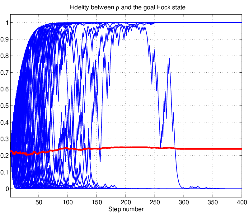
We consider in this section the following dynamics

$$\rho_{k+1}={\mathbb{M}}_{s_{k}}(\rho_{k}),$$ (6)

obtained from (2) when $\alpha_{k-d}\equiv 0$. Figure 2 corresponds to 100 realizations of this Markov process with $n^{\text{\tiny max}}=10$ photons, ${\vartheta}=\tfrac{2}{10}$ and $\varphi_{0}=\tfrac{\pi}{4}-3{\vartheta}$. For each realization, $\rho_{0}$ is initialized to the the same coherent state ${\mathbb{D}}_{\sqrt{3}}(\left|0\right>\left<0\right|)$ with $\text{Tr}\left({\text{\bf N}}\rho_{0}\right)\approx 3$ as mean photon number. We observe that either $\left<3|\rho_{k}|3\right>$ tends to $1$ or $0$. Since the ensemble average curve is almost constant, the proportion of trajectories for which $\left<3|\rho_{k}|3\right>$ tends to $1$ is given approximatively by $\left<3|\rho_{0}|3\right>$.

3.2 Global convergence analysis

The following theorem underlies the observations made for simulations of Figure 2

Theorem 1.

Consider the Markov process $\rho_{k}$ obeying (6) with an initial condition $\rho_{0}\in{\mathcal{X}}$ defined by (1). Then

• for any $n\in\{0,\cdots,n^{\text{\tiny max}}\}$, $\text{Tr}\left(\rho_{k}\left|n\right>\left<n\right|\right)=\left<n\right|\rho_{k}\left|n\right>$ is a martingale

• $\rho_{k}$ converges with probability $1$ to one of the $n^{\text{\tiny max}}+1$ Fock state $\left|n\right>\left<n\right|$ with $n\in\{0,\cdots,n^{\text{\tiny max}}\}$.

• the probability to converge towards the Fock state $\left|n\right>\left<n\right|$ is given by $\text{Tr}\left(\rho_{0}\left|n\right>\left<n\right|\right)=\left<n\right|\rho_{0}\left|n\right>$.

Proof.

Let us prove that $\text{Tr}\left(\rho_{k}\left|n\right>\left<n\right|\right)$ is a martingale. Set $\xi=\left|n\right>\left<n\right|$. We have

$${\text{\large$\mathbb{E}$}}\left(\text{Tr}\left(\xi\rho_{k+1}\right)\penalty\ |\penalty\ \rho_{k}\right)=P_{g,k}\text{Tr}\left(\xi\tfrac{M_{g}\rho_{k}M_{g}^{\dagger}}{P_{g,k}}\right)+P_{e,k}\text{Tr}\left(\xi\tfrac{M_{e}\rho_{k}M_{e}^{\dagger}}{P_{e,k}}\right)\\ =\text{Tr}\left(\xi M_{g}\rho_{k}M_{g}^{\dagger}\right)+\text{Tr}\left(\xi M_{e}\rho_{k}M_{e}^{\dagger}\right)=\text{Tr}\left(\rho_{k}(M^{\dagger}_{g}\xi M_{g}+M_{e}^{\dagger}\xi M_{e})\right).$$

Since $\xi$ commutes with $M_{g}$ and $M_{e}$ and $M^{\dagger}_{g}M_{g}+M^{\dagger}_{e}M_{e}={\mathbb{I}}$ we have ${\text{\large$\mathbb{E}$}}\left(\text{Tr}\left(\xi\rho_{k+1}\right)\penalty\ |\penalty\ \rho_{k}\right)=\text{Tr}\left(\xi\rho_{k}\right)$.

Considering the following function:

$$V_{n}(\rho)=f(\left<n|\rho|n\right>),$$

where $f(x)=\tfrac{x+x^{2}}{2}.$ Notice that $f$ is $1$-convexe, $f^{\prime}\geq\tfrac{1}{2}$ on $[0,1]$ and satisfies

$$\forall(x,y,\theta)\in[0,1],\quad\theta f(x)+(1-\theta)f(y)=\tfrac{\theta(1-\theta)}{2}(x-y)^{2}+f(\theta x+(1-\theta)y).$$ (7)

The function $f$ is increasing and convex and $\left<n|\rho_{k}|n\right>$ is a martingale. Thus $V_{n}(\rho_{k})$ is sub-martingale. Since

$$\left<n|{\mathbb{M}}_{g}(\rho)|n\right>=\tfrac{\cos^{2}\!\varphi_{n}}{\text{Tr}\left(M_{g}\rho M_{g}^{\dagger}\right)}\left<n|\rho|n\right>,\quad\left<n|{\mathbb{M}}_{e}(\rho)|n\right>=\tfrac{\sin^{2}\!\varphi_{n}}{\text{Tr}\left(M_{e}\rho M_{e}^{\dagger}\right)}\left<n|\rho|n\right>$$

we have

$${\text{\large$\mathbb{E}$}}\left(V_{n}(\rho_{k+1})\penalty\ |\penalty\ \rho_{k}\right)=\text{Tr}\left(M_{g}\rho_{k}M_{g}^{\dagger}\right)f\left(\tfrac{\cos^{2}\!\varphi_{n}}{\text{Tr}\left(M_{g}\rho_{k}M_{g}^{\dagger}\right)}\left<n|\rho_{k}|n\right>\right)\\ +\text{Tr}\left(M_{e}\rho_{k}M_{e}^{\dagger}\right)f\left(\tfrac{\sin^{2}\!\varphi_{n}}{\text{Tr}\left(M_{e}\rho_{k}M_{e}^{\dagger}\right)}\left<n|\rho_{k}|n\right>\right)$$

Then (7), together with

$$\theta=\text{Tr}\left(M_{g}\rho_{k}M_{g}^{\dagger}\right),\penalty\ x=\tfrac{\cos^{2}\!\varphi_{n}}{\text{Tr}\left(M_{g}\rho_{k}M_{g}^{\dagger}\right)}\left<n|\rho_{k}|n\right>,\penalty\ y=\tfrac{\sin^{2}\!\varphi_{n}}{\text{Tr}\left(M_{e}\rho_{k}M_{e}^{\dagger}\right)}\left<n|\rho_{k}|n\right>$$

yields to

$${\text{\large$\mathbb{E}$}}\left(V_{n}(\rho_{k+1})\penalty\ |\penalty\ \rho_{k}\right)-V_{n}(\rho_{k})=\\ \tfrac{\text{Tr}\left(M_{g}\rho_{k}M_{g}^{\dagger}\right)\text{Tr}\left(M_{e}\rho_{k}M_{e}^{\dagger}\right)(\left<n|\rho_{k}|n\right>)^{2}}{2}\left(\tfrac{\cos^{2}\!\varphi_{n}}{\text{Tr}\left(M_{g}\rho_{k}M_{g}^{\dagger}\right)}-\tfrac{\sin^{2}\!\varphi_{n}}{\text{Tr}\left(M_{e}\rho_{k}M_{e}^{\dagger}\right)}\right)^{2}.$$

Thus we recover that $V_{n}(\rho_{k})$ is a sub-martingale, ${\text{\large$\mathbb{E}$}}\left(V_{n}(\rho_{k+1})\penalty\ |\penalty\ \rho_{k}\right)\geq V_{n}(\rho_{k})$. We have also shown that ${\text{\large$\mathbb{E}$}}\left(V_{n}(\rho_{k+1})\penalty\ |\penalty\ \rho_{k}\right)=V_{n}(\rho_{k})$ implies that either $\left<n|\rho_{k}|n\right>=0$ or $\text{Tr}\left(M_{g}\rho_{k}M_{g}^{\dagger}\right)=\cos^{2}\!\varphi_{n}$ (assumption $M_{g}$ and $M_{e}$ invertible is used here).

We apply now the invariance theorem established by Kushner [13] (recalled in the Appendix A) for the Markov process $\rho_{k}$ and the sub-martingale $V_{n}(\rho_{k})$. This theorem implies that the Markov process $\rho_{k}$ converges in probability to the largest invariant subset of

$$\left\{\rho\in{\mathcal{X}}\penalty\ |\penalty\ \text{Tr}\left(M_{g}\rho M_{g}^{{\dagger}}\right)=\cos^{2}\!\varphi_{n}\text{ or }\left<n|\rho|n\right>=0\right\}.$$

But the set $\left\{\rho\in{\mathcal{X}}\penalty\ |\penalty\ \left<n|\rho|n\right>=0\right\}$ is invariant. It remains thus to characterized the largest invariant subset denoted by ${\mathcal{X}}_{n}$ and included in $\left\{\rho\in{\mathcal{X}}\penalty\ |\penalty\ \text{Tr}\left(M_{g}\rho M_{g}^{{\dagger}}\right)=\cos^{2}\!\varphi_{n}\right\}$.

Take $\rho\in{\mathcal{X}}_{n}$. Invariance means that ${\mathbb{M}}_{g}(\rho)$ and ${\mathbb{M}}_{e}(\rho)$ belong to ${\mathcal{X}}_{n}$ (the fact that $M_{g}$ and $M_{e}$ are invertible ensures that probabilities to jump with $s=g$ or $s=e$ are strictly positive for any $\rho\in{\mathcal{X}}$). Consequently $\text{Tr}\left(M_{g}{\mathbb{M}}_{g}(\rho)M_{g}^{\dagger}\right)=\text{Tr}\left(M_{g}\rho M_{g}^{{\dagger}}\right)=\cos^{2}\!\varphi_{n}$. This means that $\text{Tr}\left(M_{g}^{4}\rho\right)=\text{Tr}^{2}\left(M_{g}^{2}\rho\right)$. By Cauchy-Schwartz inequality,

$$\text{Tr}\left(M_{g}^{4}\rho\right)=\text{Tr}\left(M_{g}^{4}\rho\right)\text{Tr}\left(\rho\right)\geq\text{Tr}^{2}\left(M_{g}^{2}\rho\right)$$

with equality if, and only if, $M_{g}^{4}\rho$ and $\rho$ are co-linear. $M_{g}^{4}$ being non-degenerate, $\rho$ is necessarily a projector over an eigenstate of $M_{g}^{4}$, i.e., $\rho=\left|m\right>\left<m\right|$ for some $m\in\{0,\ldots,n^{\text{\tiny max}}\}$. Since $\text{Tr}\left(M_{g}\rho M_{g}^{{\dagger}}\right)=\cos^{2}\!\varphi_{n}>0$, $m=n$ and thus ${\mathcal{X}}_{n}$ is reduced to $\{\left|n\right>\left<n\right|\}$. Therefore the only possibilities for the $\omega$-limit set are $\text{Tr}\left(\rho\left|n\right>\left<n\right|\right)=0$ or $1$ and

$$W_{n}(\rho_{k})=\text{Tr}\left(\rho_{k}\left|n\right>\left<n\right|\right)(1-\text{Tr}\left(\rho_{k}\left|n\right>\left<n\right|\right)\stackrel{{\scriptstyle k\rightarrow\infty}}{{\longrightarrow}}0\qquad\text{in probability.}$$

The convergence in probability together with the fact that $W_{n}(\rho_{k})$ is a positive bounded ($W_{n}\in[0,1]$) random process implies the convergence in expectation. Indeed

$$\limsup_{k\rightarrow\infty}{\text{\large$\mathbb{E}$}}\left(W_{n}(\rho_{k})\right) \leq\epsilon\limsup_{k\rightarrow\infty}{\text{\large$\mathbb{P}$}}\left(W_{n}(\rho_{k})\leq\epsilon\right)+\limsup_{k\rightarrow\infty}{\text{\large$\mathbb{P}$}}\left(W_{n}(\rho_{k})>\epsilon\right)$$

$$\leq\epsilon+\limsup_{k\rightarrow\infty}{\text{\large$\mathbb{P}$}}\left(W_{n}(\rho_{k})>\epsilon\right)\leq\epsilon,$$

where for the last inequality, we have applied the convergence in probability of $W_{n}(\rho_{k})$ towards $0$. As the above inequality is valid for any $\epsilon>0$, we have

$$\lim_{k\rightarrow\infty}{\text{\large$\mathbb{E}$}}\left(W_{n}(\rho_{k})\right)=0.$$

Furthermore, by the first part of the Theorem, we know that $\text{Tr}\left(\rho_{k}\left|n\right>\left<n\right|\right)$ is a bounded martingale and therefore by the Doob’s first martingale convergence theorem (see the Theorem 4 of the Appendix A), $\text{Tr}\left(\rho_{k}\left|n\right>\left<n\right|\right)$ converges almost surely towards a random variable $l_{n}^{\infty}\in[0,1]$. This implies that $W_{n}(\rho_{k})$ converges almost surely towards the random variable $l_{n}^{\infty}(1-l_{n}^{\infty})\in[0,1]$. We apply now the dominated convergence theorem

$${\text{\large$\mathbb{E}$}}\left(l_{n}^{\infty}(1-l_{n}^{\infty})\right)={\text{\large$\mathbb{E}$}}\left(\lim_{k\rightarrow\infty}W_{n}(\rho_{k})\right)=\lim_{k\rightarrow\infty}{\text{\large$\mathbb{E}$}}\left(W_{n}(\rho_{k})\right)=0.$$

This implies that $l_{n}^{\infty}(1-l_{n}^{\infty})$ vanishes almost surely and therefore

$$W_{n}(\rho_{k})=\text{Tr}\left(\rho_{k}\left|n\right>\left<n\right|\right)(1-\text{Tr}\left(\rho_{k}\left|n\right>\left<n\right|\right))\stackrel{{\scriptstyle k\rightarrow\infty}}{{\longrightarrow}}0\qquad\text{almost surely.}$$

As we can repeat this same analysis for any choice of $n\in\{0,1,\ldots,n^{\text{\tiny max}}\}$, $\rho_{k}$ converges almost surely to the set of of Fock states

$$\{\left|n\right>\left<n\right|\penalty\ |\penalty\ n=0,1,\ldots,n^{\text{\tiny max}}\},$$

which ends the proof of the second part.

We have shown that the probability measure associated to the random variable $\rho_{k}$ converges to the probability measure

$$\sum_{n=0}^{n^{\text{\tiny max}}}p_{n}\delta(\left|n\right>\left<n\right|),$$

where $\delta(\left|n\right>\left<n\right|)$ denotes the Dirac distribution at $\left|n\right>\left<n\right|$ and $p_{n}$ is the probability of convergence towards $\left|n\right>\left<n\right|$. In particular, we have

$${\text{\large$\mathbb{E}$}}\left(\text{Tr}\left(\left|n\right>\left<n\right|\rho_{k}\right)\right)\stackrel{{\scriptstyle k\rightarrow\infty}}{{\longrightarrow}}p_{n}.$$

But $\text{Tr}\left(\left|n\right>\left<n\right|\rho_{k}\right)$ is a martingale and ${\text{\large$\mathbb{E}$}}\left(\text{Tr}\left(\left|n\right>\left<n\right|\rho_{k}\right)\right)={\text{\large$\mathbb{E}$}}\left(\text{Tr}\left(\left|n\right>\left<n\right|\rho_{0}\right)\right)$. Thus

$$p_{n}=\left<n\right|\rho_{0}\left|n\right>,$$

which ends the proof of the third and last part.

∎

3.3 Local convergence rate

According to theorem 1, the $\Omega$-limit set of the Markov process (6) is the discrete set of Fock states $\{\left|n\right>\left<n\right|\}_{n\in\{0,\ldots,n^{\text{\tiny max}}\}}$. We investigate here the local convergence rate around one of these Fock states denoted by $\bar{\rho}=\left|\bar{n}\right>\left<\bar{n}\right|$ for some $\bar{n}\in\{0,\ldots,n^{\text{\tiny max}}\}$.

Since ${\mathbb{M}}_{g}(\bar{\rho})={\mathbb{M}}_{e}(\bar{\rho})=\bar{\rho}$, we can develop the dynamics (6) around the fixed point $\bar{\rho}$. We write $\rho=\bar{\rho}+\delta\rho$ with $\delta\rho$ small, Hermitian and with zero trace. Keeping only the first order terms in (6), we have

$$\delta\rho_{k+1}=\tfrac{M_{s_{k}}\delta\rho_{k}M_{s_{k}}^{\dagger}}{\text{Tr}\left(M_{s_{k}}\bar{\rho}M_{s_{k}}^{\dagger}\right)}-\tfrac{\text{Tr}\left(M_{s_{k}}\delta\rho_{k}M_{s_{k}}^{\dagger}\right)}{\text{Tr}\left(M_{s_{k}}\bar{\rho}M_{s_{k}}^{\dagger}\right)}\bar{\rho}.$$

Thus the linearized Markov process around the fixed point $\bar{\rho}$ reads

$$\delta\rho_{k+1}=A_{s_{k}}\delta\rho_{k}A_{s_{k}}^{\dagger}-\text{Tr}\left(A_{s_{k}}\delta\rho_{k}A_{s_{k}}^{\dagger}\right)\bar{\rho}$$ (8)

where the random matrices $A_{s_{k}}$ are given by :

• $A_{g}=\frac{M_{g}}{\cos\varphi_{\bar{n}}}$ with probability $P_{g}=\cos^{2}\!\varphi_{\bar{n}}$

• $A_{e}=\frac{M_{e}}{\sin\varphi_{\bar{n}}}$ with probability $P_{e}=\sin^{2}\!\varphi_{\bar{n}}$.

The following proposition shows that the convergence of the linearized dynamics is exponential (a crucial robustness indication).

Proposition 1.

Consider the linear Markov chain (8) of state $\delta\rho$ belonging to the set of Hermitian matrices with zero trace. Then the largest Lyapunov exponent $\Lambda$ is given by ($\varphi_{n}=\varphi_{0}+n{\vartheta}$)

$$\Lambda=\max_{\text{\scriptsize$\begin{array}[]{c}n\in\{0,\ldots,n^{\text{\tiny max}}\}\\ n\neq\bar{n}\end{array}$}}\left(\cos^{2}\!\varphi_{\bar{n}}\log\left(\tfrac{|\cos\varphi_{n}|}{|\cos\varphi_{\bar{n}}|}\right)+\sin^{2}\!\varphi_{\bar{n}}\log\left(\tfrac{|\sin\varphi_{n}|}{|\sin\varphi_{\bar{n}}|}\right)\right)$$

and is strictly negative: $\Lambda<0$.

Proof.

Set $\delta\rho^{n_{1},n_{2}}=\left<n_{1}|\delta\rho|n_{2}\right>$ for any $n_{1},n_{2}\in\{0,\ldots,n^{\text{\tiny max}}\}$. Since $\text{Tr}\left(\delta\rho_{k}\right)\equiv 0$, we exclude here the case $(n_{1},n_{2})=(\bar{n},\bar{n})$ because $\delta\rho_{k}^{\bar{n},\bar{n}}=-\sum_{n\neq\bar{n}}\delta\rho_{k}^{n,n}$. Since $A_{e}$ and $A_{g}$ are diagonal matrices, we have

$$\delta\rho_{k+1}^{n_{1},n_{2}}=a_{s_{k}}^{n_{1},n_{2}}\delta\rho_{k}^{n_{1},n_{2}}$$ (9)

where $s_{k}=g$ (resp. $s_{k}=e$) with probability $\cos^{2}\varphi_{\bar{n}}$ (resp. $\sin^{2}\varphi_{\bar{n}}$) and where $a_{g}^{n_{1},n_{2}}=\tfrac{\cos\varphi_{n_{1}}\cos\varphi_{n_{2}}}{\cos^{2}\varphi_{\bar{n}}}$ and $a_{e}^{n_{1},n_{2}}=\tfrac{\sin\varphi_{n_{1}}\sin\varphi_{n_{2}}}{\sin^{2}\varphi_{\bar{n}}}$.

Denote by $\Lambda^{n_{1},n_{2}}$ the Lyapunov exponent of (9) for $(n_{1},n_{2})\neq(\bar{n},\bar{n})$. By the law of large numbers, we know that $\frac{\log\left(\left|\prod_{l=0}^{l=k}a_{s_{k}}^{n_{1},n_{2}}\right|\right)}{k+1}$ converges almost surely towards

$$\cos^{2}\!\varphi_{\bar{n}}\penalty\ \log(|a_{g}^{n_{1},n_{2}}|)+\sin^{2}\!\varphi_{\bar{n}}\penalty\ \log(|a_{e}^{n_{1},n_{2}}|).$$

Thus, we have

$$\Lambda^{n_{1},n_{2}}=\cos^{2}\varphi_{\bar{n}}\left(\log\left(\tfrac{|\cos\varphi_{n_{1}}|}{|\cos\varphi_{\bar{n}}|}\right)+\log\left(\tfrac{|\cos\varphi_{n_{2}}|}{|\cos\varphi_{\bar{n}}|}\right)\right)\\ +\sin^{2}\varphi_{\bar{n}}\left(\log\left(\tfrac{|\sin\varphi_{n_{1}}|}{|\sin\varphi_{\bar{n}}|}\right)+\log\left(\tfrac{|\sin\varphi_{n_{2}}|}{|\sin\varphi_{\bar{n}}|}\right)\right)$$

The function

$$\left[0,\frac{\pi}{2}\right]\ni\varphi\mapsto\left(\frac{\cos\varphi}{|\cos\varphi_{\bar{n}}|}\right)^{\cos^{2}\varphi_{\bar{n}}}\penalty\ \left(\frac{\sin\varphi}{|\sin\varphi_{\bar{n}}|}\right)^{\sin^{2}\varphi_{\bar{n}}}$$

increases strictly from $0$ to $1$ when $\varphi$ goes from $0$ to $\arcsin(|\sin\varphi_{\bar{n}}|)$ and decreases strictly from $1$ to $0$ when $\varphi$ goes from $\arcsin(|\sin\varphi_{\bar{n}}|)$ to $\frac{\pi}{2}$. Since $(n_{1},n_{2})\neq(\bar{n},\bar{n})$, $\Lambda^{n_{1},n_{2}}<0$. Denote by $\Lambda^{n}=\Lambda^{n,\bar{n}}$ for $n\in\{0,\ldots,n^{\text{\tiny max}}\}$:

$$\Lambda^{n}=\cos^{2}\!\varphi_{\bar{n}}\log\left(\tfrac{|\cos\varphi_{n}|}{|\cos\varphi_{\bar{n}}|}\right)+\sin^{2}\!\varphi_{\bar{n}}\log\left(\tfrac{|\sin\varphi_{n}|}{|\sin\varphi_{\bar{n}}|}\right).$$

Since $(n_{1},n_{2})\neq(\bar{n},\bar{n})$, we have $\Lambda^{n_{1},n_{2}}\leq\max_{n\neq\bar{n}}\Lambda^{n}$ and $\Lambda=\max_{n\neq\bar{n}}\Lambda^{n}$ is strictly negative. ∎

4 Feedback stabilization with delays

4.1 Feedback scheme and closed-loop simulations

Figure 3: $\text{Tr}\left(\rho_{k}\bar{\rho}\right)=\left<3|\rho_{k}|3\right>$ versus $k\in\{0,\ldots,400\}$ for 100 realizations of the closed-loop Markov process (2) with feedback (10) (blue fine curves) starting from the same state $\rho_{0}={\mathbb{D}}_{\sqrt{3}}(\left|0\right>\left<0\right|)$ (no delay, $d=0$). The ensemble average over these realizations corresponds to the thick red curve.

Figure 4: $\text{Tr}\left(\rho_{k}\bar{\rho}\right)=\left<3|\rho_{k}|3\right>$ versus $k\in\{0,\ldots,400\}$ for 100 realizations of the closed-loop Markov process (12) with feedback (11) (blue fine curves) starting from the same state $\chi_{0}=({\mathbb{D}}_{\sqrt{3}}(\left|0\right>\left<0\right|),0,\ldots,0)$ and with $5$-step delay ($d=5$). The ensemble average over these realizations corresponds to the thick red curve.

Through out this section we assume that we have access at each step $k$ to the cavity state $\rho_{k}$. The goal is to design a causal feedback law that stabilizes globally the Markov chain (2) towards a goal Fock state $\bar{\rho}=\left|\bar{n}\right>\left<\bar{n}\right|$ with $\bar{n}$ photon(s), $\bar{n}\in\{0,\ldots,n^{\text{\tiny max}}\}$. To be consistent with truncation to $n^{\text{\tiny max}}$ photons, $\bar{n}$ has to be far from $n^{\text{\tiny max}}$ (typically $\bar{n}=3$ with $n^{\text{\tiny max}}=10$ in the simulations below).

The feedback is based on the fact that, in open-loop when $\alpha_{k}\equiv 0$, $\text{Tr}\left(\bar{\rho}\rho_{k}\right)=\left<\bar{n}|\rho_{k}|\bar{n}\right>$ is a martingale. When $d=0$, [15] proves global almost sure convergence of the following feedback law

$$\alpha_{k}=\left\{\begin{array}[]{ll}\epsilon\text{Tr}\left(\bar{\rho}\penalty\ [\rho_{k},{\text{\bf a}}]\right)&\mbox{ if }\text{Tr}\left(\bar{\rho}\rho_{k}\right)\geq\eta\\ \underset{|\alpha|\leq\bar{\alpha}}{\text{argmax}}\left(\text{Tr}\left(\bar{\rho}\penalty\ {\mathbb{D}}_{\alpha}(\rho_{k})\right)\right)&\mbox{ if }\text{Tr}\left(\bar{\rho}\rho_{k}\right)<\eta\\ \end{array}\right.$$ (10)

for any $\bar{\alpha}>0$ when $\epsilon,\eta>0$ are small enough. This feedback law ensures that $\text{Tr}\left(\bar{\rho}\rho_{k}\right)$ is a sub-martingale.

When $d>0$, we cannot set $\alpha_{k-d}=\epsilon\text{Tr}\left(\bar{\rho}\penalty\ [\rho_{k},{\text{\bf a}}]\right)$ since $\alpha_{k}$ will depend on $\rho_{k+d}$ and the feedback law is not causal. In [6], this feedback law is made causal by replacing $\rho_{k+d}$ by its expectation value (average prediction) $\rho^{\text{\tiny pred}}_{k}$ knowing $\rho_{k}$ and the past controls $\alpha_{k-1}$, …, $\alpha_{k_{d}}$:

$$\rho^{\text{\tiny pred}}_{k}={\mathbb{K}}_{\alpha_{k-1}}\circ\ldots\circ{\mathbb{K}}_{\alpha_{k-d}}(\rho_{k})$$

where the Kraus map ${\mathbb{K}}_{\alpha}$ is defined by (4).

We will thus consider here the following causal feedback based on an average compensation of the delay $d$

$$\alpha_{k}=\left\{\begin{array}[]{ll}\epsilon\text{Tr}\left(\bar{\rho}\penalty\ [\rho^{\text{\tiny pred}}_{k},{\text{\bf a}}]\right)&\mbox{ if }\text{Tr}\left(\bar{\rho}\rho^{\text{\tiny pred}}_{k}\right)\geq\eta\\ \underset{|\alpha|\leq\bar{\alpha}}{\text{argmax}}\left(\text{Tr}\left(\bar{\rho}\penalty\ {\mathbb{D}}_{\alpha}(\rho^{\text{\tiny pred}}_{g,k})\right)\text{Tr}\left(\bar{\rho}\penalty\ {\mathbb{D}}_{\alpha}(\rho^{\text{\tiny pred}}_{e,k})\right)\right)&\mbox{ if }\text{Tr}\left(\bar{\rho}\rho^{\text{\tiny pred}}_{k}\right)<\eta\\ \end{array}\right.$$ (11)

with

$$\left\{\begin{array}[]{l}\rho^{\text{\tiny pred}}_{g,k}={\mathbb{K}}_{\alpha_{k-1}}\circ\ldots\circ{\mathbb{K}}_{\alpha_{k-d+1}}(M_{g}D_{\alpha_{k-d}}\rho_{k}D_{\alpha_{k-d}}^{\dagger}M_{g}^{\dagger})\\ \rho^{\text{\tiny pred}}_{g,k}={\mathbb{K}}_{\alpha_{k-1}}\circ\ldots\circ{\mathbb{K}}_{\alpha_{k-d+1}}(M_{e}D_{\alpha_{k-d}}\rho_{k}D_{\alpha_{k-d}}^{\dagger}M_{e}^{\dagger})\end{array}\right.$$

The closed-loop system, i.e. Markov chain (2) with the causal feedback (11) is still a Markov chain but with $(\rho_{k},\alpha_{k-1},\cdots,\alpha_{k-d})$ as state at step $k$. More precisely, denote by $\chi=(\rho,\beta_{1},\cdots,\beta_{d})$ this state where $\beta_{l}$ stands for the control $\alpha$ delayed $l$ steps. Then the state form of the closed-loop dynamics reads

$$\left\{\begin{array}[]{rl}\rho_{k+1}&={\mathbb{M}}_{s_{k}}({\mathbb{D}}_{\beta_{d,k}}(\rho_{k}))\\ \beta_{1,k+1}&=\alpha_{k}\\ \beta_{2,k+1}&=\beta_{1,k}\\ &\vdots\\ \beta_{d,k+1}&=\beta_{d-1,k}.\end{array}\right.$$ (12)

where the control law defined by (11) corresponds to a static state feedback since

$$\left\{\begin{array}[]{l}\rho^{\text{\tiny pred}}_{k}=\rho^{\text{\tiny pred}}(\chi_{k})={\text{\large$\mathbb{E}$}}\left(\rho_{k+d}\penalty\ |\penalty\ \chi_{k}\right)={\mathbb{K}}_{\beta_{1,k}}\circ\ldots\circ{\mathbb{K}}_{\beta_{d,k}}(\rho_{k})\\ \rho^{\text{\tiny pred}}_{g,k}=\rho^{\text{\tiny pred}}_{g}(\chi_{k})={\mathbb{K}}_{\beta_{1,k}}\circ\ldots\circ{\mathbb{K}}_{\beta_{d-1,k}}(M_{g}D_{\beta_{d,k}}\rho_{k}D_{\beta_{d,k}}^{\dagger}M_{g}^{\dagger})\\ \rho^{\text{\tiny pred}}_{e,k}=\rho^{\text{\tiny pred}}_{e}(\chi_{k})={\mathbb{K}}_{\beta_{1,k}}\circ\ldots\circ{\mathbb{K}}_{\beta_{d-1,k}}(M_{e}D_{\beta_{d,k}}\rho_{k}D_{\beta_{d,k}}^{\dagger}M_{e}^{\dagger})\end{array}\right.$$ (13)

Notice that $\rho^{\text{\tiny pred}}_{k}=\rho^{\text{\tiny pred}}_{g,k}+\rho^{\text{\tiny pred}}_{e,k}$.

Simulations displayed on Figures 3 and 4 correspond to 100 realizations of the above closed-loop systems with $d=0$ and $d=5$. The goal state $\bar{\rho}=\left|3\right>\left<3\right|$ contains $\bar{n}=3$ photons and $n^{\text{\tiny max}}$, $\varphi_{0}$ and ${\vartheta}$ are those used for the open-loop simulations of Figure 2. Each realization starts with the same coherent state $\rho_{0}={\mathbb{D}}_{\sqrt{3}}(\left|0\right>\left<0\right|)$ and $\beta_{1,0}=\ldots=\beta_{d,0}=0$. The feedback parameters appearing in (11) are as follows:

$$\epsilon=\tfrac{1}{2\bar{n}+1}=\tfrac{1}{7},\quad\eta=\tfrac{1}{10},\quad\bar{\alpha}=1.$$

This simulations illustrate the influence of the delay $d$ on the average convergence speed: the longer the delay is the slower convergence speed becomes.

Remark 1.

The choice of the feedback law whenever $\text{Tr}\left(\bar{\rho}\rho^{\text{\tiny pred}}_{k}\right)<\eta$ might seem complicated for real-time simulation issues. However, this choice is only technical. Actually, any non-zero constant feedback law will seems to achieve the task here (see for instance the simulations of [6]). However, the convergence proof for such simplified control scheme is more complicated and not considered in this paper.

4.2 Global convergence in closed-loop

Theorem 2.

Take the Markov chain (12) with the feedback (11) where $\rho^{\text{\tiny pred}}_{k}$, $\rho^{\text{\tiny pred}}_{g,k}$ and $\rho^{\text{\tiny pred}}_{e,k}$ are given by (13) with $\bar{\alpha}>0$. Then, for small enough $\epsilon>0$ and $\eta>0$, the state $\chi_{k}$ converges almost surely towards $\bar{\chi}=(\bar{\rho},0,\ldots,0)$ whatever the initial condition $\chi_{0}\in{\mathcal{X}}\times{\mathbb{C}}^{d}$ is (the compact set ${\mathcal{X}}$ is defined by (1)).

Proof.

It is based on the Lyapunov-type function

$$V(\chi)=f\left(\text{Tr}\left(\bar{\rho}\rho^{\text{\tiny pred}}\right)\right)\quad\text{with}\quad\rho^{\text{\tiny pred}}={\mathbb{K}}_{\beta_{1}}\circ\ldots\circ{\mathbb{K}}_{\beta_{d}}(\rho)$$ (14)

where $f(x)=\frac{x+x^{2}}{2}$ has already been used during the proof of theorem 1. The proof relies in 4 lemmas:

• in lemma 1, we prove an inequality showing that, for small enough $\epsilon$, $V(\chi)$ and $\text{Tr}\left(\bar{\rho}\rho^{\text{\tiny pred}}(\chi)\right)$ are sub-martingales within $\{\chi\penalty\ |\penalty\ \text{Tr}\left(\bar{\rho}\rho^{\text{\tiny pred}}\right)\geq\eta\}$.

• in lemma 2, we show that for small enough $\eta$, the trajectories starting within the set $\{\chi\penalty\ |\penalty\ \text{Tr}\left(\bar{\rho}\rho^{\text{\tiny pred}}\right)<\eta\}$ always reach in one step the set $\{\chi\penalty\ |\penalty\ \text{Tr}\left(\bar{\rho}\rho^{\text{\tiny pred}}\right)\geq 2\eta\}$;

• in lemma 3, we show that the trajectories starting within the set $\{\chi\penalty\ |\penalty\ \text{Tr}\left(\bar{\rho}\rho^{\text{\tiny pred}}\right)\geq 2\eta\}$, will never hit the set $\{\chi\penalty\ |\penalty\ \text{Tr}\left(\bar{\rho}\rho^{\text{\tiny pred}}\right)<\eta\}$ with a uniformly non-zero probability $p>0$;

• in lemma 4, we combine the first step and the invariance principle due to Kushner, to prove that almost all trajectories remaining inside $\{\chi\penalty\ |\penalty\ \text{Tr}\left(\bar{\rho}\rho^{\text{\tiny pred}}\right)\geq\eta\}$ converge towards $\bar{\chi}=(\bar{\rho},0,\ldots,0)$.

The combination of lemmas 2, 3 and 4 shows then directly that $\chi_{k}$ converges almost surely towards $\bar{\chi}$. We detail now these 4 lemmas. ∎

Lemma 1.

For $\epsilon>0$ small enough and for $\chi_{k}$ satisfying $\text{Tr}\left(\bar{\rho}\rho^{\text{\tiny pred}}(\chi_{k})\right)\geq\eta$,

$${\text{\large$\mathbb{E}$}}\left(\text{Tr}\left(\bar{\rho}\rho^{\text{\tiny pred}}(\chi_{k+1})\right)\penalty\ |\penalty\ \chi_{k}\right)\geq\text{Tr}\left(\bar{\rho}\rho^{\text{\tiny pred}}(\chi_{k})\right)+\epsilon\left|\text{Tr}\left(\bar{\rho}\penalty\ [\rho^{\text{\tiny pred}}_{k},{\text{\bf a}}]\right)\right|^{2}$$

and also

$${\text{\large$\mathbb{E}$}}\left(V(\chi_{k+1})\penalty\ |\penalty\ \chi_{k}\right)\geq V(\chi_{k})+\tfrac{\epsilon}{2}\left|\text{Tr}\left(\bar{\rho}\penalty\ [\rho^{\text{\tiny pred}}_{k},{\text{\bf a}}]\right)\right|^{2}\\ +\tfrac{P_{g,k}P_{e,k}}{2}\text{\rm\huge(}\text{Tr}\left(\bar{\rho}\penalty\ {\mathbb{D}}_{\alpha_{k}}\circ{\mathbb{K}}_{\beta_{1,k}}\circ\cdots\circ{\mathbb{K}}_{\beta_{d-1,k}}\circ{\mathbb{M}}_{g}\circ{\mathbb{D}}_{\beta_{d,k}}(\rho_{k})\right)\\ \qquad\qquad-\text{Tr}\left(\bar{\rho}\penalty\ {\mathbb{D}}_{\alpha_{k}}\circ{\mathbb{K}}_{\beta_{1,k}}\circ\cdots\circ{\mathbb{K}}_{\beta_{d-1,k}}\circ{\mathbb{M}}_{e}\circ{\mathbb{D}}_{\beta_{d,k}}(\rho_{k})\right)\text{\rm\huge)}^{2}$$ (15)

Proof.

Since $M_{g}^{\dagger}M_{g}+M_{e}^{\dagger}M_{e}={\mathbb{I}}$ and $[\bar{\rho},M_{g}]=[\bar{\rho},M_{e}]=0$, we have

$$\text{Tr}\left(\bar{\rho}\penalty\ {\mathbb{K}}_{\beta_{1,k+1}}\circ{\mathbb{K}}_{\beta_{2,k+1}}\circ\cdots\circ{\mathbb{K}}_{\beta_{d,k+1}}(\rho_{k+1})\right)=\\ \text{Tr}\left(\bar{\rho}\penalty\ {\mathbb{D}}_{\beta_{1,k+1}}\circ{\mathbb{K}}_{\beta_{2,k+1}}\circ\cdots\circ{\mathbb{K}}_{\beta_{d,k+1}}(\rho_{k+1})\right).$$

Also, we have:

$${\text{\large$\mathbb{E}$}}\left(f\left(\text{Tr}\left(\bar{\rho}\penalty\ {\mathbb{K}}_{\beta_{1,k+1}}\circ{\mathbb{K}}_{\beta_{2,k+1}}\circ\cdots\circ{\mathbb{K}}_{\beta_{d,k+1}}(\rho_{k+1})\right)\right)\penalty\ |\penalty\ \chi_{k}\right)=\\ P_{g,k}f\left(\text{Tr}\left(\bar{\rho}\penalty\ {\mathbb{D}}_{\alpha_{k}}\circ{\mathbb{K}}_{\beta_{1,k}}\circ\cdots\circ{\mathbb{K}}_{\beta_{d-1,k}}\circ{\mathbb{M}}_{g}\circ{\mathbb{D}}_{\beta_{d,k}}(\rho_{k})\right)\right)+\\ P_{e,k}f\left(\text{Tr}\left(\bar{\rho}\penalty\ {\mathbb{D}}_{\alpha_{k}}\circ{\mathbb{K}}_{\beta_{1,k}}\circ\cdots\circ{\mathbb{K}}_{\beta_{d-1,k}}\circ{\mathbb{M}}_{e}\circ{\mathbb{D}}_{\beta_{d,k}}(\rho_{k})\right)\right).$$

By (7) we find

$${\text{\large$\mathbb{E}$}}\left(V(\chi_{k+1})\penalty\ |\penalty\ \chi_{k}\right)=f\left(\text{Tr}\left(\bar{\rho}\penalty\ {\mathbb{D}}_{\alpha_{k}}\circ{\mathbb{K}}_{\beta_{1,k}}\circ\cdots\circ{\mathbb{K}}_{\beta_{d-1,k}}\circ{\mathbb{K}}_{\beta_{d,k}}(\rho_{k})\right)\right)\\ +\tfrac{P_{g,k}P_{e,k}}{2}\left(\penalty\ \text{Tr}\left(\bar{\rho}\penalty\ {\mathbb{D}}_{\alpha_{k}}\circ{\mathbb{K}}_{\beta_{1,k}}\circ\cdots\circ{\mathbb{K}}_{\beta_{d-1,k}}\left({\mathbb{M}}_{g}\circ{\mathbb{D}}_{\beta_{d,k}}(\rho_{k})-{\mathbb{M}}_{e}\circ{\mathbb{D}}_{\beta_{d,k}}(\rho_{k})\right)\right)\penalty\ \right)^{2}$$

Since $\rho^{\text{\tiny pred}}(\chi_{k})=\rho^{\text{\tiny pred}}_{k}={\mathbb{K}}_{\beta_{1,k}}\circ\cdots\circ{\mathbb{K}}_{\beta_{d-1,k}}\circ{\mathbb{K}}_{\beta_{d,k}}(\rho_{k})$ we have

$$\text{Tr}\left(\bar{\rho}\penalty\ {\mathbb{D}}_{\alpha_{k}}\circ{\mathbb{K}}_{\beta_{1,k}}\circ\cdots\circ{\mathbb{K}}_{\beta_{d-1,k}}\circ{\mathbb{K}}_{\beta_{d,k}}(\rho_{k})\right)=\text{Tr}\left(\bar{\rho}\penalty\ {\mathbb{D}}_{\alpha_{k}}(\rho^{\text{\tiny pred}}_{k})\right)$$

For $\alpha$ small the Baker-Campbell-Hausdorff formula yields

$${\mathbb{D}}_{\alpha}(\rho)=e^{\alpha{\text{\bf a}}^{\dagger}-\alpha^{*}{\text{\bf a}}}\penalty\ \rho\penalty\ e^{-(\alpha{\text{\bf a}}^{\dagger}-\alpha^{*}{\text{\bf a}})}=\rho+[\alpha{\text{\bf a}}^{\dagger}-\alpha^{*}{\text{\bf a}},\rho]+O(|\alpha|^{2})$$

Consequently

$$\text{Tr}\left(\bar{\rho}\penalty\ {\mathbb{D}}_{\alpha_{k}}(\rho^{\text{\tiny pred}}_{k})\right)=\text{Tr}\left(\bar{\rho}\penalty\ \rho^{\text{\tiny pred}}_{k}\right)+\text{Tr}\left(\bar{\rho}\penalty\ [\alpha_{k}{\text{\bf a}}^{\dagger}-\alpha_{k}^{*}{\text{\bf a}},\rho^{\text{\tiny pred}}_{k}]\right)+O(|\alpha_{k}|^{2}).$$

Since $\alpha_{k}=\epsilon\text{Tr}\left(\bar{\rho}[\rho^{\text{\tiny pred}}_{k},{\text{\bf a}}]\right)$, we get

$$\text{Tr}\left(\bar{\rho}\penalty\ {\mathbb{D}}_{\alpha_{k}}(\rho^{\text{\tiny pred}}_{k})\right)=\text{Tr}\left(\bar{\rho}\penalty\ \rho^{\text{\tiny pred}}_{k}\right)+2\epsilon\left|\text{Tr}\left(\bar{\rho}[\rho^{\text{\tiny pred}}_{k},{\text{\bf a}}]\right)\right|^{2}+O(\epsilon^{2}).$$

Thus for $\epsilon>0$ small enough and uniformly in $\rho^{\text{\tiny pred}}_{k}\in{\mathcal{X}}$

$$\text{Tr}\left(\bar{\rho}\penalty\ {\mathbb{D}}_{\alpha_{k}}(\rho^{\text{\tiny pred}}_{k})\right)\geq\text{Tr}\left(\bar{\rho}\penalty\ \rho^{\text{\tiny pred}}_{k}\right)+\epsilon\left|\text{Tr}\left(\bar{\rho}[\rho^{\text{\tiny pred}}_{k},{\text{\bf a}}]\right)\right|^{2}.$$

Using the fact that $f$ is increasing and $f(x+y)\geq f(x)+y/2$ for any $x,y>0$, we get

$$f\left(\text{Tr}\left(\bar{\rho}\penalty\ {\mathbb{D}}_{\alpha_{k}}(\rho^{\text{\tiny pred}}_{k})\right)\right)\geq f(\left(\text{Tr}\left(\bar{\rho}\penalty\ \rho^{\text{\tiny pred}}_{k}\right)\right)+\tfrac{\epsilon}{2}\left|\text{Tr}\left(\bar{\rho}[\rho^{\text{\tiny pred}}_{k},{\text{\bf a}}]\right)\right|^{2}.$$

∎

Lemma 2.

When $\eta>0$ is small enough, any state $\chi_{k}$ satisfying the inequality $\text{Tr}\left(\bar{\rho}\rho^{\text{\tiny pred}}(\chi_{k})\right)<\eta$ yields a new state $\chi_{k+1}$ such that $\text{Tr}\left(\bar{\rho}\rho^{\text{\tiny pred}}(\chi_{k+1})\right)\geq 2\eta$.

Proof.

Since $M_{g}$ and $M_{e}$ are invertible, there exists $\zeta\in]0,1[$ such that, for any $\chi$, $\text{Tr}\left(\rho^{\text{\tiny pred}}_{g}(\chi)\right)\geq\zeta$ and $\text{Tr}\left(\rho^{\text{\tiny pred}}_{e}(\chi)\right)\geq\zeta$ ($\rho^{\text{\tiny pred}}_{g}$ and $\rho^{\text{\tiny pred}}_{e}$ are defined in (13)). Denote by ${\mathcal{X}}_{\zeta}$ the compact set of Hermitian semi-definite positive matrices with trace in $[\zeta,1]$: for any $\chi$, $\rho^{\text{\tiny pred}}_{g}(\chi)$ and $\rho^{\text{\tiny pred}}_{e}(\chi)$ are in ${\mathcal{X}}_{\zeta}$. Let us prove first that, for any $\rho_{g},\rho_{e}\in{\mathcal{X}}_{\zeta}$

$$\max_{|\alpha|\leq\bar{\alpha}}\left(\text{Tr}\left(\bar{\rho}\penalty\ {\mathbb{D}}_{\alpha}(\rho_{g})\right)\text{Tr}\left(\bar{\rho}\penalty\ {\mathbb{D}}_{\alpha}(\rho_{e})\right)\right)>0.$$ (16)

If for some $\rho_{g},\rho_{e}\in{\mathcal{X}}_{\zeta}$, the above maximum is zero, then for all $\alpha\in{\mathbb{C}}$ (analyticity of ${\mathbb{D}}_{\alpha}$ versus $\Re(\alpha)$ and $\Im(\alpha)$):

$$\text{Tr}\left(\bar{\rho}\penalty\ {\mathbb{D}}_{\alpha}(\rho_{g})\right)\text{Tr}\left(\bar{\rho}\penalty\ {\mathbb{D}}_{\alpha}(\rho_{e})\right)\equiv 0.$$

This implies that either $\text{Tr}\left(\bar{\rho}\penalty\ {\mathbb{D}}_{\alpha}(\rho_{g})\right)\equiv 0$ or $\text{Tr}\left(\bar{\rho}\penalty\ {\mathbb{D}}_{\alpha}(\rho_{e})\right)\equiv 0$ (if the product of two analytic functions is zero, one of them is zero). Take $\rho\in{\mathcal{X}}_{\zeta}$ such that $\text{Tr}\left(\bar{\rho}\penalty\ {\mathbb{D}}_{\alpha}(\rho)\right)\equiv 0$. We can decompose $\rho$ as a sum of projectors,

$$\rho=\sum_{\nu=1}^{m}\lambda_{\nu}\left|\psi_{\nu}\right>\left<\psi_{\nu}\right|,$$

where $\lambda_{\nu}$ are strictly positive eigenvalues, $\sum_{\nu}\lambda_{\nu}\in[\zeta,1]$, and $\psi_{\nu}$ are the associated normalized eigenstates of $\rho$, $1\leq m\leq n^{\text{\tiny max}}$. Since $\text{Tr}\left(\bar{\rho}\penalty\ {\mathbb{D}}_{\alpha}(\rho)\right)\equiv 0$ for all $\alpha\in{\mathbb{C}}$ , we have for all $\nu$, $\left<\psi_{\nu}|\penalty\ D_{\alpha}|\bar{n}\right>=0$. Fixing one $\nu\in\{1,\cdots,m\}$ and taking $\psi=\psi_{\nu}$ noting that $D_{\alpha}=\exp(\Re(\alpha)({\text{\bf a}}^{\dagger}-{\text{\bf a}})+\imath\Im(\alpha)({\text{\bf a}}^{\dagger}+{\text{\bf a}})$ and deriving $j$ times versus $\Re(\alpha)$ and $\Im(\alpha)$ around $\alpha=0$ we get,

$$\left<\psi\penalty\ |\penalty\ ({\text{\bf a}}^{\dagger}-{\text{\bf a}})^{j}|\bar{n}\right>=\left<\psi\penalty\ |\penalty\ ({\text{\bf a}}^{\dagger}+{\text{\bf a}})^{j}|\bar{n}\right>=0\qquad\forall j\geq 0.$$

With $j=0$, we get, $\left<\psi\penalty\ |\bar{n}\right>=0$. With $j=1$ we get $\left<\psi\penalty\ |\bar{n}-1\right>=\left<\psi\penalty\ |\bar{n}+1\right>=0$ since ${\text{\bf a}}^{\dagger}\left|\bar{n}\right>=\sqrt{\bar{n}+1}\left|\bar{n}+1\right>$ and ${\text{\bf a}}\left|\bar{n}\right>=\sqrt{\bar{n}}\left|\bar{n}-1\right>$. With $j=2$ and using the null Hermitian products obtained for $j=0$ and $1$, we deduce that $\left<\psi\penalty\ |\bar{n}-2\right>=\left<\psi\penalty\ |\bar{n}+2\right>=0$, since ${\text{\bf a}}{\text{\bf a}}^{\dagger}\left|\bar{n}\right>$ and ${\text{\bf a}}^{\dagger}{\text{\bf a}}\left|\bar{n}\right>$ are colinear to $\left|\bar{n}\right>$. Similarly for any $j$ and using the null Hermitian products obtained for $j^{\prime}<j$, we deduce that $\left<\psi\penalty\ |\max(0,\bar{n}-j)\right>=\left<\psi\penalty\ |\min(n^{\text{\tiny max}},\bar{n}+j)\right>=0$. Thus, for any $n$, $\left<\psi|n\right>=0$, $\left|\psi\right>=0$ and we get a contradiction. Thus (16) holds true for any $\rho_{g},\rho_{e}\in{\mathcal{X}}_{\zeta}$.

The map $F$

$$(\rho_{g},\rho_{e})\mapsto F(\rho_{g},\rho_{e})=\max_{|\alpha|\leq\bar{\alpha}}\left(\text{Tr}\left(\bar{\rho}\penalty\ {\mathbb{D}}_{\alpha}(\rho_{g})\right)\text{Tr}\left(\bar{\rho}\penalty\ {\mathbb{D}}_{\alpha}(\rho_{e})\right)\right)$$

is continuous. We have proved that for all $\rho_{g},\rho_{e}$ in the compact set ${\mathcal{X}}_{\zeta}$, $F(\rho_{g},\rho_{e})>0$. Thus exists $\delta>0$ such that $F(\rho_{g},\rho_{e})\geq\delta$ for any $\rho_{g},\rho_{e}\in{\mathcal{X}}_{\zeta}$. Take $\tilde{\alpha}$ an argument of the maximum,

$$\text{Tr}\left(\bar{\rho}\penalty\ {\mathbb{D}}_{\tilde{\alpha}}(\rho_{g})\right)\text{Tr}\left(\bar{\rho}\penalty\ {\mathbb{D}}_{\tilde{\alpha}}(\rho_{e})\right)=\max_{|\alpha|\leq\bar{\alpha}}\left(\text{Tr}\left(\bar{\rho}\penalty\ {\mathbb{D}}_{\alpha}(\rho_{g})\right)\text{Tr}\left(\bar{\rho}\penalty\ {\mathbb{D}}_{\alpha}(\rho_{e})\right)\right)\geq\delta$$

Since (Cauchy-Schwartz inequality for the Frobenius product) $\text{Tr}\left(\bar{\rho}\penalty\ {\mathbb{D}}_{\tilde{\alpha}}(\rho_{g})\right)\leq 1$ and $\text{Tr}\left(\bar{\rho}\penalty\ {\mathbb{D}}_{\tilde{\alpha}}(\rho_{e})\right)\leq 1$, we have $\text{Tr}\left(\bar{\rho}\penalty\ {\mathbb{D}}_{\tilde{\alpha}}(\rho_{g})\right)\geq\delta$ and $\text{Tr}\left(\bar{\rho}\penalty\ {\mathbb{D}}_{\tilde{\alpha}}(\rho_{e})\right)\geq\delta$.

Take now $\eta<\tfrac{\delta}{2}$ and $\chi_{k}$ such that $\text{Tr}\left(\bar{\rho}\rho^{\text{\tiny pred}}(\chi_{k})\right)\leq\eta$. According to (11), $\alpha_{k}$ is chosen as an argument of

$$\max_{|\alpha|\leq\bar{\alpha}}\left(\text{Tr}\left(\bar{\rho}\penalty\ {\mathbb{D}}_{\alpha}(\rho^{\text{\tiny pred}}_{g,k})\right)\text{Tr}\left(\bar{\rho}\penalty\ {\mathbb{D}}_{\alpha}(\rho^{\text{\tiny pred}}_{e,k})\right)\right)$$

where $\rho^{\text{\tiny pred}}_{g,k},\rho^{\text{\tiny pred}}_{e,k}\in{\mathcal{X}}_{\zeta}$. Thus $\text{Tr}\left(\bar{\rho}\penalty\ {\mathbb{D}}_{\alpha_{k}}(\rho^{\text{\tiny pred}}_{g,k})\right)\geq\delta$ and $\text{Tr}\left(\bar{\rho}\penalty\ {\mathbb{D}}_{\alpha_{k}}(\rho^{\text{\tiny pred}}_{e,k})\right)\geq\delta$. But either $\rho^{\text{\tiny pred}}_{k+1}=\tfrac{1}{P_{g,k}}{\mathbb{K}}_{\alpha_{k}}(\rho^{\text{\tiny pred}}_{g,k})$ or $\rho^{\text{\tiny pred}}_{k+1}=\tfrac{1}{P_{e,k}}{\mathbb{K}}_{\alpha_{k}}(\rho^{\text{\tiny pred}}_{g,k})$ where $0<P_{g,k},P_{e,k}<1$. Since we have the identity $\text{Tr}\left(\bar{\rho}{\mathbb{K}}_{\alpha}(\rho)\right)=\text{Tr}\left(\bar{\rho}{\mathbb{D}}_{\alpha}(\rho)\right)$ because $\bar{\rho}$ commutes with $M_{g}$ and $M_{e}$, we conclude that $\text{Tr}\left(\bar{\rho}\penalty\ \rho^{\text{\tiny pred}}(\chi_{k+1})\right)\geq\delta\geq 2\eta$. ∎

Lemma 3.

Initializing the Markov process $\chi_{k}$ within the set $\{\chi\penalty\ |\penalty\ \text{Tr}\left(\bar{\rho}\rho^{\text{\tiny pred}}(\chi)\right)\geq 2\eta\}$, $\chi_{k}$ will never hit the set $\{\chi\penalty\ |\penalty\ \text{Tr}\left(\bar{\rho}\rho^{\text{\tiny pred}}(\chi)\right)<\eta\}$ with a probability

$$p>\frac{\eta}{1-\eta}>0.$$

Proof.

We know from lemma 1 that the process $1-\text{Tr}\left(\bar{\rho}\rho^{\text{\tiny pred}}(\chi)\right)$ is a super martingale in the set $\{\chi\penalty\ |\penalty\ \text{Tr}\left(\bar{\rho}\rho^{\text{\tiny pred}}(\chi)\right)\geq\eta\}$. Therefore, one only needs to use the Doobs inequality recalled in appendix:

$${\text{\large$\mathbb{P}$}}\left(\underset{0\leq k<\infty}{\sup}(1-\text{Tr}\left(\bar{\rho}\rho^{\text{\tiny pred}}(\chi_{k})\right))>1-\eta\right)>\frac{1-\text{Tr}\left(\bar{\rho}\rho^{\text{\tiny pred}}(\chi_{0})\right)}{1-\eta}\geq\frac{1-2\eta}{1-\eta},$$

and thus $p>1-\frac{1-2\eta}{1-\eta}=\frac{\eta}{1-\eta}$. ∎

Lemma 4.

Sample paths $\chi_{k}$ remaining in the set $\{\text{Tr}\left(\bar{\rho}\rho^{\text{\tiny pred}}(\chi)\right)\geq\eta\}$ converges almost surely to $\bar{\chi}$ as $k\rightarrow\infty$.

Proof.

We apply first the Kushner’s invariance theorem to the Markov process $\chi_{k}$ with the sub-martingale function $V(\chi_{k})$. It ensures convergence in probability towards ${\mathcal{I}}$ the largest invariant set attached to this sub-martingale (see appendix). Let us prove that ${\mathcal{I}}$ is reduced to $\{\bar{\chi}\}$.

By inequality (15), if $(\rho,\beta_{1},\ldots,\beta_{d})=\chi$ belongs to ${\mathcal{I}}$ then $\text{Tr}\left(\bar{\rho}\penalty\ [\rho^{\text{\tiny pred}}(\chi),{\text{\bf a}}]\right)$, i.e., $\alpha\equiv 0$ and also

$$\text{Tr}\left(\bar{\rho}\penalty\ {\mathbb{D}}_{\alpha}\circ{\mathbb{K}}_{\beta_{1}}\circ\cdots\circ{\mathbb{K}}_{\beta_{d-1}}\circ{\mathbb{M}}_{g}\circ{\mathbb{D}}_{\beta_{d}}(\rho)\right)=\\ \text{Tr}\left(\bar{\rho}\penalty\ {\mathbb{D}}_{\alpha}\circ{\mathbb{K}}_{\beta_{1}}\circ\cdots\circ{\mathbb{K}}_{\beta_{d-1}}\circ{\mathbb{M}}_{e}\circ{\mathbb{D}}_{\beta_{d}}(\rho)\right).$$

Invariance associated $\alpha\equiv 0$ implies that $\beta_{1}=\ldots=\beta_{d}=0$. Thus the above equality reads

$$\text{Tr}\left(\bar{\rho}\penalty\ {\mathbb{M}}_{g}(\rho)\right)=\text{Tr}\left(\bar{\rho}\penalty\ {\mathbb{M}}_{e}(\rho)\right)$$

where we have used the fact that, for any $\varrho\in{\mathcal{X}}$, $\text{Tr}\left(\bar{\rho}\penalty\ {\mathbb{K}}_{0}(\varrho)\right)=\text{Tr}\left(\bar{\rho}\penalty\ {\mathbb{D}}_{0}(\varrho)\right)=\text{Tr}\left(\bar{\rho}\varrho\right)$. Then $\rho$ satisfies

$$\text{Tr}\left(\bar{\rho}M_{g}\rho M_{g}^{\dagger}\right)\text{Tr}\left(M_{e}\rho M_{e}^{\dagger}\right)=\text{Tr}\left(\bar{\rho}M_{e}\rho M_{e}^{\dagger}\right)\text{Tr}\left(M_{g}\rho M_{g}^{\dagger}\right)$$

that reads, since $M_{g}^{\dagger}\bar{\rho}M_{g}=\cos^{2}\!\varphi_{\bar{n}}\penalty\ \bar{\rho}$, $M_{e}^{\dagger}\bar{\rho}M_{e}=\sin^{2}\!\varphi_{\bar{n}}\penalty\ \bar{\rho}$ and $\text{Tr}\left(\bar{\rho}\rho\right)>0$,

$$\cos^{2}\!\varphi_{\bar{n}}\text{Tr}\left(M_{e}\rho M_{e}^{\dagger}\right)=\sin^{2}\!\varphi_{\bar{n}}\text{Tr}\left(M_{g}\rho M_{g}^{\dagger}\right).$$

Since $\text{Tr}\left(M_{e}\rho M_{e}^{\dagger}\right)+\text{Tr}\left(M_{g}\rho M_{g}^{\dagger}\right)=1$, we recover $\text{Tr}\left(M_{g}\rho M_{g}^{\dagger}\right)=\cos^{2}\!\varphi_{\bar{n}}$ the same condition as the one appearing at the end of the proof of theorem 1. Similar invariance arguments combined with $\text{Tr}\left(\bar{\rho}\rho\right)>0$ imply then $\rho=\bar{\rho}$. Thus ${\mathcal{I}}$ is reduced to $\{\bar{\chi}\}$.

Consider now the event $P_{\geq\eta}=\{\forall k\geq 0,\penalty\ \text{Tr}\left(\bar{\rho}\rho^{\text{\tiny pred}}(\chi_{k})\right)\geq\eta\}\}$. Convergence of $\chi_{k}$ in probability towards $\bar{\chi}$ means that

$$\forall\delta>0,\quad\lim_{k\rightarrow\infty}{\text{\large$\mathbb{P}$}}\left(\|\chi_{k}-\bar{\chi}\|>\delta\penalty\ |\penalty\ P_{\geq\eta}\right)=0.$$

where $\|\cdot\|$ is any norm on the $\chi$-space. The continuity of $\chi\mapsto\text{Tr}\left(\bar{\rho}\rho^{\text{\tiny pred}}(\chi)\right)$ implies that, $\forall\delta>0$,

$$\lim_{k\rightarrow\infty}{\text{\large$\mathbb{P}$}}\left(\text{Tr}\left(\bar{\rho}\rho^{\text{\tiny pred}}(\chi_{k})\right)<1-\delta\penalty\ |\penalty\ P_{\geq\eta}\right)=0.$$

As $0\leq\text{Tr}\left(\bar{\rho}\rho^{\text{\tiny pred}}(\chi)\right)\leq 1$, we have

$$1\geq{\text{\large$\mathbb{E}$}}\left(\text{Tr}\left(\bar{\rho}\rho^{\text{\tiny pred}}(\chi_{k})\right)\penalty\ |\penalty\ P_{\geq\eta}\right)\penalty\ \geq\penalty\ (1-\delta){\text{\large$\mathbb{P}$}}\left(1-\delta\leq\text{Tr}\left(\bar{\rho}\rho^{\text{\tiny pred}}(\chi_{k})\right)\penalty\ |\penalty\ P_{\geq\eta}\right).$$

Thus

$$1\geq{\text{\large$\mathbb{E}$}}\left(\text{Tr}\left(\bar{\rho}\rho^{\text{\tiny pred}}(\chi_{k})\right)\penalty\ |\penalty\ P_{\geq\eta}\right)\penalty\ \geq\penalty\ 1-\delta-{\text{\large$\mathbb{P}$}}\left(\text{Tr}\left(\bar{\rho}\rho^{\text{\tiny pred}}(\chi_{k})\right)<1-\delta\penalty\ |\penalty\ P_{\geq\eta}\right).$$

and consequently, $\forall\delta>0$, $\underset{k\rightarrow\infty}{\limsup}\penalty\ {\text{\large$\mathbb{E}$}}\left(\text{Tr}\left(\bar{\rho}\rho^{\text{\tiny pred}}(\chi_{k})\right)\penalty\ |\penalty\ P_{\geq\eta}\right)\geq 1-\delta$, i.e.,

$$\lim_{k\rightarrow\infty}{\text{\large$\mathbb{E}$}}\left(\text{Tr}\left(\bar{\rho}\rho^{\text{\tiny pred}}(\chi_{k})\right)\penalty\ |\penalty\ P_{\geq\eta}\right)=1.$$

The process $\text{Tr}\left(\bar{\rho}\rho^{\text{\tiny pred}}(\chi_{k})\right)$ is a bounded sub-martingale and therefore, by Theorem 4 of the Appendix A, we know that it converges for almost all trajectories remaining in the set $\{\text{Tr}\left(\bar{\rho}\rho^{\text{\tiny pred}}(\chi)\right)\geq\eta\}$. Calling the limit random variable $\text{fid}_{\infty}$, we have by dominated convergence theorem

$${\text{\large$\mathbb{E}$}}\left(\text{fid}_{\infty}\right)={\text{\large$\mathbb{E}$}}\left(\lim_{k\rightarrow\infty}\text{Tr}\left(\bar{\rho}\rho^{\text{\tiny pred}}(\chi_{k})\right)\penalty\ |\penalty\ P_{\geq\eta}\right)=\lim_{k\rightarrow\infty}{\text{\large$\mathbb{E}$}}\left(\text{Tr}\left(\bar{\rho}\rho^{\text{\tiny pred}}(\chi_{k})\right)\penalty\ |\penalty\ P_{\geq\eta}\right)=1.$$

This trivially proves that $\text{fid}_{\infty}\equiv 1$ almost surely and finishes the proof of the Lemma. ∎

4.3 Convergence rate around the target state

Around the target state $\bar{\chi}=(\bar{\rho},0,\ldots,0)$ the closed-loop dynamics reads

$$\rho_{k+1} ={\mathbb{M}}_{s_{k}}({\mathbb{D}}_{\beta_{d,k}}(\rho_{k}))$$

$$\beta_{1,k+1} =\epsilon\text{Tr}\left([{\text{\bf a}},\bar{\rho}]\penalty\ {\mathbb{K}}_{\beta_{1,k}}\circ\cdots\circ{\mathbb{K}}_{\beta_{d,k}}(\rho_{k})\right)$$

$$\beta_{2,k+1} =\beta_{1,k}$$

$$\beta_{d,k+1} =\beta_{d-1,k}.$$

Set $\chi=\bar{\chi}+\delta\chi$ with $\delta\chi=(\delta\rho,\delta\beta_{1},\ldots,\delta\beta_{d})$ small. Computations based on

$${\mathbb{D}}_{\delta\beta}(\bar{\rho})=\bar{\rho}+\left(\delta\beta[{\text{\bf a}}^{\dagger},\bar{\rho}]-\delta\beta^{*}[{\text{\bf a}},\bar{\rho}]\right)+O(|\delta\beta|^{2}),$$

$${\mathbb{K}}_{\delta\beta}(\bar{\rho})={\mathbb{K}}_{0}(\bar{\rho})+\cos{\vartheta}\left(\delta\beta[{\text{\bf a}}^{\dagger},\bar{\rho}]-\delta\beta^{*}[{\text{\bf a}},\bar{\rho}]\right)+O(|\delta\beta|^{2}),$$

$${\mathbb{K}}_{0}(\bar{\rho})=\bar{\rho},\quad{\mathbb{K}}_{0}([{\text{\bf a}}^{\dagger},\bar{\rho}])=\cos{\vartheta}\penalty\ [{\text{\bf a}}^{\dagger},\bar{\rho}],\quad{\mathbb{K}}_{0}([{\text{\bf a}},\bar{\rho}])=\cos{\vartheta}\penalty\ [{\text{\bf a}},\bar{\rho}],$$

$$\text{Tr}\left([{\text{\bf a}},\bar{\rho}][{\text{\bf a}}^{\dagger},\bar{\rho}]\right)=-(2\bar{n}+1)\quad\text{and}\quad\text{Tr}\left([{\text{\bf a}},\bar{\rho}]^{2}\right)=0,$$

yield the following linearized closed-loop system

$$\begin{array}[]{rl}\delta\rho_{k+1}&=A_{s_{k}}\left(\delta\rho_{k}+\delta\beta_{d,k}[{\text{\bf a}}^{\dagger},\bar{\rho}]-\delta\beta_{d,k}^{*}[{\text{\bf a}},\bar{\rho}]\right)A_{s_{k}}^{\dagger}-\text{Tr}\left(A_{s_{k}}\delta\rho_{k}A_{s_{k}}^{\dagger}\right)\bar{\rho}\\ \delta\beta_{1,k+1}&=-\epsilon(2\bar{n}+1)\left(\sum_{j=1}^{d}\cos^{j}\!{\vartheta}\penalty\ \delta\beta_{j,k}\right)+\epsilon\cos^{d}\!{\vartheta}\penalty\ \text{Tr}\left(\delta\rho_{k}[{\text{\bf a}},\bar{\rho}]\right)\\ \delta\beta_{2,k+1}&=\delta\beta_{1,k}\\ &\vdots\\ \delta\beta_{d,k+1}&=\delta\beta_{d-1,k}\end{array}$$ (17)

where $s_{k}\in\{g,e\}$, the random matrices $A_{s_{k}}$ are given by $A_{g}=\frac{M_{g}}{\cos\varphi_{\bar{n}}}$ with probability $P_{g}=\cos^{2}\!\varphi_{\bar{n}}$ and $A_{e}=\frac{M_{e}}{\sin\varphi_{\bar{n}}}$ with probability $P_{e}=\sin^{2}\!\varphi_{\bar{n}}$.

Set $\delta\rho^{n_{1},n_{2}}_{k}=\left<n_{1}|\delta\rho_{k}|n_{2}\right>$ for any $n_{1},n_{2}\in\{0,\ldots,n^{\text{\tiny max}}\}$. Since $\text{Tr}\left(\delta\rho_{k}\right)\equiv 0$, we exclude here the case $(n_{1},n_{2})=(\bar{n},\bar{n})$ because $\delta\rho_{k}^{\bar{n},\bar{n}}=-\sum_{n\neq\bar{n}}\delta\rho_{k}^{n,n}$. When $(n_{1},n_{2})$ does not belong to $\{(\bar{n}-1,\bar{n}),(\bar{n}+1,\bar{n}),(\bar{n},\bar{n}-1),(\bar{n},\bar{n}+1)\}$, we recover the open-loop linearized dynamics (9):

$$\delta\rho_{k+1}^{n_{1},n_{2}}=a_{s_{k}}^{n_{1},n_{2}}\delta\rho_{k}^{n_{1},n_{2}}$$

where $s_{k}=g$ (resp. $s_{k}=e$) with probability $\cos^{2}\!\varphi_{\bar{n}}$ (resp. $\sin^{2}\!\varphi_{\bar{n}}$) and where $a_{g}^{n_{1},n_{2}}=\tfrac{\cos\varphi_{n_{1}}\cos\varphi_{n_{2}}}{\cos^{2}\!\varphi_{\bar{n}}}$ and $a_{e}^{n_{1},n_{2}}=\tfrac{\sin\varphi_{n_{1}}\sin\varphi_{n_{2}}}{\sin^{2}\!\varphi_{\bar{n}}}$. A direct adaptation of the proof of proposition 1 shows that the largest Lyapounov exponent $\Lambda_{0}$ of this dynamics is strictly negative and given by

$$\Lambda_{0}=\max_{\text{\scriptsize$\begin{array}[]{c}n\in\{0,\ldots,n^{\text{\tiny max}}\}\\ n\neq\bar{n}-1,\bar{n},\bar{n}+1\end{array}$}}\left(\cos^{2}\!\varphi_{\bar{n}}\log\left(\tfrac{|\cos\varphi_{n}|}{|\cos\varphi_{\bar{n}}|}\right)+\sin^{2}\!\varphi_{\bar{n}}\log\left(\tfrac{|\sin\varphi_{n}|}{|\sin\varphi_{\bar{n}}|}\right)\right).$$

For $(n_{1},n_{2})\in\{(\bar{n}-1,\bar{n}),(\bar{n}+1,\bar{n}),(\bar{n},\bar{n}-1),(\bar{n},\bar{n}+1)\}$, we just have to consider $x=\delta\rho^{\bar{n},\bar{n}-1}$ and $y=\delta\rho^{\bar{n}+1,\bar{n}}$ since $\delta\rho$ is Hermitian. Set $z_{j,k}=\delta\beta_{j,k}$. We deduce from (17) that the process $X_{k}=(x_{k},y_{k},z_{1,k},\ldots,z_{d,k})$ is governed by

$$\begin{array}[]{rl}x_{k+1}&=a_{s_{k}}(x_{k}-\sqrt{\bar{n}}z_{d,k})\\ y_{k+1}&=b_{s_{k}}(y_{k}+\sqrt{\bar{n}+1}z_{d,k})\\ z_{1,k+1}&=-\epsilon(2\bar{n}+1)\left(\sum_{j=1}^{d}\cos^{j}\!{\vartheta}z_{j,k}\right)+\epsilon\cos^{d}\!{\vartheta}\left(\sqrt{\bar{n}}x_{k}-\sqrt{\bar{n}+1}y_{k}\right)\\ z_{2,k+1}&=z_{1,k}\\ &\vdots\\ z_{d,k+1}&=z_{d-1,k}\end{array}$$ (18)

where $s_{k}=g$ (resp. $s_{k}=e$) with probability $\cos^{2}\!\varphi_{\bar{n}}$ (resp. $\sin^{2}\!\varphi_{\bar{n}}$) and

$$a_{g}=\tfrac{\cos\varphi_{\bar{n}-1}}{\cos\varphi_{\bar{n}}},\quad a_{e}=\tfrac{\sin\varphi_{\bar{n}-1}}{\sin\varphi_{\bar{n}}},\quad b_{g}=\tfrac{\cos\varphi_{\bar{n}+1}}{\cos\varphi_{\bar{n}}},\quad b_{e}=\tfrac{\sin\varphi_{\bar{n}+1}}{\sin\varphi_{\bar{n}}}.$$

Take $\mu>0$ to be defined later, set $\sigma=|\cos{\vartheta}|\in]0,1[$ and consider

$$V(X)=|x|+|y|+\mu\left(|z_{1}|+\sigma|z_{2}|+\cdots+\sigma^{d-1}|z_{d}|\right).$$

A direct computation exploiting (18) yields

$${\text{\large$\mathbb{E}$}}\left(V(X_{k+1})\penalty\ |\penalty\ X_{k}\right)=\sigma|x_{k}-\sqrt{\bar{n}}z_{d,k}|+\sigma|y_{k}+\sqrt{\bar{n}+1}z_{d,k}|\\ +\sigma\mu\left(|z_{1,k}|+\sigma|z_{2,k}|+\cdots+\sigma^{d-2}|z_{d-1,k}|\right)\\ +\epsilon\mu\left|-(2\bar{n}+1)\left(\sum_{j=1}^{d}\cos^{j}\!{\vartheta}z_{j,k}\right)+\cos^{d}\!{\vartheta}\left(\sqrt{\bar{n}}x_{k}-\sqrt{\bar{n}+1}y_{k}\right)\right|.$$

Thus

$${\text{\large$\mathbb{E}$}}\left(V(X_{k+1})\penalty\ |\penalty\ X_{k}\right)\leq(\sigma+\epsilon\mu\sigma^{d}\sqrt{\bar{n}+1})(|x_{k}|+|y_{k}|)\\ +\sigma(1+\epsilon(2\bar{n}+1))\mu\left(|z_{1,k}|+\cdots+\sigma^{d-2}|z_{d-1,k}|+\tfrac{\sigma^{1-d}(\sqrt{\bar{n}}+\sqrt{\bar{n}+1})+\epsilon\mu(2\bar{n}+1)}{(1+\epsilon(2\bar{n}+1))\mu}\penalty\ \sigma^{d-1}|z_{d,k}|\right).$$

Take $\mu=\tfrac{\sqrt{\bar{n}}+\sqrt{\bar{n}+1}}{\sigma^{d-1}}$, then

$${\text{\large$\mathbb{E}$}}\left(V(X_{k+1})\penalty\ |\penalty\ X_{k}\right)\leq\sigma(1+2\epsilon(\bar{n}+1))\penalty\ V(X_{k}).$$

Because $\sigma<1$, for $\epsilon>0$ small enough ($\epsilon<\tfrac{1-\sigma}{2(\bar{n}+1)}$) the norm $V(X_{k})$ is a super-martingale converging exponentially almost surely towards zero. Thus the largest Lyapunov exponent of the linear Markov chain (18) is strictly negative. To conclude, we have proved the following proposition:

Proposition 2.

Consider the linear Markov chain (17). For small enough $\epsilon>0$, its largest Lyapunov exponent is strictly negative.

5 Quantum filter and separation principle

5.1 Quantum filter and closed-loop simulations

The feedback law (11) requires the knowledge of $(\rho_{k},\beta_{1,k},\cdots,\beta_{d,k})$. When the measurement process is fully efficient and the jump model (2) admits no error, the Markov system (12) represents a natural choice for the quantum filter to estimate the value of $\rho$. Indeed, we define the estimator $\chi^{\text{\tiny est}}_{k}=(\rho^{\text{\tiny est}}_{k},\beta_{1,k},\cdots,\beta_{d,k})$ satisfying the dynamics

$$\left\{\begin{array}[]{rl}\rho^{\text{\tiny est}}_{k+1}&={\mathbb{M}}_{s_{k}}({\mathbb{D}}_{\beta_{d,k}}(\rho^{\text{\tiny est}}_{k}))\\ \beta_{1,k+1}&=\alpha_{k}\\ \beta_{2,k+1}&=\beta_{1,k}\\ &\vdots\\ \beta_{d,k+1}&=\beta_{d-1,k}.\end{array}\right.$$ (19)

Note that, similarly to any observer-controller structure, the jump result, $s_{k}=g$ or $e$, is the output of the physical system (2) but the feedback control $\alpha_{k}$ is a function of the estimator $\rho^{\text{\tiny est}}$. Indeed, $\alpha_{k}$ is defined as in (11):

$$\alpha_{k}=\left\{\begin{array}[]{ll}\epsilon\text{Tr}\left(\bar{\rho}\penalty\ [\rho^{\text{\tiny pred,est}}_{k},{\text{\bf a}}]\right)&\mbox{ if }\text{Tr}\left(\bar{\rho}\rho^{\text{\tiny pred,est}}_{k}\right)\geq\eta\\ \underset{|\alpha|\leq\bar{\alpha}}{\text{argmax}}\left(\text{Tr}\left(\bar{\rho}\penalty\ {\mathbb{D}}_{\alpha}(\rho^{\text{\tiny pred,est}}_{g,k})\right)\text{Tr}\left(\bar{\rho}\penalty\ {\mathbb{D}}_{\alpha}(\rho^{\text{\tiny pred,est}}_{e,k})\right)\right)&\mbox{ if }\text{Tr}\left(\bar{\rho}\rho^{\text{\tiny pred,est}}_{k}\right)<\eta\\ \end{array}\right.$$ (20)

where the predictor’s state $\rho^{\text{\tiny pred,est}}_{k}$ is defined as follows:

$$\left\{\begin{array}[]{l}\rho^{\text{\tiny pred,est}}_{k}={\mathbb{K}}_{\alpha_{k-1}}\circ\ldots\circ{\mathbb{K}}_{\alpha_{k-d}}(\rho^{\text{\tiny est}}_{k})\\ \rho^{\text{\tiny pred,est}}_{g,k}={\mathbb{K}}_{\alpha_{k-1}}\circ\ldots\circ{\mathbb{K}}_{\alpha_{k-d+1}}(M_{g}D_{\alpha_{k-d}}\rho^{\text{\tiny est}}_{k}D_{\alpha_{k-d}}^{\dagger}M_{g}^{\dagger})\\ \rho^{\text{\tiny pred,est}}_{g,k}={\mathbb{K}}_{\alpha_{k-1}}\circ\ldots\circ{\mathbb{K}}_{\alpha_{k-d+1}}(M_{e}D_{\alpha_{k-d}}\rho^{\text{\tiny est}}_{k}D_{\alpha_{k-d}}^{\dagger}M_{e}^{\dagger})\end{array}\right.$$

We will see through this section that, even if do not have any a priori knowledge of the initial state of the physical system, the choice of the feedback law through the above quantum filter can ensure the convergence of the system towards the desired Fock state. Indeed, we prove a semi-global robustness of the feedback scheme with respect to the choice of the initial state of the quantum filter.

Before going through the details of this robustness analysis, let us illustrate it through some numerical simulations. In the simulations of Figure 5, we assume no a priori knowledge on the initial state of the system. Therefore, we initialize the filter equation at the maximally mixed state $\rho^{\text{\tiny est}}_{0}=\frac{1}{n^{\text{\tiny max}}+1}{\mathbb{I}}_{(n^{\text{\tiny max}}+1)\times(n^{\text{\tiny max}}+1)}$. Computing the feedback control through the above quantum filter and injecting it to the physical system modeled by (2), the fidelity (with respect to the target Fock state) of the closed-loop trajectories of the physical system are illustrated in the first plot of Figure 5. The second plot of this figure, illustrate the Frobenius distance between the estimator $\rho^{\text{\tiny est}}$ and the physical state $\rho$. As one can easily see, one still have the convergence of the quantum filter and the physical system to the desired Fock state (here $\left|3\right>\left<3\right|$).

Through these simulations, we have considered the same measurement and control parameters as those of Section 4. The system is initialized at the coherent state $\rho_{0}={\mathbb{D}}_{\sqrt{3}}(\left|0\right>\left<0\right|)$ while the quantum filter is initialized at $\rho^{\text{\tiny est}}_{0}=\frac{1}{n^{\text{\tiny max}}+1}{\mathbb{I}}_{(n^{\text{\tiny max}}+1)\times(n^{\text{\tiny max}}+1)}$.

Figure 5: (First plot) $\text{Tr}\left(\rho_{k}\bar{\rho}\right)=\left<3|\rho_{k}|3\right>$ versus $k\in\{0,\ldots,400\}$ for 100 realizations of the closed-loop Markov process (2) with feedback (20) based on the quantum filter (19) starting from the same state $\chi^{\text{\tiny est}}_{0}=(\frac{1}{n^{\text{\tiny max}}+1}{\mathbb{I}}_{(n^{\text{\tiny max}}+1)\times(n^{\text{\tiny max}}+1)},0,\ldots,0)$ with $5$-step delay ($d=5$). The initial state of the physical system $\rho_{0}$ is given by ${\mathbb{D}}_{\sqrt{3}}(\left|0\right>\left<0\right|)$. The ensemble average over these realizations corresponds to the thick red curve; (Second plot) The Frobenius distance between the estimator $\rho^{\text{\tiny est}}$ and $\rho$ ($\sqrt{\text{Tr}\left((\rho-\rho^{\text{\tiny est}})^{2}\right)}$) for 100 realizations. The ensemble average over these realizations corresponds to the thick red curve.

Through the next subsection, we establish a sort of separation principle implying this semi-global robustness of the closed-loop system with respect to the initial state of the filter equation. Also through the short Subsection 5.3 we provide a heuristic analysis of the local convergence rate of the filter equation around the target Fock state.

5.2 A quantum separation principle

We consider the joint system-observer dynamics defined for the state $\Xi_{k}=(\rho_{k},\rho^{\text{\tiny est}}_{k},\beta_{1,k},\ldots,\beta_{d,k})$:

$$\left\{\begin{array}[]{rl}\rho_{k+1}&={\mathbb{M}}_{s_{k}}({\mathbb{D}}_{\beta_{d,k}}(\rho_{k}))\\ \rho^{\text{\tiny est}}_{k+1}&={\mathbb{M}}_{s_{k}}({\mathbb{D}}_{\beta_{d,k}}(\rho^{\text{\tiny est}}_{k}))\\ \beta_{1,k+1}&=\alpha_{k}\\ \beta_{2,k+1}&=\beta_{1,k}\\ &\vdots\\ \beta_{d,k+1}&=\beta_{d-1,k}.\end{array}\right.$$ (21)

We have the following result, a quantum version of the separation principle ensuring asymptotic stability of observer/controller from stability of the observer and of the controller separatly.

Theorem 3.

Consider any closed-loop system of the form (21), where the feedback law $\alpha_{k}$ is a function of the quantum filter: $\alpha_{k}=g(\rho^{\text{\tiny est}}_{k},\beta_{1,k},\ldots,\beta_{d,k})$. Assume moreover that, whenever $\rho^{\text{\tiny est}}_{0}=\rho_{0}$ (so that the quantum filter coincides with the closed-loop dynamics (12)), the closed-loop system converges almost surely towards a fixed pure state $\bar{\rho}$. Then, for any choice of the initial state $\rho^{\text{\tiny est}}_{0}$, such that $\text{ker}\rho^{\text{\tiny est}}_{0}\subset\text{ker}\rho_{0}$, the trajectories of the system converge almost surely towards the same pure state: $\rho_{k}\rightarrow\bar{\rho}$.

Remark 2.

One only needs to choose $\rho^{\text{\tiny est}}_{0}=\frac{1}{n^{\text{\tiny max}}+1}{\mathbb{I}}_{(n^{\text{\tiny max}}+1)\times(n^{\text{\tiny max}}+1)}$, so that the assumption $\text{ker}\rho^{\text{\tiny est}}_{0}\subset\text{ker}\rho_{0}$ is satisfied for any $\rho_{0}$.

Proof.

The basic idea is based on the fact that ${\text{\large$\mathbb{E}$}}\left(\text{Tr}\left(\rho_{k}\bar{\rho}\right)\penalty\ |\penalty\ \rho_{0},\rho^{\text{\tiny est}}_{0}\right)$ (where we take the expectation over all jump realizations) depends linearly on $\rho_{0}$ even though we are applying a feedback control. Indeed, the feedback law $\alpha_{k}$ depends only on the historic of the quantum jumps as well as the initialization of the quantum filter $\rho^{\text{\tiny est}}_{0}$. Therefore, we can write

$$\beta_{k,d}=\alpha_{k-d}=\alpha(\rho^{\text{\tiny est}}_{0},s_{0},\ldots,s_{k-d-1}),$$

where $\{s_{j}\}_{j=0}^{k-1}$ denotes the sequence of $k$ first jumps. Finally, through simple computations, we have

$${\text{\large$\mathbb{E}$}}\left(\text{Tr}\left(\rho_{k}\bar{\rho}\right)\penalty\ |\penalty\ \rho_{0},\rho^{\text{\tiny est}}_{0}\right)=\sum_{s_{0},\ldots,s_{k-1}}\widetilde{\mathbb{M}}_{s_{k-1}}\circ{\mathbb{D}}_{\beta_{k,d}}\circ\ldots\circ\widetilde{\mathbb{M}}_{s_{0}}\circ{\mathbb{D}}_{\beta_{0,d}}\rho_{0},$$

where

$$\widetilde{\mathbb{M}}_{s}\rho=M_{s}\rho M_{s}^{\dagger}.$$

So, we easily have the linearity of ${\text{\large$\mathbb{E}$}}\left(\text{Tr}\left(\rho_{k}\bar{\rho}\right)\penalty\ |\penalty\ \rho_{0},\rho^{\text{\tiny est}}_{0}\right)$ with respect to $\rho_{0}$.

At this point, we apply the assumption $\text{ker}\rho^{\text{\tiny est}}_{0}\subset\text{ker}\rho_{0}$ and therefore, one can find a constant $\gamma>0$ and a well-defined density matrix $\rho_{0}^{c}$ in ${\mathcal{X}}$, such that

$$\rho^{\text{\tiny est}}_{0}=\gamma\rho_{0}+(1-\gamma)\rho_{0}^{c}.$$

Now, considering the system (21) initialized at the state $(\rho^{\text{\tiny est}}_{0},\rho^{\text{\tiny est}}_{0},0,\ldots,0)$, we have by the assumptions of the theorem and applying dominated convergence theorem:

$$\lim_{k\rightarrow\infty}{\text{\large$\mathbb{E}$}}\left(\text{Tr}\left(\rho_{k}\bar{\rho}\right)\penalty\ |\penalty\ \rho^{\text{\tiny est}}_{0},\rho^{\text{\tiny est}}_{0}\right)=1.$$

By the linearity of ${\text{\large$\mathbb{E}$}}\left(\text{Tr}\left(\rho_{k}\bar{\rho}\right)\penalty\ |\penalty\ \rho_{0},\rho^{\text{\tiny est}}_{0}\right)$ with respect to $\rho_{0}$, we have

$${\text{\large$\mathbb{E}$}}\left(\text{Tr}\left(\rho_{k}\bar{\rho}\right)\penalty\ |\penalty\ \rho^{\text{\tiny est}}_{0},\rho^{\text{\tiny est}}_{0}\right)=\gamma{\text{\large$\mathbb{E}$}}\left(\text{Tr}\left(\rho_{k}\bar{\rho}\right)\penalty\ |\penalty\ \rho_{0},\rho^{\text{\tiny est}}_{0}\right)+(1-\gamma){\text{\large$\mathbb{E}$}}\left(\text{Tr}\left(\rho_{k}\bar{\rho}\right)\penalty\ |\penalty\ \rho_{0}^{c},\rho^{\text{\tiny est}}_{0}\right),$$

and as both ${\text{\large$\mathbb{E}$}}\left(\text{Tr}\left(\rho_{k}\bar{\rho}\right)\penalty\ |\penalty\ \rho_{0},\rho^{\text{\tiny est}}_{0}\right)$ and ${\text{\large$\mathbb{E}$}}\left(\text{Tr}\left(\rho_{k}\bar{\rho}\right)\penalty\ |\penalty\ \rho^{c}_{0},\rho^{\text{\tiny est}}_{0}\right)$ are less than or equal to one, we necessarily have that both of them converge to 1:

$$\lim_{k\rightarrow\infty}{\text{\large$\mathbb{E}$}}\left(\text{Tr}\left(\rho_{k}\bar{\rho}\right)\penalty\ |\penalty\ \rho_{0},\rho^{\text{\tiny est}}_{0}\right)=1.$$

This implies the almost sure convergence of the physical system towards the pure state $\bar{\rho}$. ∎

5.3 Local convergence rate for the quantum filter

Let us linearize the system-observer dynamics (21) around the equilibrium state
$\bar{\Xi}=(\bar{\rho},\bar{\rho},0,\ldots,0)$. Set $\Xi=\bar{\Xi}+\delta\Xi$ with $\delta\Xi=(\delta\rho,\delta\rho^{\text{\tiny est}},\delta\beta_{1},\ldots,\delta\beta_{d})$ small, $\delta\rho$ and $\delta\rho^{\text{\tiny est}}$ Hermitian and of trace 0. We have the following dynamics for the linearized system (adaptation of (17)):

$$\begin{array}[]{rl}\delta\rho_{k+1}&=A_{s_{k}}\left(\delta\rho_{k}+\delta\beta_{d,k}[{\text{\bf a}}^{\dagger},\bar{\rho}]-\delta\beta_{d,k}^{*}[{\text{\bf a}},\bar{\rho}]\right)A_{s_{k}}^{\dagger}-\text{Tr}\left(A_{s_{k}}\delta\rho_{k}A_{s_{k}}^{\dagger}\right)\bar{\rho}\\ \delta\rho^{\text{\tiny est}}_{k+1}&=A_{s_{k}}\left(\delta\rho^{\text{\tiny est}}_{k}+\delta\beta_{d,k}[{\text{\bf a}}^{\dagger},\bar{\rho}]-\delta\beta_{d,k}^{*}[{\text{\bf a}},\bar{\rho}]\right)A_{s_{k}}^{\dagger}-\text{Tr}\left(A_{s_{k}}\delta\rho^{\text{\tiny est}}_{k}A_{s_{k}}^{\dagger}\right)\bar{\rho}\\ \delta\beta_{1,k+1}&=-\epsilon(2\bar{n}+1)\left(\sum_{j=1}^{d}\cos^{j}\!{\vartheta}\penalty\ \delta\beta_{j,k}\right)+\epsilon\cos^{d}\!{\vartheta}\penalty\ \text{Tr}\left(\delta\rho^{\text{\tiny est}}_{k}[{\text{\bf a}},\bar{\rho}]\right)\\ \delta\beta_{2,k+1}&=\delta\beta_{1,k}\\ &\vdots\\ \delta\beta_{d,k+1}&=\delta\beta_{d-1,k}\end{array}$$ (22)

where $s_{k}\in\{g,e\}$, the random matrices $A_{s_{k}}$ are given by $A_{g}=\frac{M_{g}}{\cos\varphi_{\bar{n}}}$ with probability $P_{g}=\cos^{2}\!\varphi_{\bar{n}}$ and $A_{e}=\frac{M_{e}}{\sin\varphi_{\bar{n}}}$ with probability $P_{e}=\sin^{2}\!\varphi_{\bar{n}}$.

At this point, we note that by considering $\widetilde{\delta\rho}_{k}=\delta\rho^{\text{\tiny est}}_{k}-\delta\rho_{k}$, we have the following simple dynamics:

$$\widetilde{\delta\rho}_{k+1}=A_{s_{k}}\widetilde{\delta\rho}_{k}A_{s_{k}}^{\dagger}-\text{Tr}\left(A_{s_{k}}\widetilde{\delta\rho}_{k}A_{s_{k}}^{\dagger}\right)\bar{\rho}.$$

Indeed, as the same control laws are applied to the quantum filter and the physical system, the difference between $\delta\rho^{\text{\tiny est}}_{k}$ and $\delta\rho_{k}$ follows the same dynamics as the linearized open-loop system (8). But, we know by the proposition 1 that this linear system admits strictly negative Lyapunov exponents. This triangular structure, together with the convergence rate analysis of the closed-loop system in proposition 2, yields the following proposition whose detailed proof is left to the reader:

Proposition 3.

Consider the linear Markov chain (22). For small enough $\epsilon>0$, its largest Lyapunov exponent is strictly negative.

6 Conclusion

We have analyzed a measurement-based feedback control allowing to stabilize globally and deterministically a desired Fock state. In this feedback design, we have taken into account the important delay between the measurement process and the feedback injection. This delay has been compensated by a stochastic version of a Smith predictor in the quantum filtering equation.

In fact, the measurement process of the experimental setup [4] admits some other imperfections. These imperfections can, essentially, be resumed to the following ones: 1- the atom-detector is not fully efficient and it can miss some of the atoms (about 20%); 2- the atom-detector is not fault-free and the result of the measurement (atom in the state $g$ or $e$) can be inter-changed (a fault rate of about 10%); 3- the atom preparation process is itself a stochastic process following a Poisson law and therefore the measurement pulses can be empty of atom (a pulse occupation rate of about 40%). The knowledge of all these rates can help us to adapt the quantum filter by taking into account these imperfections. This has been done in [6], by considering the Bayesian law and providing numerical evidence of the efficiency of such feedback algorithms assuming all these imperfections.

Appendix A Stability theory for stochastic processes

We recall here the Doob’s first martingale convergence theorem, the Doob’s inequality and the Kushner’s invariance theorem. For detailed discussions and proofs we refer to [14](Chapter 2) and [13] (Sections 8.4 and 8.5).

The following theorem characterizes the convergence of bounded martingales:

Theorem 4 (Doob’s first martingale convergence theorem).

Let $\{X_{n}\}$ be a Markov chain on state space ${\mathcal{X}}$ and suppose that

$${\text{\large$\mathbb{E}$}}\left(X_{n}\right)\geq{\text{\large$\mathbb{E}$}}\left(X_{m}\right),\qquad\text{for }n\geq m,$$

this is $X_{n}$ is a submartingale. Assume furthermore that ($x^{+}$ is the positive part of $x$)

$$\sup_{n}{\text{\large$\mathbb{E}$}}\left(X_{n}^{+}\right)<\infty.$$

Then $\lim_{n}X_{n}$ ($=X_{\infty}$) exists with probability $1$, and ${\text{\large$\mathbb{E}$}}\left(X_{\infty}^{+}\right)<\infty$.

Now, we recall two results that are often referred as the stochastic versions of the Lyapunov stability theory and the LaSalle’s invariance principle.

Theorem 5 (Doob’s Inequality).

Let $\{X_{n}\}$ be a Markov chain on state space ${\mathcal{X}}$. Suppose that there is a non-negative function $V(x)$ satisfying ${\text{\large$\mathbb{E}$}}\left(V(X_{1})\penalty\ |\penalty\ X_{0}=x\right)-V(x)=-k(x),$ where $k(x)\geq 0$ on the set $\{s:V(x)<\lambda\}\equiv Q_{\lambda}$. Then

$${\text{\large$\mathbb{P}$}}\left(\underset{\infty>n\geq 0}{\sup}V(X_{n})\geq\lambda\penalty\ |\penalty\ X_{0}=x\right)\leq\frac{V(x)}{\lambda}.$$

For the statement of the second theorem, we need to use the language of probability measures rather than the random processes. Therefore, we deal with the space $\mathcal{M}$ of probability measures on the state space ${\mathcal{X}}$. Let $\mu_{0}=\sigma$ be the initial probability distribution (everywhere through this paper we have dealt with the case where $\mu_{0}$ is a Dirac on a state $\rho_{0}$ of the state space of density matrices). Then, the probability distribution of $X_{n}$, given initial distribution $\sigma$, is to be denoted by $\mu_{n}(\sigma)$. Note that for $m\geq 0$, the Markov property implies: $\mu_{n+m}(\sigma)=\mu_{n}(\mu_{m}(\sigma)).$

Theorem 6 (Kushner’s invariance theorem).

Consider the same assumptions as that of the theorem 5. Let $\mu_{0}=\sigma$ be concentrated on a state $x_{0}\in Q_{\lambda}$ ($Q_{\lambda}$ being defined as in theorem 5), i.e. $\sigma(x_{0})=1$. Assume that $0\leq k(X_{n})\rightarrow 0$ in $Q_{\lambda}$ implies that $X_{n}\rightarrow\{x\penalty\ |\penalty\ k(x)=0\}\cap Q_{\lambda}\equiv K_{\lambda}$. Under the conditions of theorem 5, for trajectories never leaving $Q_{\lambda}$, $X_{n}$ converges to $K_{\lambda}$ almost surely. Also, the associated conditioned probability measures $\tilde{\mu}_{n}$ tend to the largest invariant set of measures ${\mathcal{M}}_{\infty}\subset{\mathcal{M}}$ whose support set is in $K_{\lambda}$. Finally, for the trajectories never leaving $Q_{\lambda}$, $X_{n}$ converges, in probability, to the support set of ${\mathcal{M}}_{\infty}$.

Appendix B Lyapunov exponents of linear stochastic processes

Consider a discrete-time linear stochastic system defined on ${\mathbb{R}}^{d}$ by

$$X_{k+1}=A_{s_{k}}X_{k},$$

where $A_{s_{k}}$ is a random matrix taking its values inside a finite set $\{A_{1},\ldots,A_{m}\}$ with a stationary probability distribution for $s_{k}$ over $\{1,\ldots,m\}$. Then

$$\lambda(X_{0})=\lim_{k\rightarrow\infty}\frac{1}{k}\log\left(\frac{\|X_{k}\|}{\|X_{0}\|}\right),$$

for different initial states $X_{0}\in{\mathbb{R}}^{d}$, may take at most $d$ values which are called the Lyapunov exponents of the linear stochastic system.

References

- [1] V.P. Belavkin. Quantum stochastic calculus and quantum nonlinear filtering. Journal of Multivariate Analysis, 42(2):171–201, 1992.
- [2] V.B. Braginskii and Y.I. Vorontsov. Quantum-mechanical limitations in macroscopic experiments and modern experimental technique. Sov. Phys. Usp., 17(5):644–650, 1975.
- [3] M. Brune, S. Haroche, J.-M. Raimond, L. Davidovich, and N. Zagury. Manipulation of photons in a cavity by dispersive atom-field coupling: Quantum-nondemolition measurements and génération of ”Schrödinger cat” states. Physical Review A, 45(7):5193–5214, 1992.
- [4] S. Deléglise, I. Dotsenko, C. Sayrin, J. Bernu, M. Brune, J.-M. Raimond, and S. Haroche. Reconstruction of non-classical cavity field states with snapshots of their decoherence. Nature, 455:510–514, 2008.
- [5] A.C. Doherty and K. Jacobs. Feedback control of quantum systems using continuous state estimation. Phys. Rev. A, 6:2700–2711, 1999.
- [6] I. Dotsenko, M. Mirrahimi, M. Brune, S. Haroche, J.-M. Raimond, and P. Rouchon. Quantum feedback by discrete quantum non-demolition measurements: towards on-demand generation of photon-number states. Physical Review A, 80: 013805-013813, 2009.
- [7] J.M. Geremia. Deterministic and nondestructively verifiable preparation of photon number states. Physical Review Letters, 97(073601), 2006.
- [8] S. Gleyzes, S. Kuhr, C. Guerlin, J. Bernu, S. Deléglise, U. Busk Hoff, M. Brune, J.-M. Raimond, and S. Haroche. Quantum jumps of light recording the birth and death of a photon in a cavity. Nature, 446:297–300, 2007.
- [9] C. Guerlin, J. Bernu, S. Deléglise, C. Sayrin, S. Gleyzes, S. Kuhr, M. Brune, J.-M. Raimond, and S. Haroche. Progressive field-state collapse and quantum non-demolition photon counting. Nature, 448:889–893, 2007.
- [10] R. Van Handel, J. K. Stockton, and H. Mabuchi. Feedback control of quantum state reduction. IEEE Trans. Automat. Control, 50:768–780, 2005.
- [11] S. Haroche and J.M. Raimond. Exploring the Quantum: Atoms, Cavities and Photons. Oxford University Press, 2006.
- [12] T. Kailath. Linear Systems. Prentice-Hall, Englewood Cliffs, NJ, 1980.
- [13] H.J. Kushner. Introduction to stochastic control. Holt, Rinehart and Wilson, INC., 1971.
- [14] R.S. Liptser and A.N. Shiryayev. Statistics of Random Processes I General Theory. Springer-Verlag, 1977.
- [15] M. Mirrahimi, I. Dotsenko, and P. Rouchon. Feedback generation of quantum fock states by discrete qnd measures. In Decision and Control, 2009 held jointly with the 2009 28th Chinese Control Conference. CDC/CCC 2009. Proceedings of the 48th IEEE Conference on, pages 1451 –1456, 2009.
- [16] M. Mirrahimi and R. Van Handel. Stabilizing feedback controls for quantum systems. SIAM Journal on Control and Optimization, 46(2):445–467, 2007.
- [17] O.J.M. Smith. Closer control of loops with dead time. Chemical Engineering Progress, 53(5):217–219, 1958.
- [18] K.S. Thorne, R.W.P. Drever, C.M. Caves, M. Zimmermann, and V.D. Sandberg. Quantum nondemolition measurements of harmonic oscillators. Phys. Rev. Lett., 40:667–671, 1978.
- [19] P. Tombesi and D. Vitali. Macroscopic coherence via quantum feedback. Phys. Rev. A, 51:4913–4917, 1995.
- [20] W.G. Unruh. Analysis of quantum-nondemolition measurement. Phys. Rev. D, 18:1764–1772, 1978.
- [21] H.M. Wiseman. Quantum theory of continuous feedback. Physical Review A, 49:2133–50, 1994.