Morse index of a cyclic polygon

Abstract.

It is known that cyclic configurations of a planar polygonal linkage are critical points of the signed area function. In the paper, we announce an explicit formula of the Morse index for the signed area of a cyclic configuration.

It depends not only on the combinatorics of a cyclic configuration, but also includes some metric characterization.

1. Introduction

We study planar polygonal linkages with two pinned vertices and their flexes in the plane with allowed self-intersections.

Let us make this precise.

A sequence of real positive numbers $L=(l_{1},...,l_{n})$ which can be realized as a sequence of edge lengths of a planar polygonal chain is called an $n$-linkage. A linkage carries a natural orientation which we indicate in figures by arrows.

The sequence of points in $P=(p_{1},...,p_{n}),\ p_{i}\in\mathbb{R}^{2}$ is called a configuration of the linkage $L$, if

1. $l_{i}=|p_{i},p_{i+1}|$, i.e. the lengths are fixed, and

2. $p_{1}=(0,0);\ p_{2}=(0,l_{1})$, i.e., the first two vertices are pinned down.

A configuration $P$ is called cyclic if all its vertices lie on a circle.

By $\mathcal{M}(L)$ we denote the moduli space of $L$, i.e., the set of all configurations of $L$. Generically, $\mathcal{M}(L)$ is a smooth manifold of dimension $n-3$. It embeds canonically in $\mathbb{R}^{2(n-2)}$ by listing the coordinates of all the vertices of a configuration except for the first two ones (which are pinned down).

The core object of the paper is the signed area $A(P)$ of a configuration $P$. For a generic linkage $L$, the signed area $A(P)$ is a Morse function on $\mathcal{M}(L)$.

It was known since long that $A$ achieves its maximum at the convex positively oriented cyclic configuration of $L$. Consequently, $A$ achieves its minimum at the anticonvex (convex negatively oriented) cyclic configuration of $L$.

The interpretation of cyclic configurations as critical points of the signed area function was suggested in [6]. As was shown in [2], this is indeed the case for generic planar quadrilaterals and pentagons. The result was extended in [7] by proving that the same holds for generic cyclic configurations with arbitrary number $n$ of vertices.

The aim of the paper is to compute the Morse index $m(P)$ for a cyclic configuration $P$. This will be done in Theorems 3.4 and 4.2.

To our opinion, the formula obtained leaves much room for other interpretation, equivalent reformulations and further study.

The paper only announces the results. That is, we omit details of the proofs and the delicate discussion about genericity of linkages, cyclic configurations and deformations.

2. Preliminaries

Theorem 2.1.

[7] Let $L$ be a a generic linkage. Its configuration $P$ is a critical point of the function $A$ iff $P$ is a cyclic configuration.∎

Given a cyclic configuration $P$ of a linkage $L$, we use throughout the paper the following notation:

$r_{P}$ is the radius of the circle which circumscribes $P$.

$O$ is the center of the circle.

$\{p_{i}\}_{i=1}^{n}$ are the vertices of $P$. We assume that the numeration is cyclic, that is, for instance, $p_{0}=p_{n},\ p_{n+1}=p_{1}$.

$l_{i}$ is the length of the $i$-th edge.

$\alpha_{i}$ is the half of the angle between the vectors $\overrightarrow{Op_{i}}$ and $\overrightarrow{Op_{i+1}}$. The angle is defined to be positive, orientation is not involved.

$m(P)$ is the Morse index of the signed area function $A$.

$Hess(P)=D^{2}A$ is the Hessian of $A$ at the point $P$.

$H(P)=Det(Hess(P))$ is the determinant of the Hessian.

$\mathcal{H}(P)$ is the sign of $H(P)$.

Figure 1. Basic notation

A cyclic configuration $P$ is called central if one of its edges passes through the center of the circle.

For a non-central configuration, define

$\varepsilon_{i}$ is the orientation of the edge $p_{i}p_{i+1}$, that is,

$\varepsilon_{i}=\left\{\begin{array}[]{ll}1,&\hbox{if the center $O$ lies to the left of }p_{i}p_{i+1};\\ -1,&\hbox{if the center $O$ lies to the right of }p_{i}p_{i+1}.\end{array}\right.$

$E(P)$ is the string of orientations of all the edges, that is, $E(P)=(\varepsilon_{1},...,\varepsilon_{n})$

For a non-central configuration, put

$$\delta P=\Sigma\varepsilon_{i}\tan\alpha_{i},\ \ \hbox{and}$$

$d(P)$ is the sign of $\delta P$.

Figure 2. The value of $E$

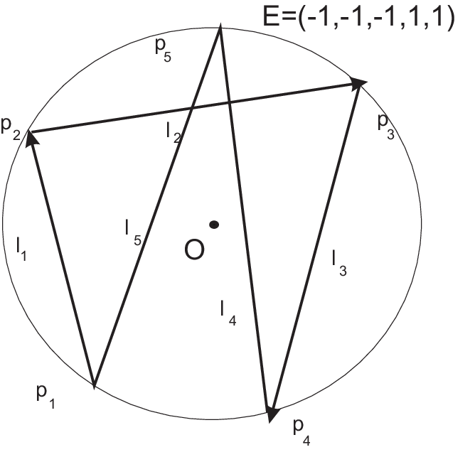
Each cyclic configuration $P$ is uniquely defined by the pair $(r_{P};E(P))$.

We start with two examples. The first one gives us the base for computation of $m(P)$. The other one is just an illustration.

Example 2.2.

[2] For a generic 4-gonal linkage, there are two possible cases:

1. The configuration space $\mathcal{M}(L)$ is disconnected. Then $L$ has four cyclic configurations listed in Fig. 3. The Morse index depends on the sign of the area $A$ and on the self-intersection of the configuration.

2. The configuration space $\mathcal{M}(L)$ is connected. Then $L$ has two cyclic configurations (the first two ones in Fig. 3).

Figure 3. 4-gonal cyclic configurations

Example 2.3.

For the equilateral pentagonal linkage $L=(1,1,1,1,1)$ there are 14 cyclic configurations listed in the Fig. 4.

(1). The convex and the anticonvex ones are the global maxima of the signed area $A$ (their Morse indices are $2$ and $0$ respectively).

(2). The starlike configurations are local maximum and a local minimum of $A$.

(3). There are $10$ more configurations that have three consecutive edges aligned. Their Morse indices equal $1$.

This can be either deduced from Theorem 4.2, or obtained by simple symmetry reasons.

Figure 4. Cyclic configurations of the equilateral pentagonal linkage and their Morse indices

3. Dynamics of Morse points. Computation of $\mathcal{H}$.

A deformation of a linkage is a one-parametric continuous family $L(t),\ t\in[0,1]$ of linkages.

In particular, we will explore cyclic deformations of a linkage $L$ which arise through the following construction.

Given a cyclic configuration $P$ of a linkage $L$, we fix the radius $r_{P}$ and force the vertices $p_{i}$ move along the circle. We get a continuous family $L(t),\ L(0)=L$ together with a continuous family of its cyclic configurations $P(t),\ P(0)=P$.

It can happen that during such a deformation, two consecutive vertices $p_{i}$ and $p_{i+1}$ meet, the edge $l_{i}$ vanishes and then appears again with a different orientation $\varepsilon_{i}$ (see Figure 5). This will be called a flip.

Given a cyclic configuration $P$, we will apply a generic cyclic deformation $P(t)$ and treat all the moments $t$ when $\mathcal{H}$ changes.

Here is a rough idea to be explored below: during a deformation $L(t)$, the Morse points move and sometimes several of them meet. By Cerf theory [1], if a Morse point meets no other Morse point, its Morse index and the value of $\mathcal{H}$ do not change. If two Morse points meet, their Morse indices satisfy $|m_{1}-m_{2}|=1$. Consequently, the values of $\mathcal{H}$ at these points are different.

Here is the precise construction:

Let $L=L(t),\ \ t\in[0,1]$ be a cyclic deformation of a generic linkage $L$.

Figure 5. A cyclic deformation passes through a flip

By generity reasons we can assume that all of $P(t)$, except for a finite number of $t$, are Morse points. Besides, we assume that no two of the following events happen at the same moment $t$.

1. $P(t)$ is a central configuration (one of the edges passes through $0$).

2. One of the edges vanishes ($t$ is the moment of a flip).

3. $\delta(P(t))=0$.

Lemma 3.1.

Assume that for some $t_{0}\in[0,1]$, the configuration $P(t_{0})$ is neither central nor has a vanishing edge. Then generically,

1. $\mathcal{H}(P(t_{0}))=0$ iff $\mathcal{H}(P(t))$ changes at $t=t_{0}$.

2. $\delta P(t_{0})=0$ iff $d(P(t))$ changes at $t=t_{0}$.

3. $\mathcal{H}(P(t))$ changes at $t=t_{0}$ if and only if $\delta P(t)$ changes its sign at $t=t_{0}$.

Sketch of the proof.

(1) and (2) follow from analysis of the formulae for $\mathcal{H}$ and $\delta P$.

Before proving (3), let us first make the following observation. Assume that a linkage $L$ and a string $E=(\varepsilon_{1},...,\varepsilon_{n})$ are fixed. There exists a cyclic configuration $P$ of $L$ with $E(P)=E$ inscribed in a circle of radius $r_{P}$ if and only if for some integer $k$, the number $r_{P}$ is a root of the function $F_{L,E}$, where

$$F_{L,E}(r)=\sum_{i=1}^{n}\varepsilon_{i}\arcsin(\frac{l_{i}}{2r})-\pi k.$$

Now prove (3).

1. Assume that $\delta P(t_{0})=0$. Then the function $F_{L,E}$ has a multiple root at $r_{P}$. Indeed, it is a root just by the above observation. Besides, we easily have

$$-\frac{dF_{L(P(t_{0})),\ E}}{dr}|_{r=r_{P}}=\sum_{i=1}^{n}\frac{\varepsilon_{i}l_{i}}{2r_{P}^{2}\sqrt{1-\sin^{2}\alpha_{i}}}=\frac{1}{2r_{P}}\sum_{i=1}^{n}\varepsilon_{i}\tan\alpha_{i}=\frac{1}{2r_{P}}\delta P(t_{0})=0$$

(Here we write for short $l_{i}$ and $\alpha_{i}$ instead of $l_{i}(P(t_{0}))$ and $\alpha_{i}(P(t_{0}))$.)

This means that the linkage $L(P(t_{0}+\varepsilon))$ has two Morse points $P(t_{0}+\varepsilon)$ and $P^{\prime}(t_{0}+\varepsilon)$ with one and the same $E(P)=E(P^{\prime})=E$ such that $P(t_{0}+\varepsilon)$ and $P^{\prime}(t_{0}+\varepsilon)$ tend to $P(t_{0})$ as $\varepsilon$ tends to zero.

By above arguments of Cerf theory and continuity reasons, $\mathcal{H}(P(t_{0}))=0$.

2. Conversely, if $\mathcal{H}(t_{0})=0$, then $P$ is a limit point of two critical points of a deformation $L(q)$. Hence $r_{P}$ is a multiple root of $F_{L,E}$.∎

Lemma 3.2.

Let a generic cyclic deformation $P(t)$ pass through a flip. Then the values of $\mathcal{H}(P)$ and $E(P)$ change, whereas the value $d(P)$ does not change.∎

Lemma 3.3.

If during a generic cyclic deformation $P(t)$ passes a central configuration, then $d(P)$ and $E(P)$ change, but $\mathcal{H}(P)$ remains constant.∎

Taken together, the three lemmata imply the first main result of the paper:

Theorem 3.4.

Let $P$ be a generic cyclic configuration.

Denote by $e(P)$ the number of positive entries in $E(P)=(\varepsilon_{1},...,\varepsilon_{n})$.

Remind that $d(P)$ the sign of $\delta(P)$. Then

$$\mathcal{H}(P)=-d(P)(-1)^{e(P)}$$

Proof. Consider a generic cyclic deformation joining $P$ and some convex cyclic configuration $P_{CONV}$ with the same number of vertices.

For $P_{CONV}$ the theorem is obviously valid. Besides, the above three lemmata imply that the product $\mathcal{H}(P(t))\cdot d(P(t))(-1)^{e(P(t))}$ does not change as $t$ changes. ∎

4. Computation of the Morse index

The following lemma provides an inductive computation of $m(P)$.

Lemma 4.1.

Let $P$ be a generic cyclic configuration. Adding its diagonal $p_{i}p_{j}$, we express $P$ as the homological sum of a cyclic configurations $P_{1}$ and a trigonal cyclic configuration $P_{2}$ (see Fig. 6). Then

1. Either $m(P)=m(P_{1})$ or $m(P)=m(P_{1})+1.$

2. The Morse index $m(P_{1})$ together with $\mathcal{H}(P)$ uniquely determine $m(P)$.

Sketch of the proof:

(1) follows from the fact that the moduli space $\mathcal{M}(P_{1})$ is a codimension one submanifold of $\mathcal{M}(P)$; (2) easily follows from (1).∎

Figure 6. Homological decomposition $P=P_{1}+P_{2}$

Iterative application of the above lemma starting from 4-gonal linkages immediately implies the final theorem:

Theorem 4.2.

Let $P=(p_{1},...,p_{n})$ be a generic cyclic configuration. Introduce its subconfigurations $P_{3},...,P_{n}$ (see Fig. 7)

$$P_{i}=(p_{1},...,p_{i}),\ \ i=3,...,n.$$

Put $\mathcal{H}(P_{3})=1$ for the trigonal configuration $P_{3}$.

Then the Morse index $m(P)$ equals the number of the sign changes in the sequence

$$\mathcal{H}(P_{3}),\mathcal{H}(P_{4}),\mathcal{H}(P_{5}),...,\mathcal{H}(P_{n}),$$

where the values $\mathcal{H}(P_{i})$ are already known by Theorem 3.4. ∎

Figure 7. Subconfigurations of $P$

References

- [1] J.Cerf, La stratification naturelle des espaces de fonctions differentiables reelles et le theoreme de la pseudo-isotopie, Inst. Hautes Et. Sci. Publ. Math. No. 39 (1970), 5-173.
- [2] E.Elerdashvili, M.Jibladze, G.Khimshiashvili, Cyclic configurations of pentagon linkages, Bull. Georgian Nat. Acad. Sci. 2 (2008), No.4, 13-16.
- [3] M.Farber, D.Schütz, Homology of planar polygon spaces, Geom. Dedicata 125 (2007),75-92.
- [4] C.Gibson, P.Newstead, On the geometry of the planar 4-bar mechanism, Acta Applic. Math. 7 (1986), 113-135.
- [5] G.Khimshiashvili, On configuration spaces of planar pentagons, Zap. Nauch. Sem. S.-Peterb. Otdel. Mat. Inst. RAN 292(2002), 120-129.
- [6] G.Khimshiashvili, Signature formulae and configuration spaces, J. Math. Sci. (accepted).
- [7] G.Khimshiashvili, G. Panina, Cyclic polygons are critical points of area. Zap. Nauchn. Semin. POMI 360 (2008), 238–245.
- [8] D.Robbins, Areas of polygons inscribed in a circle, Discrete Comput. Geom. 12(1994), 223-236.