Tree polymers in the infinite volume limit at
critical strong disorder

Abstract

The a.s. existence of a polymer probability in the infinite volume limit is readily obtained under general conditions of weak disorder from standard theory on multiplicative cascades or branching random walk. However, speculations in the case of strong disorder have been mixed. In this note existence of an infinite volume probability is established at critical strong disorder for which one has convergence in probability. Some calculations in support of a specific formula for the a.s. asymptotic variance of the polymer path under strong disorder are also provided.

Torrey Johnson and Edward C Waymire

[Oregon State University]Torrey Johnson Department of Mathematics, Oregon State Univeristy, Corvallis, Oregon 97331 johnsotor@science.oregonstate.edu [Oregon State Univeristy]Edward C Waymire Department of Mathematics, Oregon State Univeristy, Corvallis, Oregon 97331 waymire@math.oregonstate.edu

60K3560G42;82D30

1 Introduction and Preliminaries

Polymers are abstractions of chains of molecules embedded in a solvent by non-self-intersecting polygonal paths of points whose probabilities are themselves random (reflecting impurities of the solvent). In this connection, tree polymers take advantage of a particular way to determine path structure and their probabilities as follows.

Three different references to paths occur in this formulation. An $\infty$-tree path is a sequence $s=(s_{1},s_{2},\ldots)\in\{-1,1\}^{\mathbb{N}}$ emanating from a root $0$. A finite tree path or vertex $v$ is a finite sequence $v=s|n=(s_{1},\ldots,s_{n})$, read “path $s$ restricted to level $n$”, of length $|v|=n$. The symbol $*$ denotes concatenation of finite tree paths; if $v=(v_{1},\ldots,v_{n})$ and $t=(t_{1},\ldots,t_{m})$, then $v*t=(v_{1},\ldots,v_{n},t_{1},\ldots,t_{m})$. Vertices belong to $T:=\bigcup_{n=0}^{\infty}\{-1,1\}^{n}$, and can be viewed as unique finite paths to the root of the directed binary tree $T$ equipped with the obvious graph structure. We also write

$$\partial T=\{-1,1\}^{\mathbb{N}}$$

for the boundary of $T$. The third type of path, and the one of main interest to polymer questions, is that of the polygonal tree path defined by $n\rightarrow(s)_{n}:=\sum_{j=1}^{n}s_{j}$, $n\geq 0$, with $(s)_{0}:=0$, for a given $s\in\partial T$.

$\partial T$ is a compact, topological Abelian group for coordinate-wise multiplication and the product topology. The uniform distribution on $\infty$-tree paths is the Haar measure on $(\partial T,\mathcal{B})$, i.e.

$$\lambda(ds)=\left(\frac{1}{2}\delta_{+}(ds)+\frac{1}{2}\delta_{-}(ds)\right)^{\mathbb{N}}.$$

Let $\{X_{v}:v\in T\}$ be an i.i.d. family of positive random variables on $(\Omega,\mathcal{F},P)$ with $\mathbb{E}X<\infty$; we denote a generic random variable with the common distribution of $X_{v}$ by $X$. Without loss of generality we may assume that $\mathbb{E}X=1$. Define a sequence of random probability measures $\text{prob}_{n}(ds)$ on $(\partial T,\mathcal{B})$ by the prescription that

$$\text{prob}_{n}(ds)<<\lambda(ds)$$

with

$$\frac{d\text{prob}_{n}}{d\lambda}(s)=Z_{n}^{-1}\prod_{j=1}^{n}X_{s|j}$$

where

$$Z_{n}=\int_{\partial T}\prod_{j=1}^{n}X_{s|j}\lambda(ds)=\sum_{|s|=n}\prod_{j=1}^{n}X_{s|j}2^{-n}.$$

Observing that $\{Z_{n}:n=1,2\ldots\}$ is a positive martingale, it follows that

$$Z_{\infty}:=\lim_{n\rightarrow\infty}Z_{n}$$

exists a.s. in $(\Omega,\mathcal{F},P)$. According to a classic theorem of Kahane and Peyrière (1976) in the context of multiplicative cascades, and Biggins (1976) in the context of branching random walks, one has the following dichotomy:

$$P(Z_{\infty}>0)=1\quad \Longleftrightarrow\quad\mathbb{E}X\ln X<\ln 2$$

$$P(Z_{\infty}=0)=1\quad \Longleftrightarrow\quad\mathbb{E}X\ln X\geq\ln 2.$$

The a.s. occurance of the event $[Z_{\infty}>0]$ is refered to as weak disorder and that of $[Z_{\infty}=0]$ as strong disorder; see Bolthausen (1989). In particular, the critical case $\mathbb{E}X\ln X=\ln 2$ is strong disorder. In the case of tree polymers one may view the notions of weak/strong in terms of a disorder parameter defined by $\mathbb{E}X\ln X$ and relative to the branching rate, $\ln 2$.

In this short communication we provide some new insights into a few delicate problems for the case of strong disorder.

2 Tree Polymers under Weak Disorder

To set the stage for contrast, we record a rather robust consequence of weak disorder.

Theorem 2.1.

Under weak disorder, there is a random probability measure $\text{\emph{prob}}_{\infty}(ds)$ on $(\partial T,\mathcal{B})$ such that a.s.

$$\text{\emph{prob}}_{n}(ds)\Rightarrow\text{\emph{prob}}_{\infty}(ds)$$

where $\Rightarrow$ denotes weak convergence.

Proof 2.2.

Define $\lambda_{n}(ds)=Z_{n}\text{prob}_{n}(ds)$, $n=1,2,\ldots$. By Kahane’s $T$-martingale theory, e.g., Kahane (1989), $\lambda_{n}(ds)$ converges vaguely to a non-zero random measure $\lambda_{\infty}(ds)$ on $(\partial T,\mathcal{B})$ with probability one. By definition of weak disorder $Z_{n}\rightarrow Z_{\infty}>0$ a.s., thus we obtain

$$\text{prob}_{n}(ds)=Z_{n}^{-1}\lambda(ds)\Rightarrow Z_{\infty}^{-1}\lambda_{\infty}(ds)\quad\text{a.s.}$$

Notice that in the case of no disorder, i.e. $X=1$ a.s., one has

$$\text{prob}_{n}(ds)=\lambda(ds)\quad\forall n=1,2,\ldots.$$

Moreover, under $\lambda(ds)$, the polygonal paths are simply symmetric simple random walk paths, where the probability theory is quite will-known and complete. For example, the central limit theorem takes the form

$$\lim_{n\rightarrow\infty}\lambda\left(\left\{s\in\partial T:\frac{(s)_{n}}{\sqrt{n}}\leq x\right\}\right)=\frac{1}{\sqrt{2\pi}}\int_{-\infty}^{x}e^{-\xi^{2}/2}d\xi.$$

For probability laws involving convergence in distribution, one may ask if the CLT continues to hold a.s. with $\lambda(ds)$ replaced by $\text{prob}_{n}(ds)$. This form of universality was answered in the affirmative by Waymire and Williams (2010) for weak disorder under the additional assumption that $\mathbb{E}X^{1+\delta}<\infty$ for some $\delta>0$. Problems involving limit laws such as a.s. strong laws, a.s. laws of the iterated logarithm, etc, however, require an infinite volume probability $\text{prob}_{\infty}(ds)$ for their formulation. While the preceding proposition answers this in the case of weak disorder, the problem is open for strong disorder. Moreover, it has been speculated by Yuval Peres (private communication) that $\text{prob}_{n}(ds)$ will a.s. have infinitely many weak limit points under strong disorder. However, in the case of critical strong disorder we show that a natural infinite volume polymer exists and is related to the finite volume polymers through limits in probability.

3 Tree Polymers at Critical Strong Disorder

In this section we show the existence under critical strong disorder, i.e., assuming $\mathbb{E}X\ln X=\ln 2$, of an infinite volume polymer probability $\text{prob}_{\infty}(ds)$ that may be viewed as the weak limit in probability of the sequence $\text{prob}_{n}(ds),n\geq 1,$ in the sense that its characteristic function is the limit in probability of the corresponding sequence of characteristic functions of $\text{prob}_{n}(ds),n\geq 1$.

For $v\in T$, $v=(v_{1},\ldots,v_{m})$, say, let

$$\Delta_{m}(v)=\{s\in\partial T:s_{i}=v_{i},\text{ }i=1,\ldots,m\},\qquad|v|=m.$$

Since $T$ is countable there are countably many such finite-dimensional rectangles in $\partial T$.

For $m>n$, note that

$$\text{prob}_{n}(\Delta_{m}(v)) =\int_{\Delta_{m}(v)}\frac{d\text{prob}_{n}}{d\lambda}(s)\lambda(ds)$$

$$=\int_{\Delta_{m}(v)}Z_{n}^{-1}\prod_{j=1}^{n}X_{s|j}\lambda(ds)$$

$$=Z_{n}^{-1}\int_{\Delta_{m}(v)}\prod_{j=1}^{n}X_{v|j}\lambda(ds)$$

$$=Z_{n}^{-1}\prod_{j=1}^{n}X_{v|j}\cdot 2^{-m}.$$

For example,

$$\text{prob}_{1}(\Delta_{m}(v)) =Z_{1}^{-1}X_{v|1}2^{-m},\qquad Z_{1}=\frac{X_{+}+X_{-}}{2}$$

$$=\frac{X_{v|1}2^{-(m-1)}}{X_{+}+X_{-}}$$

$$=\left\{\begin{array}[]{rl}\frac{X_{+}2^{-(m-1)}}{X_{+}+X_{-}},&\quad v|1=+1\\ \frac{X_{-}2^{-(m-1)}}{X_{+}+X_{-}},&\quad v|1=-1.\end{array}\right.$$

$\sum_{|v|=m}\text{prob}_{1}(\Delta_{m}(v))=1$ since there are $2^{m}$ such $v$’s, half of which have $v_{1}=+1$ and the other half have $v_{1}=-1$.

For $m\leq n,|v|=m$, we have

$$\text{prob}_{n}(\Delta_{m}(v)) =Z_{n}^{-1}\int_{\Delta_{m}(v)}\prod_{j=1}^{n}X_{s|j}\lambda(ds)$$

$$=Z_{n}^{-1}\prod_{j=1}^{m}X_{v|j}\sum_{|t|=n-m}\prod_{j=1}^{n-m}X_{(v*t)|j}2^{-n}$$

$$=Z_{n}^{-1}\left(\prod_{j=1}^{m}X_{v|j}2^{-m}\right)Z_{n-m}(v),$$

where

$$Z_{0}(v)=1,\quad Z_{n-m}(v)=\sum_{|t|=n-m}\prod_{j=1}^{n-m}X_{(v*t)|j}2^{-(n-m)}.$$

In particular, $Z_{n}=Z_{n}(0)$, where $0\in T$ is the root.

Note that

$$Z_{n} =\sum_{|u|=m}\sum_{|t|=n-m}\prod_{j=1}^{m}X_{u|j}2^{-m}\prod_{j=1}^{n-m}X_{(u*t)|j}2^{-(n-m)}$$

$$=\sum_{|u|=m}Z_{n-m}(u)\prod_{j=1}^{m}X_{u|j}2^{-m}.$$

Thus, letting $a_{k}=1/\sqrt{k},k\geq 1$,

$$\text{prob}_{n}(\Delta_{m}(v)) =\frac{D_{n-m}(v)\prod_{j=1}^{m}X_{v|j}2^{-m}\frac{Z_{n-m}(v)}{a_{n-m}D_{n-m}(v)}}{\sum_{|u|=m}D_{n-m}(u)\left(\prod_{j=1}^{m}X_{v|j}2^{-m}\right)\frac{Z_{n-m}(u)}{a_{n-m}D_{n-m}(u)}}$$

$$\longrightarrow\frac{D_{\infty}(v)\prod_{j=1}^{m}X_{v|j}2^{-m}}{\sum_{|u|=m}D_{\infty}(u)\left(\prod_{j=1}^{m}X_{v|j}2^{-m}\right)}$$

where (i) the convergence to $D_{\infty}(v)$ is the almost sure limit of the derivative martingale obtained by Biggins and Kyprianou (2004), and (ii) $\lim_{n\rightarrow\infty}\frac{Z_{n-m}(v)}{a_{n-m}D_{n-m}(v)}=c>0$ is the limit in probability at critical strong disorder recently obtained by Aidékon and Shi (2011). The constant $c=({2\over\pi\sigma^{2}})^{1/2}$, for $\sigma^{2}=\mathbb{E}\{X(\ln(X))^{2}\}-(\mathbb{E}\{X\ln(X)\})^{2}>0$, does not depend on $v\in T$. Aidékon and Shi (2011) also point out that the almost sure positivity of $D_{\infty}(v)$ follows from Biggins and Kyprianou (2004) and Aidékon (2011) The sequence $a_{k}=k^{-{1\over 2}},k\geq 1,$ is referred to as the Seneta-Heyde scaling.

Remark 3.1.

For each $v\in T$, there is a set $N(v)$ of probability zero such that

$$D_{\infty}(v,\omega)=\lim_{n\rightarrow\infty}D_{n}(v,\omega),\quad\omega\in\Omega\backslash N(v).$$

Since $T$ is countable, the set $N=\bigcup_{v\in T}N(v)$ is still a $P$-null subset of $\Omega$. The almost sure convergence of the derivative martingales is essential to the construction of $\text{\emph{prob}}_{\infty}$ given in the lemma below.

We now define

$$\text{prob}_{\infty}(\Delta_{m}(v),\omega)=\frac{D_{\infty}(v,\omega)\prod_{j=1}^{m}X_{v|j}(\omega)2^{-m}}{\sum_{|u|=m}D_{\infty}(u,\omega)\left(\prod_{j=1}^{m}X_{u|j}(\omega)2^{-m}\right)}$$

for $\omega\in\Omega\backslash N$.

Lemma 3.2.

$\text{\emph{prob}}_{\infty}(\Delta_{m}(v),\omega)$ extends to a unique probability on $(\partial T,\mathcal{B})$ for each $\omega\in\Omega\backslash N$.

Proof 3.3.

We use Caratheodory extension, taking careful advantage of the fact that the sets $\Delta(v)$, $v\in T$, are both open and closed subsets of the compact set $\partial T$. For $\omega\in\Omega\backslash N$, $\text{prob}_{\infty}(\cdot,\omega)$ extends to the algebra generated by $\{\Delta(v):v\in T\}$ by addition. Since $\partial T$ is compact and the rectangles are both open and closed, countable additivity on this algebra must hold as a consequence of finite additivity; i.e. if $\bigcup_{i=1}^{\infty}\Delta(v_{i})$ is contained in the algebra generated by $\{\Delta(v):v\in T\}$, then $\bigcup_{i=1}^{\infty}\Delta(v_{i})$ is closed, hence compact, and its own open cover, i.e. $\bigcup_{i=1}^{\infty}\Delta(v_{i})=\bigcup_{i=1}^{l}\Delta(v_{i_{l}})$ for some finite subsequence $\{i_{j}\}_{j=1}^{l}$ of $\{1,2,\ldots\}$.

Theorem 3.4.

At critical strong disorder, for each finite set $F\subseteq\mathbb{N}$

$$\widehat{\text{\emph{prob}}_{n}(F)}\quad\Rightarrow\quad\widehat{\text{\emph{prob}}_{\infty}(F)}\qquad\text{in probability},$$

where $\widehat{\text{\emph{prob}}}_{n},n\geq 1,\widehat{\text{\emph{prob}}}_{\infty}$ denote their respective Fourier transforms as probabilities on the compact abelian multiplicative group $\partial T$ for the product topology.

Proof 3.5.

The continuous characters of the group $\partial T$ are given by

$$\chi_{F}(t)=\prod_{j\in F}t_{j}\quad\text{for finite sets }F\subseteq\mathbb{N}.$$

In particular there are only countably many characters of $\partial T$. From standard Fourier analysis it follows that we need only show that

$$\lim_{n\rightarrow\infty}\mathbb{E}_{\text{prob}_{n}}\chi_{F}=\mathbb{E}_{\text{prob}_{\infty}}\chi_{F}\quad\text{in probability}$$

for each finite set $F\subseteq\mathbb{N}$. Let $m=\text{max}\{k:k\in F\}$. Then for $n>m$,

$$\mathbb{E}_{\text{prob}_{n}}\chi_{F} =\int_{\partial T=\bigcupdot_{|v|=m}\Delta_{m}(v)}\chi_{F}(s)\frac{d\text{prob}_{n}}{d\lambda}(s)\lambda(ds)$$

$$=\sum_{|v|=m}\left(\prod_{j\in F}v_{j}\right)Z_{n}^{-1}(0)\prod_{j=1}^{m}X_{v|j}2^{-m}\sum_{|t|=n-m}\prod_{j=1}^{n-m}X_{(v*t)|j}2^{-(n-m)}$$

$$=\sum_{|v|=m}\left(\prod_{j\in F}v_{j}\right)\prod_{j=1}^{m}X_{v|j}2^{-m}\frac{Z_{n-m}(v)}{Z_{n}(0)}$$

$$=\sum_{|v|=m}\left(\prod_{j\in F}v_{j}\right)\prod_{j=1}^{m}X_{v|j}2^{-m}D_{n-m}(v)\frac{\frac{Z_{n-m}(v)}{a_{n-m}D_{n-m}(v)}}{\sum_{|u|=m}\prod_{j=1}^{m}X_{u|j}2^{-m}D_{n-m}(u)\frac{Z_{n-m}(u)}{a_{n-m}D_{n-m}(u)}}$$

$$\longrightarrow\mathbb{E}_{\text{prob}_{\infty}}\chi_{F},$$

where the convergence is almost sure for terms of the form $D_{n-m}$ and in probability for those of the form $Z_{n-m}/(a_{n-m}D_{n-m})$ as $n\to\infty$.

4 Diffusivity Problems at Strong Disorder

With regard to the aforementioned a.s. limits in distribution of polygonal tree paths, Waymire and Williams (2010) also obtained a.s. limits of the form

$$\lim_{n\to\infty}{\ln E_{prob_{n}}e^{r(S)_{n}}\over n}=F(r)$$

under both weak and strong disorder. Let us refer to these as almost sure Laplace rates in reference to the Laplace principle of large deviation theory.

In the case of weak disorder the universal limit is $F(r)=\ln\cosh(r)$, in a neighborhood of the origin, otherwise independent of the distribution of $X$. In addition to being independent of the distribution of $X$ within the range of weak disorder, this universality of Laplace rates is manifested in the coincidence with the same limit obtained for $X\equiv 1$, i.e., for simple symmetric random walk.

For an illustrative case of strong disorder, consider $X=e^{\beta Z-{\beta^{2}\over 2}}$, where $Z$ is standard normal and $\beta\geq\beta_{c}=\sqrt{2\ln 2}$. Then from Waymire and Williams (2010), it follows that a.s. in a neighborhood of the origin that

$$F(r)=r\tanh(rh(r))+\beta^{2}h(r)-\beta\beta_{c},$$

where $h(r)$ is the uniquely determined solution to

$$\beta^{2}h^{2}(r)+2rh(r)\tanh(rh(r))-2\ln\cosh(rh(r))=\beta_{c}^{2};$$

also see Waymire and Williams (Sec 6, Cor 2, 2010) for the general formulae in the case of strong disorder. In particular, the universality of the Laplace rates breaks down, even at critical strong disorder. A graph of $F(r)$ computed from MATLAB is indicated in Figure 1 for the strong disorder case of $\beta=2\beta_{c}$.

Figure 1: Graph of the function $F$ for various $\beta$.

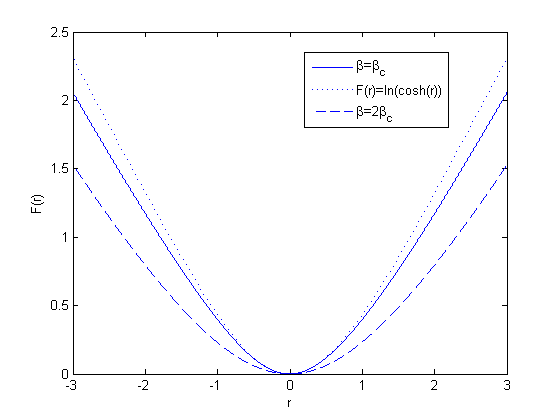
Using the equations defining $F(r)$ one may easily verify that $F(0)=0,F^{\prime}(0)=0$ and $F^{\prime\prime}(0)={2\beta\beta_{c}-\beta_{c}^{2}\over\beta^{2}}$. While these specific calculations follow directly from the general results of Waymire and Williams (2010), from here one is naturally lead to speculate that the asymptotic variance under strong disorder is obtained under diffusive scaling by $\sqrt{n}$ precisely as

$$\sigma^{2}(\beta)={2\beta\beta_{c}-\beta_{c}^{2}\over\beta^{2}},\quad\beta\geq\beta_{c}.$$

In particular this formula continuously extends the weak disorder variance $\sigma^{2}(\beta)\equiv 1,\beta<\beta_{c},$ across $\beta=\beta_{c}$. In any case, this quantity is a basic parameter of the rigorously proven limit $F(r)$.

5 Acknowledgment

The authors thank the referee for spotting a serious error in the original draft and providing the reference to Aidékon and Shi (2011) used in this paper. The first author was partially supported by an NSF-IGERT-0333257 graduate training grant in ecosystems informatics at Oregon State University, and the second author was partially supported by a grant DMS-1031251 from the National Science Foundation.

References

- [1] Aidékon, E.(2011). Convergence in law of a minimum of a branching random walk, arXiv: 1101.1810.
- [2] Aidékon, E., Z. Shi (2011). Martingale ratio convergence in the branching random walk, arXiv:1102.0217
- [3] Bezerra, S., Tindel, S. and Viens, F. (2008). Superdiffusivity for a Brownian polymer in a continuous Gaussian environment. \AP 36(5), 1642–1675.
- [4] Biggins, J.D. (1976). The first-and-last-birth problem for a multitype age-dependent branching process. \AAP 8, 446–459.
- [5] Biggins, J.D. and Kyprianou, A.E. (2004). Measure change in multitype branching, \AP 36, 544–581.
- [6] Bolthausen, E. (1989). A note on diffusion of directed polymers in a random environment. \CMP 123, 529–534.
- [7] Bolthausen, E. (1991). On directed polymers in a random environment. Selected Proceedings of the Sheffield Symposium on Applied Probability, eds. I.V. Basawa, R.I. Taylor, IMS Lecture Notes Monograph Series. 18, 41–47.
- [8] Comets, F. and Yoshida, N. (2006). Directed polymers in random environment are diffusive at weak disorder. \AP 34(5), 1746–1770.
- [9] Hu, Y. and Shi, Z. (2009). Minimal position and critical martingale convergence in branching random walks, and directed polymers on disordered trees. \AP 37(2), 742–789.
- [10] Kahane, J-P. (1989). Random multiplications, random coverings, and multiplicative chaos. Proceedings of the Special Year in Modern Analysis, E. Berkson, N. Tenney Peck, J. Jerry Uhl, eds., London Math. Soc. Lect. Notes, Cambridge Univ. Press, London. 137, 196–255.
- [11] Kahane, J-P. and Peyrière, J. (1976). Sur certaines martingales de Benoit Mandelbrot. Adv. in Math. 22, 131–145.
- [12] Waymire, E. and Williams, S.C. (1994). A general decomposition theory for random cascades. \BAMS 31(2), 216–222.
- [13] Waymire, E. and Williams, S.C. (1995). Multiplicative cascades: dimension spectra and dependence. J. Four. Anal. and Appl., special issue to honor J-P. Kahane, 589–609.
- [14] Waymire, E. and Williams, S.C. (1996). A cascade decomposition theory with applications to Markov and exchangeable cascades. \TAMS 348(2), 585–632.
- [15] Waymire, E. and Williams, S.C. (1995). Markov cascades. IMA Volume on Branching Processes, eds., K. Athreya and P. Jagers, Springer-Verlag, NY.
- [16] Waymire, E. and Williams, S.C. (2010). T-martingales, size-biasing and tree polymer cascades. Fractals and Related Fields, ed., J. Barral. http://www.math.oregonstate.edu/~waymire/index.html (to appear).