Entangling capacity with local ancilla

Abstract

We investigate the entangling capacity of a dynamical operation with access to local ancilla. A comparison is made between the entangling capacity with and without the assistance of prior entanglement. An analytic solution is found for the log-negativity entangling capacity of two-qubit gates, which equals the entanglement of the Choi matrix isomorphic to the unitary operator. Surprisingly, the availability of prior entanglement does not affect this result; a property we call resource independence of the entangling capacity. We prove several useful upper-bounds on the entangling capacity that hold for general qudit dynamical operations, and for a whole family of entanglement measures including log-negativity and log-robustness. The log-robustness entangling capacity is shown to be resource independent for general dynamics. We provide numerical results supporting a conjecture that the log-negativity entangling capacity is resource independence for all two-qudit unitaries.

Quantum information theory, and its various practical applications, has lead to a mature theory of entanglement as a resource. It is now common to think of entanglement as almost a fungible commodity. Two different quantum states with manifestly very different non-locality properties may sometimes be converted into each other by local operations, they can also be be diluted [1] and distilled [2]. The laws governing the capabilities of local operations to interchange between different entangled states are understood in terms of entanglement measures and monotones that quantify the amount of entanglement in a given quantum state [3].

Entanglement can be created in physical systems where there is a suitable non-local dynamical process. As we can quantify the entanglement of quantum states, we can quantify the efficacy of a dynamical operation at producing entanglement. Such quantities are called the entangling power, capacity or strength [4] of a dynamical process. The average entanglement generated by unitaries, commonly called the entangling power, has been studied by Zanadri and coworkers [5, 6, 7]. Whereas the maximum entanglement that can be produced by two-qubit unitaries is usually called the entangling capacity [8, 9, 10]. In the practical context of attempting to maximize entanglement production for utilization as part of a quantum information protocol, the most appropriate quantity is the entanglement capacity (EC).

Kraus and Cirac consider the EC for two-qubit unitaries acting on two-qubit product states [8]. Leifer et al extended this analysis to find the entangling capacity when the initial two-qubit state has prior entanglement [9], and found that this can boost the entangling capacity. In both papers it was observed that access to local ancilla can enable much higher entangling capacities for some unitaries, with the swap gate as the most striking example. Without local ancilla the swap gate has zero entangling capacity, but with local ancilla the swap gate can produce two Bell pairs. Despite numerous examples where local ancilla prove beneficial, no previous work has established an analytic solution for the entangling capacity with access to local ancilla.

Figure 1: The maximum increase in entanglement created by a phase gate, $U=\exp^{i\phi Z_{A}Z_{B}}$, as measured by: (thick blue) the von Neumann entropy with initially separable states; (thin blue) the von Neumann entropy without prior entanglement; (thick purple) the log-negativity both with and without access to prior entanglement.

We prove that two qubit unitaries have an EC, measured by the log-negativity [11, 12], that has a simple closed form. Interestingly this EC equals the entanglement of the Choi matrix $\rho_{U}$ isomorphic to $U$ via the Choi-Jamiolkowski isomorphism [13, 14]. Cirac et al [15] have previously proposed quantifying entangling power by considering the entanglement of the Choi matrix. However, Cirac et al did not show that the Choi matrix captures the maximum achievable entanglement for any continuous monotones. Our results give a concrete operational meaning to the entanglement of the Choi matrix.

It is surprisingly that our result for two-qubit unitaries holds with or without the assistance of prior entanglement. We call this property resource-independence of the log-negativity EC for two-qubits. In deriving our result for two-qubit unitaries, we prove two theorems that are useful in their own right. These theorems provide upper-bounds on the EC in the more general setting of two-qudit completely positive trace preserving maps. The first upper-bound we prove also applies to a whole family of EC monotones that includes both log-negativity EC and log-robustness EC. Our upper-bounds entail that log-robustness EC is always resource independent, and give us reason to suspect that log-negativity is always resource-independent. We support this conjecture with a numerical study of the log-negativity EC for two-qutrit unitaries, where we found no violations of resource-independence.

I Notation and Definitions

We are interested in solving the following problem: for a given completely-positive trace-preserving (CPTP) map $\Lambda$ acting on Hilbert spaces $H_{a}\otimes H_{b}$, what is the maximum entanglement that can be produced? This maximization problem depends on what resources are available. Throughout, we assume that local ancilla, local unitaries and classical communication are freely available as is appropriate in many communication and distributed computation scenarios. The maximum achievable entanglement for a dynamical map, $\Lambda$, when the initial state is separable, is given by:

$$E(\Lambda)=\sup\{E(\Lambda(\sigma))|\sigma\in\mathcal{S}\},$$ (1)

where $\mathcal{S}$ denotes the set of separable density matrices, and $E(\rho)$ is an appropriate entanglement monotone for density matrices. However, when prior entanglement is available, the maximum increase in entanglement is:

$$E^{\mathcal{D}}(\Lambda)=\sup\{E(\Lambda(\sigma))-E(\sigma)|\sigma\in\mathcal{D}\},$$ (2)

where $\mathcal{D}$ is the set of all physical density matrices, and we have denoted the availability of this resource by a superscript. This quantity cannot be smaller than the unassisted power, $E(\Lambda)$, but in general may be larger. The von Neumann entropy, $E_{vN}$, is an example where some unitary gates have been shown to exhibit an increase, $E_{vN}^{\mathcal{D}}(U)>E_{vN}(U)$, when assisted by entanglement [16]. We do not need to invoke exotic unitary gates to observe the phenomena, as it occurs even for simple two-qubit phase gates, as shown in Fig. 1. Alternatively, we may be interested in knowing how much entanglement could be produced given access to a restricted class of resources, such as bound entanglement [17]:

$$E^{\mathcal{B}}(\Lambda)=\sup\{E(\Lambda(\sigma))-E(\sigma)|\sigma\in\mathcal{B}\},$$ (3)

where $\mathcal{B}$ is the set of all physical density matrices with only bound entanglement. Formally, all operators in $\mathcal{B}$ are positive semi-definite before and after partial transposition.

Since the von Neumann EC violates resource-independence, such that $E_{vN}^{\mathcal{D}}\neq E_{vN}$, there is a temptation to infer that this phenomena would be observed for other EC monotones. Here we present results that counter this intuition, showing that many other entanglement monotones have an inherent resource independence, which makes them cleaner, and simpler, candidates for EC monotones.

We are principally interested in the logarithmic versions of negativity [11, 12] and robustness [18] and other similar decomposition-based monotones (defined in section II.). The negativity is defined as:

$$E_{N}(\rho)=(||\rho^{\Gamma}||-1)/2$$ (4)

where $\Gamma$ denotes a partial transpose over system $B$, and $||...||$ denotes the trace norm:

$$||A||=\mathrm{tr}\left(\sqrt{A^{\dagger}A}\right).$$ (5)

The robustness of $\rho$ was first defined [18] as the amount of any separable state $\sigma^{\prime}$ that must be mixed with $\rho$ to make the whole mixture separable:

$$E_{S}(\rho)=\inf\{t|\sigma=\frac{\rho+t\sigma^{\prime}}{1+t};\sigma,\sigma^{\prime}\in\mathcal{S}\},$$ (6)

where $\mathcal{S}$ is again the set of separable states. Despite the contrast between the conventional definitions of $E_{N}$ and $E_{S}$, we will see that they are actually very closely related [11]. Throughout, we are interested in the logarithmic variant of both monotones as $E_{Lx}(\rho)=\log_{2}(1+2E_{x}(\rho))$.

Our particular interest in log-negativity is warranted as it is strongly additive:

$$E_{LN}(\rho_{1}\otimes\rho_{2})=E_{LN}(\rho_{1})+E_{LN}(\rho_{2}),$$ (7)

which is an extremely useful and intuitive property of an entanglement monotone. Any EC monotone that is both resource-independent and strongly additive has the following elegant property: given a dynamical map $\Lambda$ with entangling power $E(\Lambda)$, we can use the dynamical map $n$ times to produce, at best, exactly $nE(\Lambda)$ entanglement. Furthermore, the log-negativity provides an upperbound on the number of singlets that can be distilled [19].

Note that, our notation for EC monotones always uses a calligraphic superscript to denote the resources that are relevant to the maximization problem, and a subscript to describe the underlying entanglement monotone for quantum states.

II Decomposition-based monotones

Figure 2: An heuristic diagram of the space of matrices that are Hermitian and unit-trace, with important subsets shown. The subsets satisfy the following additional constraints: operators in $\mathcal{D}$ have non-negative eigenvalues; operators in $\mathcal{N}$ have partial transposes with non-negative eigenvalues; operators in $\mathcal{P}$ have both the previous properties; operators in $\mathcal{S}$ can be decomposed as a positive sum of separable operators.

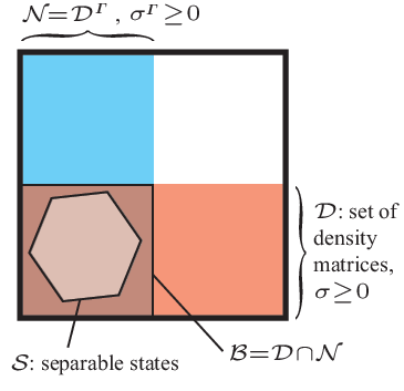
Here we introduce the idea of decomposition-based monotones of entanglement, as first discovered by Werner and Vidal [11]. They proposed entanglement monotones of the form:

$$E_{\mathcal{M}}(\rho)=\inf\{t|\rho=(1+t)\sigma^{+}-t\sigma^{-};t\geq 0;\sigma^{\pm}\in\mathcal{M}\},$$ (8)

with the minimization performed over all real linear decompositions of $\rho$ into matrices $\sigma^{\pm}$ that belong to a set $\mathcal{M}$, with the following properties :

1. the set $\mathcal{M}$ is a compact and convex, such that $p\sigma+(1-p)\sigma^{\prime}\in\mathcal{M}$, whenever $\sigma,\sigma^{\prime}\in\mathcal{M}$ and $0\leq p\leq 1$;

2. all matrices in $\mathcal{M}$ are Hermitian and unit-trace, so $\sigma=\sigma^{\dagger}$ and $\mathrm{tr}(\sigma)=1$;

3. the set $\mathcal{M}$ includes all separable states, $\mathcal{S}\subseteq\mathcal{M}$;

4. the set is invariant under local unitaries, $(U_{A}\otimes U_{B})\mathcal{M}(U_{A}\otimes U_{B})^{\dagger}=\mathcal{M}$.

For any appropriate set, $\mathcal{M}$, and any Hermitian unit-trace matrix $\rho$ we can always find a decomposition $\rho=(1+t)\sigma^{+}-t\sigma^{-}$. That is, the real-linear hull of the set $\mathcal{M}$ spans the space of Hermitian unit-trace operators. This result is well known for the set of separable states [18], $\mathcal{S}$, and so will also hold for any set that contains $\mathcal{S}$. These properties ensure that $E_{\mathcal{M}}$ is always an entanglement monotone, and similarly  for logarithmic quantities, which we denote:

$$E_{L\mathcal{M}}(\rho)=\log_{2}(1+2E_{\mathcal{M}}(\rho)).$$ (9)

Familiar monotones in this family include negativity and robustness of entanglement, which are:

$$E_{S}(\rho) = E_{\mathcal{S}}(\rho),$$

$$E_{N}(\rho) = E_{\mathcal{N}}(\rho),$$

where $\mathcal{S}$ is the set of separable matrices, and $\mathcal{N}=\mathcal{D}^{\Gamma}$. The equivalence for robustness is immediate, but for negativity requires a little work [11]. For an overview of how these sets relate see figure. 2. In addition to more familiar entanglement monotones, Vidal and Werner also discussed an intermediate monotone for the set $\mathcal{B}$ that contains $\sigma$ that are positive and have a positive partial transpose. They observed that these monotones are related by the inequalities:

$$E_{\mathcal{S}}(\rho)\geq E_{\mathcal{B}}(\rho)\geq E_{\mathcal{N}}(\rho)\geq 0,$$ (10)

which follows from the inclusions $\mathcal{S}\subset\mathcal{B}\subset\mathcal{N}$.

III The duality theorem

Having introduced the family of decomposition-based entanglement monotones, we now formulate our first upper-bound on the corresponding EC monotones:

Theorem 1

For any logarithmic decomposition-based entanglement monotone, $E_{L\mathcal{M}}(\rho)$, the corresponding monotone of entangling capacity of a CPTP map $\Lambda$ satisfies:

$$E^{\mathcal{D}}_{L\mathcal{M}}(\Lambda)\leq E_{L\mathcal{M}}^{\mathcal{M}}(\Lambda)=\sup\{E_{L\mathcal{M}}(\Lambda(\sigma))|\sigma\in\mathcal{M}\}.$$ (11)

Furthermore if $\mathcal{M}\subseteq\mathcal{D}$, where $\mathcal{D}$ is the set of physical density matrices, then we have equality, and hence:

$$E^{\mathcal{D}}_{L\mathcal{M}}(\Lambda)=E_{L\mathcal{M}}^{\mathcal{M}}(\Lambda).$$ (12)

This equality applies for log-robustness EC, but only inequality is proven to apply for log-negativity EC. This is because the set of matrices $\mathcal{N}$ includes matrices with negative eigenvalues, and so $\mathcal{N}\not\subseteq\mathcal{D}$.

We begin by recalling our definition of resource assisted entangling capacity:

$$E^{\mathcal{D}}_{L\mathcal{M}}(\Lambda)=\sup\{E_{L\mathcal{M}}(\Lambda(\rho))-E_{L\mathcal{M}}(\rho)|\rho\in\mathcal{D}\}.$$ (13)

For any $\rho^{*}$ that maximizes this quantity, and for which $E_{L\mathcal{M}}(\rho^{*})=\log_{2}(1+2t)$, there will exist an optimal decomposition:

$$\rho^{*}=(1+t)\sigma^{+}-t\sigma^{-};\sigma^{\pm}\in\mathcal{M}.$$ (14)

Furthermore, we have that:

$$\Lambda(\rho^{*})=(1+t)\Lambda(\sigma^{+})-t\Lambda(\sigma^{-}),$$ (15)

where the CPTP map, $\Lambda$, preserves the trace and Hermiticity of $\sigma^{\pm}$, and hence the new operators also have optimal decompositions into elements of $\mathcal{M}$, such that:

$$\Lambda(\sigma^{\pm})=(1+a^{\pm})\sigma^{\pm,+}-a^{\pm}\sigma^{\pm,-}.$$ (16)

Combining these equations we have that:

$$\Lambda(\rho^{*}) = (1+t)(1+a^{+})\sigma^{+,+}-(1+t)a^{+}\sigma^{+,-},$$ (17)

$$-t(1+a^{-})\sigma^{-,+}+ta^{-}\sigma^{-,-}.$$

We can simplify this expression by defining new operators

$$\tilde{\sigma}^{1} = \frac{(1+t)(1+a^{+})\sigma^{+,+}+ta^{-}\sigma^{-,-}}{(1+t)(1+a^{+})+ta^{-}},$$ (18)

$$\tilde{\sigma}^{2} = \frac{(1+t)a^{+}\sigma^{+,-}+t(1+a^{-})\sigma^{-,+}}{(1+t)a^{+}+t(1+a^{-})},$$

where the convexity of $\mathcal{M}$ entails $\tilde{\sigma}^{1,2}\in\mathcal{M}$. In terms of these new operators we have:

$$\Lambda(\rho^{*}) = (1+t^{\prime})\tilde{\sigma}^{1}-t^{\prime}\tilde{\sigma}^{2},$$

where,

$$t^{\prime}=(1+t)a^{+}+t(1+a^{-}).$$ (19)

This decomposition of $\Lambda(\rho^{*})$ is of the correct form for a decomposition to calculate the entanglement, $E_{\mathcal{M}}(\Lambda(\rho^{*}))$, but may not be the decomposition that minimizes $t^{\prime}$. Hence, it gives an upper bound on the entanglement:

$$E_{\mathcal{M}}(\Lambda(\rho^{*})) \leq t^{\prime}=((1+t)a^{+}+t(1+a^{-})).$$

Next, we define $a=\max\{a^{+},a^{-}\}$, and use it to replace these variables. This replacement further increases the larger side of the inequality, and so we have that:

$$E_{\mathcal{M}}(\Lambda(\rho^{*})) \leq (1+t)a+t(1+a).$$ (20)

Adding contributions to both sides gives a useful factorization

$$1+2E_{\mathcal{M}}(\Lambda(\rho^{*})) \leq (1+2a)(1+2t),$$ (21)

$$= (1+2a)(1+2E_{\mathcal{M}}(\rho^{*})).$$

Taking the logarithm, and applying Eqn 9, gives:

$$E_{L\mathcal{M}}(\Lambda(\rho^{*}))\leq\log_{2}(1+2a)+E_{L\mathcal{M}}(\rho^{*}),$$ (22)

and subtracting the initial logarithmic entanglement gives:

$$E^{\mathcal{D}}_{L\mathcal{M}}(\Lambda)=E_{L\mathcal{M}}(\Lambda(\rho^{*}))-E_{L\mathcal{M}}(\rho^{*})\leq\log_{2}(1+2a).$$ (23)

Notice how the terms involving the variable $t$ have cancelled out, simplifying the nature of the bound. Next, we observe that since $E_{L\mathcal{M}}(\Lambda(\sigma^{\pm}))=\log_{2}(1+2a^{\pm})$ and $a$ is just the maximum of these possibilities, so we have:

$$E^{\mathcal{D}}_{L\mathcal{M}}(\Lambda)\leq\max\{E_{L\mathcal{M}}(\Lambda(\sigma^{+})),E_{L\mathcal{M}}(\Lambda(\sigma^{-}))\}.$$ (24)

This tells us that if we knew the optimal $\rho^{*}$, then the entanglement produced can not exceed the entanglement produced from either $\sigma^{+}$ or $\sigma^{-}$. Recall that $\sigma^{\pm}$ are operators from the set $\mathcal{M}$ that gave an optimal decomposition of $\rho^{*}$. However, we don’t yet know what $\rho^{*}$ is! Despite this, we can still give an upperbound by maximizing over all $\sigma$ in the set $\mathcal{M}$, such that:

$$E^{\mathcal{D}}_{L\mathcal{M}}(\Lambda)\leq\sup\{E_{L\mathcal{M}}(\Lambda(\sigma))|\sigma\in\mathcal{M}\},$$ (25)

which proves the first part of our theorem. If all operators in $\mathcal{M}$ are also physical density matrices, then for any $\sigma^{*}$ which maximizes the right-hand side of Eqn. 25, we can deduce the opposite inequality:

$$E^{\mathcal{D}}_{L\mathcal{M}}(\Lambda) \geq E_{L\mathcal{M}}(\Lambda(\sigma^{*}))-E_{L\mathcal{M}}(\sigma^{*}),$$ (26)

$$E^{\mathcal{D}}_{L\mathcal{M}}(\Lambda) \geq E_{L\mathcal{M}}(\Lambda(\sigma^{*})),$$ (27)

where the second term vanishes because $E_{L\mathcal{M}}(\sigma)=0$ whenever $\sigma\in\mathcal{M}$. Hence, if $\mathcal{M}\subseteq\mathcal{D}$ we have an equality, which is an especially strong result for log-robustness:

Corollary 1

The log-robustness entangling capacity of any CPTP map $\Lambda$ satisfies:

$$E^{\mathcal{D}}_{L\mathcal{S}}(\Lambda) = E_{L\mathcal{S}}(\Lambda)$$ (28)

and so the maximum possible increase is achievable with an initially separable state.

For log-negativity the result is weaker. It tells us that the resource-assisted EC is no greater than the dual optimization of the maximum increase when the initial matrix is a, potentially unphysical, matrix $\sigma\in\mathcal{N}$. The sets $\mathcal{D}$ and $\mathcal{N}$ are two very closely related species of matrices ( note that $\mathcal{N}=\mathcal{D}^{\Gamma}$ ) and so it isn’t immediately clear that we have gained much by exchanging a maximization over $\sigma\in\mathcal{D}$ for a maximization over $\sigma\in\mathcal{N}$. However, this theorem, which we call the duality theorem, will prove its worth by playing a pivotal role in deriving the solution of the entangling capacity for two-qubit unitaries. From a numerical perspective, the upper-bound is actually easier to work with for reasons we explain later. For now we simply remark that numerical simulations indicate that little is lost from the relaxations needed to derive this bound, as numerical studies have not revealed any instances where the bound cannot be saturated. We discuss this further is section VII.

IV An upper bound on log-negativity entangling capacity

So far we have derived a general upper-bound for a whole families of EC monotones. Here we focus solely on log-negativity EC. Also, whereas the previous bound involved a maximization procedure that typically must be performed numerically, here we will derive a bound that can be evaluated by standard linear algebra techniques. The bound we find here takes a very simple form for two-qubit unitaries, with later sections demonstrating that the bound is saturated by preparing the appropriate Choi matrix.

We begin by defining some notation. For a CPTP map $\Lambda$ there will always exist a Kraus decomposition:

$$\Lambda(\rho)=\sum_{i}K_{i}\rho K_{i}^{\dagger},$$ (29)

and each Kraus operator has a Schmidt decomposition:

$$K_{i}=\sum_{j=1}^{d^{2}}\lambda_{j,i}A_{j,i}\otimes B_{j,i}.$$ (30)

Recall that operator Schmidt decompositions  always have (i) $d=\mathrm{min}(d_{a},d_{b})$; (ii) coefficients $\lambda$ that are positive real numbers; and (iii) operators $A_{k}$ and $B_{k}$ that form orthonormal sets of operators, with orthonormality defined w.r.t the inner product $\langle M,N\rangle=\mathrm{tr}(M^{\dagger}N)$. Our theorem will also make use of the operator norm:

$$||M||_{\mathrm{op}}=\sup\left\{\frac{\langle\psi|M|\psi\rangle}{\langle\psi|\psi\rangle}\right\},$$ (31)

which for Hermitian $M$ is simply the largest eigenvalue. We can now state the main result of this section:

Theorem 2

The log-negativity entangling capacity of any CPTP map $\Lambda$ is upper-bounded by:

$$E_{LN}^{\mathcal{D}}(\Lambda)\leq\log_{2}\left(\sum_{i}||O_{A,i}||_{\mathrm{op}}.||O_{B,i}||_{\mathrm{op}}\right),$$ (32)

where:

$$O_{A,i} = \sum_{j}\lambda_{j,i}A_{j,i}^{\dagger}A_{j,i}$$

$$O_{B,i} = \sum_{j}\lambda_{j,i}B_{j,i}^{\dagger}B_{j,i}$$

For unitary maps, the CPTP map has a simple form with a single Kraus operator. The theorem simplifies even further for a particular class of unitaries that we call basic unitaries, where we define basic as follows:

Definition 1

A unitary $U$ acting on $C^{d_{a}}\otimes C^{d_{b}}$ is said to be basic if there exists an operator Schmidt decomposition:

$$U=\sum_{k=1}^{d^{2}}\lambda_{k}A_{k}\otimes B_{k},$$ (33)

where $A_{k}$ and $B_{k}$ are proportional to unitaries, such that $A_{k}^{\dagger}A_{k}=\mbox{\small 1}\!\!\mbox{1}/d_{a}$ and $B_{k}^{\dagger}B_{k}=\mbox{\small 1}\!\!\mbox{1}/d_{b}$.

For basic unitaries the related operator norms are simply $||O_{A}||_{\mathrm{op}}=||O_{B}||_{\mathrm{op}}=\sum_{i}\lambda_{i}/\sqrt{d_{a}d_{b}}$, and so our theorem tells us that:

$$E_{LN}^{\mathcal{D}}(U)\leq 2\log_{2}\left(\sum_{i}\frac{\lambda_{i}}{\sqrt{d_{a}d_{b}}}\right).$$ (34)

Not all unitaries are basic, but many are. To search for a basic decomposition of a given $U$, we find an orthonormal Schmidt decomposition, and it will be a basic decomposition if each term is proportional to a unitary. If all the non-zero Schmidt coefficients are different, then there is a unique Schmidt decomposition of $U$, and finding it gives a conclusive answer as to whether $U$ is basic. Whereas degeneracy in the Schmidt coefficients entails a family of valid Schmidt decompositions and the problem is more involved; in these instances one must exhaustively search the family of Schimdt decompositions for one that is basic.

Crucially, all two-qubit unitaries are basic, and so the class is extremely interesting. This feature of two-qubit unitaries follows from the widely exploited [8, 9, 4] fact that all two-qubit unitaires are local unitary equivalent to a diagonal operator $U_{\mathrm{diag}}$, such that:

$$U=(U_{A}\otimes U_{B})U_{\mathrm{diag}}(V_{A}\otimes V_{B}),$$ (35)

where the diagonal operator has the form:

$$U_{\mathrm{diag}} = \exp^{i(\sum_{j=1}^{3}c_{j}\sigma_{j}\otimes\sigma_{j})},$$ (36)

where $\sigma_{1,2,3}$ are the Pauli spin matrices and the operator is unitary for all real $c_{j}$. Expanding out the matrix exponential, and including the local unitaries we have:

$$U=(U_{A}\otimes U_{B})(\sum_{j=0}^{4}a_{j}\sigma_{j}\otimes\sigma_{j})(V_{A}\otimes V_{B}),$$ (37)

where $a_{j}$ are complex numbers determined by $c_{j}$. We define $A_{j}=U_{A}\sigma_{j}V_{A}/\sqrt{d_{a}}$ and $B_{j}=\mathrm{Arg}(a_{j})U_{B}\sigma_{j}V_{B}/\sqrt{d_{b}}$, with any complex phase absorbed by the operators. It is straightforward to check that $\{A_{j}\}$ and $\{B_{j}\}$ are orthonormal sets and are proportional to unitaries. Consequently, all two-qubit unitaries have a basic decomposition with $\lambda_{j}=|a_{j}|$.

Having laid out the results of this section, we now turn to proving them by utilizing theorem 1. That is, we find an upper-bound on the resource-assisted EC, $E^{\mathcal{D}}_{LN}(\Lambda)$, by finding an upper-bound on $E_{LN}(\Lambda(\sigma))$ with $\sigma$ varied over the set $\sigma\in\mathcal{N}$. Since the log-negativity is a monotonic function of the negativity, the maximum is achieved for the same $\sigma$, so we are interested in finding the maximum of:

$$||\Lambda(\sigma)^{\Gamma}|| = ||\sum_{i}(K_{i}\sigma K_{i})^{\Gamma}||$$ (38)

$$\leq \sum_{i}||(K_{i}\sigma K_{i})^{\Gamma}||$$ (39)

with the second line following by convexity of the trace norm. Our proof will proceed by focusing on the maximum for individual Kraus operators. For brevity, herein we drop the $i$ subscript, s.t. $K_{i}\rightarrow K$. For these single terms we have that:

$$K\sigma K^{\dagger}=\sum_{k,j}\lambda_{k}\lambda_{j}(A_{k}\otimes B_{k})\sigma(A_{j}\otimes B_{j})^{\dagger},$$ (40)

taking the partial transpose we arrive at:

$$(K\sigma K^{\dagger})^{\Gamma} = \sum_{k,j}\lambda_{k}\lambda_{j}(A_{k}\otimes B_{j}^{*})\sigma^{\Gamma}(A_{j}\otimes B_{k}^{*})^{\dagger},$$

$$= \sum_{k,j}\lambda_{k}\lambda_{j}M_{j,k},$$

where we have introduced the short-hand $M_{j,k}$ for each term:

$$M_{j,k}=(A_{k}\otimes B_{j}^{*})\sigma^{\Gamma}(A_{j}\otimes B_{k}^{*})^{\dagger}.$$ (41)

To find an upper bound on the entanglement of this operator, $||(K\rho K^{\dagger})^{\Gamma}||$, we first find a decomposition into a real linear sum of positive matrices. Recall that for any positive Hermitian matrix, $\rho$, the matrix $C\rho C^{\dagger}$ is also positive and Hermitian. Consequently, the diagonal terms $M_{k,k}$ are always positive and Hermitian. However, the cross terms $M_{j,k\neq j}$ are not individually positive, and so the trick is to find an appropriate decomposition for collections of cross terms. It turns out that we can find such a decomposition for the sum of paired cross terms, $M_{j,k}+M_{k,j}$, such that:

$$M_{j,k}+M_{k,j}=\tilde{M}_{j,k}^{+}-\tilde{M}_{j,k}^{-},$$ (42)

where the new operators are:

$$\tilde{M}_{j,k}^{\pm} = \frac{1}{2}(X_{j,k}\pm X_{k,j})\sigma^{\Gamma}(X_{j,k}\pm X_{k,j})^{\dagger},$$ (43)

and the $X_{j,k}$ are operators:

$$X_{j,k} = A_{k}\otimes B_{j}^{*}.$$ (44)

Now our tilded operators, $\tilde{M}_{j,k}^{\pm}$, are positive matrices. Collecting these equations together, we have that:

$$(K\sigma K^{\dagger})^{\Gamma} = \sum_{k}\lambda_{k}^{2}M_{k,k}+\sum_{k,j<k}\lambda_{k}\lambda_{j}(\tilde{M}_{j,k}^{+}-\tilde{M}_{j,k}^{-}),$$

where each of the operators is positive and Hermitian. Now we can use our decomposition, which is not necessarily optimal, to prove a bound on the negativity, such that:

$$||(K\sigma K^{\dagger})^{\Gamma}|| \leq \sum_{k}\lambda_{k}^{2}\mathrm{tr}(M_{k,k})$$

$$+\sum_{k,j<k}\lambda_{k}\lambda_{j}(\mathrm{tr}(\tilde{M}_{j,k}^{+})+\mathrm{tr}(\tilde{M}_{j,k}^{-})).$$

Again we can further simplify pairs of terms:

$$\mathrm{tr}(\tilde{M}_{j,k}^{+}+\tilde{M}_{j,k}^{-}) = \mathrm{tr}(X_{j,k}\sigma^{\Gamma}X_{j,k}^{\dagger}+X_{k,j}\sigma^{\Gamma}X_{k,j}^{\dagger}),$$ (45)

$$= \mathrm{tr}(X_{j,k}^{\dagger}X_{j,k}\sigma^{\Gamma})+\mathrm{tr}(X_{k,j}^{\dagger}X_{k,j}\sigma^{\Gamma}),$$

where the second line follows from the linearity and cyclicality of the trace. Since the diagonal terms similarly satisfy $\mathrm{tr}(M_{k,k})=\mathrm{tr}(X_{k,k}^{\dagger}X_{k,k}\sigma^{\Gamma})$, we have that:

$$||(K\sigma K^{\dagger})^{\Gamma}|| \leq \sum_{j,k}\lambda_{k}\lambda_{j}\mathrm{tr}(X_{j,k}^{\dagger}X_{j,k}\sigma^{\Gamma}),$$

$$= \sum_{j,k}\lambda_{k}\lambda_{j}\mathrm{tr}(A_{j}^{\dagger}A_{j}\otimes B_{k}^{T}B_{k}^{*}\sigma^{\Gamma}),$$

$$= \mathrm{tr}(O_{A}\otimes O_{B}^{*}\sigma^{\Gamma}).$$

Finally, maximizing over all $\sigma\in\mathcal{N}$ (or $\sigma^{\Gamma}\in\mathcal{D}$ ) is equivalent to finding the operator norm, and so:

$$\sup_{\sigma\in\mathcal{N}}||(K\sigma K^{\dagger})^{\Gamma}|| \leq ||O_{A}\otimes O_{B}^{*}||_{\mathrm{op}},$$ (46)

$$= ||O_{A}||_{\mathrm{op}}.||O_{B}^{*}||_{\mathrm{op}},$$

$$= ||O_{A}||_{\mathrm{op}}.||O_{B}||_{\mathrm{op}}.$$

The second line follows because the operator norm is multiplicative under tensor products, and the last line follows because complex conjugation does not change the eigenvalues of Hermitian matrices. Taking the logarithm and applying the duality theorem (Thm. 1), proves theorem 2.

It is important that this result holds when local ancilla are available, and we will clarify this now. For brevity, we have denoted the Kraus operator by $K$. However, we implied the availability of local ancilla, which is equivalent to finding the EC for an operator $K\otimes\mbox{\small 1}\!\!\mbox{1}_{a^{\prime}}\otimes\mbox{\small 1}\!\!\mbox{1}_{b^{\prime}}$. For this extended Kraus operator, the appropriate bound is determined by $||O_{A}\otimes\mbox{\small 1}\!\!\mbox{1}_{a^{\prime}}||_{\mathrm{op}}$ and $||O_{B}\otimes\mbox{\small 1}\!\!\mbox{1}_{b^{\prime}}||_{\mathrm{op}}$. However, $||O_{A}\otimes\mbox{\small 1}\!\!\mbox{1}_{a^{\prime}}||_{\mathrm{op}}=||O_{A}||_{\mathrm{op}}$, and so the upper-bound does indeed allow for local ancilla.

As we remarked earlier, this result takes an especially simple form for basic unitaries, and we shall see that basic unitaries saturate the bound. However, in section VIII we give some explicit examples that fail to saturate it.

V Choi Matrices

Figure 3: The Hilbert spaces used in defining the Choi matrix $\rho_{\Lambda}=(\Lambda\otimes\mbox{\small 1}\!\!\mbox{1})(\Phi)$ for a dynamical map, $\Lambda$. For any bipartition, $H_{a}\otimes H_{b}$, of the space on which $\Lambda$ acts, we find the Choi matrix can be defined with the initial state as a separable state, $|\Phi\rangle=|\Phi_{A}\rangle|\Phi_{B}\rangle$, w.r.t this bipartition.

Before showing that the bound can be saturated, we will review the concept of a Choi matrix. The Choi-Jamiolkowski isomorphism [13, 14] states that there exists a one-to-one correspondence, an isomorphism, between Hermitian matrices and positive maps. In particular, for every map $\Lambda$ that acts on a Hilbert space, $C^{d_{a}}\otimes C^{d_{b}}$, there exists a Hermitian matrix $\rho_{\Lambda}$ that acts on $C^{d_{a}^{2}}\otimes C^{d_{b}^{2}}$. We call $\rho_{\Lambda}$ the Choi matrix for $\Lambda$, and it is defined by:

$$\rho_{\Lambda}=(\Lambda\otimes\mbox{\small 1}\!\!\mbox{1})(\Phi),$$ (47)

where $\Phi=|\Phi\rangle\langle\Phi|$, which in turns equals:

$$|\Phi\rangle=\sum_{x=1}^{d_{a}d_{b}}|x\rangle_{a,b}|x\rangle_{a^{\prime},b^{\prime}}/\sqrt{d_{a}d_{b}}.$$ (48)

which is entangled between Hilbert spaces $H_{a,b}\otimes H_{a^{\prime},b^{\prime}}$. However, the initial state, $\Phi$, can be separable with respective to the partition $H_{a,a^{\prime}}\otimes H_{b,b^{\prime}}$, by choosing the basis such that $|x\rangle_{a,b}=|j\rangle_{a}|k\rangle_{b}$ and $|x\rangle_{a^{\prime},b^{\prime}}=|j\rangle_{a^{\prime}}|k\rangle_{b^{\prime}}$ (see figure 3). It then follows that:

$$|\Phi\rangle=\sum_{j=1}^{d_{a}}\sum_{k=1}^{d_{b}}|j\rangle_{a}|k\rangle_{b}|j\rangle_{a^{\prime}}|k\rangle_{b^{\prime}}/\sqrt{d_{a}d_{b}}.$$ (49)

Switching the order of the qubits from $a,b,a^{\prime},b^{\prime}$ to $a,a^{\prime},b,b^{\prime}$, we arrive at:

$$|\Phi\rangle = \sum_{j=1}^{d_{a}}\sum_{k=1}^{d_{b}}|j\rangle_{a}|j\rangle_{a^{\prime}}|k\rangle_{b}|k\rangle_{b^{\prime}}/\sqrt{d_{a}d_{b}},$$ (50)

$$= \left(\sum_{j=1}^{d_{a}}\frac{|j\rangle_{a}|j\rangle_{a^{\prime}}}{\sqrt{d_{a}}}\right)\left(\sum_{k=1}^{d_{b}}\frac{|k\rangle_{b}|k\rangle_{b^{\prime}}}{\sqrt{d_{b}}}\right),$$

which is simply a separable state:

$$|\Phi\rangle=|\Phi_{A}\rangle|\Phi_{B}\rangle.$$ (51)

As such the Choi matrix is both mathematically intriguing and operationally meaningful as it can be prepared from a separable state and a single use of a dynamical map.

VI Choi Matrix Entanglement

Now we show that basic unitaries saturate the upper-bound described by theorem 2, and more concisely by equation 34. We achieve this by using a basic unitary to reproduce its Choi matrix. Operationally, the Choi matrix is produced by applying $U$ to the initial separable state, $|\Phi_{A}\rangle|\Phi_{B}\rangle$. Establishing the entanglement of the Choi matrix doesn’t actually rely on the operator being a basic unitary, and can be considered as a useful lower bound for the EC of any general Kraus operator. Specifically, we show that:

Theorem 3

The resource-unassisted EC of any Kraus operator $K$ satisfies:

$$E_{LN}(K)\geq 2\log_{2}\left(\sum_{k}\frac{\lambda_{k}}{\sqrt{d_{a}d_{b}}}\right),$$ (52)

where $\lambda_{j}$ are the Schmidt coefficients of $K$. Equality holds if $K$ is a basic unitary.

It is important to remember that we can produce the Choi state from an initially separable state, and hence are proving that the log-negativity is resource independent for all basic unitaries.

We begin with:

$$K|\Phi_{A}\rangle|\Phi_{B}\rangle=\sum_{k}\lambda_{k}(A_{k}|\Phi_{A}\rangle)\otimes(B_{k}|\Phi_{B}\rangle),$$ (53)

and we shall prove our result by showing that, except for a factor of $\sqrt{d_{a}d_{b}}$ this decomposition is already a Schmidt decomposition. We proceed by proving a straightforward, and possibly well-known, fact:

Lemma 1

For orthonormal sets of operators $\{A_{k}\}$, the set of states $\{|\psi_{A_{k}}\rangle=\sqrt{d_{a}}A_{k}|\Phi_{A}\rangle\}$ are orthonormal.

The lemma is proven as follows:

$$\langle\psi_{A_{k}}|\psi_{A_{j}}\rangle = d_{a}\langle\Phi_{A}|(A_{k}^{\dagger}\otimes 1)(A_{j}\otimes 1)|\Phi_{A}\rangle$$ (54)

$$= \sum_{x,y}\langle x,x|(A_{k}^{\dagger}\otimes 1)(A_{j}\otimes 1)|y,y\rangle$$

$$= \sum_{x,y}\langle x|A_{k}^{\dagger}A_{j}|y\rangle\langle x|y\rangle$$

$$= \sum_{x,y}\langle x|A_{k}^{\dagger}A_{j}|y\rangle\delta_{x,y}$$

$$= \sum_{x}\langle x|A_{k}^{\dagger}A_{j}|x\rangle.$$

The final line is simply the trace operation performed in the computational basis, and so:

$$\langle\psi_{A_{k}}|\psi_{A_{j}}\rangle = \mathrm{tr}\left(A_{k}^{\dagger}A_{j}\right)$$ (55)

$$= \delta_{k,j}$$

where we have used that the operators $\{A_{j}\}$ are orthonormal. A similar proof holds for system $B$. As such, it follows that a Schmidt decomposition of the Choi matrix is:

$$K|\Phi_{A}\rangle|\Phi_{B}\rangle=\sum_{k}\frac{\lambda_{k}}{\sqrt{d_{a}d_{b}}}|\psi_{A_{K}}\rangle|\psi_{B_{k}}\rangle.$$ (56)

It is well known that the log-negativity of a pure state follows directly from its Schmidt coefficients, such that:

$$E_{LN}(K\Phi K^{\dagger}) = 2\log_{2}\left(\sum_{k}\frac{\lambda_{k}}{\sqrt{d_{a}d_{b}}}\right),$$

which holds for any Kraus operator. This achievable entanglement and the upper bound coincide, giving a closed form for the EC of basic unitaries, and proving our main result (theorem 3).

To review, we have shown that for a particular class of unitary operations, which includes all two-qubit gates, the maximum increase of log-negativity from one application of the unitary has a simple closed form. Furthermore, the same choice of initial state produces this maximum. As such, if we are promised that a unitary belongs to the class of basic unitaries, then we do not have to find the correct decomposition and values of $\lambda_{k}$ but could instead find the negativity of the corresponding Choi matrix. Furthermore, we have the surprising result that unlike entropic quantities this is also the EC when prior-entanglement is available.

Although the Choi matrix entanglement equals the log-negativity EC, this does not entail the same for the EC based on different monotones. Indeed, Kraus and Cirac [8] showed that preparing the Choi matrix does not always maximize the linear-entropy (assuming pure states only). The counter-example they gave employed unitaries of the form $U=\exp^{i\theta W}$, where $W$ is the two-qubit swap gate, and the Choi matrix was non-optimal when $\theta$ was below a critical value. In these cases, there is no easy answer to what the best strategy is, as both entanglement monotones are meaningful. However, the strength of our result is that it provides a nice analytic solution, whereas no general solution for the linear-entropy EC is yet known.

VII Numerical evidence

Figure 4: Numerically calculated log-negativity EC for randomly selected two-qutrit gates, allowing for two-qutrit ancillary qubits. The achievable log-negativity with separable states (resource unassisted), $E_{LN}(U)$, is compared to $E^{\mathcal{N}}_{LN}(U)$, which is an upper bound on the maximum resource unassisted increase $E^{\mathcal{D}}_{LN}(U)$. For all examined instances these quantities are equal (up-to numerical precision of $10^{-6}$).

What do the results so far tell us about the existence of resource-independent EC monotones? To recap, we know that log-robustness EC is always resource independent, and that log-negativity EC is resource independent for basic unitaries, such as two-qubit gates. The most obvious open question is whether log-negativity EC is resource independent for all unitaries, or indeed all CPTP maps, or whether this is a singular feature of 2-qubit gates. Here we report numerical evidence in favor of the conjecture that for all unitaries we have $E_{LN}^{\mathcal{D}}(U)=E_{LN}(U)$.

We consider 30 different 2-qutrit unitaries selected randomly from the Haar measure, which are typically not basic unitaries. To calculate $E_{LN}(U)$ we performed a Monte-Carlo search over the set of pure separable states. We can ignore mixed states because the maximum for any convex function over a convex set is attained by an extremal member of the convex set. Similarly, we calculated our analytic upper bound $E^{\mathcal{N}}_{LN}(U)$ by searching over the extreme points of $\mathcal{N}$. Alternatively we could have directly calculated the resource assisted EC, $E^{\mathcal{D}}_{LN}(U)$, but this would have required  searching over a larger space including non-extremal points. Surprisingly, this more comprehensive search was not necessary as the upper-bound proved to be tight in all observed instances, as can be seen in figure 4.

We allowed ancilla qubits equal in dimension to the target qubits, and so consider 4-qutrits in total. Since local maxima are not guaranteed to be global maxima, and the dimensionality ($3^{4}=81$) involved in the problem is quite large, a fairly intensive search must be performed to encourage confidence in having found the global maxima. Numerical accuracy was benchmarked against unitaries randomly selected from a family of basic unitaries, for which the results always matched our analytic result up-to our working numerical precision of $~10^{-6}$. Similarly for non-basic unitaries, all instances of numerically found values for $E^{\mathcal{N}}_{LN}(U)$ and $E_{LN}(U)$ differed by no more than this level of precision.

Consequently, it is extremely likely that most two-qutrit unitaries are resource independent. In other aspects of entanglement theory where special properties have held for two-qubits, but not for higher dimensions, the change can be observed for just two-qutrits. For example, bound entanglement [17] and in-equivalence of entangling and disentangling capacity [20] both manifest themselves for qutrit systems and larger. As such there is little reason to suspect that two-qutrit gates are exceptional in any way, and we are inclined to believe that the conjecture will hold true for all two-qudit unitaries.

VIII Tractable Qudit Examples

We have seen that various analytic bounds on EC are saturated for two-qubit unitaries, and that the duality upper bound $E^{\mathcal{N}}_{LN}(U)$ seems to hold more generally. In this section we examine some analytically tractable two-qudit unitaries, and show that in higher dimensions (i) preparing the Choi matrix is not always optimal; and (ii) the upper-bound expressed by theorem 2 is not always saturated. There are many ways to generalize two-qubit control-not gates, with some generalizations giving basic unitaries, but we shall consider the non-basic (for $d>2$) family that acts on systems $a$ and $b$ of dimension $d$:

$$U_{d}=(\mbox{\small 1}\!\!\mbox{1}-|0\rangle\langle 0|)\otimes\mbox{\small 1}\!\!\mbox{1}+|0\rangle\langle 0|\otimes X_{d},$$ (57)

where $X_{d}$ is the generalized Pauli bit-flip operator:

$$X_{d}=\sum_{j=0}^{d-1}|j\oplus 1\rangle\langle j|,$$ (58)

with $\oplus$ indicating addition modulo $d$. Performing a slight rearrangement to find the Schmidt decomposition with correctly normalized operators:

$$U_{d}=\sqrt{d(d-1)}\left(\frac{\mbox{\small 1}\!\!\mbox{1}-|0\rangle\langle 0|}{\sqrt{d(d-1)}}\right)\otimes\frac{\mbox{\small 1}\!\!\mbox{1}}{\sqrt{d}}+\sqrt{d}|0\rangle\langle 0|\otimes\frac{X_{d}}{\sqrt{d}}.$$

Given that the Schmidt coefficients are $\sqrt{d(d-1)}$ and $\sqrt{d}$, the entanglement of the Choi matrix is simply (see Eqn. VI):

$$E_{LN}(U_{d}\Phi U_{d}^{\dagger}) = 2\log_{2}\left((\sqrt{d(d-1)}+\sqrt{d})/d\right),$$ (59)

$$= 2\log_{2}\left(\sqrt{1-d^{-2}}+\sqrt{d^{-1}}\right),$$

which vanishes in the limit of large $d$.

However, if we consider the input state $|\psi\rangle=(|0\rangle+|1\rangle)|0\rangle/\sqrt{2}$, then it is easy to check that $U_{d}|\psi\rangle$ produces one e-bit of entanglement, or $\log_{2}(2)$ of log-negativity. Consequently, for $d>2$, preparing the Choi matrix is not optimal. No operator with only two non-zero Schmidt coefficients can produce more than $\log_{2}(2)$ log-negativity and so this must be the entangling capacity for all values of $d$.

We now consider the value of the upper-bound imposed by theorem 2, which tells us that:

$$E_{LN}(U_{d}) \leq \log_{2}\left(||O_{A}||.||O_{B}||\right),$$ (60)

$$= \log_{2}\left(\left(\sqrt{d}\right).\left(\sqrt{1-d^{-2}}+\sqrt{d^{-1}}\right)\right),$$

$$= \frac{1}{2}(E_{LN}(U_{d}\Phi U_{d}^{\dagger})+\log_{2}(d)),$$

which goes to infinity as $d$ increases, and hence this is also not tight against the actual EC of $\log_{2}(2)$.

On a more positive note, we observe that these unitaries are also resource independent. Again this provides further support for our conjecture.

IX conclusions

We have investigated the maximum entanglement that can be achieved by a dynamic process allowing for use of ancillary Hilbert space, with particular attention paid to the boost that can sometimes be achieved by exploiting prior entanglement. These quantities depends on the underlying entanglement monotone that is used to quantify the entanglement of the quantum state. We considered a family of monotones that includes log-negativity and log-robustness, with a particular focus on log-negativity. We found that this family of entangling capacity monotones is often insensitive to the availability of prior entanglement, a property we call resource-independence of the entangling capacity. Our most general result, which covers a whole family of entangling capacity monotones, we call the duality theorem as it tells us that the resource-assisted entangling capacity cannot exceed the solution of a dual problem determined by the structure of the entanglement monotone.

The duality theorem immediately entails that log-robustness is resource-independent for all dynamical operations. For log-negativity, the duality theorem entails a weaker result with a murkier interpretation. However, with further work we were able to build on the duality theorem to prove that log-negativity entangling capacity is resource independent for all two-qubit unitaries, and other so-called basic unitaries. Furthermore, we presented numerical evidence that two-qutrit unitaries are resource-independent. This leads us to the conjecture that all unitary gates are resource independent for this particular metric of entangling capacity. Settling this conjecture is an especially interesting open problem.

We have also shown that the log-negativity entangling capacity of two-qubit gates has a closed form, and equals the entanglement of the corresponding Choi matrix. For no other measure of entangling capacity has a closed form been found, and so this result may prove extremely useful in simplifying the analysis of entangling capacity. We have seen that beyond two-qubit unitaries the Choi matrix no longer captures the log-negativity entangling capacity. However, the simplicity of the result for two-qubit unitaries is encouraging evidence that a closed form may be also be found for higher dimensional unitaries, and maybe even general dynamical maps.

X Acknowledgements

We would like to thank Akihito Soeda, Dan Browne, Hussain Anwar, Matty Hoban, and Joe Fitzsimons, for interesting discussions on this topic and useful comments on the manuscript, We would also like to thank Daniel Burgarth for conversations about the Choi-Jamiolkowski isomorphism, which inspired the early stages of this work. This work was funded by the Royal Commission for the Exhibition of 1851.

References

- [1] C. H. Bennett, H. J. Bernstein, S. Popescu, and B. Schumacher, Physical Review A 53, 2046 (1996a).
- [2] C. H. Bennett, G. Brassard, S. Popescu, B. Schumacher, J. A. Smolin, and W. K. Wootters, Phys. Rev. Lett 76, 2031 (1996b).
- [3] R. Horodecki, P. Horodecki, M. Horodecki, and K. Horodecki, Rev. Mod. Phys. 81, 865 (2009).
- [4] M. A. Nielsen, C. M. Dawson, J. L. Dodd, A. Gilchrist, D. Mortimer, T. J. Osborne, M. J. Bremner, A. W. Harrow, and A. Hines, Phys. Rev. A 67, 052301 (2003).
- [5] P. Zanardi, C. Zalka, and L. Faoro, Phys. Rev. A 62, 030301 (2000).
- [6] P. Zanardi, Phys. Rev. A 63, 040304 (2001).
- [7] X. Wang and P. Zanardi, Phys. Rev. A 66, 044303 (2002).
- [8] B. Kraus and J. I. Cirac, Phys. Rev. A 63, 062309 (2001).
- [9] M. S. Leifer, L. Henderson, and N. Linden, Phys. Rev. A 67, 012306 (2003).
- [10] A. Chefles, Phys. Rev. A 72, 042332 (2005).
- [11] G. Vidal and R. F. Werner, Phys. Rev. A 65, 032314 (2002).
- [12] J. Eisert, Ph.D. thesis, University of Potsdam (2001).
- [13] M. Choi, Linear Algebra and Its Applications 10, 285 (1975).
- [14] A. Jamiolkowski, Rep. Math. Phys 3, 275 (1972).
- [15] J. I. Cirac, W. Dür, B. Kraus, and M. Lewenstein, Phys. Rev. Lett. 86, 544 (2001).
- [16] W. Dür, G. Vidal, J. I. Cirac, N. Linden, and S. Popescu, Phys. Rev. Lett. 87, 137901 (2001).
- [17] M. Horodecki, P. Horodecki, and R. Horodecki, Phys. Rev. Lett. 80, 5239 (1998).
- [18] G. Vidal and R. Tarrach, Phys. Rev. A 59, 141 (1999).
- [19] M. Horodecki, P. Horodecki, and R. Horodecki, Phys. Rev. Lett. 84, 4260 (2000).
- [20] N. Linden, J. A. Smolin, and A. Winter, Phys. Rev. Lett. 103, 030501 (2009).
- [21] M. B. Plenio, Phys. Rev. Lett. 95, 090503 (2005).