Spontaneous breaking of the rotational symmetry
in dimensionally reduced super Yang-Mills models

Abstract

We investigate the spontaneous breaking of the SO($D$) symmetry in matrix models, which can be obtained by the zero-volume limit of pure SU($N$) super Yang-Mills theory in $D=6,10$ dimensions. The $D=10$ case corresponds to the IIB matrix model, which was proposed as a non-perturbative formulation of type IIB superstring theory, and the spontaneous breaking corresponds to the dynamical compactification of space-time suggested in that model. First we study the $D=6$ case by the Gaussian expansion method, which turns out to yield clearer results than the previous results for the $D=10$ case for certain technical reasons. By comparing the free energy of the SO($d$) symmetric vacua for $d=2,3,4,5$, we conclude that the breaking $\mathop{\rm SO}(6)\to\mathop{\rm SO}(3)$ actually occurs. We find that the extent of space-time in the shrunken directions is almost independent of $d$. In units of this universal scale, the extended directions seem to have large but still finite extents depending on $d$. We show that these results for the extent of space-time can be explained quantitatively by an argument based on the low-energy effective theory. With these new insights, we reconsider the previous results for the IIB matrix model, and find that they are also consistent with our argument based on the low-energy effective theory. Thus we arrive at comprehensive understanding and some quantitative predictions concerning the nature of the spontaneous symmetry breaking taking place in these models. The space-time picture that emerges from the IIB matrix model and its implication on possible interpretations of the model are also discussed.

1 Introduction

It has long been considered that matrix models provide a non-perturbative formulation of string theories analogous to lattice gauge theory for QCD. After the revolution triggered by the discovery of D-branes, there appeared concrete proposals for critical superstring theories and M theory [1, 2, 3], which take the form of large-$N$ reduced models. For instance, the IIB matrix model [2], which is proposed as a non-perturbative formulation of type IIB superstring theory, can be obtained by the zero-volume limit of pure $\mathop{\rm SU}(N)$ super Yang-Mills theory in 10 dimensions.

As a possible non-perturbative phenomenon analogous to quark confinement in QCD, one can think of the dynamical compactification. Quarks and gluons, which were introduced by QCD as a substructure of hadrons, are considered to be made invisible due to its own non-perturbative dynamics. Likewise we might speculate that the 6 extra dimensions, which was introduced by superstring theory, should be somehow made invisible due to its own non-perturbative dynamics. This speculation has been pursued intensively in the IIB matrix model, in which the space-time is treated totally as a dynamical object. The extent of space-time in ten dimensions can be probed by the eigenvalue distribution of the 10 bosonic matrices.[4] If the eigenvalue distribution of the matrices collapses to a 4d hypersurface and the SO(10) symmetry is broken down to SO(4), it implies that the dynamical compactification to 4d occurs as a consequence of non-perturbative interactions of superstrings. The analysis based on the Gaussian expansion method (GEM) at the 3rd order [5] suggested that this might indeed occur. The free energy of the SO($d$) symmetric vacua is obtained for $d=2,4,6,7$, and among them $d=4$ is found to give the smallest value.

This result obtained at the 3rd order of GEM is certainly encouraging, and it motivated 5th order [11], 7th order [12], and 8th order [13, 14] calculations, which were made possible only after various technical developments. These works focused on the comparison of the $d=4$ and $d=7$ cases. The convergence was seen reasonably in the $d=7$ case, but not quite in the $d=4$ case. On the other hand, clear convergence was observed in various other matrix models such as the bosonic IIB matrix model [16], exactly solvable matrix models [17], and a toy model [18] for the spontaneous breaking of the rotational symmetry [19]. In particular, the last work showed conclusively that the SO(4) symmetry of the toy model is spontaneously broken down to SO(2) by calculations up to the 9th order. This is an explicit example which realizes the mechanism for the spontaneous symmetry breaking (SSB) due to the phase of the complex fermion determinant [20].

In this paper we first apply the same method to the “six-dimensional version” of the IIB matrix model, which can be obtained by the zero-volume limit of pure $\mathop{\rm SU}(N)$ super Yang-Mills theory in $D=6$ dimensions. This model has a complex fermion determinant, whose phase has properties similar to those of the $D=10$ model and the toy model mentioned above. Furthermore, the $D=6$ model is obviously much closer to the $D=10$ model than the toy model, and we will see that they seem to share some fundamental properties concerning the SSB of rotational symmetry. On the technical side, when we apply GEM to the $D=6$ model, the Gaussian action introduced for the fermionic matrices involves two types of parameters, which transform as a self-dual 3-form tensor and as a vector, respectively. The former type appears in the study of the $D=10$ model, whereas the latter type appears in the study of the toy model. This feature gives us the flexibility in the analysis as seen in the study of the toy model, which enables us to obtain results much clearer than those obtained previously from the study of the $D=10$ model.

For instance, we are able to study the SO($d$) symmetric vacua for $d=5,4,3$ systematically without imposing ad hoc symmetries in the “extra dimension” in most cases up to the 5th order of the expansion. As a result, we find that the free energy decreases monotonically as $d$ decreases. We also obtain the extent of space-time in each of 6 directions. The extent in the shrunken directions turns out to be almost independent of $d$. In units of this universal scale, the extent in the extended directions seem to have large but still finite extents depending on $d$. We provide a quantitative explanation of these results for the extent of space-time based on the low-energy effective theory [4, 23].

We also present some results for the SO(2) symmetric vacuum. Unfortunately in this case, we had to impose a discrete symmetry in the extra dimensions to reduce the number of parameters in the Gaussian action. However, we do find solutions having approximately the universal extent in the shrunken directions. Assuming that the universality holds for the SO(2) symmetric vacuum as well, we find that it has much higher free energy than the other vacua. This is consistent with the previous observation that the two-dimensional space-time is suppressed by the fermion determinant [20]. Thus we conclude that the SO(3) symmetric vacuum is chosen dynamically, which implies that the SO(6) symmetry breaks down to SO(3) spontaneously in the $D=6$ model.

Given these new insights, we reconsider the previous results for the $D=10$ model obtained by GEM up to the 5th order for the SO(4) and SO(7) symmetric vacua. While the results are less clear compared with the $D=6$ case, the extent in the shrunken directions is similar for the two vacua, which suggests that the aforementioned universality holds here as well. On the other hand, the extent in the extended directions are quite different for the two vacua, and the values turn out to be consistent with the theoretical understanding based on the low-energy effective theory we arrive at in this paper. Assuming that this interpretation of the previous results is correct, we predict the extent of space-time for the SO($d$) symmetric vacua with $d$ other than $d=4,7$.

The rest of this article is organized as follows. In Section 2 we define the model and the observable which serves as an order parameter of the SSB of SO($D$). In Section 3 we describe the method we use to analyze the model. In Section 4 we explain the Ansatz we use to study the SO($d$) symmetric vacua. In Section 5 we present the results for the SO($d$) symmetric vacua ($d=3,4,5$). In Section 6 we provide a theoretical understanding of the results based on the low-energy effective theory. In Section 7 we discuss the results for the SO(2) symmetric vacuum. In Section 8 we reconsider the previous results for the $D=10$ case from the viewpoint of our understanding based on the low energy effective theory. Section 9 is devoted to a summary and discussions. In Appendix A we describe the notation of symplectic Majorana-Weyl spinors, which is useful for concrete calculations in the $D=6$ model. In Appendix B we derive the value of the free energy for the $D=6$ model from a previous analytic work [24] in order to compare it with the results obtained in the present paper.

2 The model and the order parameter

In this paper we study the dimensionally reduced super Yang-Mills models including the IIB matrix model. Let us recall that pure super Yang-Mills theories can be defined in $D=3$, 4, 6 and 10 dimensions. By taking the zero-volume limit of each theory, one obtains matrix models with $D$ bosonic matrices and their superpartners. The $D=10$ case corresponds to the IIB matrix model. The convergence of the partition function was investigated both numerically [24] and analytically [25]. The $D=3$ model is ill-defined since the partition function is divergent. The $D=4$ model has a real positive fermion determinant, and Monte Carlo simulation suggested the absence of SSB [26]. (See also Refs. Burda:2000mn,Ambjorn:2001xs.) The $D=6$ model and the $D=10$ model both have a complex fermion determinant, whose phase is expected to play a crucial role [20, 18, 19, 29] in the SSB of SO($D$).

The $D=6$ model can be obtained by the zero-volume limit of pure $\mathop{\rm SU}(N)$ super Yang-Mills theory in six dimensions, and its partition function is given by

$$Z = \int\mbox{d}A\,\mbox{d}\Psi\,\mbox{d}\overline{\Psi}\,e^{-S_{\rm b}-S_{\rm f}}\ ,$$ (1)

$$S_{\rm b} = -\frac{1}{4g^{2}}\mathop{\rm Tr}\,[A_{\mu},A_{\nu}]^{2}\ ,$$ (2)

$$S_{\rm f} = -\frac{1}{g^{2}}\mathop{\rm Tr}\left(\overline{\Psi}_{\alpha}(\Gamma^{\mu})_{\alpha\beta}[A_{\mu},\Psi_{\beta}]\right)\ .$$ (3)

Here $A_{\mu}$ ($\mu=1,\cdots,6$) are traceless $N\times N$ Hermitian matrices, whereas $\Psi_{\alpha}$ and $\overline{\Psi}_{\alpha}$ ($\alpha=1,\cdots,4$) are traceless $N\times N$ matrices with Grassmannian entries. The parameter $g$ can be scaled out by appropriate redefinition of the matrices, and hence it is just a scale parameter rather than a coupling constant. We therefore set $g^{2}N=1$ from now on unless mentioned otherwise. The integration measure for $A_{\mu}$, $\Psi_{\alpha}$ and $\overline{\Psi}_{\alpha}$ is given by

$$\mbox{d}A = \prod_{a=1}^{N^{2}-1}\prod_{\mu=1}^{6}\frac{\mbox{d}A_{\mu}^{a}}{\sqrt{2\pi}}\ ,$$ (4)

$$\mbox{d}\Psi\mbox{d}\overline{\Psi} = \prod_{a=1}^{N^{2}-1}\,\prod_{\alpha=1}^{4}\mbox{d}\Psi_{\alpha}^{a}\mbox{d}\,\overline{\Psi}_{\alpha}^{a}\ ,$$ (5)

where $A_{\mu}^{a}$, $\Psi_{\alpha}^{a}$ and $\overline{\Psi}_{\alpha}^{a}$ are the coefficients in the expansion $A_{\mu}=\sum_{a=1}^{N^{2}-1}A_{\mu}^{a}T^{a}$ etc. with respect to the $\mathop{\rm SU}(N)$ generators $T^{a}$ normalized as $\mathop{\rm Tr}(T^{a}T^{b})=\frac{1}{2}\delta^{ab}$.

The model has an $\mathop{\rm SO}(6)$ symmetry, under which $A_{\mu}$ transforms as a vector, and $\Psi_{\alpha}$, $\overline{\Psi}_{\alpha}$ transform as Weyl spinors, respectively. The $4\times 4$ matrices $\Gamma_{\mu}$ are the gamma matrices after the Weyl projection, and their explicit form is given, for instance, by

$$\Gamma_{1} =\sigma_{2}\otimes\sigma_{2}\ , \Gamma_{2} =\sigma_{1}\otimes\sigma_{2}\ , \Gamma_{3} =\sigma_{3}\otimes\sigma_{2}\ ,$$

$$\Gamma_{4} =\mathbbm{1}\otimes\sigma_{1}\ , \Gamma_{5} =\mathbbm{1}\otimes\sigma_{3}\ , \Gamma_{6} =-i\,\mathbbm{1}\otimes\mathbbm{1}\ .$$ (6)

In order to discuss the spontaneous breaking of the $\mathop{\rm SO}(6)$ symmetry in the large-$N$ limit, we consider the “moment of inertia” tensor

$$T_{\mu\nu}=\frac{1}{N}\mathop{\rm Tr}(A_{\mu}A_{\nu})\ ,$$ (7)

which is a $6\times 6$ real symmetric tensor. Let us represent its eigenvalues as $\lambda_{i}$ ($i=1,\cdots,6$) with the specific order

$$\lambda_{1}\geq\lambda_{2}\geq\cdots\geq\lambda_{6}\ .$$ (8)

If the SO(6) symmetry is not spontaneously broken, the expectation values $\langle\lambda_{j}\rangle$ ($j=1,\cdots,6$) should be all equal in the large-$N$ limit. Therefore, if we find that they are not equal in the large-$N$ limit, it implies that the SO(6) symmetry is spontaneously broken. Thus the expectation values $\langle\lambda_{j}\rangle$ serve as an order parameter of the SSB. In Ref. NV it was found that the phase of the fermion determinant favors such configurations with $d\geq 3$ in which $\lambda_{j}$ for $j=d+1,\cdots,6$ are much smaller than the others. This suggests the possibility that the SO(6) symmetry is broken down to SO($d$) with $d\geq 3$. Since the eigenvalue distribution of $A_{\mu}$ represents the extent of space-time in the IIB matrix model [4], the above situation represents the dynamical compactification to $d$-dimensional space-time.

3 The Gaussian expansion method

Since there are no quadratic terms in the actions (2) and (3), we cannot perform perturbative expansion in the ordinary sense. Finding the vacuum of this model is therefore a problem of solving a strongly coupled system. It is known that a certain class of matrix models can be solved exactly by using various large-$N$ techniques, but the present model does not belong to such a category. The use of GEM in studying large-$N$ matrix quantum mechanics has been advocated by Kabat and Lifschytz [30], and various black hole physics of the dual geometry has been discussed [31]. Applications to simplified versions of the IIB matrix model were pioneered in Ref. Gauss_simpleIIB.

The starting point of GEM is to introduce a Gaussian term $S_{0}$ and rewrite the action $S=S_{\rm b}+S_{\rm f}$ as

$$S=(S_{0}+S)-S_{0}\ .$$ (9)

Then we can perform a perturbative expansion regarding the first term $(S_{0}+S)$ as the “classical action” and the second term $(-S_{0})$ as the “one-loop counter term”. The results at finite order depend, of course, on the choice of the Gaussian term $S_{0}$, which contains many parameters in general. However, it is known in various examples that there exists a region of parameters in which the results obtained at finite order are almost constant with respect to the variation of parameter values. In this “plateau” region, the dependence on the parameters is considered to vanish effectively, and the correct result should be reproduced [33]. Therefore, if one can identify this plateau region, one can make concrete predictions. It should be emphasized that the method enables us to obtain genuinely non-perturbative results, although most of the tasks involved are equivalent to perturbative calculations.

There are some cases in which one finds more than one plateau regions in the parameter space. In that case, each of them corresponds to a local minimum of the effective action, and the plateau which gives the smallest free energy corresponds to the true vacuum. These statements have been confirmed explicitly in exactly solvable matrix models [17].

As the Gaussian action for the present model, let us consider the most general one that preserves the $\mathop{\rm SU}(N)$ symmetry. In order to study the SSB of SO(6), we have to allow the Gaussian action to break the $\mathop{\rm SO}(6)$ symmetry. In practice we are going to restrict the parameter space by imposing a subgroup of $\mathop{\rm SO}(6)$. If we find that a plateau region develops for a particular breaking pattern, we identify it as a local minimum which breaks the $\mathop{\rm SO}(6)$ symmetry spontaneously. By comparing the free energy, one can determine which local minimum is actually the true vacuum.

Making use of the $\mathop{\rm SO}(6)$ symmetry of the model, we can always bring the Gaussian action into the form

$$S_{0} = S_{\rm 0b}+S_{\rm 0f}\ ,$$ (10)

$$S_{\rm 0b} = \frac{N}{2}\sum_{\mu=1}^{6}M_{\mu}\mathop{\rm Tr}(A_{\mu})^{2}\ ,$$ (11)

$$S_{\rm 0f} = N\sum_{\alpha,\beta=1}^{4}\mathcal{A}_{\alpha\beta}\mathop{\rm Tr}(\overline{\Psi}_{\alpha}\Psi_{\beta})\ ,$$ (12)

where $M_{\mu}$, $\mathcal{A}_{\alpha\beta}$ are arbitrary parameters. The $4\times 4$ complex matrix $\mathcal{A}_{\alpha\beta}$ can be expanded in terms of the gamma matrices as

$$\mathcal{A}_{\alpha\beta}=\sum_{\mu=1}^{6}m_{\mu}(\Gamma_{\mu})_{\alpha\beta}+\sum_{\mu,\nu,\rho=1}^{6}\frac{i}{2\cdot 3!}m_{\mu\nu\rho}(\Gamma_{\mu}\Gamma_{\nu}^{\dagger}\Gamma_{\rho})_{\alpha\beta}\ ,$$ (13)

using a vector $m_{\mu}$ and a self-dual 3-form $m_{\mu\nu\rho}$, where the self-duality

$$m_{\mu\nu\rho}=\sum_{\kappa,\lambda,\sigma=1}^{6}\frac{i}{3!}\,\epsilon_{\mu\nu\rho\kappa\lambda\sigma}\,m_{\kappa\lambda\sigma}$$ (14)

follows from the Weyl condition for $\Psi_{\alpha}$. Let us then rewrite the partition function (1) as

$$Z = Z_{0}\,\langle e^{-(S-S_{0})}\rangle_{0}\ ,$$ (15)

$$Z_{0} = \int\mbox{d}A\,\mbox{d}\Psi\,\mbox{d}\overline{\Psi}\,e^{-S_{0}}\ ,$$ (16)

where $\langle\,\cdot\,\rangle_{0}$ is a vacuum expectation value with respect to the partition function $Z_{0}$. From this one finds that the free energy $F=-\ln Z$ can be expanded as

$$F = \sum_{k=0}^{\infty}f_{k}\ ,$$

$$f_{0} = -\ln Z_{0}\ ,$$

$$f_{k} = -\sum_{l=0}^{k}\frac{(-1)^{k-l}}{(k+l)!}\,{}_{k+l}{\rm C}_{k-l}\Bigl\langle(S_{\rm b}-S_{0})^{k-l}(S_{\rm f})^{2l}\Bigr\rangle_{\rm C,0}\qquad\text{for $k\geq 1$}\ ,$$ (17)

where the subscript “C” in $\langle\,\cdot\,\rangle_{\rm C,0}$ implies that the connected part is taken. The expansion is organized so as to correspond to the loop expansion regarding the insertion of the 2-point vertex $(-S_{0})$ as a contribution from the one-loop counterterm. Similarly the expectation value of an observable $\mathcal{O}$ can be evaluated as

$$\langle\mathcal{O}\rangle = \langle\mathcal{O}\rangle_{0}+\sum_{k=1}^{\infty}O_{k}\ ,$$

$$O_{k} = \sum_{l=0}^{k}\frac{(-1)^{k-l}}{(k+l)!}\,{}_{k+l}{\rm C}_{k-l}\langle\mathcal{O}\,(S_{\rm b}-S_{0})^{k-l}\,(S_{\rm f})^{2l}\rangle_{\rm C,0}\ .$$ (18)

In practice we truncate the series expansion at some finite order. Then the free energy (17) and the observable (18) depend on the arbitrary parameters $M_{\mu}$ and $\mathcal{A}_{\alpha\beta}$ in the Gaussian action. We search for the values of parameters at which the free energy becomes stationary by solving the “self-consistency equations”

$$\frac{\partial}{\partial M_{\mu}}F=0\ ,\qquad\frac{\partial}{\partial m_{\mu}}F=0\ ,\qquad\frac{\partial}{\partial m_{\mu\nu\rho}}F=0\ ,$$ (19)

and estimate $F$ and $\langle\mathcal{O}\rangle$ at the solutions. As we increase the order of the expansion, the number of solutions increases. If we find that there are many solutions close to each other in the parameter space which give similar results for the free energy and the observables, we may identify the region as a plateau.

In actual calculation it is convenient to derive the series expansion (17) in the following way. First we consider the action

$$\tilde{S}=S_{0}+\epsilon\,S_{\rm b}+\sqrt{\epsilon}\,S_{\rm f}\ ,$$ (20)

and the partition function

$$\tilde{Z}=\int\mbox{d}A\,\mbox{d}\Psi\,\mbox{d}\overline{\Psi}\,e^{-\tilde{S}}\ ,$$ (21)

where $\epsilon$ is a fictitious expansion parameter. Next we calculate the free energy in the $\epsilon$-expansion as

$$\tilde{F}=-\ln\tilde{Z}=\sum_{k=0}^{\infty}\epsilon^{k}\tilde{f}_{k}\ .$$ (22)

Each term $\tilde{f}_{k}$ depends on the parameters $M_{\mu}$, $m_{\mu}$ and $m_{\mu\nu\lambda}$ in the Gaussian action $S_{0}$. Then we substitute these parameters as

$$M_{\mu}\to(1-\epsilon)\,M_{\mu}\ ,\qquad m_{\mu}\to(1-\epsilon)\,m_{\mu}\ ,\qquad m_{\mu\nu\rho}\to(1-\epsilon)\,m_{\mu\nu\rho}\ ,$$ (23)

reorganize the series with respect to $\epsilon$, and set $\epsilon$ to 1. In this way we can reproduce the expression (17). The action (20) is introduced to obtain the ordinary perturbation theory for the first term in (9), and the final step (23) corresponds to taking account of the second term in (9) as the one-loop counter term. The main task is to obtain the series (22), which is exactly what is required for ordinary perturbation theory. We use a similar procedure to obtain the expansion (18) for the observables.

Further simplification is possible by exploiting the fact that the free energy $F$ is related to the two-particle irreducible (2PI) free energy through the Legendre transformation. The number of Feynman diagrams decreases considerably by the restriction to 2PI diagrams. This technique, which was introduced in Ref. Kawai:2002jk, plays a crucial role in performing higher order calculations in this method.

In GEM, the large-$N$ limit can be taken by simply drawing Feynman diagrams with the double-line notation, and keeping only the planar diagrams when evaluating the free energy (17) and the observable (18). The whole procedure is automated on a PC by using a C program. Calculations at finite $N$ would be more difficult due to proliferation of diagrams.

In the present model, we use the notation of symplectic Majorana-Weyl spinors (See Appendix A for the details.), which reduces the number of Feynman diagrams considerably. In fact the set of diagrams to be calculated is exactly the same as in the IIB matrix model ($D=10$ case), and hence the list of planar 2PI Feynman diagrams in Ref. Kawai:2002jk can be used without modifications.

4 Ansatz

There are many arbitrary parameters in the Gaussian action (10); i.e., one gets 6 from $M_{\mu}$ and 16 from $\mathcal{A}_{\alpha\beta}$. (In the case of the $D=10$ model, one gets 10 from $M_{\mu}$ and 120 from $\mathcal{A}_{\alpha\beta}$.) There are as many self-consistency equations as these parameters. Unfortunately it seems impossible to solve them in full generality. However, it is reasonable to expect that some subgroup of SO(6) symmetry such as SO($d$) with $d=2,3,4,5$ remains unbroken. This allows us to impose the corresponding symmetry on the Gaussian action, and hence to reduce the number of parameters considerably. We therefore consider the following Ansatz.
SO(5) Ansatz (3 parameters)

$$M_{\mu}=(M,M,M,M,M,M_{6})\ ,\qquad m_{\mu}=(0,0,0,0,0,m_{6})\ ,\qquad m_{\mu\nu\rho}=0\ .$$

SO(4) Ansatz (5 parameters)

$$M_{\mu}=(M,M,M,M,M_{5},M_{6})\ ,\qquad m_{\mu}=(0,0,0,0,m_{5},m_{6})\ ,\qquad m_{\mu\nu\rho}=0\ .$$

SO(3) Ansatz (8 parameters)

$$M_{\mu}=(M,M,M,M_{4},M_{5},M_{6})\ ,$$

$$m_{\mu}=(0,0,0,m_{4},m_{5},m_{6})\ ,$$

$$m_{123}=-im_{456}=\tilde{m}\ ,\quad\text{and zero otherwise}.$$

SO(2) Ansatz (13 parameters)

$$M_{\mu}=(M,M,M_{3},M_{4},M_{5},M_{6})\ ,$$

$$m_{\mu}=(0,0,m_{3},m_{4},m_{5},m_{6})\ ,$$

$$m_{123}=-im_{456}=\tilde{m}_{3}\ ,\quad m_{124}=im_{356}=-\tilde{m}_{4}\ ,$$

$$m_{125}=-im_{346}=\tilde{m}_{5}\ ,\quad m_{126}=im_{345}=-\tilde{m}_{6}\ ,\quad\text{and zero otherwise}.$$

In some cases it turns out that the obtained solution has extra symmetries. For instance, some solutions obtained with the $\mathop{\rm SO}(4)$ Ansatz satisfy $M_{5}=M_{6}$ and $m_{5}=m_{6}$. This implies that in fact the solutions have a larger symmetry $\mathop{\rm SO}(4)\times\mathbb{Z}_{2}$, where $\mathbb{Z}_{2}$ corresponds to exchanging 5th and 6th directions. (By this we actually mean $x_{5}\mapsto x_{6}$ and $x_{6}\mapsto x_{5}$ combined with $x_{4}\mapsto-x_{4}$ in order to make the transformation an element of the SO(6) group. Note that this is not equivalent to imposing symmetry under a 90-degree rotation $x_{5}\mapsto x_{6}$ and $x_{6}\mapsto-x_{5}$.)

Similarly, solutions obtained with the $\mathop{\rm SO}(3)$ Ansatz can have larger symmetries. Here we list only the symmetries that we have encountered in actual calculations. (i) $\mathop{\rm SO}(3)\times\mathbb{Z}_{2}$, where the meaning of $\mathbb{Z}_{2}$ is the same as in the $\mathop{\rm SO}(4)\times\mathbb{Z}_{2}$ case. The solution then satisfies $M_{5}=M_{6}$, $m_{5}=m_{6}$ and $m_{4}=0$, which leaves us with 5 parameters. (ii) $\mbox{SO(3)}\times\mathbb{Z}_{3}$, where $\mathbb{Z}_{3}$ corresponds to cyclically permuting the 4th, 5th and 6th directions. The solution then satisfies $M_{4}=M_{5}=M_{6}$ and $m_{4}=m_{5}=m_{6}$, which leaves us with 4 parameters. (iii) $\mathop{\rm SO}(3)\times\mathop{\rm SO}(2)$, where the $\mathop{\rm SO}(2)$ corresponds to a rotation involving the 4th and 5th directions, for instance. The solution then satisfies $M_{4}=M_{5}$ and $m_{4}=m_{5}=0$, which leaves us with 5 parameters. (iv) $\mathop{\rm SO}(3)\times\mathop{\rm SO}(3)$. The solution satisfies $M_{4}=M_{5}=M_{6}$ and $m_{4}=m_{5}=m_{6}=0$, which leaves us with 3 parameters.

With the available computational resources, the order 5 calculation was possible with no more than 5 parameters. We therefore impose either the $\mbox{SO(3)}\times\mathbb{Z}_{3}$ symmetry or the $\mathop{\rm SO}(3)\times\mathop{\rm SO}(2)$ symmetry to study the SO(3) symmetric vacuum at the 5-th order. Except for this particular case, we are able to study the SO($d$) symmetric vacua for $d=3,4,5$ without imposing ad hoc symmetries in the extra dimensions. This turns out to be a big advantage compared with the previous studies for the $D=10$ model [5, 11, 12, 13, 14, 15].

Unfortunately, we could not study the SO(2) symmetric vacuum without imposing extra symmetries. We therefore decided to impose the $\mbox{SO(2)}\times\mathbb{Z}_{4}$ symmetry, where $\mathbb{Z}_{4}$ corresponds to cyclically permuting the 3rd, 4th, 5th and 6th directions. (By this we actually mean $x_{3}\mapsto x_{4}$, $x_{4}\mapsto x_{5}$, $x_{5}\mapsto x_{6}$ and $x_{6}\mapsto x_{3}$ combined with $x_{1}\mapsto-x_{1}$ in order to make the transformation an element of the SO(6) group.) In that case the solution satisfies $M_{3}=M_{4}=M_{5}=M_{6}$, $m_{3}=m_{4}=m_{5}=m_{6}$ and $\tilde{m}_{3}=\tilde{m}_{4}=\tilde{m}_{5}=\tilde{m}_{6}$, which leaves us with 4 parameters. The results turn out to be somewhat more subtle than those for the SO($d$) symmetric vacua ($d=3,4,5$), possibly due to the above restriction. We therefore discuss the SO(2) symmetric vacuum separately in Section 7.

5 Results for the SO($d$) symmetric vacua ($d=3,4,5$)

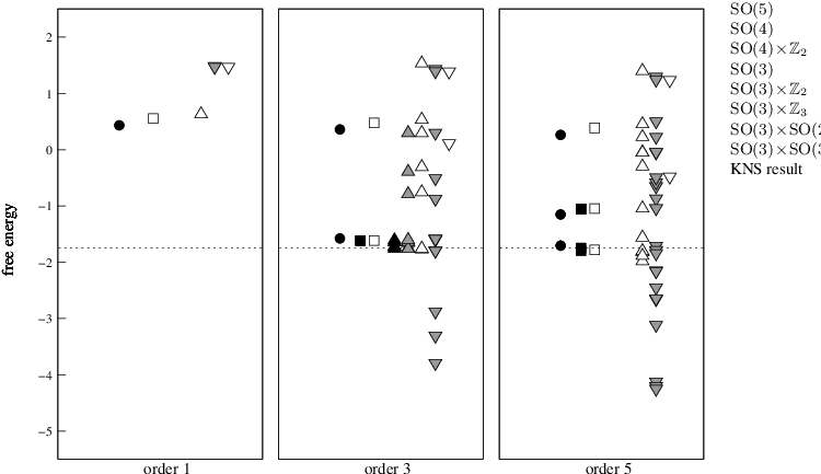
For each Ansatz, we first obtain the free energy up to the 5th order as a function of the parameters in the Gaussian action. By differentiating the free energy with respect to the parameters, we obtain the self-consistency equations, which we solve numerically by Mathematica. The free energy evaluated at each solution is plotted in Fig. 1 for the SO($d$) Ansatz ($d=3,4,5$) described in the previous Section. More precisely, we plot “the free energy density” defined as

$$f=\lim_{N\to\infty}\left\{\frac{F}{N^{2}-1}-\left(-\ln N+\ln 2+1\right)\right\}\ ,$$ (24)

in terms of the free energy $F=-\ln Z$ of the $D=6$ model (1). As we explained in Section 4, solutions can have larger symmetries than the one imposed by the Ansatz. We classify the solutions for each Ansatz by the largest symmetry they actually have.

Figure 1: The free energy density (24) evaluated at solutions of the self-consistency equations at orders 1,3 and 5. Each symbol represents the largest symmetry that the solution has. The dotted line represents the value ($-\frac{7}{4}$) obtained from the KNS conjecture.

order	symmetry	$f$	$\langle\lambda_{1,2,3}\rangle$	$\langle\lambda_{4}\rangle$	$\langle\lambda_{5}\rangle$	$\langle\lambda_{6}\rangle$
1	$\mathop{\rm SO}(5)$	$\phantom{-}0.43323$	$0.46291$	–	–	$0.15430$	$\ast$
	$\mathop{\rm SO}(4)\!\times\!\mathbb{Z}_{2}$	$\phantom{-}0.55517$	$0.50813$	–	$0.31861$	$0.12498$	$\ast$
	$\mathop{\rm SO}(3)\!\times\!\mathbb{Z}_{3}$	$\phantom{-}0.63196$	$0.55965$	$0.36511$	–	$0.07153$	$\ast$
	$\mathop{\rm SO}(3)\!\times\!\mathop{\rm SO}(2)$	$\phantom{-}1.48083$	$0.14434$	$0.86603$	–	$0.43301$
		$\phantom{-}1.46896$	$0.13949$	$0.73581$	–	$0.67952$
	$\mathop{\rm SO}(3)\!\times\!\mathop{\rm SO}(3)$	$\phantom{-}1.46897$	$0.71685$	$0.13950$	–	–
3	$\mathop{\rm SO}(5)$	$-1.57681$	$0.69925$	–	–	$0.18720$	$\ast$
	$\mathop{\rm SO}(4)$	$-1.61405$	$0.87262$	–	$0.26392$	$0.18597$	$\ast$
		$-1.61942$	$0.51325$	–	$2.07517$	$0.18295$
	$\mathop{\rm SO}(4)\!\times\!\mathbb{Z}_{2}$	$-1.61396$	$0.87559$	–	$0.25981$	$0.18587$	$\ast$
	$\mathop{\rm SO}(3)$	$-1.60777$	$0.33740$	$6.98126$	$0.11361$	$0.11036$
		$-1.64285$	$0.59561$	$2.58941$	$0.20836$	$0.17600$
		$-1.72044$	$0.65091$	$1.84641$	$0.33620$	$0.18244$
		$-1.75426$	$0.67863$	$2.43441$	$0.18529$	$0.17919$
	$\mathop{\rm SO}(3)\!\times\!\mathbb{Z}_{2}$	$-1.60108$	$0.35849$	$6.37253$	$6.37253$	$0.12631$
		$-1.63294$	$1.02317$	$0.55197$	$0.24407$	$0.18307$
		$-1.64022$	$0.61060$	$2.31060$	$0.23485$	$0.07816$
		$-1.65519$	$0.28107$	$9.59445$	$0.08448$	$0.07992$
		$-1.74649$	$0.68185$	$2.17747$	$0.21743$	$0.18003$
		$-1.76129$	$1.39517$	$0.21393$	$0.19198$	$0.17947$	$\ast$
	$\mathop{\rm SO}(3)\!\times\!\mathbb{Z}_{3}$	$-1.75564$	$1.37852$	$0.21601$	–	$0.16208$	$\ast$
		$-1.77159$	$1.43148$	$0.20030$	–	$0.15052$	$\ast$
	$\mathop{\rm SO}(3)\!\times\!\mathop{\rm SO}(2)$	$-1.58507$	$0.42282$	$1.29610$	–	$0.17334$
		$-1.58596$	$0.49087$	$1.10749$	–	$0.18127$
		$-1.59755$	$0.88526$	$0.47466$	–	$0.18349$
		$-1.79126$	$1.47103$	$0.18007$	–	$0.18387$	$\ast$
		$-1.79828$	$1.51783$	$0.16939$	–	$0.18120$	$\ast$
5	$\mathop{\rm SO}(5)$	$-1.70472$	$0.78386$	–	–	$0.20789$	$\ast$
	$\mathop{\rm SO}(4)$	$-1.74598$	$0.55629$	–	$2.78951$	$0.19406$
		$-1.79599$	$1.11197$	–	$0.20256$	$0.18450$	$\ast$
	$\mathop{\rm SO}(4)\!\times\!\mathbb{Z}_{2}$	$-1.78072$	$1.01665$	–	$0.27056$	$0.20861$	$\ast$
	$\mathop{\rm SO}(3)\!\times\!\mathbb{Z}_{3}$	$-1.55969$	$1.83885$	$0.19760$	–	$0.14390$
		$-1.79936$	$1.78423$	$0.16467$	–	$0.17362$	$\ast$
		$-1.81743$	$1.67816$	$0.16476$	–	$0.14599$	$\ast$
	$\mathop{\rm SO}(3)\!\times\!\mathop{\rm SO}(2)$	$-1.71169$	$0.71671$	$0.90525$	–	$0.20783$
		$-1.78197$	$1.77827$	$0.32212$	–	$0.11537$
		$-1.84330$	$1.70995$	$0.14987$	–	$0.17730$	$\ast$

Table 1: Numerical values of the free energy density and the eigenvalues of the moment-of-inertia tensor evaluated at the solutions that appear in Fig. 1 for order 1, and at the solutions that appear in Fig. 2 for orders 3 and 5. The dash in some columns for $\langle\lambda_{i}\rangle$ indicates that the value is the same as the one on the left column due to the symmetry of the solution. Asterisks in the right-most column indicate the solutions we consider to be “physical”.

The horizontal dotted line represents the result $f=-\frac{7}{4}=-1.75$ obtained in Appendix B from the analytic formula for the partition function conjectured by Krauth, Nicolai and Staudacher [24] (KNS) combining their Monte Carlo results at small $N$ and earlier analytic works [34, 35]. As we go to higher orders, we obtain many solutions with the free energy density close to the KNS value. We take this as an evidence for the validity of GEM in the present model. In Fig. 2 we zoom up the region near the KNS value. Table 1 shows the numerical values obtained for the free energy density at each solution. For orders 3 and 5, we restrict the solutions to those displayed in Fig. 2.

Figure 2: The same as Fig. 1 except that we zoom up a small region of the free energy density near the KNS value. The data points surrounded by the dashed lines correspond to the concentrating solutions, which indicate the formation of plateaus.

In Table 1 we also present the six eigenvalues of the moment-of-inertia tensor (7), which enable us to probe the extent of space-time in each direction. To obtain these values, we expand the expectation value of the observable (7) by using the formula (18) and evaluate it at the solution of the self-consistency equations (19). Note that the result obtained in this way is not necessarily diagonal. For the $\mathop{\rm SO}(4)$ Ansatz, for instance, it takes the form

$$\langle T_{\mu\nu}\rangle=\left\langle\frac{1}{N}\mathop{\rm Tr}(A_{\mu}A_{\nu})\right\rangle=\begin{pmatrix}C&&&&\vline\\ &C&&&\vline\\ &&C&&\vline\\ &&&C&\vline\\ \hline\cr&&&&\vline&c_{1}&c_{3}\\ &&&&\vline&c_{3}&c_{2}\\ \end{pmatrix}\ .$$ (25)

In such a case, we have to diagonalize the matrix to obtain the eigenvalues.

There are some solutions in Table 1 having smaller values in the directions involved in the preserved $\mathop{\rm SO}(d)$ symmetry than in the remaining directions. Such solutions are discarded and will not be considered in what follows. At orders 3 and 5, we find a set of solutions for $d=3,4$ giving similar values for the free energy density and the eigenvalues $\langle\lambda_{i}\rangle$. We consider this as the concentration of solutions [11], which indicates the formation of plateaus in the space of parameters explained in Section 3. The data points in Fig. 2 corresponding to such solutions are surrounded by the dashed lines. Thus we can pick up the “physical solutions” for each $d$ without much ambiguity, which we have marked by asterisk in the right-most column of Table 1.

Figure 3: The extent of space-time $R^{2}$ and $r^{2}$ in the extended (upper panel) and shrunken directions (lower panel), respectively, evaluated at the “physical solutions” that are marked by asterisk in Table 1.

The free energy density obtained by averaging over the physical solutions for each $d=3,4,5$ at orders 3 and 5 is found to decrease monotonically as $d$ decreases. The deviation from the KNS value is reasonable considering the accuracy of the present method at this order.

It is interesting to note in Table 1 that all the SO(3) symmetric solutions without extra symmetries found at order 3 are actually the ones we decided to discard because of having larger extent in the extra dimensions. Therefore, the fact that we could not study the SO(3) symmetric vacuum at order 5 without imposing extra symmetries actually may not be that harmful in the present analysis. On the other hand, we find in Fig. 1 that the $\mathop{\rm SO}(3)\times\mathop{\rm SO}(3)$ symmetric solutions have larger free energy density and hence do not appear in Fig. 2. This is understandable since the $\mathop{\rm SO}(3)\times\mathop{\rm SO}(3)$ symmetry forces all the $m_{\mu}$’s to vanish, and therefore the situation can be qualitatively different from the other SO(3) symmetric solutions, which have some non-zero components in $m_{\mu}$.

Figure 4: The extent of space-time $R^{2}$ and $r^{2}$ in the extended and shrunken directions, respectively, are plotted at each order by taking an average over the “physical solutions” for each Ansatz.

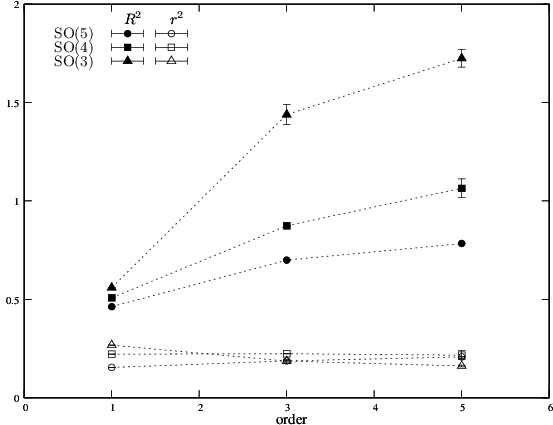
Let us also discuss the results for the extent of space-time. For the $\mathop{\rm SO}(d)$ Ansatz, the $d$ large eigenvalues of $\langle T_{\mu\nu}\rangle$ are equal due to the imposed SO($d$) symmetry, and we denote the value as $R^{2}$. The remaining $(6-d)$ eigenvalues for each “physical solution” turn out to be quite close to each other and we denote the mean value as $r^{2}$. In Fig. 3 we plot the values of $R^{2}$ and $r^{2}$ evaluated at the “physical solutions” for each Ansatz. (Note that the scale is different for the upper and lower panels.) Taking the average within each Ansatz, we obtain the plot in Fig. 4. We put error bars representing the mean square error when there are more than one physical solutions within the Ansatz.

We find that $r^{2}$ is quite stable against increasing the order of the expansion, and it seems to have an approximately universal value $r^{2}\sim 0.2$ for all the SO($d$) symmetric vacua with $d=3,4,5$. On the other hand, we find that $R^{2}$ for each $d$ increases with the order, and the convergence is not clear from this plot alone. However, we observe a clear tendency at each order that $R^{2}$ is larger for smaller $d$ in contrast to the universal behavior of $r^{2}$.

6 Interpretation based on the low-energy effective theory

In this Section we provide a theoretical understanding of the results in the previous Section based on the low-energy effective theory. Let us start from the action (2) and (3), where we keep the scale parameter $g$ unspecified throughout this Section (instead of fixing it by $g^{2}N=1$ as we have been doing so far) to make some arguments clearer. First we decompose the bosonic and fermionic matrices as

$$(A_{\mu})_{ij} = x_{i\mu}\delta_{ij}+a_{\mu ij}\ ,$$ (26)

$$(\Psi_{\alpha})_{ij} = \xi_{i\alpha}\delta_{ij}+\varphi_{\alpha ij}\ ,$$ (27)

$$(\bar{\Psi}_{\alpha})_{ij} = \bar{\xi}_{i\alpha}\delta_{ij}+\bar{\varphi}_{\alpha ij}\ ,$$ (28)

where $a_{\mu ij}$, $\varphi_{\alpha ij}$ and $\bar{\varphi}_{\alpha ij}$ contain only off-diagonal elements. We may view $x_{i\mu}$ as the $\mu$-th coordinate of a point $\vec{x}_{i}$ in $6$-dimensional space-time. When $\sqrt{(\vec{x}_{i}-\vec{x}_{j})^{2}}\gg\sqrt{g}$, namely when all the $N$ points are separated from each other, we can integrate out the off-diagonal parts $a_{\mu ij}$, $\varphi_{\alpha ij}$ and $\bar{\varphi}_{\alpha ij}$ at one loop to obtain the effective action for the diagonal elements $x_{i\mu}$, $\xi_{i\alpha}$ and $\bar{\xi}_{i\alpha}$. If one sets $\xi_{i\alpha}=\bar{\xi}_{i\alpha}=0$, the effective action actually vanishes as a consequence of supersymmetry. However, the integration over $\xi_{i\alpha}$ and $\bar{\xi}_{i\alpha}$ induces a branched-polymer-like interaction for $x_{i\mu}$ [4].

Let us briefly review this calculation. Adding the gauge fixing term corresponding to the Feynman gauge, one obtains the bosonic action relevant at one loop as

$$S_{\rm b,1-loop}=\frac{1}{g^{2}}\sum_{i<j}(\vec{x}_{i}-\vec{x}_{j})^{2}|a_{\mu ij}|^{2}\ .$$ (29)

If we set $\xi_{i\alpha}=0$, the fermionic action relevant at one loop becomes

$$S_{\rm f,1-loop}(\xi=\bar{\xi}=0)=-\frac{1}{g^{2}}(\Gamma_{\mu})_{\alpha\beta}\sum_{i\neq j}(x_{i\mu}-x_{j\mu})\bar{\varphi}_{\alpha ji}\varphi_{\beta ij}\ .$$ (30)

Let us first integrate over the bosonic variables ($a_{\mu ij}$). Including the factor $\{\Delta(x)\}^{2}$ coming the Faddeev-Popov determinant associated with the gauge fixing, where

$$\Delta(x)=\prod_{i<j}(\vec{x}_{i}-\vec{x}_{j})^{2}\ ,$$ (31)

we obtain a factor $\{\Delta(x)\}^{-4}$, which represents an attractive potential between every pair of $\vec{x}_{i}$. We can easily see that the integration over the fermionic variables ($\varphi_{\alpha ij}$ and $\bar{\varphi}_{\alpha ij}$) yields a factor $\{\Delta(x)\}^{4}$, which exactly cancels the attractive potential induced by the bosonic variables.

Let us then consider what happens if we do not set $\xi_{i\alpha}=\bar{\xi}_{i\alpha}=0$. Here we follow the formulation in Ref. Ambjorn:2000dx. The fermionic part of the action (3) relevant at one loop reads

$$S_{\rm f,1-loop} = -\frac{1}{g^{2}}\,(\Gamma_{\mu})_{\alpha\beta}\sum_{i\neq j}\Bigl\{(x_{i\mu}-x_{j\mu})\bar{\varphi}_{\alpha ji}\varphi_{\beta ij}$$ (32)

$$\quad\quad\quad\quad\quad\quad-\bar{\varphi}_{\alpha ji}(\xi_{i\beta}-\xi_{j\beta})a_{\mu ij}-a_{\mu ji}(\bar{\xi}_{i\alpha}-\bar{\xi}_{j\alpha})\varphi_{\beta ij}\Bigl\}\ .$$

Completing the square with respect to $\varphi_{\alpha ij}$ and $\bar{\varphi}_{\alpha ij}$, and integrating over them, one obtains a factor $\{\Delta(x)\}^{4}$ we encountered above. The remaining term in the action is given by

$$\tilde{S}_{\rm f,1-loop}=-\frac{1}{g^{2}}\,\sum_{ij}\bar{\xi}_{i\alpha}M_{i\alpha,j\beta}\xi_{j\beta}\ ,$$ (33)

where $M_{i\alpha,j\beta}$ is a $4N$ $\times$ $4N$ matrix given as

$$M_{i\alpha,j\beta} = \frac{(x_{i\rho}-x_{j\rho})}{(\vec{x}_{i}-\vec{x}_{j})^{2}}(\Gamma_{\mu}\Gamma_{\rho}^{\dagger}\Gamma_{\sigma})_{\alpha\beta}(a_{\mu ji}a_{\sigma ij}-a_{\mu ij}a_{\sigma ji})~~~~~\mbox{for}~~~i\neq j\ ,$$ (34)

$$M_{i\alpha,i\beta} = -\sum_{j\neq i}M_{i\alpha,j\beta}\ .$$ (35)

Integration over $\xi_{i\alpha}$ and $\bar{\xi}_{i\alpha}$ gives the determinant $\det\,M$, which represents an attractive force between $x_{i\mu}$ and $x_{j\nu}$ connected by a bond in a branched polymer as one can see from the definition of determinants. In order for the one-loop approximation to be valid, we have to impose $|\vec{x}_{i}-\vec{x}_{j}|>a_{\rm cut}$ for all $i\neq j$. The cutoff $a_{\rm cut}\sim\sqrt{g}$ is expected to appear dynamically through the non-perturbative effects of the off-diagonal elements [26]. The bond length of the branched polymer is given approximately by $a_{\rm bond}\sim a_{\rm cut}$.

The determinant $\det\,M$ is complex, and the phase factor actually plays an important role in the SSB of SO(6). However, let us for the moment consider the dynamics of a system with $|\det\,M|$ omitting the phase. Due to general properties of a branched polymer, the extent of the distribution of points is given by $\ell=O(a_{\rm bond}N^{1/4})$, where $N$ gives the number of points in the branched polymer. Thus we obtain $\ell\sim\sqrt{g}N^{1/4}$ as first predicted in Ref. Aoki:1998vn. This property has been confirmed by Monte Carlo simulations for the $D=6,10$ models [23] using the one-loop approximation, and for the $D=4$ model [26] without using the one-loop approximation.

As we mentioned in Section 2, the phase of the determinant favors collapsed configurations, and the branched-polymer structure will be flattened by this effect. Since the interactions among $x_{i\mu}$ through the branched polymer structure is O($1/N$) suppressed (Note that there are only O($N$) number of bonds.), it is conceivable that the diagonal part of (26) is totally suppressed in the shrunken directions, and that in those directions, one only sees the fluctuation of the off-diagonal part $a_{\mu ij}$, which is mostly determined by the Gaussian term (29). Since the coefficient $(\vec{x}_{i}-\vec{x}_{j})^{2}$ in the Gaussian term (29) is rotationally invariant, the fluctuation of $a_{\mu ij}$ is insensitive to the SO(6) breaking in the distribution of $\vec{x}_{i}$. This explains why we obtain similar extents in all shrunken directions for each Ansatz. Moreover since the magnitude of the coefficient $(\vec{x}_{i}-\vec{x}_{j})^{2}$ is set by the typical length scale $\ell$ of the branched polymer, it is also understandable that the mean extent in the shrunken directions is universal for all the SO($d$) symmetric vacuum with $d=3,4,5$. The flattening of the branched polymer may cause some $d$-dependence through (29) in principle, but the observed universality suggests that this effect is small.

Figure 5: The extent of space-time $R^{2}$ in units of $g\sqrt{N}$ is plotted in the log scale against $1/d$. The solid straight line is a linear fit to the results at order 5, from which we obtain $\tilde{r}^{2}/g\sqrt{N}=0.223$ and $\ell^{2}/g\sqrt{N}=0.627$ in Eq. (37).

Let us now turn our attention to the extent $R^{2}$ in the extended directions, which we denote here as $(R_{d})^{2}$ to make its $d$-dependence manifest. From entropic reasons, we may naively expect that the branched polymer tends to occupy a fixed volume in $D$ dimensions, which implies that

$$(R_{d})^{d}(\tilde{r})^{D-d}\approx\ell^{D}\ ,$$ (36)

where $\ell$ represents the extent of space-time in the model omitting the phase of the determinant. The parameter $\tilde{r}$ represents the extent in the shrunken directions, which we assume to be the same for all $d=3,4,5$ based on the universality discussed above, but leave its value to be unknown here. This leads to

$$(R_{d})^{2}\approx\tilde{r}^{2}\left(\frac{\ell^{2}}{\tilde{r}^{2}}\right)^{D/d}\ .$$ (37)

To test this behavior in the present $D=6$ case, we plot in Fig. 5 the results for $(R_{d})^{2}$ obtained by GEM (with $g^{2}N=1$) in the log scale against $1/d$. Indeed we find that the results tend to lie on a straight line as expected from (37) as we increase the order. By fitting the order 5 results to (37), we obtain $\tilde{r}^{2}/(g\sqrt{N})=0.223$ and $\ell^{2}/(g\sqrt{N})=0.627$. Note that the value of $\tilde{r}^{2}/(g\sqrt{N})$ obtained from this analysis turns out to be consistent with the extent in the shrunken directions $r^{2}\sim 0.2$ obtained by GEM directly with $g^{2}N=1$, which is quite nontrivial.

We may consider $\ell^{2}/(g\sqrt{N})=0.627$ as a prediction from the present argument. We can obtain it by Monte Carlo simulation of the $D=6$ model omitting the phase of the fermion determinant. The values of the $\lambda_{i}/(g\sqrt{N})$ ($1\leq i\leq 6$) are obtained up to $N=32$, and they all seem to converge to some value around 0.6 in the large-$N$ limit assuming the finite-$N$ effects to be of O($1/N$)[36]. This also supports the validity of the constant volume property (36).

The extent in the shrunken directions being stable against increasing the order of the Gaussian expansion can be understood from the fact that we are essentially seeing the fluctuation of the off-diagonal elements, which are governed by an action like (29). On the other hand, the slow convergence of the extent in the extended directions can be understood from the fact that we are essentially seeing the fluctuation of the diagonal elements governed by the branched-polymer dynamics. The distribution of $\vec{x}_{i}$ tends to be uniform, which is not well described by the Gaussian action. From this point of view, it is expected that the convergence becomes slower for smaller $d$ since $(R_{d})^{2}$ becomes larger according to (37).

7 Results for the SO(2) symmetric vacuum

Figure 6: The free energy density for the SO($d$) symmetric vacuum obtained in this work is plotted against $d$. The horizontal dashed line represents the KNS value $f=-7/4$, and the dotted line connecting the data points is drawn to guide the eye.

In this Section we present some results for the SO(2) symmetric vacuum. Since we have 13 parameters in the Gaussian action for the SO(2) symmetric vacuum, we decided to impose $\mbox{SO(2)}\times\mathbb{Z}_{4}$ symmetry as we discussed in Section 4. Considering the results for the SO(3) symmetric vacuum discussed in Section 5, we expect that imposing the extra $\mathbb{Z}_{4}$ symmetry may not be that harmful.

In Table 2 we present the solutions of the self-consistency equations. At order 5 we find two solutions (marked by asterisk in the right-most column) which have the extent in the shrunken directions consistent with our result $r^{2}\sim 0.2$ obtained for the SO($d$) symmetric vacua with $d=3,4,5$ universally. The extent in the extended directions obtained for these solutions is $(R_{2})^{2}=2.3\sim 2.6$, which is larger than those obtained for the SO(3) symmetric vacuum at the same order. Assuming that the universality extends to SO(2), we may consider these marked solutions at order 5 as the physical ones. Then an estimate of the free energy density for the SO(2) symmetric vacuum is obtained as $f=-0.25\sim-0.27$ from Table 2, which is considerably larger than the free energy density for the SO($d$) symmetric vacuum with $d=3,4,5$. This is consistent with the argument that the 2d space-time is suppressed by the fermion determinant [20].

order	symmetry	$f$	$\langle\lambda_{1,2}\rangle$	$\langle\lambda_{3,4,5}\rangle$	$\langle\lambda_{6}\rangle$
3	$\mathop{\rm SO}(2)\!\times\!\mathbb{Z}_{4}$	$\phantom{-}2.29076$	$0.13771$	$0.82660$	$1.60667$
		$\phantom{-}1.66758$	$1.32164$	$0.18382$	$0.15111$
		$\phantom{-}0.10128$	$1.06136$	$0.20591$	$0.42461$
		$-2.35965$	$1.81697$	$0.26882$	$0.48377$
		$-2.42857$	$1.72922$	$0.21400$	$0.44805$
		$-2.81818$	$3.95383$	$0.12571$	$0.13949$
		$-3.27169$	$5.85293$	$0.08432$	$0.10029$
		$-3.31790$	$4.74086$	$0.12446$	$0.14714$
5	$\mathop{\rm SO}(2)\!\times\!\mathbb{Z}_{4}$	$\phantom{-}2.13955$	$0.14119$	$0.87447$	$1.72675$
		$\phantom{-}1.51355$	$1.51225$	$0.18530$	$0.15941$
		$\phantom{-}0.16798$	$2.83645$	$0.12589$	$0.13595$
		$-0.13712$	$3.18237$	$0.12008$	$0.11814$
		$-0.25243$	$2.29020$	$0.16355$	$0.17833$	$\ast$
		$-0.27313$	$2.57212$	$0.14915$	$0.15902$	$\ast$
		$-1.18723$	$6.87681$	$0.04775$	$0.03738$
		$-1.22564$	$7.25959$	$0.04115$	$0.01773$
		$-2.45562$	$11.8953$	$0.03757$	$0.04213$
		$-2.63861$	$12.1413$	$0.03970$	$0.04170$
		$-2.92543$	$13.7449$	$0.03624$	$0.03723$
		$-3.55149$	$0.42405$	$0.46966$	$0.45653$
		$-3.57951$	$8.75022$	$0.05582$	$0.06260$
		$-3.6158$	$0.29921$	$0.73480$	$0.36202$
		$-3.90928$	$9.94824$	$0.04923$	$0.05356$
		$-4.11550$	$5.17586$	$0.10051$	$0.10911$
		$-4.20561$	$6.79049$	$0.07689$	$0.08446$
		$-12.1677$	$0.19044$	$1.53911$	$1.77276$

Table 2: Numerical values of the free energy density and the eigenvalues of the moment-of-inertia tensor evaluated at the solutions obtained for the $\mbox{SO(2)}\times\mathbb{Z}_{4}$ Ansatz. Asterisks in the right-most column indicate the solutions we consider to be “physical”.

In Fig. 6 we plot the free energy density for the SO($d$) symmetric vacuum against $d$. (When there are more than one “physical solutions” we take the average and put an error bar representing the mean square error as in Fig. 4.) Thus we conclude that the SO(3) symmetric vacuum gives the smallest free energy, and hence it is chosen as the true vacuum.

8 Reconsideration of the $D=10$ case

In this Section we use the new insights obtained from the study of the $D=6$ case to reconsider the previous results obtained by GEM in the $D=10$ case. Fig. 7 shows the results for the $D=10$ model up to the 5th order taken from Ref. Kawai:2002ub. In order to reduce the number of arbitrary parameters, two types of symmetry were imposed. One is the $\mathop{\rm SO}(7)\!\times\!\mathop{\rm SO}(3)$ symmetry, and the other is the $\mathop{\rm SO}(4)\!\times\!\mathop{\rm SO}(3)\!\times\!\mathop{\rm SO}(3)\!\times\!\mathbb{Z}_{2}$ symmetry, where $\mathbb{Z}_{2}$ corresponds to interchanging the two $\mathop{\rm SO}(3)$.

For the SO(4) Ansatz, we find that solutions No.3 and No.5 at order 5 give similar values for all the quantities, which we consider as an indication of the plateau formation. For the SO(7) Ansatz, we take the solution No.3 to be the physical one considering the similarity of the pattern to what we have observed for the SO(5) symmetric vacuum in the $D=6$ model; See Fig. 1. Note also that the values of free energy density obtained for the “physical solutions” we picked up above are quite close to the KNS value represented by the horizontal dotted line.

Then we find that the situation is actually quite similar to the $D=6$ case. First the free energy density is smaller for the SO(4) symmetric vacuum than for the SO(7) symmetric vacuum. The extent of space-time in the shrunken directions is around $r^{2}=0.13\sim 0.15$ for both vacua. On the other hand, the extent of space-time in the extended directions is estimated as $(R_{4})^{2}=1.6\sim 1.8$ for the SO(4) symmetric vacuum and $(R_{7})^{2}=0.52\sim 0.65$ for the SO(7) symmetric vacuum.

Assuming the formula (36) to hold also in the $D=10$ model and using the values of $(R_{d})^{2}$ extracted above, we can put constraints on $\ell^{2}$ and $\tilde{r}^{2}$ as shown in Fig. 8. We also indicate the region of $\tilde{r}^{2}$ suggested from the extent of space-time in the shrunken directions $r^{2}=0.13\sim 0.15$ obtained directly by GEM. Quite nontrivially, we find a region in which all the three constraints are satisfied. The allowed region for $\ell^{2}$ turns out to be $\ell^{2}=0.35\sim 0.4$. As in the $D=6$ case, we expect that this value can be reproduced by calculating the extent of space-time in the model omitting the phase of the fermion determinant. Preliminary results of Monte Carlo simulation for $D=10$ suggest that this is indeed the case [36]. We therefore consider that the values of observables extracted above from the physical solutions are sensible. Note, in particular, that we have $R_{4}/r=3.3\sim 3.7$, which is finite as opposed to previous speculation that the ratio might be infinite from the results at higher orders [13]. Plugging $r^{2}=0.13\sim 0.15$ and $\ell^{2}=0.35\sim 0.40$ into Eq. (37), we can also predict the values of $(R_{d})^{2}$ for $d$ other than $d=4,7$.

Thus we think that we have arrived at comprehensive understanding on the dynamics of “space-time” in dimensionally reduced super Yang-Mills models for both $D=6$ and $D=10$.

Figure 7: The results for the $D=10$ model obtained by GEM up to the 5th order taken from Ref. Kawai:2002ub. The free energy density (top), the extent of space-time $R^{2}$ in the extended directions (middle) and $r^{2}$ in the shrunken directions (bottom) are plotted against the order of GEM for the $\mathop{\rm SO}(4)$ Ansatz (left column) and the $\mathop{\rm SO}(7)$ Ansatz (right column) with additional symmetries described in the text. The horizontal dotted lines in the top panels represent the KNS value ($\ln 8-\frac{3}{4}=1.32944$) for the $D=10$ model obtained in Ref. Nishimura:2001sx. The arrows with a number are added to identify solutions obtained at each order.

Figure 8: Constraints on $\tilde{r}^{2}$ and $\ell^{2}$ from the formula (36) with the input of the extent of space-time in the extended directions obtained by GEM in the $D=10$ case for the SO($4$) symmetric vacuum (the region between the two dash-dotted lines) and the SO($7$) symmetric vacuum (the region between the two dashed lines). The vertical solid lines represent the range of $r^{2}$ (the extent of space-time in the shrunken directions) obtained by GEM directly. There is a region in which all the three constraints are satisfied.

9 Summary and discussions

We have discussed the SSB of SO($D$) in the large-$N$ reduced models obtained by the zero-volume limit of pure SU($N$) super Yang-Mills theories in $D=6,10$ dimensions. Both models have a complex fermion determinant, which is expected to play a crucial role in the conjectured SSB [20, 18, 19, 29].

First we studied the $D=6$ model by GEM up to the 5th order. Unlike the previous studies of the $D=10$ model, we were able to examine the SO($d$) symmetric vacua with $d=3,4,5$ without imposing ad hoc symmetries in the extra dimensions in most cases. From a set of solutions to the self-consistency equations giving results close to each other, clear indication of the plateau formation was observed. This enabled us to obtain reliable results for the free energy and the extent of space-time in each direction as in an analogous study of the toy model [19].

We found that the free energy decreases as we go from $d=5$ to $d=3$. In fact it was argued in Ref. Aoki:1998vn that a branched polymer is difficult to collapse to a hypersurface with less than four dimensions, since the Hausdorff dimension of such a system is four. The reason why our conclusion can still be true is that the system has a finite extent in the shrunken directions for fixed $g^{2}N$. Namely the branched polymer is not really collapsed to a hypersurface.

In fact we found that the shrunken directions have approximately the same extents for $d=3,4,5$. We have given a theoretical explanation of this behavior based on the low-energy effective theory. On the other hand, the extended directions have a larger extent for smaller $d$, and this $d$-dependence can be nicely explained by the law of constant volume (36). From this observation, we obtained a prediction for the extent of space-time in the phase-quenched model (i.e., the model obtained by omitting the phase of the fermion determinant), which seems to be consistent with some preliminary results obtained by Monte Carlo simulation.

The results for the SO(2) symmetric vacua are not clear possibly due to the extra symmetries we had to impose in the extra dimensions. However, if we assume that the extent of space-time in the shrunken directions is close to what we obtained for $d=3,4,5$, we obtain the value of free energy much larger than the values obtained for $d=3,4,5$. This is consistent with the suppression of two-dimensional space-time due to the fermion determinant [20]. Thus we conclude that the SO(6) symmetry of the $D=6$ model is spontaneously broken down to SO(3).

The new insights obtained from the $D=6$ model enabled us to reinterpret the previous results for the $D=10$ model. In particular, we considered the results for the SO(4) and SO(7) symmetric vacua obtained at the 5th order. We found that the extent in the shrunken directions is similar for the two vacua. Assuming the constant volume property (36) and using the extent in the extended directions as an input, we obtained the possible region for $\tilde{r}^{2}$ and $\ell^{2}$. It turned out that the value of $\tilde{r}^{2}$ suggested by this analysis is consistent with the extent in the shrunken directions obtained by GEM directly. The value of $\ell^{2}$, on the other hand, provides a prediction for the extent of the space-time in the phase-quenched model, which is also consistent with some preliminary results of Monte Carlo simulation.

The free energy in the $D=10$ model was calculated for $d=2$, $4$, $6$, $7$ at the 3rd order, and $d=4$ was found to give the minimum.[5] The particular pattern of the $d$-dependence obtained at this order might already capture the correct qualitative behavior considering the results obtained at the 5th order for $d=4$ and $d=7$. This $d$-dependence is similar to what we obtained in the $D=6$ model up to the 5th order, where $d=3$ gives the minimum. In order to determine the true vacuum of the $D=10$ model, we therefore consider it important to compare the free energy for $d=3$, $4$, $5$, including the $d=3$ and $5$ cases which have not been studied so far.

As is discussed in Refs. NV,Nishimura:2001sq,Nishimura:2004ts, the SSB of SO($D$) is caused by the phase of the fermion determinant. Rotationally symmetric configurations are strongly suppressed due to cancellations caused by the violent fluctuation of the phase, whereas the fluctuation becomes milder for collapsed configurations. Monte Carlo studies of these models are difficult precisely because of the cancellations. However, a new method to sample efficiently the dominant configurations including the effects of the phase is proposed in Ref. sign. It is interesting to study the $D=6$ and $D=10$ models by the Monte Carlo method to see whether the results and predictions obtained in this paper can be reproduced. We expect that the method will eventually enable us to reach a definite conclusion on which value of $d$ is chosen dynamically in the $D=10$ model.

To conclude, we consider it interesting that the SSB of SO(6) down to SO(3) has been demonstrated clearly in the $D=6$ model. Our results make it very plausible that an analogous SSB occurs in the $D=10$ model, and that the SO(10) symmetry is broken down to either SO(3), SO(4) or SO(5). This strongly supports the speculation that the IIB matrix model may provide the dynamical origin of the space-time dimensionality. The space-time picture that emerged from the present work is also interesting. The extra dimensions are totally dominated by fluctuations of off-diagonal elements, and presumably do not allow ordinary geometric descriptions. This may provide certain basis for phenomenological models [37] with non-commutative extra dimensions. The space-time in the extended directions is uniform and it is described mostly by the commutative degrees of freedom.

On the other hand, the constant volume property (36) suggested by our results implies that the ratio $R/r$ of the extent of space-time in the extended directions and that in the shrunken directions is finite as opposed to previous speculations that it might be infinite [13]. We feel that this gives us an important clue on how we should actually interpret the IIB matrix model as a non-perturbative definition of type IIB superstring theory. A possible interpretation would be that the model actually describes the state of the early universe in the spirit of Hartle-Hawking [38] as suggested by the fact that the model uses the Euclidean signature for the space-time [7]. From this point of view, it might be interesting to consider a matrix model which incorporates the Lorentzian signature for the space-time, or a matrix model which includes the time from the outset (instead of generating it dynamically) as in the BFSS matrix model [1]. In any case we hope that our findings in this paper motivate further investigations of the matrix model approach to non-perturbative aspects of superstring theories and the origin of our space-time.

Appendix A Symplectic Majorana-Weyl spinors in 6d

In $D=6$ one cannot define Majorana spinors, but one can define symplectic Majorana spinors, and impose the Weyl condition simultaneously.

Let $\psi$ be a Weyl spinor with positive chirality. Its charge conjugation $\psi_{\rm c}$ can be defined by

$$\psi_{\rm c}=C^{-1}\bar{\psi}^{T}\ ,$$ (38)

where $C$ is the charge conjugation matrix satisfying $C\Gamma_{\mu}C^{-1}=(\Gamma_{\mu})^{T}$ and $C^{T}=-C$. Then we define symplectic Majorana-Weyl spinors as

$$\psi_{1} = \frac{1}{2}(\psi-\psi_{\rm c})\ ,$$ (39)

$$\psi_{2} = \frac{1}{2}(\psi+\psi_{\rm c})\ .$$ (40)

It is conventional to define

$$\overline{\psi}^{\,i}=\psi_{i}^{\dagger}\Gamma^{0}\quad(i=1,2)\ .$$ (41)

In this notation, we have

$$(\overline{\psi}^{i})^{T}=C\psi^{i}\ ,$$ (42)

where

$$\psi^{i}=\epsilon^{ij}\psi_{j}\ ,\quad\psi_{j}=\psi^{i}\epsilon_{ij}\ ,\quad\epsilon^{12}=\epsilon_{12}=+1\ .$$ (43)

The symplectic indices are raised and lowered by contracting with $\epsilon^{ij}$ and $\epsilon_{ij}$, respectively, according to the NW-SE rule.

Let us decompose fermionic variables $\Psi_{\alpha}$ in (3) into

$$\Psi_{\alpha}=\Psi_{1,\alpha}+\Psi_{2,\alpha}\ ,$$ (44)

where $\Psi_{1,\alpha}$, $\Psi_{2,\alpha}$ are the components of symplectic Majorana-Weyl spinor. Then, the fermionic part of the original action (3) and the Gaussian action (12) can be rewritten, respectively, as

$$S_{\rm f} = N\mathop{\rm Tr}(\Psi_{i,\alpha}\epsilon^{ij}(C\Gamma^{\mu})_{\alpha\beta}[X_{\mu},\Psi_{j,\beta}])\ ,$$ (45)

$$S_{\rm 0f} = N\sum_{\alpha,\beta=1}^{4}\mathcal{A}^{ij}_{\alpha\beta}\mathop{\rm Tr}(\Psi_{i,\alpha}\Psi_{j,\beta})\ ,$$ (46)

$$\mathcal{A}^{ij}_{\alpha\beta} = (\sigma_{3})^{ij}\sum_{\mu=1}^{6}m_{\mu}(C\Gamma_{\mu})_{\alpha\beta}+\frac{i}{2\cdot 3!}\epsilon^{ij}\!\!\!\!\sum_{\mu,\nu,\rho=1}^{6}m_{\mu\nu\rho}(C\Gamma_{\mu}\Gamma_{\nu}^{\dagger}\Gamma_{\rho})_{\alpha\beta}\ ,$$ (47)

where $m_{\mu}$ and $m_{\mu\nu\rho}$ are the parameters introduced in (13).

By using the symplectic Majorana-Weyl spinors instead of Weyl spinors, one can get rid of the orientation of the fermion propagators, and therefore the number of Feynman diagrams is reduced considerably. In fact the list of Feynman diagrams to be considered is exactly the same as in the IIB matrix model. The summation over the symplectic indices for each diagram can be done very easily.

Appendix B Free energy from the Krauth-Nicolai-Staudacher conjecture

In this Appendix we describe the analytic formula for the partition function conjectured by Krauth, Nicolai and Staudacher (KNS) [24] combining their Monte Carlo results at small $N$ [24] and earlier analytic works [34, 35]. For the present model, the formula reads

$$Z_{\rm KNS} = \int\mbox{d}A\,\mbox{d}\Psi\,\mbox{d}\overline{\Psi}\,e^{-S_{\rm KNS}}\$$ (48)

$$= \dfrac{2^{\frac{N(N+1)}{2}}\pi^{\frac{N-1}{2}}}{2\sqrt{N}\prod_{k=1}^{N-1}k!}\times\frac{1}{N^{2}}\ ,$$

$$S_{\rm KNS} = \frac{2}{N}(S_{\rm b}+S_{\rm f})\ ,$$ (49)

where $S_{\rm b}$ and $S_{\rm f}$ are defined by (2) and (3), respectively. In the above formula, the definition of the action $S_{\rm KNS}$ differs from our definition by the factor of $2/N$. In order to absorb this factor, we introduce the rescaled variables $A^{\prime}_{\mu}=(2/N)^{1/4}A_{\mu}$, $\Psi^{\prime}_{\alpha}=(2/N)^{3/8}\Psi_{\alpha}$ and $\bar{\Psi}^{\prime}_{\alpha}=(2/N)^{3/8}\bar{\Psi}_{\alpha}$, whose integration measure is given by

$$\mbox{d}A^{\prime}\,\mbox{d}\Psi^{\prime}\,\mbox{d}\overline{\Psi}^{\prime}=\left(\frac{N}{2}\right)^{\frac{3}{2}(N^{2}-1)}\mbox{d}A\,\mbox{d}\Psi\,\mbox{d}\overline{\Psi}\ .$$ (50)

As a result, the partition function (1) can be obtained as

$$Z = \left(\frac{N}{2}\right)^{\frac{3}{2}(N^{2}-1)}Z_{\rm KNS}$$ (51)

$$= 2^{-N^{2}-\frac{N}{2}-\frac{5}{2}}\pi^{\frac{N-1}{2}}N^{\frac{3}{2}N^{2}-4}\prod_{k=1}^{N-1}k!\ .$$

From this, we obtain the large-$N$ asymptotics as

$$\frac{F}{N^{2}-1}=-\ln N+\ln 2-\frac{3}{4}+O\left(\frac{\ln N}{N^{2}}\right)\ .$$ (52)

GEM reproduces the first term correctly for any Ansatz. Substituting this into the definition (24) of the “free energy density”, we obtain $f=-\frac{7}{4}=-1.75$ as a prediction from the KNS conjecture.

References

- [1] T. Banks, W. Fischler, S. H. Shenker, and L. Susskind, \PRD55,1997,5112.
- [2]
N. Ishibashi, H. Kawai, Y. Kitazawa, and A. Tsuchiya,
\NPB498,1997,467.
H. Aoki, S. Iso, H. Kawai, Y. Kitazawa, A. Tsuchiya and T. Tada, \PTPS134,1999,47. - [3] R. Dijkgraaf, E. P. Verlinde, and H. L. Verlinde, \NPB500,1997,43.
- [4] H. Aoki, S. Iso, H. Kawai, Y. Kitazawa, and T. Tada, \PTP99,1998,713.
- [5] J. Nishimura and F. Sugino, \JHEP05,2002,001.
- [6] H. Kaneko, Y. Kitazawa and D. Tomino, \NPB725,2005,93.
- [7] H. Kaneko, Y. Kitazawa and D. Tomino, \PRD73,2006,066001.
- [8] H. Itoyama and R. Yoshioka, \NPB823,2009,254.
- [9] H. Steinacker, Class. Quant. Grav. 27 (2010), 133001.
- [10] J. Lee and H. S. Yang, arXiv:1004.0745.
- [11] H. Kawai, S. Kawamoto, T. Kuroki, T. Matsuo, and S. Shinohara, \NPB647,2002,153.
- [12] H. Kawai, S. Kawamoto, T. Kuroki, and S. Shinohara, \PTP109,2003,115.
- [13] T. Aoyama and H. Kawai, \PTP116,2006,405.
- [14] T. Aoyama and Y. Shibusa, \NPB754,2006,48.
- [15] T. Aoyama, H. Kawai, and Y. Shibusa, \PTP115,2006,1179.
- [16] J. Nishimura, T. Okubo, and F. Sugino, \JHEP10,2002,043.
- [17] J. Nishimura, T. Okubo, and F. Sugino, \JHEP10,2003,057.
- [18] J. Nishimura, \PRD65,2002,105012.
- [19] J. Nishimura, T. Okubo, and F. Sugino, \PTP114,2005,487.
- [20] J. Nishimura and G. Vernizzi, \JHEP04,2000,015; \PRL85,2000,4664.
- [21] Y. Kitazawa, S. Mizoguchi, and O. Saito, \PRD74,2006,046003.
- [22]
M. Berkooz, M. Rozali, and N. Seiberg,
\PLB408,1997,105.
N. Seiberg, \PLB408,1997,98. - [23] J. Ambjorn, K. N. Anagnostopoulos, W. Bietenholz, T. Hotta, and J. Nishimura, \JHEP07,2000,011.
- [24] W. Krauth, H. Nicolai, and M. Staudacher, \PLB431,1998,31.
- [25] P. Austing and J. F. Wheater, \JHEP02,2001,028; \andvol04,2001,019.
- [26] J. Ambjorn, K. N. Anagnostopoulos, W. Bietenholz, T. Hotta, and J. Nishimura, \JHEP07,2000,013.
- [27] Z. Burda, B. Petersson, and J. Tabaczek, \NPB602,2001,399.
- [28] J. Ambjorn, K. N. Anagnostopoulos, W. Bietenholz, F. Hofheinz, and J. Nishimura, \PRD65,2002,086001.
- [29] K. N. Anagnostopoulos and J. Nishimura, \PRD66,2002,106008.
- [30] D. Kabat and G. Lifschytz, \NPB571,2000,419.
- [31]
D. Kabat, G. Lifschytz and D. A. Lowe,
\PRL86,2001,1426.
D. Kabat, G. Lifschytz and D. A. Lowe, \PRD64,2001,124015.
N. Iizuka, D. Kabat, G. Lifschytz, and D. A. Lowe, \PRD65,2002,024012. - [32]
S. Oda and F. Sugino,
\JHEP03,2001,026.
F. Sugino, \JHEP07,2001,014. - [33] P. M. Stevenson, \PRD23,1981,2916.
- [34] M. B. Green and M. Gutperle, \JHEP01,1998,005.
- [35] G. W. Moore, N. Nekrasov, and S. Shatashvili, \CMP209,2000,77.
- [36] K. N. Anagnostopoulos, T. Aoyama, T. Azuma, M. Hanada, and J. Nishimura, work in progress.
- [37] A. Chatzistavrakidis, H. Steinacker and G. Zoupanos, \JHEP05,2010,100.
- [38] J. B. Hartle and S. W. Hawking, \PRD28,1983,2960.
- [39] M. Fukuma, H. Kawai, Y. Kitazawa and A. Tsuchiya, \NPB510,1998,158.
- [40] H. Kawai and M. Sato, \PLB659,2008,712.