Towards a Loop–Tree Duality at Two Loops and Beyond

Abstract

We present an extension of the duality theorem, previously defined by S. Catani et al on the one–loop level, to higher loop orders. The duality theorem provides a relation between loop integrals and tree–level phase–space integrals. Here, the one–loop relation is rederived in a way which is more suitable for its extension to higher loop orders. This is shown in detail by considering the two–loop N–leg master diagram and by a short discussion of the four master diagrams at three loops, in this sketching the general structure of the duality theorem at even higher loop orders.

1 INTRODUCTION

Theoretical predictions of high precision for background and signal multi–particle hard scattering processes in the Standard Model (SM) and beyond, are mandatory in the era after the start of the LHC. To achieve this high level of precision, one needs to compute cross sections at next-to-leading order (NLO), or even next-to-next-to leading order (NNLO). However, going to higher orders in perturbation theory, as well as increasing the number of external particles for the consideration of multi–particle processes, both lead to an increase in complexity of the calculations and of the challenges one has to face in doing the numerical evaluations. In recent years, important efforts have been devoted to developing efficient methods for the calculation of multi–leg and multi–loop diagrams, realized, e.g., by unitarity–based methods or by traditional Feynman diagram approaches, [1].

The computation of cross sections at NLO (or NNLO) requires the separate evaluation of real and virtual radiative corrections, which are given in the former case by multi–leg tree–level and in the latter by multi–leg loop matrix elements to be integrated over the multi–particle phase–space of the physical process. The loop–tree duality at one–loop presented in Ref. [2], as well as other methods relating one–loop and phase–space integrals, [3, 4, 5], recast the virtual radiative corrections in a form that closely parallels the contribution of the real radiative corrections. The use of this close correspondence is meant to simplify calculations through a direct combination of real and virtual contributions to NLO cross sections. Furthermore, the duality relation has analogies with the Feynman Tree Theorem (FTT), [6, 7], but offers the advantage of involving only single cuts of the one–loop Feynman diagrams.

In this talk, the extension of the loop–tree duality theorem derived in Ref. [2] to higher loop orders is described, with the aim of extending the duality method to the computation of cross sections at NNLO or even higher orders. This has been explained in detail in Ref. [8]. The higher–order dual representations described here are valid as long as only single poles are present when the residue theorem is applied (cf.Section 3). At two– or higher loop orders, however, higher order poles might appear which require a separate treatment which is beyond the scope of the current talk.

2 THE DUAL PROPAGATOR $G_{D}$

We first state some necessary definitions and introduce the basic formulae used in the following, leading to the main relation Eq. (2) which is fundamental for the extension of the duality theorem to higher loop orders.

The integrals considered are given in $d$ dimensions, where the following short–hand notation is used:

$$\int_{\ell_{i}}\,\cdots\equiv-i\,\int\frac{d^{d}\ell_{i}}{(2\pi)^{d}}\,\cdots~.$$ (1)

The FTT as well as the duality theorem rely on the pole structure of the propagators of a given Feynman diagram. For the Feynman propagator and the advanced propagator defined by:

$$G_{F}(q_{i}) = \frac{1}{q^{2}-m^{2}+i0}\;,$$ (2)

$$G_{A}(q_{i}) = \frac{1}{q^{2}-m^{2}-i0\,q_{i,0}}~,$$ (3)

with $q$ being the $d$–dimensional four momentum, whose energy (time component) is $q_{0}$, the poles in the complex $q_{0}$–plane are placed at:

$$q^{F}_{i,0} = \pm{\sqrt{{\bf q}_{i}^{2}-m_{i}^{2}-i0}}~~,$$ (4)

$$q^{A}_{i,0} \simeq \pm{\sqrt{{\bf q}_{i}^{2}-m_{i}^{2}}}+i0\;\;~.$$ (5)

The definition of the propagators includes the appearance of masses which have no effect on the derivation of the duality relation as long as these masses are real. The question of the occurrence of real and complex masses in the propagators and their effect on the derivation of the duality theorem, has been discussed in [2]. Hence, for the advanced propagator, both poles have a positive imaginary part, and thus both lie above the real axis. The poles of the Feynman propagator on the other hand lie above and below the real axis, depending on the energy being positive or negative. In addition to these propagators, we will encounter a so–called dual propagator of $q_{j}$ with respect to $q_{i}$ which is defined as, [2]:

$$G_{D}(q_{i};q_{j})=\frac{1}{q_{j}^{2}-m_{j}^{2}-i0\,\eta(q_{j}-q_{i})}~.$$ (6)

The auxiliary vector $\eta$ is a a future–like vector,

$$\eta_{\mu}=(\eta_{0},{\bf\eta})\;\;,\;\;\quad\eta_{0}\geq 0,\;\eta^{2}=\eta_{\mu}\eta^{\mu}\geq 0\;\;,$$ (7)

i.e., a $d$–dimensional vector that can be either light–like $(\eta^{2}=0)$ or time–like $(\eta^{2}>0)$ with positive definite energy $\eta_{0}$. Note that if both momenta $q_{i}$ and $q_{j}$ depend on the same integration momentum, the $i0$–prescription of this propagator only depends on external momenta and hence is integration–momentum free. This is an important property, since in this case the pole of the considered propagators is at a well–defined location, either above or below the real axis, depending on the overall sign of the $i0$–part. In particular, one avoids the occurrence of branch cuts, which would be introduced in the case of an integration–momentum dependent $i0$–prescription.

Using the principal value identity, one can infer relations between the various propagators:

$$G_{A}(q_{i})=G_{F}(q_{i})+\widetilde{\delta}\left(q_{i}\right)\;,$$ (8)

and

$$\hskip-18.49411pt\widetilde{\delta}\left(q_{i}\right)G_{D}(q_{i};q_{j})$$

$$\hskip-18.49411pt=\widetilde{\delta}\left(q_{i}\right)\Bigl[G_{F}(q_{j})+\tilde{\theta}\left(q_{j}-q_{i}\right)\;\widetilde{\delta}\left(q_{j}\right)\Bigr]~,$$ (9)

with

$$\tilde{\theta}\left(q\right)\; := \theta(\eta q),$$ (10)

$$\widetilde{\delta}\left(q_{i}\right) := 2\pi\,i\,\theta(q_{i,0})\,\delta(q_{i}^{2}-m_{i}^{2})$$ (11)

$$= 2\pi\,i\,\delta_{+}(q_{i}^{2}-m_{i}^{2})~$$

where the index $+$ of the delta function refers to the on–shell mode with positive definite energy, $q_{i,0}\geq 0$.

Figure 1: Momentum configuration of the one–loop and two–loop $N$–point scalar integral. Note, that in the two–loop case $p_{l}$ and $p_{N}$ can be equal to zero and hence the number of internal lines can differ from the number of external momenta.

In the following, it will be important not only to consider single propagators, but complete sets of them. We therefore define propagator functions of a set $\alpha_{k}$ of internal momenta, with $q_{i},q_{j}\in\alpha_{k}$:

$$G_{F(A)}(\alpha_{k}) := \prod_{i\in\alpha_{k}}G_{F(A)}(q_{i})~,$$ (12)

$$G_{D}(\pm\alpha_{k})\; := \sum_{i\in\alpha_{k}}\,\widetilde{\delta}\left(\pm q_{i}\right)\,\prod_{\begin{subarray}{c}j\in\alpha_{k}\\ j\neq i\end{subarray}}\,G_{D}(\pm q_{i};\pm q_{j})~.$$

The minus sign in the above definition has the following meaning: Given a set of momenta $q_{i}\in\alpha_{k}$, $-\alpha_{k}$ denotes the same set of momenta, where the sense of momentum flow is reversed $q_{i}\rightarrow-q_{i}$, $\forall i\in\alpha_{k}$. For $\alpha_{k}=\{i\}$ given by a single momentum, we obtain $G_{D}(\pm\alpha_{k})=\widetilde{\delta}\left(\pm q_{i}\right)$.

In analogy to the definitions based on single momenta, we also find a relation between these propagators of sets of momenta $\alpha_{k}$:

$$G_{A}(\alpha_{k})=G_{F}(\alpha_{k})+G_{D}(\alpha_{k})~.$$ (14)

This is, however, a non–trivial relation, considering Eq. (9) and has been proven in the Appendix of Ref. [8]. In fact, this relation is the cornerstone for the duality relations between loops and trees derived in the following.

As a last step in this section, we derive a formula to express $G_{D}(\alpha_{k})$ in terms of chosen subsets of $\alpha_{k}$. Consider thus $\alpha_{k}$ as a unification of various subsets, $\alpha_{k}\equiv\beta_{1}\cup...\cup\beta_{N}$. Using Eq. (14) and Eq. (12), we find:

$$\hskip-25.6073ptG_{D}(\beta_{1}\cup\beta_{2}\cup...\cup\beta_{N})$$

$$= \hskip-5.69046pt\sum_{\begin{subarray}{c}\beta_{N}^{(1)}\cup\beta_{N}^{(2)}\\ =\alpha_{k}\end{subarray}}\,\prod_{\begin{subarray}{c}i_{1}\in\alpha_{k}^{(1)}\end{subarray}}\,G_{D}(\alpha_{i_{1}})\,\prod_{\begin{subarray}{c}i_{2}\in\alpha_{k}^{(2)}\end{subarray}}\,G_{F}(\alpha_{i_{2}})\,.$$

The sum runs over all partitions of $\alpha_{k}$ into exactly two blocks $\alpha_{k}^{(1)}$ and $\alpha_{k}^{(2)}$ with elements $\beta_{i},\linebreak i\in\{1,...,N\}$, where, in contrary to the usual definition, we include the case: $\beta_{N}^{(1)}\equiv\beta_{N}$, $\beta_{N}^{(2)}\equiv\emptyset$. Using this equation for different choices of subsets will be the major step to demonstrate the majority of the following relations.

3 DUALITY AT ONE–LOOP

We summarize first the duality relation as derived in Ref. [2], before reformulating it in a way, which is more suitable for its extension to higher loop orders. Consider a one–loop scalar Feynman diagram with $N$ external legs as shown on the left–hand side of Fig. 1. All external momenta are taken as outgoing and defined modulo $N$. The integration momentum is $\ell_{1}$, and the internal momenta $q_{i}$ are defined as $q_{i}=\ell_{1}+p_{1,i}~,$ where $p_{i,j}=p_{i}+p_{i+1}+\ldots+p_{j}$. The diagram is represented by the following function:

$$L^{(1)}(p_{1},p_{2},\dots,p_{N})=\int_{\ell_{1}}\,\prod_{i=1}^{N}\,G_{F}(q_{i})~.$$ (16)

Closing the integration contour at infinity in the direction of the negative imaginary axis, according to the Cauchy theorem, one picks up one pole from each of the $N$ Feynman propagators. In Ref. [2], it was shown that the residue of these poles is given by:

$${\rm Res}[G_{F}(q_{i})]_{{\rm Im}(q_{i,0})<0}=\int d\ell_{1,0}\,\delta_{+}(q_{i}^{2}-m_{i}^{2})~.$$ (17)

Since we are taking residues at poles in the complex plane, this shifting to the location of residues for one propagator modifies the imaginary part of the remaining propagators in the original integral from Feynman propagators to dual propagators and we thus obtain:

$$\hskip-27.03003ptL^{(1)}(p_{1},p_{2},\dots,p_{N})$$ (18)

$$= -\sum\,\int_{\ell_{1}}\;\widetilde{\delta}\left(q_{i}\right)\,\prod_{\begin{subarray}{c}j=1\\ j\neq i\end{subarray}}^{N}\,G_{D}(q_{i};q_{j})~.$$

All propagators and hence all momenta $q_{i},q_{j}$ depend on only one integration momentum, $\ell_{1}$, and therefore this dependence drops out in the difference of the two, causing the $i0$–prescription in Eq. (18) to solely depend on external momenta.

We will now use a different approach to derive this formula and go back to Eq. (14): Let us assume that the set $\alpha_{k}$ contains all internal momenta $q_{i}$ of the one–loop integral. We further take the integral on both sides of Eq. (14) and close the contour as described before in the direction of the negative imaginary axis up to infinity:

$$\int_{\ell_{1}}G_{A}(\alpha_{k})=\int_{\ell_{1}}G_{F}(\alpha_{k})+\int_{\ell_{1}}G_{D}(\alpha_{k})~.$$ (19)

The first integral on the right hand side is the original Feynman integral at one–loop, whereas the integral over advanced propagators has no poles in this integration area, and thus vanishes, leaving us with the identity:

$$L^{(1)}(p_{1},p_{2},\dots,p_{N})=-\int_{\ell_{1}}G_{D}(\alpha_{1})~.$$ (20)

Comparing Eq. (18) to Eq. (20), we notice that, via Eq. (), they are obviously the same. Eq. (20) is true for any set of momenta which depends on the same loop momentum with respect to which the integral is taken, and is the application of the duality relation to the set $\alpha_{1}$.

Note that if applying Eq. (2), with all subsets given by the single inner momenta of the one–loop integral, $\alpha_{i}=\{i\}$, one immediately rederives the FTT at one–loop.

4 DUALITY AT TWO LOOPS

The main goal at two– and higher loop order is to find a formula similar to the one in the one–loop case, with on the one hand the number of cuts preferably equal to the number of loops and furthermore an $i0$–prescription of the dual propagators, which depends on external momenta only. At two loops, the general $N$–leg master diagram is shown on the right–hand side of Fig. 1. Again, all momenta are taken as outgoing, while we now have two integration momenta $\ell_{1}$ and $\ell_{2}$. Three so–called “loop lines” $\alpha_{k}$ are denoted according to the set of internal momenta which they are labeling, as indicated in Fig. 1:

$$\hskip-18.49411pt\alpha_{1}=\{0,1,...,r\}~,$$

$$\hskip-18.49411pt\alpha_{2}=\{r+1,r+2,...,l\}~,$$

$$\hskip-18.49411pt\alpha_{3}=\{l+1,l+2,...,N\}~.$$ (21)

We can now directly make use of the results obtained in the one–loop case in the following way: We start by applying the duality to the first loop momentum $\ell_{1}$ and therefore, using Eq. (20), to the related sets $\alpha_{1}\cup\alpha_{3}$:

$$\hskip-19.91684ptL^{(2)}(p_{1},p_{2},\dots,p_{N})$$

$$\hskip 0.0pt=-\int_{\ell_{1}}\,\int_{\ell_{2}}\,G_{D}(\alpha_{1}\cup\alpha_{3})\,G_{F}(\alpha_{2})~.$$ (22)

No matter how we name the loop lines, one of them will always depend on both loop momenta, $\alpha_{3}$ in this case, and thus $G_{D}(\alpha_{1}\cup\alpha_{3})$ is an expression that contains some terms, which are not free of integration momenta in their $i0$–prescription. However, this can be restored by using Eq. (2) which allows us to express this dual in terms of its subsets, for which we choose the lines $\alpha_{1}$ and $\alpha_{3}$. A dual function of only one of these lines as defined in Eq. (21) is obviously integration–momentum independent in the desired manner. Therefore, we will always try to represent our results in terms of $G_{D}(\alpha_{k})$, $k=1,2,3$ as defined in Eq. (21). These are the maximal sets of propagators with momentum–independent $i0$–prescription available.

For the case of the two–loop master integral considered here, we obtain:

$$\hskip-19.91684ptL^{(2)}(p_{1},p_{2},\dots,p_{N})=$$

$$\hskip-19.91684pt-\int_{\ell_{1}}\,\int_{\ell_{2}}\,\left\{G_{D}(\alpha_{1})\,G_{D}(\alpha_{3})+G_{D}(\alpha_{1})\,G_{F}(\alpha_{3})\right.$$

$$\hskip 28.45274pt\left.+G_{F}(\alpha_{1})\,G_{D}(\alpha_{3})\right\}\,G_{F}(\alpha_{2})~.$$ (23)

The first term of the integrand on the right–hand side of Eq. (23) is the product of two dual functions, and therefore already contains double cuts. We do not modify this term further. The second and third terms of Eq. (23) contain only single cuts and we thus apply the duality theorem again, i.e., use Eq. (20) for $\ell_{2}$. A subtlety arises at this point since due to our choice of momentum flow, $\alpha_{1}$ and $\alpha_{2}$ appearing in the third term of Eq. (23), flow in the opposite sense. Hence, in order to apply the duality theorem to the second loop, we have to reverse the momentum flow of one of these two loop lines. We choose to change the direction of $\alpha_{1}$, namely $q_{i}\to-q_{i}$ for $i\in\alpha_{1}$. Thus, applying Eq. (20) to the last two terms of Eq. (23) and expanding all parts in terms of the single loop lines of Eq. (21) leads to

$$\hskip-19.91684ptL^{(2)}(p_{1},p_{2},\dots,p_{N})$$

$$\hskip-19.91684pt=\int_{\ell_{1}}\int_{\ell_{2}}\,\left\{G_{D}(\alpha_{1})\,G_{D}(\alpha_{2})\,G_{F}(\alpha_{3})\right.$$

$$\hskip 14.22636pt\left.+G_{D}(-\alpha_{1})\,G_{F}(\alpha_{2})\,G_{D}(\alpha_{3})\right.$$

$$\hskip 14.22636pt\left.+G^{*}(\alpha_{1})\,G_{D}(\alpha_{2})\,G_{D}(\alpha_{3})\right\}~,$$ (24)

where

$$G^{*}(\alpha_{k})\equiv G_{F}(\alpha_{k})+G_{D}(\alpha_{k})+G_{D}(-\alpha_{k})~.$$ (25)

This is the main result for the two–loop diagram.

In Eq. (24), the $i0$–prescription of all dual propagators depends on external momenta only. Through Eq. (25), however, Eq. (24) contains also triple cuts, given by the contributions with three $G_{D}(\alpha_{k})$. The triple cuts are such that they split the two–loop diagram into two disconnected tree–level diagrams, however, there is no more than one cut per loop line $\alpha_{k}$. At one loop, there is a single loop line $\alpha_{1}$, and we cannot introduce more than one single cut in the dual representation of a diagram. For a higher number of loops, we expect to find at least the same number of cuts as the number of loops, and topology dependent disconnected tree diagrams built by cutting up to all the loop lines $\alpha_{k}$. This is a natural consequence of the application of Eq. (2). We investigate this question again at three loops in the next section.

Note that using Eq. (14), $G^{*}(\alpha_{k})$ can also be expressed as

$$G^{*}(\alpha_{k})=G_{A}(\alpha_{k})+G_{R}(\alpha_{k})-G_{F}(\alpha_{k})~,$$ (26)

which contains no cuts, although the imaginary prescription of the advanced and retarded propagators still depends on the integration loop momenta.

As in the one–loop case, by using Eq. (2) with subsets $\alpha_{k}=\{i\}$ given by all inner momenta, we can also in this case infer a FTT at two loops, ranging from double–cuts to $N$–tuple cuts, with $N$ the total number of internal lines, propagators respectively, cf. [8].

5 BEYOND TWO LOOPS

Figure 2: Master topologies of three–loop scalar integrals. Each internal line $\alpha_{i}$ can be dressed with an arbitrary number of external lines, which are not shown here.

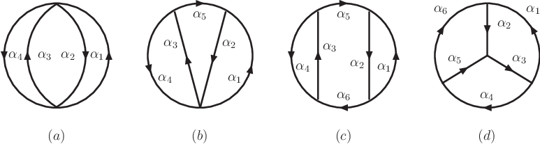
From the derivation of the formulae in the last section, it is clear that one can go to higher loop orders by iteratively applying the duality Eq. (20) to the occurring loops. In Ref. [8], all four scalar master diagrams at three loops are considered as given in Fig. 2 and formulae provided for their results. These results are not unique in the sense that there is some freedom in the choice of propagators for which the directions of momentum flow are changed in doing the various cuts. For diagrams (a) to (c) a result can be derived in a very similar and fast way, while diagram (d), being the only non–planar diagram, is slightly more involved. As expected, it could be confirmed that the final result always consists of cuts, with a multiplicity ranging from the number of loops of the diagram, up to a cut with the multiplicity of the number of loop lines, where each loop line is cut exactly once, which has the effect of generating disconnected graphs.

The extension to higher loop orders above three loops seems straightforward, though more complex topologies might complicate the way of constructing the final results and its overall structure. However, due to the use of Eq. (2), this result should again involve a sum over cuts with multiplicity starting from the number of loops up to the number of loop lines.

6 CONCLUSION AND OUTLOOK

The duality–theorem derived in Ref. [2] has been reformulated in a way, which allows to extend it to higher loop orders. We explained in detail the steps to obtain a duality relation at two loops, considering the two–loop scalar master diagram and shortly discussed its application to the four three–loop master diagrams. Following these examples, this method provides a straightforward prescription to apply it to even higher loop orders.

References

- [1] J. R. Andersen et al. [SM and NLO Multileg Working Group], “The SM and NLO multileg working group: Summary report,” arXiv:1003.1241 [hep-ph].
- [2] S. Catani, T. Gleisberg, F. Krauss, G. Rodrigo and J. C. Winter, “From loops to trees by-passing Feynman’s theorem,” JHEP 0809 (2008) 065 [arXiv:0804.3170 [hep-ph]].
- [3] D. E. Soper, “QCD calculations by numerical integration,” Phys. Rev. Lett. 81 (1998) 2638, “Techniques for QCD calculations by numerical integration,” Phys. Rev. D 62 (2000) 014009; M. Kramer and D. E. Soper, “Next-to-leading order numerical calculations in Coulomb gauge,” Phys. Rev. D 66 (2002) 054017.
- [4] W. Kilian and T. Kleinschmidt, “Numerical Evaluation of Feynman Loop Integrals by Reduction to Tree Graphs,” arXiv:0912.3495 [hep-ph].
- [5] M. Moretti, F. Piccinini and A. D. Polosa, “A Fully Numerical Approach to One-Loop Amplitudes,” arXiv:0802.4171 [hep-ph].
- [6] R. P. Feynman, “Quantum theory of gravitation,” Acta Phys. Polon. 24 (1963) 697.
- [7] R. P. Feynman, Closed Loop And Tree Diagrams, in Magic Without Magic, ed. J. R. Klauder, (Freeman, San Francisco, 1972), p. 355, in Selected papers of Richard Feynman, ed. L. M. Brown (World Scientific, Singapore, 2000) p. 867.
- [8] I. Bierenbaum, S. Catani, P. Draggiotis and G. Rodrigo, “A Tree-Loop Duality Relation at Two Loops and Beyond,” submitted to arXiv:hep-ph