A Low Density Lattice Decoder
via Non-Parametric Belief Propagation

Abstract

The recent work of Sommer, Feder and Shalvi presented a new family of codes called low density lattice codes (LDLC) that can be decoded efficiently and approach the capacity of the AWGN channel. A linear time iterative decoding scheme which is based on a message-passing formulation on a factor graph is given.

In the current work we report our theoretical findings regarding the relation between the LDLC decoder and belief propagation. We show that the LDLC decoder is an instance of non-parametric belief propagation and further connect it to the Gaussian belief propagation algorithm. Our new results enable borrowing knowledge from the non-parametric and Gaussian belief propagation domains into the LDLC domain. Specifically, we give more general convergence conditions for convergence of the LDLC decoder (under the same assumptions of the original LDLC convergence analysis). We discuss how to extend the LDLC decoder from Latin square to full rank, non-square matrices. We propose an efficient construction of sparse generator matrix and its matching decoder. We report preliminary experimental results which show our decoder has comparable symbol to error rate compared to the original LDLC decoder.

I Introduction

Lattice codes provide a continuous-alphabet encoding procedure, in which integer-valued information bits are converted to positions in Euclidean space. Motivated by the success of low-density parity check (LDPC) codes [1], recent work by Sommer et al. [2] presented low density lattice codes (LDLC). Like LDPC codes, a LDLC code has a sparse decoding matrix which can be decoded efficiently using an iterative message-passing algorithm defined over a factor graph. In the original paper, the lattice codes were limited to Latin squares, and some theoretical results were proven for this special case.

The non-parametric belief propagation (NBP) algorithm is an efficient method for approximated inference on continuous graphical models. The NBP algorithm was originally introduced in [3], but has recently been rediscovered independently in several domains, among them compressive sensing [4, 5] and low density lattice decoding [2], demonstrating very good empirical performance in these systems.

In this work, we investigate the theoretical relations between the LDLC decoder and belief propagation, and show it is an instance of the NBP algorithm. This understanding has both theoretical and practical consequences. From the theory point of view we provide a cleaner and more standard derivation of the LDLC update rules, from the graphical models perspective. From the practical side we propose to use the considerable body of research that exists in the NBP domain to allow construction of efficient decoders.

We further propose a new family of LDLC codes as well as a new LDLC decoder based on the NBP algorithm . By utilizing sparse generator matrices rather than the sparse parity check matrices used in the original LDLC work, we can obtain a more efficient encoder and decoder. We introduce the theoretical foundations which are the basis of our new decoder and give preliminary experimental results which show our decoder has comparable performance to the LDLC decoder.

The structure of this paper is as follows. Section II overviews LDLC codes, belief propagation on factor graph and the LDLC decoder algorithm. Section III rederive the original LDLC algorithm using standard graphical models terminology, and shows it is an instance of the NBP algorithm. Section IV presents a new family of LDLC codes as well as our novel decoder. We further discuss the relation to the GaBP algorithm. In Section V we discuss convergence and give more general sufficient conditions for convergence, under the same assumptions used in the original LDLC work. Section VI brings preliminary experimental results of evaluating our NBP decoder vs. the LDLC decoder. We conclude in Section VII.

II Background

II-A Lattices and low-density lattice codes

An $n$-dimensional lattice $\Lambda$ is defined by a generator matrix $G$ of size $n\times n$. The lattice consists of the discrete set of points $x=(x_{1},x_{2},...,x_{n})\in R^{n}$ with $x=Gb$, where $b\in Z^{n}$ is the set of all possible integer vectors.

A low-density lattice code (LDLC) is a lattice with a non-singular generator matrix $G$, for which $H=G^{-1}$ is sparse. It is convenient to assume that $det(H)=1/det(G)=1$. An $(n,d)$ regular LDLC code has an $H$ matrix with constant row and column degree $d$. In a latin square LDLC, the values of the $d$ non-zero coefficients in each row and each column are some permutation of the values $h_{1},h_{2},\cdots,h_{d}$.

We assume a linear channel with additive white Gaussian noise (AWGN). For a vector of integer-valued information $b$ the transmitted codeword is $x=Gb$, where $G$ is the LDLC encoding matrix, and the received observation is $y=x+w$ where $w$ is a vector of i.i.d. AWGN with diagonal covariance $\sigma^{2}I$. The decoding problem is then to estimate $b$ given the observation vector $y$; for the AWGN channel, the MMSE estimator is

$$b^{*}=\arg\mathop{\min}\limits_{b\in\mathbb{Z}^{n}}||y-Gb||^{2}\,.$$ (1)

II-B Factor graphs and belief propagation

Factor graphs provide a convenient mechanism for representing structure among random variables. Suppose a function or distribution $p(x)$ defined on a large set of variables $x=[x_{1},\ldots,x_{n}]$ factors into a collection of smaller functions $p(x)=\prod_{s}f_{s}(x_{s})$, where each $x_{s}$ is a vector composed of a smaller subset of the $x_{i}$. We represent this factorization as a bipartite graph with “factor nodes” $f_{s}$ and “variable nodes” $x_{i}$, where the neighbors $\Gamma_{s}$ of $f_{s}$ are the variables in $x_{s}$, and the neighbors of $x_{i}$ are the factor nodes which have $x_{i}$ as an argument ($f_{s}$ such that $x_{i}$ in $x_{s}$). For compactness, we use subscripts $s,t$ to indicate factor nodes and $i,j$ to indicate variable nodes, and will use $x$ and $x_{s}$ to indicate sets of variables, typically formed into a vector whose entries are the variables $x_{i}$ which are in the set.

The belief propagation (BP) or sum-product algorithm [6] is a popular technique for estimating the marginal probabilities of each of the variables $x_{i}$. BP follows a message-passing formulation, in which at each iteration $\tau$, every variable passes a message (denoted $M_{is}^{\tau}$) to its neighboring factors, and factors to their neighboring variables. These messages are given by the general form,

$$M^{\tau+1}_{is}(x_{i}) =f_{i}(x_{i})\prod_{t\in\Gamma_{i}\setminus s}M^{\tau}_{ti}(x_{i})\,, M^{\tau+1}_{si}(x_{i}) =\int\limits_{x_{s}\setminus x_{i}}f_{s}(x_{s})\prod\limits_{j\in\Gamma_{s}\setminus i}M^{\tau}_{js}(x_{j})\,.$$ (2)

Here we have included a “local factor” $f_{i}(x_{i})$ for each variable, to better parallel our development in the sequel. When the variables $x_{i}$ take on only a finite number of values, the messages may be represented as vectors; the resulting algorithm has proven effective in many coding applications including low-density parity check (LDPC) codes [7]. In keeping with our focus on continuous-alphabet codes, however, we will focus on implementations for continuous-valued random variables.

II-B1 Gaussian Belief Propagation

When the joint distribution $p(x)$ is Gaussian, $p(x)\propto\exp\{-\frac{1}{2}x^{T}Jx+h^{T}x\}$, the BP messages may also be compactly represented in the same form. Here we use the “information form” of the Gaussian distribution, ${\cal N}(x;\mu,\Sigma)={\cal N}^{-1}(h,J)$ where $J=\Sigma^{-1}$ and $h=J\mu$. In this case, the distribution’s factors can always be written in a pairwise form, so that each function involves at most two variables $x_{i}$, $x_{j}$, with $f_{ij}(x_{i},x_{j})=\exp\{-J_{ij}x_{i}x_{j}\}$, $j\neq i$, and $f_{i}(x_{i})=\exp\{-\frac{1}{2}J_{ii}x_{i}^{2}+h_{i}x_{i}\}$.

Gaussian BP (GaBP) then has messages that are also conveniently represented as information-form Gaussian distributions. If $s$ refers to factor $f_{ij}$, we have

$$M^{\tau+1}_{is}(x_{i}) ={\cal N}^{-1}(\beta_{i\setminus j},\alpha_{i\setminus j})\,, \alpha_{i\backslash j} =J_{ii}+\sum_{{k}\in\Gamma_{i}\setminus j}\alpha_{ki}\,, \beta_{i\backslash j} =h_{i}+\sum_{k\in\Gamma_{i}\setminus j}\beta_{ki}\,,$$ (3)

$$M^{\tau+1}_{sj}(x_{j}) ={\cal N}^{-1}(\beta_{ij},\alpha_{ij})\,, \alpha_{ij} =-J_{ij}^{2}\alpha_{i\backslash j}^{-1}\,, \beta_{ij} =-J_{ij}\alpha_{i\backslash j}^{-1}\beta_{i\backslash j}\,.$$ (4)

From the $\alpha$ and $\beta$ values we can compute the estimated marginal distributions, which are Gaussian with mean $\hat{\mu}_{i}=\hat{K}_{i}(h_{i}+\sum_{k\in\Gamma_{i}}\beta_{ki})$ and variance $\hat{K}_{i}=(J_{ii}+\sum_{{k}\in\Gamma_{i}}\alpha_{ki})^{-1}$. It is known that if GaBP converges, it results in the exact MAP estimate $x^{*}$, although the variance estimates $\hat{K}_{i}$ computed by GaBP are only approximations to the correct variances [8].

II-B2 Nonparametric belief propagation

In more general continuous-valued systems, the messages do not have a simple closed form and must be approximated. Nonparametric belief propagation, or NBP, extends the popular class of particle filtering algorithms, which assume variables are related by a Markov chain, to general graphs. In NBP, messages are represented by collections of weighted samples, smoothed by a Gaussian shape–in other words, Gaussian mixtures.

NBP follows the same message update structure of (2). Notably, when the factors are all either Gaussian or mixtures of Gaussians, the messages will remain mixtures of Gaussians as well, since the product or marginalization of any mixture of Gaussians is also a mixture of Gaussians [3]. However, the product of $d$ Gaussian mixtures, each with $N$ components, produces a mixture of $N^{d}$ components; thus every message product creates an exponential increase in the size of the mixture. For this reason, one must approximate the mixture in some way. NBP typically relies on a stochastic sampling process to preserve only high-likelihood components, and a number of sampling algorithms have been designed to ensure that this process is as efficient as possible [9, 10, 11]. One may also apply various deterministic algorithms to reduce the number of Gaussian mixture components [12]; for example, in [13, 14], an $O(N)$ greedy algorithm (where $N$ is the number of components before reduction) is used to trade off representation size with approximation error under various measures.

II-C LDLC decoder

The LDLC decoding algorithm is also described as a message-passing algorithm defined on a factor graph[6], whose factors represent the information and constraints on $x$ arising from our knowledge of $y$ and the fact that $b$ is integer-valued. Here, we rewrite the LDLC decoder update rules in the more standard graphical models notation. The factor graph used is a bipartite graph with variables nodes $\{x_{i}\}$, representing each element of the vector $x$, and factor nodes $\{f_{i},g_{s}\}$ corresponding to functions

$$f_{i}(x_{i}) =\mathcal{N}(x_{i};y_{i},\sigma^{2})\,, g_{s}(x_{s}) =\begin{cases}1&H_{s}x\in\mathbb{Z}\\ 0&\mathrm{otherwise}\end{cases}\,,$$

where $H_{s}$ is the $s^{\mathrm{th}}$ row of the decoding matrix $H$. Each variable node $x_{i}$ is connected to those factors for which it is an argument; since $H$ is sparse, $H_{s}$ has few non-zero entries, making the resulting factor graph sparse as well. Notice that unlike the construction of [2], this formulation does not require that $H$ be square, and it may have arbitrary entries, rather than being restricted to a Latin square construction. Sparsity is preferred, both for computational efficiency and because belief propagation is typically more well behaved on sparse systems with sufficiently long cycles [6]. We can now directly derive the belief propagation update equations as Gaussian mixture distributions, corresponding to an instance of the NBP algorithm. We suppress the iteration number $\tau$ to reduce clutter.

Variable to factor messages. Suppose that our factor to variable messages $M_{si}(x_{i})$ are each described by a Gaussian mixture distribution, which we will write in both the moment and information form:

$$M_{si}(x_{i})=\sum_{l}w_{si}^{l}\mathcal{N}(x_{i}\,;\,m_{si}^{l},\nu_{si}^{l})=\sum_{l}w_{si}^{l}\mathcal{N}^{-1}(x_{i}\,;\,\beta_{si}^{l},\alpha_{si}^{l})\,.$$ (5)

Then, the variable to factor message $M_{is}(x_{s})$ is given by

$$M_{is}(x_{s})=\sum_{l}w_{is}^{l}\mathcal{N}(x_{s}\,;\,m_{is}^{l},\nu_{is}^{l})=\sum_{l}w_{is}^{\mathbf{l}}\mathcal{N}^{-1}(x_{s}\,;\,\beta_{is}^{l},\alpha_{is}^{l})\,,$$ (6)

where ${\mathbf{l}}$ refers to a vector of indices $[{l}_{s}]$ for each neighbor $s$,

$$\alpha_{is}^{{\bf l}} =\sigma^{-2}+\sum_{t\in\Gamma_{i}\setminus s}\alpha_{ti}^{{l}_{t}}\,, \beta_{it}^{\mathbf{l}} =y_{i}\sigma^{-2}+\sum_{t\in\Gamma_{i}\setminus s}\beta_{ti}^{{l}_{s}}\,, w_{it}^{\mathbf{l}} =\frac{\mathcal{N}(x^{*};y_{i},\sigma^{2})\prod w_{si}^{{l}_{s}}\mathcal{N}^{-1}(x^{*};\beta_{si}^{{l}_{s}},\alpha_{si}^{{l}_{s}})}{\mathcal{N}^{-1}(x^{*};\beta_{it}^{\mathbf{l}},\alpha_{it}^{\mathbf{l}})}\,.$$ (7)

The moment parameters are then given by $\nu_{it}^{\mathbf{l}}=(\alpha_{it}^{\mathbf{l}})^{-1}$, $m_{it}^{\mathbf{l}}=\beta_{it}^{\mathbf{l}}(\alpha_{it}^{\mathbf{l}})^{-1}$. The value $x^{*}$ is any arbitrarily chosen point, often taken to be the mean $m_{it}^{\mathbf{l}}$ for numerical reasons.

Factor to variable messages. Assume that the incoming messages are of the form (6), and note that the factor $g_{s}(\cdot)$ can be rewritten in a summation form, $g_{s}(x_{s})=\sum_{b_{s}}\delta(H_{s}x=b_{s})$, which includes all possible integer values $b_{s}$. If we condition on the value of both the integer $b_{s}$ and the indices of the incoming messages, again formed into a vector ${\mathbf{l}}=[{l}_{j}]$ with an element for each variable $j$, we can see that $g_{s}$ enforces the linear equality $H_{si}x_{i}=b_{s}-\sum H_{sj}x_{j}$. Using standard Gaussian identities in the moment parameterization and summing over all possible $b_{s}\in\mathbb{Z}$ and ${\mathbf{l}}$, we obtain

$$M_{si}(x_{i})=\sum_{b_{s}}\sum_{\mathbf{l}}w_{si}^{\mathbf{l}}\mathcal{N}(x_{i}\,;\,m_{si}^{\mathbf{l}},\nu_{si}^{\mathbf{l}})=\sum_{b_{s}}\sum_{\mathbf{l}}w_{si}^{\mathbf{l}}\mathcal{N}^{-1}(x_{i}\,;\,\beta_{si}^{\mathbf{l}},\alpha_{si}^{\mathbf{l}})\,,$$ (8)

where

$$\nu_{si}^{\mathbf{l}} =H_{si}^{-2}\left(\sum_{j\in\Gamma_{s}\setminus i}H_{js}^{2}\nu_{js}^{{l}_{j}}\right)\,, m_{si}^{\mathbf{l}} =H_{si}^{-1}\left(-b_{s}+\sum_{j\in\Gamma_{s}\setminus i}H_{js}m_{js}^{{l}_{j}}\right)\,, w_{si}^{\mathbf{l}} =\prod_{j\in\Gamma_{s}\setminus i}w_{js}^{{l}_{j}}\,,$$ (9)

and the information parameters are given by $\alpha_{si}^{\mathbf{l}}=(\nu_{si}^{\mathbf{l}})^{-1}$ and $\beta_{si}^{\mathbf{l}}=m_{si}^{\mathbf{l}}(\nu_{si}^{\mathbf{l}})^{-1}$.

Notice that (8) matches the initial assumption of a Gaussian mixture given in (5). At each iteration, the exact messages remain mixtures of Gaussians, and the algorithm iteslf corresponds to an instance of NBP. As in any NBP implementation, we also see that the number of components is increasing at each iteration and must eventually approximate the messages using some finite number of components. To date the work on LDLC decoders has focused on deterministic approximations [2, 15, 16, 17], often greedy in nature. However, the existing literature on NBP contains a large number of deterministic and stochastic approximation algorithms [9, 13, 12, 10, 11]. These algorithms can use spatial data structures such as KD-Trees to improve efficiency and avoid the pitfalls that come with greedy optimization.

Estimating the codewords. The original codeword $x$ can be estimated using its belief, an approximation to its marginal distribution given the constraints and observations:

$$B_{i}(x_{i})=f_{i}(x_{i})\prod_{s\in\Gamma_{i}}M_{si}(x_{i})\,.$$ (10)

The value of each $x_{i}$ can then be estimated as either the mean or mode of the belief, e.g., $x_{i}^{*}=\arg\max B_{i}(x_{i})$, and the integer-valued information vector estimated as $b^{*}=\mathop{\mathrm{round}}(Hx^{*})$.

III A Pairwise Construction of the LDLC decoder

Before introducing our novel lattice code construction, we demonstrate that the LDLC decoder can be equivalently constructed using a pairwise graphical model. This construction will have important consequences when relating the LDLC decoder to Gaussian belief propagation (Section IV-B) and understanding convergence properties (Section V).

Theorem 1

The LDLC decoder algorithm is an instance of the NBP algorithm executed on the following pairwise graphical model. Denote the number LDLC variable nodes as $n$ and the number of check nodes as $k$. We construct a new graphical model with $n+k$ variables, $X=(x_{1},\cdots,x_{n+k}$) as follows. To match the LDLC notation we use the index letters $i,j,..$ to denote variables $1,...,n$ and the letters $s,t,...$ to denote new variables $n+1,...,n+k$ which will take the place of the check node factors in the original formulation. We further define the self and edge potentials:

$$\psi_{i}(x_{i}) \propto\mathcal{N}(x_{i};y_{i},\sigma^{2})\,, \psi_{s}(x_{s}) \triangleq\sum_{b_{s}=-\infty}^{\infty}\mathcal{N}^{-1}(x_{s};b_{s},0)\,, \psi_{i,s}(x_{i},x_{s})\triangleq\exp(-x_{i}H_{is}x_{s})\,.$$ (11)

Proof:

The proof is constructed by substituting the edge and self potentials (17) into the belief propagation update rules. Since we are using a pairwise graphical model, we do not have two update rules from variable to factors and from factors to variables. However, to recover the LDLC update rules, we make the artificial distinction between the variable and factor nodes, where the nodes $x_{i}$ will be shown to be related to the variable nodes in the LDLC decoder, and the nodes $x_{s}$ will be shown to be related to the factor nodes in the LDLC decoder.

LDLC variable to factor nodes

We start with the integral-product rule computed in the $x_{i}$ nodes:

$$M_{is}(x_{s})=\int\limits_{x_{i}}\psi(x_{i},x_{s})\psi_{i}(x_{i})\prod_{t\in\Gamma_{i}\setminus s}M_{ti}(x_{i})dx_{i}\,$$

The product of a mixture of Gaussians $\prod\limits_{t\in\Gamma_{i}\setminus s}M_{ti}(x_{i})$ is itself a mixture of Gaussians, where each component in the output mixture is the product of a single Gaussians selected from each input mixture $M_{ti}(x_{i})$.

Lemma 2 (Gaussian product)

[18, Claim 10], [2, Claim 2] Given $p$ Gaussians $\mathcal{N}(m_{1},v_{1}),\cdots,\mathcal{N}(m_{p},v_{p})$ their product is proportional to a Gaussian $\mathcal{N}(\bar{m},\bar{v})$ with

$$\bar{v}^{-1}=\sum_{i=1}^{p}\frac{1}{v_{i}}=\sum_{i=1}^{p}\alpha_{i}\, \bar{m}=(\sum_{i=1}^{p}m_{i}/v_{i})\bar{v}=\sum_{i=1}^{p}\beta_{i}\bar{v}$$

Proof:

Is given in [18, Claim 10]. ∎ Using the Gaussian product lemma the $l_{s}$ mixture component in the message from variable node $i$ to factor node $s$ is a single Gaussian given by

$$M^{l_{s}}_{is}(x_{s})=\int\limits_{x_{i}}\psi_{is}(x_{i},x_{s})\Big(\psi_{i}(x_{i})\prod_{t\in\Gamma_{i}\setminus s}M^{\tau}_{ti}(x_{i})\Big)dx_{i}=$$

$${\int\limits_{x_{i}}}\psi_{is}(x_{i},x_{s})\Big(\psi_{i}(x_{i}){\exp\{{-\tfrac{1}{2}}x_{i}^{2}(\sum_{t\in\Gamma_{i}\setminus s}\alpha_{ti}^{l_{s}})+x_{i}(\sum_{t\in\Gamma_{i}\backslash s}\beta_{ti}^{l_{s}}\,)\}}\Big)dx_{i}=$$

$${\int\limits_{x_{i}}}\psi_{is}(x_{i},x_{s})\Big(\exp(-\tfrac{1}{2}x^{2}\sigma^{-2}+x_{i}y_{i}\sigma^{-2}){\exp\{{-\tfrac{1}{2}}x_{i}^{2}(\sum_{t\in\Gamma_{i}\setminus s}\alpha_{ti}^{l_{s}})+x_{i}(\sum_{t\in\Gamma_{i}\backslash s}\beta_{ti}^{l_{s}}\,)\}}\Big)dx_{i}=$$

$${\int\limits_{x_{i}}}\psi_{is}(x_{i},x_{s})\Big({\exp\{{-\tfrac{1}{2}}x_{i}^{2}(\sigma^{-2}+\sum_{t\in\Gamma_{i}\setminus s}\alpha_{ti}^{l_{s}})+x_{i}(y_{i}\sigma^{-2}+\sum_{t\in\Gamma_{i}\backslash s}\beta_{ti}^{l_{s}}\,)\,\}}\Big)dx_{i}\,.$$

We got a formulation which is equivalent to LDLC variable nodes update rule given in (7). Now we use the following lemma for computing the integral:

Lemma 3 (Gaussian integral)

Given a (one dimensional) Gaussian $\phi_{i}(x_{i})\propto\mathcal{N}(x_{i};m,v)$, the integral $\int\limits_{x_{i}}\psi_{i,s}(x_{i},x_{s})\phi_{i}(x_{i})dx_{i}$ , where is a (two dimensional) Gaussian $\psi_{i,s}(x_{i},x_{s})\triangleq\exp(-\tfrac{}{}x_{i}H_{is}x_{s})$  is proportional to a (one dimensional) Gaussian $\mathcal{N}^{{-1}}(H_{is}m,H_{is}^{2}v).$

Proof:

$$\int\limits_{x_{i}}\psi_{ij}(x_{i},x_{j})\phi_{i}(x_{i})dx_{i}\ \ \ \propto\ \ \ \int\limits_{x_{i}}\exp{(-x_{i}H_{is}x_{s})}{\exp\{{-\tfrac{1}{2}}(x_{i}-m)^{2}/v\}}dx_{i}=$$

$$={\int\limits_{x_{i}}}\exp{\Big((-\tfrac{1}{2}x_{i}^{2}/v)+(m/v-H_{is}x_{s})x_{i}\Big)}dx_{i}\ \ \ \propto\ \ \ \exp{((m/v-H_{is}x_{s})^{2}/(-\tfrac{2}{v}))}\,,$$

where the last transition was obtained by using the Gaussian integral:

$$\int\limits_{-\infty}^{\infty}\exp{(-ax^{2}+bx)}dx=\sqrt{\pi/a}\exp{(b^{2}/4a)}.$$

$$\exp{((m/v-H_{is}x_{s})^{2}/(-\tfrac{2}{v}))}={\exp\{{-\tfrac{1}{2}}(v(m/v-H_{is}x_{s})^{2})\}}=$$

$$={\exp\{{-\tfrac{1}{2}}(H_{is}^{2}v)x_{s}^{2}+(H_{is}m)x_{s}-\tfrac{1}{2}v(m/v)^{2}\}}\propto{\exp\{{-\tfrac{1}{2}}(H_{is}^{2}v)x_{s}^{2}+(H_{is}m)x_{s}\}}\,.$$

∎ Using the results of Lemma 3 we get that the sent message between variable node to a factor node is a mixture of Gaussians, where each Gaussian component $k$ is given by

$$M^{{\mathbf{l}}}_{is}(x_{s})=\mathcal{N}^{-1}(x_{s};H_{is}m_{is}^{l_{s}},H^{2}_{is}v_{is}^{l_{s}})\,.$$

Note that in the LDLC terminology the integral operation as defined in Lemma 3 is called stretching. In the LDLC algorithm, the stretching is computed by the factor node as it receives the message from the variable node. In NBP, the integral operation is computed at the variable nodes.

LDLC Factors to variable nodes

We start again with the BP integral-product rule and handle the $x_{s}$ variables computed at the factor nodes.

$$M_{si}(x_{i})=\int\limits_{x_{s}}\psi_{is}(x_{i},x_{s})\psi_{s}(x_{s})\prod\limits_{j\in\Gamma_{s}\setminus i}M_{js}(x_{j})\,dx_{s}.$$

Note that the product $\prod\limits_{j\in\Gamma_{s}\setminus i}M^{\tau}_{js}(x_{j})$ is a mixture of Gaussians, where the $k$-th component is computed by selecting a single Gaussian from each message $M^{\tau}_{js}$ from the set $j\in\Gamma_{s}\setminus i$ and applying the product lemma (Lemma 2). We get

$${\int\limits_{x_{s}}}\psi_{is}(x_{i},x_{s})\Big(\psi_{s}(x_{s}){\exp\{{-\tfrac{1}{2}}x_{s}^{2}(\sum_{k\in\Gamma_{s}\backslash i}H^{2}_{ks}v_{ks}^{l_{i}})+x_{s}(\sum_{k\in\Gamma_{s}\setminus i}H_{ks}m_{ks}^{l_{i}})\,\}}\Big)dx_{s}$$ (12)

We continue by computing the product with the self potential $\psi_{s}(x_{s})$ to get

$$={\int\limits_{x_{s}}}\psi_{is}(x_{i},x_{s})\Big(\sum_{b_{s}=-\infty}^{\infty}\exp(b_{s}x_{s}){\exp\{{-\tfrac{1}{2}}x_{s}^{2}(\sum_{k\in\Gamma_{s}\backslash i}H^{2}_{ks}v_{ks}^{l_{i}})+x_{s}(\sum_{k\in\Gamma_{s}\setminus i}H_{ks}m_{ks}^{l_{i}})\,\}}\Big)dx_{s}=$$

$$=\sum_{b_{s}=-\infty}^{\infty}{\int\limits_{x_{s}}}\psi_{is}(x_{i},x_{s})\Big(\exp(b_{s}x_{s}){\exp\{{-\tfrac{1}{2}}x_{s}^{2}(\sum_{k\in\Gamma_{s}\backslash i}H^{2}_{ks}v_{ks}^{l_{i}})+x_{s}(\sum_{k\in\Gamma_{s}\setminus i}H_{ks}m_{ks}^{l_{i}})\,\}}\Big)dx_{s}=$$

$$=\sum_{b_{s}=-\infty}^{\infty}{\int\limits_{x_{s}}}\psi_{is}(x_{i},x_{s})\Big({\exp\{{-\tfrac{1}{2}}x_{s}^{2}(\sum_{k\in\Gamma_{s}\backslash i}H^{2}_{ks}v_{ks}^{l_{i}})+x_{s}(b_{s}+\sum_{k\in\Gamma_{s}\setminus i}H_{ks}m_{ks}^{l_{i}})\,\}}\Big)dx_{s}=$$

$$=\sum_{b_{s}=\infty}^{-\infty}{\int\limits_{x_{s}}}\psi_{is}(x_{i},x_{s})\Big({\exp\{{-\tfrac{1}{2}}x_{s}^{2}(\sum_{k\in\Gamma_{s}\backslash i}H^{2}_{ks}v_{ks}^{l_{i}})+x_{s}(-b_{s}+\sum_{k\in\Gamma_{s}\setminus i}H_{ks}m_{ks}^{l_{i}})\,\}}\Big)dx_{s}\,.$$

Finally we use Lemma 3 to compute the integral and get

$$=\sum_{b_{s}=\infty}^{-\infty}{\exp\{{-\tfrac{1}{2}}x_{s}^{2}H_{si}^{2}(\sum_{k\in\Gamma_{s}\backslash i}H^{2}_{ks}v_{ks}^{l_{i}})^{-1}+x_{s}H_{si}(\sum_{k\in\Gamma_{s}\backslash i}H^{2}_{ks}v_{ks}^{l_{i}})^{-1}(-b_{s}+\sum_{k\in\Gamma_{s}\setminus i}H_{ks}m_{ks}^{l_{i}})\,\}}dx_{s}\,.$$

It is easy to verify this formulation is identical to the LDLC update rules (9). ∎

IV Using Sparse Generator Matrices

We propose a new family of LDLC codes where the generator matrix $G$ is sparse, in contrast to the original LDLC codes where the parity check matrix $H$ is sparse. Table I outlines the properties of our proposed decoder. Our decoder is designed to be more efficient than the original LDLC decoder, since as we will soon show, both encoding, decoding and initialization operations are more efficient in the NBP decoder. We are currently in the process of fully evaluating our decoder performance relative to the LDLC decoder. Initial results are reported in Section VI. Our decoder is available for download on [19].

IV-A The NBP decoder

We use an undirected bipartite graph, with variables nodes $\{b_{i}\}$, representing each element of the vector $b$, and observation nodes $\{z_{i}\}$ for each element of the observation vector $y$. We define the self potentials $\psi_{i}(z_{i})$ and $\psi_{s}(b_{s})$ as follows:

$$\psi_{i}(z_{i}) \propto\mathcal{N}(z_{i};y_{i},\sigma^{2})\,, \psi_{s}(b_{s}) =\begin{cases}1&b_{s}\in\mathbb{Z}\\ 0&\mathrm{otherwise}\end{cases}\,,$$ (13)

and the edge potentials:

$$\psi_{i,s}(z_{i},b_{s})\triangleq\exp(-\tfrac{1}{2}z_{i}G_{is}x_{s})\,.$$

Each variable node $b_{s}$ is connected to the observation nodes as defined by the encoding matrix $G.$ Since $G$ is sparse, the resulting bipartite graph sparse as well. As with LDPC decoders [7], the belief propagation or sum-product algorithm [20, 6] provides a powerful approximate decoding scheme.

For computing the MAP assignment of the transmitted vector $b$ using non-parametric belief propagation we perform the following relaxation, which is one of the main novel contributions of this paper. Recall that in the original problem, $b$ are only allowed to be integers. We relax the function $\psi_{s}(x_{s})$ from a delta function to a mixture of Gaussians centered around integers.

$$\psi^{relax}_{s}(b_{s})\propto\sum_{i\in\mathbb{Z}}\mathcal{N}(i,v)\,.$$

Fig. 1: The approximating function $g^{relax}_{s}(x)$ for the binary case.

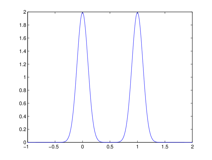
The variance parameter $v$ controls the approximation quality, as $v\rightarrow 0$ the approximation quality is higher. Figure 2 plots an example relaxation of $\psi_{i}(b_{s})$ in the binary case. We have defined the self and edge potentials which are the input the to the NBP algorithm. Now it is possible to run the NBP algorithm using (2) and get an approximate MAP solution to (1). The derivation of the NBP decoder update rules is similar to the one done for the LDLC decoder, thus omitted. However, there are several important differences that should be addressed. We start by analyzing the algorithm efficiency.

Algorithm	LDLC	NBP
Initialization operation	$G=H^{-1}$	None
Initialization cost	$O(n^{3})$	-
Encoding operation	$Gb$	$Gb$
Encoding cost	$O(n^{2})$	$O(nd),\ \ \ d\ll n$
Cost per node per iteration	$O(q\log(q)d)$	$O(qd)$
Post run operation	$Hx$	None
Post run cost	$O(nd)$	-

TABLE I: Comparison of LDLC decoder vs. NBP decoder

We assume that the input to our decoder is the sparse matrix $G$, there is no need in computing the encoding matrix $G=H^{-1}$ as done in the LDLC decoder. Naively this initialization takes $O(n^{3})$ cost. The encoding in our scheme is done as in LDLC by computing the multiplication $Gb$. However, since $G$ is sparse in our case, encoding cost is $O(nd)$ where $d<<n$ is the average number of non-zeros entries on each row. Encoding in the LDLC method is done in $O(n^{2})$ since even if $H$ is sparse, $G$ is typically dense. After convergence, the LDLC decoder multiplies by the matrix $H$ and rounds the result to get $b$. This operation costs $O(nd)$ where $d$ is the average number of non-zero entries in $H$. In contrast, in the NBP decoder, $b$ is computed directly in the variable nodes.

Besides of efficiency, there are several inherent differences between the two algorithms. Summary of the differences is given in Table II. First, we use a standard formulation of BP using pairwise potentials form, which means there is a single update rule, and not two update rules from left to right and right to left. This can potentially allow more efficient implementations, since the LDLC decoder can be implemented using quantization, such that the convolution is computed in the fft domain. In our framework, there is no convolution, and they product using quantization is computed using elementwise product. Second, our formulation is different since we use different self potentials. The self potentials are incorporated into the computation via the product rule of the integral-product algorithm. Our self potentials perform operations which are equivalent in the LDLC terminology to the convolution and periodic extension operation. The integral computed in the NBP decoder is related to the stretch/unstretch operation of the LDLC decoder.

Algorithm	LDLC decoder	NBP decoder
Update rules	Two: factor to variables and vice versa	One
Sparsity assumption	Decoding matrix H	Encoding matrix G
Algorithm derivation	Custom	Standard NBP
Graphical model	Factor graph	Pairwise potentials
Related Operations	Stretch/Unstretch	Integral
	Convolution	product
	periodic extension	product

TABLE II: Inheret differences between LDLC and NBP decoders

IV-B The relation of the NBP decoder to GaBP

In this section we show that simplified version of the NBP decoder coincides with the GaBP algorithm. The simplified version is obtained, when instead of using our proposed Gaussian mixture prior, we initialize the NBP algorithm with a prior composed of a single Gaussian.

Theorem 4

By initializing $\psi_{s}(b_{s})\sim\mathcal{N}(0,1)$ to be a (single) Gaussian the NBP decoder update rules are identical to update rules of the GaBP algorithm.

Lemma 5

By initializing $\psi_{s}(x_{s})$ to be a (single) Gaussian the messages of the NBP decoder are single Gaussians.

Proof:

Assume both the self potentials $\psi_{s}(b_{s}),\psi_{i}(z_{i})$ are initialized to a single Gaussian, every message of the NBP decoder algorithm will remain a Gaussian. This is because the product (3) of single Gaussians is a single Gaussian, the integral and (4) of single Gaussians produce a single Gaussian as well. ∎Now we are able to prove Theorem 4:

Proof:

We start writing the update rules of the variable nodes. We initialize the self potentials of the variable nodes $\psi_{i}(z_{i})=\mathcal{N}(z_{i};y_{i},\sigma^{2})\,$, Now we substitute, using the product lemma and Lemma 3.

$$M_{is}(b_{s})=\int\limits_{z_{i}}\psi_{i,s}(z_{i},b_{s})\Big(\psi_{i}(z_{i})\prod\limits_{t\in\Gamma_{i}\setminus s}M_{ti}(z_{i})\Big)dz_{i}=$$

$${\int\limits_{z_{i}}}\psi_{i,s}(z_{i},b_{s})\Big(\exp(-\tfrac{1}{2}z_{i}^{2}\sigma^{-2}+y_{i}z_{i}\sigma^{-2})\prod\limits_{t\in\Gamma_{i}\setminus s}\exp(-\tfrac{1}{2}z_{i}^{2}\alpha_{ti}+z_{i}\beta_{ti})\Big)dz_{i}$$

$${\int\limits_{z_{i}}}\psi_{i,s}(z_{i},b_{s})\Big(\exp(-\tfrac{1}{2}z_{i}^{2}(\sigma^{-2}+\sum_{t\in\Gamma_{i}\setminus s}\alpha_{ti})+z_{i}(\sigma^{-2}y_{i}+\sum_{t\in\Gamma_{i}\setminus s}\beta_{ti})\Big)dz_{i}=$$

$$\propto\exp\Big(-\tfrac{1}{2}z_{i}^{2}G^{2}_{is}(\sigma^{-2}+\sum_{t\in\Gamma_{i}\setminus s}\alpha_{ti})^{-1}+z_{i}G_{is}(\sigma^{-2}+\sum_{t\in\Gamma_{i}\setminus s}\alpha_{ti})^{-1}(\sigma^{-2}y_{i}+\sum_{t\in\Gamma_{i}\setminus s}\beta_{ti})\Big)$$

Now we get GaBP update rules by substituting $J_{ii}\triangleq\sigma^{-2},J_{is}\triangleq G_{is},h_{s}\triangleq\sigma^{-2}y_{i}:$

$${\alpha_{is}=-J_{is}^{2}\alpha_{i\setminus s}^{-1}=-J_{is}^{2}(J_{ii}+\sum\limits_{{t}\in\Gamma_{i}\setminus s}\alpha_{ti})^{-1}}, {\beta_{is}=-J_{is}\alpha_{i\setminus s}^{-1}\beta_{i\setminus s}=-J_{is}\Big(\alpha_{i\setminus s}^{-1}(h_{i}+\sum\limits_{t\in\Gamma_{i}\setminus s}\beta_{ti})\Big)}\,.$$ (14)

We continue expanding

$$M_{si}(z_{i})=\int\limits_{b_{s}}\psi_{i,s}(z_{i},b_{s})\Big(\psi_{s}(b_{s})\prod\limits_{k\in\Gamma_{s}\backslash i}M^{\tau}_{ks}(b_{s})\Big)db_{s}$$

Similarly using the initializations $\psi_{s}(b_{s})={\exp\{{-\tfrac{1}{2}}b_{s}^{2}\}},\ \psi_{i,s}(z_{i},b_{s})\triangleq\exp(-z_{i}G_{is}b_{s}).$

$${\int\limits_{b_{s}}}\psi_{i,s}(z_{i},b_{s})\Big({\exp\{{-\tfrac{1}{2}}b_{s}^{2}\}}\prod\limits_{k\in\Gamma_{s}\backslash i}\exp(-\tfrac{1}{2}b_{s}^{2}\alpha_{is}+b_{s}\beta_{ks})\Big)db_{s}=$$

$${\int\limits_{b_{s}}}\psi_{i,s}(z_{i},b_{s})\Big({\exp\{{-\tfrac{1}{2}}b_{s}^{2}(1+\sum\limits_{k\in\Gamma_{s}\backslash i}\alpha_{is})+b_{s}(\sum\limits_{k\in\Gamma_{s}\backslash i}\beta_{ks})\}}\Big)db_{s}=$$

$${\exp\{{-\tfrac{1}{2}}b_{s}^{2}G_{is}^{2}(1+\sum\limits_{k\in\Gamma_{s}\backslash i}\alpha_{is})^{-1}+b_{s}G_{is}(1+\sum\limits_{k\in\Gamma_{s}\backslash i}\alpha_{is})^{-1}(\sum\limits_{k\in\Gamma_{s}\backslash i}\beta_{ks})\}}$$

Now we get GaBP update rules by substituting $J_{ii}\triangleq 1,J_{si}\triangleq G_{is},h_{i}\triangleq 0:$

$${\alpha_{si}=-J_{si}^{2}\alpha_{s\setminus i}^{-1}=-J_{si}^{2}(J_{ii}+\sum\limits_{{k}\in\Gamma s\setminus i}\alpha_{is})^{-1}}, {\beta_{si}=-J_{si}\alpha_{s\setminus i}^{-1}\beta_{s\setminus i}=-J_{si}\Big(\alpha_{s\setminus i}^{-1}(h_{i}+\sum\limits_{{k}\in\Gamma s\setminus i}\beta_{ks})\Big)}\,.$$ (15)

∎ Tying together the results, in the case of a single Gaussian self potential, the NBP decoder is initialized using the following inverse covariance matrix:

$$J\triangleq\begin{pmatrix}I&G\\ G^{T}&\ \mathop{\bf diag}(\sigma^{-2})\end{pmatrix}$$

We have shown that a simpler version of the NBP decoder, when the self potentials are initialized to be single Gaussians boils down to GaBP algorithm. It is known [21] that the GaBP algorithm solves the following least square problem $\min_{b\in\mathbb{R}^{n}}\|Gb-y\|$ assuming a Gaussian prior on $b$, $p(b)\sim\mathcal{N}(0,1)$, we get the MMSE solution $b^{*}=(G^{T}G)^{-1}G^{T}y.$ Note the relation to (1). The difference is that we relax the LDLC decoder assumption that $b\in\mathbb{Z}^{n}$, with $b\in\mathbb{R}^{n}$.

Getting back to the NBP decoder, Figure 2 compares the two different priors used, in the NBP decoder and in the GaBP algorithm, for the bipolar case where $b\in\{-1,1\}$. It is clear that the Gaussian prior assumption on $b$ is not accurate enough. In the NBP decoder, we relax the delta function (13) to a Gaussian mixture prior composed of mixtures centered around Integers. Overall, the NBP decoder algorithm can be thought of as an extension of the GaBP algorithm with more accurate priors.

Fig. 2: Comparing GaBP prior to the prior we use in the NBP decoder for the bipolar case $(b\in\{-1,1\}$).

V Convergence analysis

The behavior of the belief propagation algorithm has been extensively studied in the literature, resulting in sufficient conditions for convergence in the discrete case [22] and in jointly Gaussian models [23]. However, little is known about the behavior of BP in more general continuous systems. The original LDLC paper [2] gives some characterization of its convergence properties under several simplifying assumptions. Relaxing some of these assumptions and using our pairwise factor formulation, we show that the conditions for GaBP convergence can also be applied to yield new convergence properties for the LDLC decoder.

The most important assumption made in the LDLC convergence analysis [2] is that the system converges to a set of “consistent” Gaussians; specifically, that at all iterations $\tau$ beyond some number $\tau_{0}$, only a single integer $b_{s}$ contributes to the Gaussian mixture. Notionally, this corresponds to the idea that the decoded information values themselves are well resolved, and the convergence being analyzed is with respect to the transmitted bits $x_{i}$. Under this (potentially strong) assumption, sufficient conditions are given for the decoder’s convergence. The authors also assume that $H$ consists of a Latin square in which each row and column contain some permutation of the scalar values $h_{1}\geq\ldots\geq h_{d}$, up to an arbitrary sign.

Four conditions are given which should all hold to ensure convergence:

• LDLC-I: $\det(H)=\det(G)=1$.

• LDLC-II: $\alpha\leq 1$, where $\alpha\triangleq\frac{\sum_{i=2}^{d}h^{2}_{i}}{h^{2}_{1}}$.

• LDLC-III: The spectral radius of $\rho(F)<1$ where $F$ is a $n\times n$ matrix defined by:

  $$F_{k,l}=\begin{cases}\frac{h_{rk}}{h_{r}l}&\mbox{if $k\neq l$ and there exist a row $r$ of $H$ for which $|H_{rl}|=h_{1}$ and $H_{rk}\neq 0$}\\ 0&\mbox{otherwise}\\ \end{cases}$$

• LDLC-IV: The spectral radius of $\rho(\tilde{H})<1$ where $\tilde{H}$ is derived from H by permuting the rows such that the $h_{1}$ elements will be placed on the diagonal, dividing each row by the appropriate diagonal element ($+h_{1}$ or $-h_{1}$), and then nullifying the diagonal.

Using our new results we are now able to provide new convergence conditions for the LDLC decoder.

Corollary 6

The convergence of the LDLC decoder depends on the properties of the following matrix:

$$J\triangleq\begin{pmatrix}{\mathbf{0}}&H\\ H^{T}&\ \mathop{\bf diag}(1/\sigma^{2})\end{pmatrix}$$ (16)

Proof:

In Theorem 1 we have shown an equivalence between the LDLC algorithm to NBP initialized with the following potentials:

$$\psi_{i}(x_{i}) \propto\mathcal{N}(x_{i};y_{i},\sigma^{2})\,, \psi_{s}(x_{s}) \triangleq\sum_{b_{s}=-\infty}^{\infty}\mathcal{N}^{-1}(x_{s};b_{s},0)\,, \psi_{i,s}(x_{i},x_{s})\triangleq\exp(x_{i}H_{is}x_{s})\,.$$ (17)

We have further discussed the relation between the self potential $\psi_{s}(x_{s})$ and the periodic extension operation. We have also shown in Theorem 4 that if $\psi_{s}(x_{s})$ is a single Gaussian (equivalent to the assumption of “consistent” behavior), the distribution is jointly Gaussian and rather than NBP (with Gaussian mixture messages), we obtain GaBP (with Gaussian messages). Convergence of the GaBP algorithm is dependent on the inverse covariance matrix $J$ and not on the shift vector $h$.

Now we are able to construct the appropriate inverse covariance matrix $J$ based on the pairwise factors given in Theorem 1. The matrix $J$ is a $2\times 2$ block matrix, where the check variables $x_{s}$ are assigned the upper rows and the original variables are assigned the lower rows. The entries can be read out from the quadratic terms of the potentials (17), with the only non-zero entries corresponding to the pairs $(x_{i},x_{s})$ and self potentials $(x_{i},x_{i})$.

∎

Based on Corollary 6 we can characterize the convergence of the LDLC decoder, using the sufficient conditions for convergence of GaBP. Either one of the following two conditions are sufficient for convergence:

• [GaBP-I] (walk-summability [23]) $\rho(I-|D^{-1/2}JD^{-1/2}|)<1$ where $D\triangleq\mathop{\bf diag}(J)$.

• [GaBP-II] (diagonal dominance [8]) $J$ is diagonally dominant (i.e. $|J_{ii}|>=\sum_{j\neq i}|J_{ij}|,\forall i$).

A further difficulty arises from the fact that the upper diagonal of (16) is zero, which means that both [GaBP-I,II] fail to hold. There are three possible ways to overcome this.

1. Create an approximation to the original problem by setting the upper left block matrix of (16) to $\mathop{\bf diag}(\epsilon)$ where $\epsilon>0$ is a small constant. The accuracy of the approximation grows as $\epsilon$ is smaller. In case either of [GaBP-I,II] holds on the fixed matrix the “consistent Gaussians” converge into an approximated solution.

2. In case a permutation on $J$ (16) exists where either [GaBPI,II] hold for permuted matrix, then the “consistent Gaussians” convergence to the correct solution.

3. Use preconditioning to create a new graphical model where the edge potentials are determined by the information matrix $HH^{T}$, $\psi_{i,s}(x_{i},x_{s})\triangleq\exp(x_{i}\{HH^{T}\}_{is}x_{s})$ and the self potentials of the $x_{i}$ nodes are $\psi_{i}(x_{i})\triangleq{\exp\{{-\tfrac{1}{2}}x_{i}^{2}\sigma^{-2}+x_{i}\{Hy\}_{i}\}}$. The proof of the correctness of the above construction is given in [24]. The benefit of this preconditioning is that the main diagonal of $HH^{T}$ is surely non zero. If either [GaBP-I,II] holds on $HH^{T}$ then “consistent Gaussians” convergence to the correct solution. However, the matrix $HH^{T}$ may not be sparse anymore, thus we pay in decoder efficiency.

Overall, we have given two sufficient conditions for convergence, under the “consistent Gaussian” assumption for the means and variances of the LDLC decoder. Our conditions are more general because of two reasons. First, we present a single sufficient condition instead of four that have to hold concurrently in the original LDLC work. Second, our convergence analysis does not assume Latin squares, not even square matrices and does not assume nothing about the sparsity of $H$. This extends the applicability of the LDLC decoder to other types of codes. Note that our convergence analysis relates to the mean and variances of the Gaussian mixture messages. A remaining open problem is the convergence of the amplitudes – the relative heights of the different consistent Gaussians.

VI Experimental results

In this section we report preliminary experimental results of our NBP-based decoder. Our implementation is general and not restricted to the LDLC domain. Specifically, recent work by Baron et al.   [5] had extensively tested our NBP implementation in the context of the related compressive sensing domain. Our Matlab code is available on the web on [19].

We have used a code lengths of $n=100,n=1000$, where the number of non zeros in each row and each column is $d=3$. The non-zeros entries of the sparse encoding matrix $G$ were selected randomly out of $\{-1,1\}$. We have used bipolar signaling, $b\in\{-1,1\}$. We have calculated the maximal noise level $\sigma^{2}_{max}$ using Poltyrov generalized definition for channel capacity using unrestricted power assumption [25]. For bipolar signaling $\sigma^{2}_{max}=4\sqrt[n]{\det(G)^{2}}/2\pi e$. When applied to lattices, the generalized capacity implies that there exists a lattice $G$ of high enough dimension $n$ that enables transmission with arbitrary small error probability, if and only if $\sigma^{2}<\sigma^{2}_{max}$. Figure 3 plots SER (symbol error rate) of the NBP decoder vs. the LDLC decoder for code length $n=100,n=1000$. The $x$-axis represent the distance from capacity in dB as calculated using Poltyrov equation. As can be seen, our novel NBP decoder has better SER for $n=100$ for all noise levels. For $n=1000$ we have better performance for high noise level, and comparable performance up to 0.3dB from LDLC for low noise levels. We are currently in the process of extending our implementation to support code lengths of up $n=100,000$. Initial performance results are very promising.

Fig. 3: NBP vs. LDLC decoder performance

VII Future work and open problems

We have shown that the LDLC decoder is a variant of the NBP algorithm. This allowed us to use current research results from the non-parametric belief propagation domain, to extend the decoder applicability in several directions. First, we have extended algorithm applicability from Latin squares to full column rank matrices (possibly non-square). Second, We have extended the LDLC convergence analysis, by discovering simpler conditions for convergence. Third, we have presented a new family of LDLC which are based on sparse encoding matrices.

We are currently working on an open source implementation of the NBP based decoder, using an undirected graphical model, including a complete comparison of performance to the LDLC decoder. Another area of future work is to examine the practical performance of the efficient Gaussian mixture product sampling algorithms developed in the NBP domain to be applied for LDLC decoder. As little is known about the convergence of the NBP algorithm, we plan to continue examine its convergence in different settings. Finally, we plan to investigate the applicability of the recent convergence fix algorithm [26] for supporting decoding matrices where the sufficient conditions for convergence do not hold.

References

- [1] R. G. Gallager, “Low density parity check codes,” IRE Trans. Inform. Theory, vol. 8, pp. 21–28, 1962.
- [2] N. Sommer, M. Feder, and O. Shalvi, “Low-density lattice codes,” in IEEE Transactions on Information Theory, vol. 54, no. 4, 2008, pp. 1561–1585.
- [3] E. Sudderth, A. Ihler, W. Freeman, and A. Willsky, “Nonparametric belief propagation,” in Conference on Computer Vision and Pattern Recognition (CVPR), June 2003.
- [4] S. Sarvotham, D. Baron, and R. G. Baraniuk, “Compressed sensing reconstruction via belief propagation,” Rice University, Houston, TX, Tech. Rep. TREE0601, July 2006.
- [5] D. Baron, S. Sarvotham, and R. G. Baraniuk, “Bayesian compressive sensing via belief propagation,” IEEE Trans. Signal Processing, to appear, 2009.
- [6] F. Kschischang, B. Frey, and H. A. Loeliger, “Factor graphs and the sum-product algorithm,” vol. 47, pp. 498–519, Feb. 2001.
- [7] R. J. McEliece, D. J. C. MacKay, and J. F. Cheng, “Turbo decoding as an instance of Pearl’s ’belief propagation’ algorithm,” vol. 16, pp. 140–152, Feb. 1998.
- [8] Y. Weiss and W. T. Freeman, “Correctness of belief propagation in Gaussian graphical models of arbitrary topology,” Neural Computation, vol. 13, no. 10, pp. 2173–2200, 2001.
- [9] A. Ihler, E. Sudderth, W. Freeman, and A. Willsky, “Efficient multiscale sampling from products of gaussian mixtures,” in Neural Information Processing Systems (NIPS), Dec. 2003.
- [10] M. Briers, A. Doucet, and S. S. Singh, “Sequential auxiliary particle belief propagation,” in International Conference on Information Fusion, 2005, pp. 705–711.
- [11] D. Rudoy and P. J. Wolf, “Multi-scale MCMC methods for sampling from products of Gaussian mixtures,” in IEEE International Conference on Acoustics, Speech and Signal Processing, vol. 3, 2007, pp. III–1201–III–1204.
- [12] A. T. Ihler. Kernel Density Estimation Toolbox for MATLAB [online] http://www.ics.uci.edu/ihler/code/.
- [13] A. T. Ihler, Fisher, R. L. Moses, and A. S. Willsky, “Nonparametric belief propagation for self-localization of sensor networks,” Selected Areas in Communications, IEEE Journal on, vol. 23, no. 4, pp. 809–819, 2005.
- [14] A. T. Ihler, J. W. Fisher, and A. S. Willsky, “Particle filtering under communications constraints,” in Statistical Signal Processing, 2005 IEEE/SP 13th Workshop on, 2005, pp. 89–94.
- [15] B. Kurkoski and J. Dauwels, “Message-passing decoding of lattices using Gaussian mixtures,” in IEEE Int. Symp. on Inform. Theory (ISIT), Toronto, Canada, July 2008.
- [16] Y. Yona and M. Feder, “Efficient parametric decoder of low density lattice codes,” in IEEE International Symposium on Information Theory (ISIT), Seoul, S. Korea, July 2009.
- [17] B. M. Kurkoski, K. Yamaguchi, and K. Kobayashi, “Single-Gaussian messages and noise thresholds for decoding low-density lattice codes,” in IEEE International Symposium on Information Theory (ISIT), Seoul, S. Korea, July 2009.
- [18] D. Bickson, “Gaussian belief propagation: Theory and application,” Ph.D. dissertation, The Hebrew University of Jerusalem, October 2008.
- [19] Gaussian Belief Propagation implementation in matlab [online] http://www.cs.huji.ac.il/labs/danss/p2p/gabp/.
- [20] J. Pearl, Probabilistic Reasoning in Intelligent Systems: Networks of Plausible Inference. San Francisco: Morgan Kaufmann, 1988.
- [21] O. Shental, D. Bickson, P. H. Siegel, J. K. Wolf, and D. Dolev, “Gaussian belief propagation solver for systems of linear equations,” in IEEE International Symposium on Information Theory (ISIT), Toronto, Canada, July 2008.
- [22] A. T. Ihler, J. W. F. III, and A. S. Willsky, “Loopy belief propagation: Convergence and effects of message errors,” Journal of Machine Learning Research, vol. 6, pp. 905–936, May 2005.
- [23] D. M. Malioutov, J. K. Johnson, and A. S. Willsky, “Walk-sums and belief propagation in Gaussian graphical models,” Journal of Machine Learning Research, vol. 7, Oct. 2006.
- [24] D. Bickson, O. Shental, P. H. Siegel, J. K. Wolf, and D. Dolev, “Gaussian belief propagation based multiuser detection,” in IEEE International Symposium on Information Theory (ISIT), Toronto, Canada, July 2008.
- [25] G. Poltyrev, “On coding without restrictions for the AWGN channel,” in IEEE Trans. Inform. Theory, vol. 40, Mar. 1994, pp. 409–417.
- [26] J. K. Johnson, D. Bickson, and D. Dolev, “Fixing convergence of Gaussian belief propagation,” in IEEE International Symposium on Information Theory (ISIT), Seoul, South Korea, 2009.