Statistical techniques in cosmology

1 Introduction

In these four lectures I cover a number of topics in cosmological data analysis. I concentrate on general techniques which are common in cosmology, or techniques which have been developed in a cosmological context. In fact they have very general applicability, for problems which are firmly model-based, and thus lend themselves to a Bayesian treatment.

We consider the general problem of estimating parameters from data, and consider how one can use Fisher matrices to analyse survey designs before any data are taken, to see whether the survey will actually do what is required. We outline numerical methods for estimating parameters from data, including Monte Carlo Markov Chains and the Hamiltonian Monte Carlo method. We also look at Model Selection, which covers various scenarios such as whether an extra parameter is preferred by the data, or answering wider questions such as which theoretical framework is favoured, using General Relativity and braneworld gravity as an example. These notes are not a literature review, so there are relatively few references. Some of the derivations follow the excellent notes of Licia Verde [24] and Andrew Hamilton [8].

After this introduction, the sections are:

• Parameter Estimation

• Fisher Matrix analysis

• Numerical methods for Parameter Estimation

• Model Selection

Notations:

• Data will be called ${\bf x}$, or $x$, or $x_{i}$, and is written as a vector, even if it is a 2D image.

• Model parameters will be called `, or $\theta$ or $\theta_{\alpha}$

1.1 Inverse problems

Most data analysis problems are inverse problems. You have a set of data ${\vec{x}}$, and you wish to interpret the data in some way. Typical classifications are:

• Hypothesis testing

• Parameter estimation

• Model selection

Cosmological examples of the first type include

• Are CMB data consistent with the hypothesis that the initial fluctuations were gaussian, as predicted by inflation theory?

• Are large-scale structure observations consistent with the hypothesis that the Universe is spatially flat?

Cosmological examples of the second type include

• In the Big Bang model, what is the value of the matter density parameter?

• What is the value of the Hubble constant?

Model selection can include slightly different types (but are mostly concerned with larger, often more qualitative questions):

• Do cosmological data favour the Big Bang theory or the Steady State theory?

• Is the gravity law General Relativity or higher-dimensional?

• Is there evidence for a non-flat Universe?

Note that the notion of a model can be a completely different paradigm (the first two examples), or basically the same model, but with a different parameter set. In the third example, we are comparing a flat Big Bang model with a non-flat one. The latter has an additional parameter, and is considered to be a different model. Similar problems exist elsewhere in astrophysics, such as how many absorption-line systems are required to account for an observed feature?

These lectures will principally be concerned with questions of the last two types, parameter estimation and model selection, but will also touch on experimental design and error forecasting. Hypothesis testing can be treated in a similar manner.

2 Parameter estimation

We collect some data, and wish to interpret them in terms of a model. A model is a theoretical framework which we assume is true. It will typically have some parameters ` in it, which you want to determine. The goal of parameter estimation is to provide estimates of the parameters, and their errors, or ideally the whole probability distribution of `, given the data → x . This is called the posterior probability distribution i.e. it is the probability that the parameter takes certain values, after doing the experiment (as well as assuming a lot of other things):

$$p(\hbox{\bfmath\char 18\relax}|{\vec{x}}).$$ (1)

This is an example of RULE 1: Start by thinking about what it is you want to know, and write it down mathematically.

From $p(\hbox{\bfmath\char 18\relax}|{\vec{x}})$ one can calculate the expectation values of the parameters, and their errors.

2.1 Forward modelling

Often, what may be easily calculable is not this, rather the opposite, $p({\vec{x}}|\hbox{\bfmath\char 18\relax})$. The opposite is sometimes referred to as forward modelling - i.e. if we know what the parameters are, we can compute the expected distribution of the data. Examples of forward modelling distributions include the common ones - binomial, Poisson, gaussian etc. As a concrete example, consider a model which is a gaussian with mean $\mu$ and variance $\sigma^{2}$. The model has two parameters, $\hbox{\bfmath\char 18\relax}=(\mu,\sigma)$, and the probability of a single variable $x$ given the parameters is

$$p(x|\hbox{\bfmath\char 18\relax})={1\over\sqrt{2\pi}\sigma}\exp\left[-{(x-\mu)^{2}\over 2\sigma^{2}}\right],$$ (2)

but this is not what we actually want. However, we can relate this to $p(\hbox{\bfmath\char 18\relax}|{\vec{x}})$ using Bayes’ Theorem:

$$p(\hbox{\bfmath\char 18\relax}|{\vec{x}})={p(\hbox{\bfmath\char 18\relax},{\vec{x}})\over p({\vec{x}})}={p({\vec{x}}|\hbox{\bfmath\char 18\relax})p(\hbox{\bfmath\char 18\relax})\over p({\vec{x}})}.$$ (3)

• $p(\hbox{\bfmath\char 18\relax}|{\vec{x}})$ is the posterior probability for the parameters.

• $p({\vec{x}}|\hbox{\bfmath\char 18\relax})$ is called the Likelihood and given its own symbol $L({\vec{x}};\hbox{\bfmath\char 18\relax})$.

• $p(\hbox{\bfmath\char 18\relax})$ is called the prior, and expresses what we know about the parameters prior to the experiment being done. This may be the result of previous experiments, or theory (e.g. some parameters, such as the age of the Universe, may have to be positive). In the absence of any previous information, the prior is often assumed to be a constant (a ‘flat prior’), but other choices can sometimes be justified.

• $p({\vec{x}})$ is the evidence.

For parameter estimation, the evidence simply acts to normalise the probabilities,

$$p({\vec{x}})=\int d\hbox{\bfmath\char 18\relax}\,p({\vec{x}}|\hbox{\bfmath\char 18\relax})\,p(\hbox{\bfmath\char 18\relax})$$ (4)

and the relative probabilities of the parameters do not depend on it, so it is often ignored and not even calculated.

The evidence plays an important role in model selection, when more than one theoretical model is being considered, and one wants to choose which model is most likely, whatever the parameters are.

Actually all the probabilities above should be conditional probabilities, given any prior information $I$ which we may have. For clarity, I have omitted these for now. $I$ may be the result of previous experiments, or may be a theoretical prior, in the absence of any data. In such cases, it is common to adopt the principle of indifference and assume that all values of the parameter(s) is (are) equally likely, and take $p(\hbox{\bfmath\char 18\relax})$=constant (perhaps within some finite bounds, or if infinite bounds, set it to some arbitrary constant and work with an unnormalised prior). This is referred to as a flat prior. Other choices can be justified.

Thus for flat priors, we have simply

$$p(\hbox{\bfmath\char 18\relax}|{\vec{x}})\propto L({\vec{x}};\hbox{\bfmath\char 18\relax}).$$ (5)

Although we may have the full probability distribution for the parameters, often one simply uses the peak of the distribution as the estimate of the parameters. This is then a Maximum Likelihood estimate. Note that if the priors are not flat, the peak in the posterior $p(\hbox{\bfmath\char 18\relax}|{\vec{x}})$ is not necessarily the maximum likelihood estimate.

A ‘rule of thumb’ is that if the priors are assigned theoretically, and they influence the result significantly, the data are usually not good enough. (If the priors come from previous experiment, the situation is different - we can be more certain that we really have some prior knowledge in this case).

Finally, note that this method does not generally give a goodness-of-fit, only relative probabilities. It is still common to compute $\chi^{2}$ at this point to check the fit is sensible.

2.2 Updating the probability distribution for a parameter

One will often see in the literature forecasts for a new survey, where it is assumed that we will know quite a lot about cosmological parameters from another experiment. Typically these days it is Planck, which is predicted to constrain many cosmological parameters very accurately. Often people ‘include a Planck prior’. What does this mean, and is it justified? Essentially, what is assumed is that by the time of the survey, Planck will have happened, and we can combine results. We can do this in two ways: regard Planck+survey as new data, or regard the survey as the new data, but our prior information has been set by what we know from Planck. If Bayesian statistics makes sense, it should not matter which we choose. We show this now.

If we obtain some more information, from a new experiment, then we can use Bayes’ theorem to update our estimate of the probabilities associated with each parameter. The problem reduces to that of showing that adding the results of a new experiment to the probability of the parameters is the same as doing the two experiments first, and then seeing how they both affect the probability of the parameters. In other words it should not matter how we gain our information, the effect on the probability of the parameters should be the same.

We start with Bayes’ expression for the posterior probability of a parameter (or more generally of some hypothesis), where we put explicitly that all probabilities are conditional on some prior information $I$.

$$p(\hbox{\bfmath\char 18\relax}|{\bf x}I)=\frac{p(\hbox{\bfmath\char 18\relax}|I)p({\bf x}|\hbox{\bfmath\char 18\relax}I)}{p({\bf x}|I)}.$$ (6)

Let say we do a new experiment with new data, ${\bf x}^{\prime}$. We have two ways to analyse the new data:

• Interpretation 1: we regard ${\bf x}^{\prime}$ as the dataset, and ${\bf x}I$ (means ${\bf x}$ and $I$) as the new prior information.

• Interpretation 2: we put all the data together, and call it ${\bf x}^{\prime}{\bf x}$, and interpret it with the old prior information $I$.

If Bayesian inference is to be consistent, it should not matter which we do.

Let us start with interpretation 1. We rewrite Bayes’ theorem, equation (6) by changing datasets ${\bf x}\rightarrow{\bf x}^{\prime}$, and letting the old data become part of the prior information $I\rightarrow{\bf x}I$. Bayes’ theorem is now

$$p(\hbox{\bfmath\char 18\relax}|{\bf x}^{\prime}{\bf x}I)=\frac{p(\hbox{\bfmath\char 18\relax}|{\bf x}I)p({\bf x}^{\prime}|\hbox{\bfmath\char 18\relax}{\bf x}I)}{p({\bf x}^{\prime}|{\bf x}I)}.$$ (7)

We now notice that the new prior in this expression is just the old posteriori probability from equation (6), and that the new likelihood is just

$$p({\bf x}^{\prime}|{\bf x}\hbox{\bfmath\char 18\relax}I)=\frac{p({\bf x}^{\prime}{\bf x}|\hbox{\bfmath\char 18\relax}I)}{p({\bf x}|\hbox{\bfmath\char 18\relax}I)}.$$ (8)

Substituting this expression for the new likelihood:

$$p(\hbox{\bfmath\char 18\relax}|{\bf x}^{\prime}{\bf x}I)=\frac{p(\hbox{\bfmath\char 18\relax}|{\bf x}I)p({\bf x}^{\prime}{\bf x}|\hbox{\bfmath\char 18\relax}I)}{p({\bf x}^{\prime}|{\bf x}I)p({\bf x}|\hbox{\bfmath\char 18\relax}I)}.$$ (9)

Using Bayes’ theorem again on the first term on the top and the second on the bottom, we find

$$p(\hbox{\bfmath\char 18\relax}|{\bf x}^{\prime}{\bf x}I)=\frac{p(\hbox{\bfmath\char 18\relax}|I)p({\bf x}^{\prime}{\bf x}|\hbox{\bfmath\char 18\relax}I)}{p({\bf x}^{\prime}|{\bf x}I)p({\bf x}|I)},$$ (10)

and simplifying the bottom gives finally

$$p(\hbox{\bfmath\char 18\relax}|{\bf x}^{\prime}{\bf x}I)=\frac{p(\hbox{\bfmath\char 18\relax}|I)p({\bf x}^{\prime}{\bf x}|\hbox{\bfmath\char 18\relax}I)}{p({\bf x}^{\prime}{\bf x}|I)}$$ (11)

which is Bayes’ theorem in Interpretation 2. i.e. it has the same form as equation (6), the outcome from the initial experiment, but now with the data ${\bf x}$ replaced by ${\bf x}^{\prime}{\bf x}$. In other words, we have shown that ${\bf x}\rightarrow{\bf x}^{\prime}$ and $I\rightarrow{\bf x}I$ is equivalent to ${\bf x}\rightarrow{\bf x}^{\prime}{\bf x}$. This shows us that it doesn’t matter how we add in new information. Bayes’ theorem gives us a natural way of improving our statistical inferences as our state of knowledge increases.

2.3 Errors

Let us assume we have a posterior probability distribution, which is single-peaked. Two common estimators (indicated by a hat: $\hat{\hbox{\bfmath\char 18\relax}}$) of the parameters are the peak (most probable) values, or the mean,

$$\hat{\hbox{\bfmath\char 18\relax}}=\int d\hbox{\bfmath\char 18\relax}\,\hbox{\bfmath\char 18\relax}\,p(\hbox{\bfmath\char 18\relax}|{\vec{x}}).$$ (12)

An estimator is unbiased if its expectation value is the true value $\hbox{\bfmath\char 18\relax}_{0}$:

$$\langle\hat{\hbox{\bfmath\char 18\relax}}\rangle=\hbox{\bfmath\char 18\relax}_{0}.$$ (13)

Let us assume for now that the prior is flat, so the posterior is proportional to the likelihood. This can be relaxed. Close to the peak, a Taylor expansion of the log likelihood implies that locally it is a mutivariate gaussian in parameter space:

$$\ln L({\vec{x}};\hbox{\bfmath\char 18\relax})=\ln L({\vec{x}};\hbox{\bfmath\char 18\relax}_{0})+\frac{1}{2}(\hbox{\bfmath\char 18\relax}_{\alpha}-\hbox{\bfmath\char 18\relax}_{0\alpha})\frac{\partial^{2}\ln L}{\partial\hbox{\bfmath\char 18\relax}_{\alpha}\partial\hbox{\bfmath\char 18\relax}_{\beta}}(\hbox{\bfmath\char 18\relax}_{\beta}-\hbox{\bfmath\char 18\relax}_{0\beta})+\ldots$$ (14)

or

$$L({\vec{x}};\hbox{\bfmath\char 18\relax})=L({\vec{x}};\hbox{\bfmath\char 18\relax}_{0})\exp\left[-\frac{1}{2}(\hbox{\bfmath\char 18\relax}_{\alpha}-\hbox{\bfmath\char 18\relax}_{0\alpha})H_{\alpha\beta}(\hbox{\bfmath\char 18\relax}_{\beta}-\hbox{\bfmath\char 18\relax}_{0\beta})\right].$$ (15)

The Hessian matrix ${\mathsf{H}}_{\alpha\beta}\equiv-\frac{\partial^{2}\ln L}{\partial\theta_{\alpha}\partial\theta_{\beta}}$ controls whether the estimates of $\theta_{\alpha}$ and $\theta_{\beta}$ are correlated or not. If it is diagonal, the estimates are uncorrelated. Note that this is a statement about estimates of the quantities, not the quantities themselves, which may be entirely independent, but if they have a similar effect on the data, their estimates may be correlated. Note that in cases of practical interest, the likelihood may not be well described by a multivariate gaussian at levels which set the interesting credibility levels (e.g. 68%). We turn later to how to proceed in such cases.

2.4 Conditional and marginal errors

If we fix all the parameters except one, then the error is given by the curvature along a line through the likelihood (posterior, if prior is not flat):

$$\sigma_{\rm conditional,\alpha}=\frac{1}{\sqrt{{\mathsf{H}}_{\alpha\alpha}}}.$$ (16)

This is called the conditional error, and is the minimum error bar attainable on $\theta_{\alpha}$ if all the other parameters are known. It is rarely relevant and should almost never be quoted.

2.5 Marginalising over a gaussian likelihood

The marginal distribution of $\hbox{\bfmath\char 18\relax}_{1}$ is obtained by integrating over the other parameters:

$$p(\hbox{\bfmath\char 18\relax}_{1})=\int d\hbox{\bfmath\char 18\relax}_{2}\ldots d\hbox{\bfmath\char 18\relax}_{N}p(\hbox{\bfmath\char 18\relax})$$ (17)

a process which is called marginalisation. Often one sees marginal distributions of all parameters in pairs, as a way to present some complex results. In this case two variables are left out of the integration.

If you plot such error ellipses, you must say what contours you plot. If you say you plot $1\sigma$ and $2\sigma$ contours, I don’t know whether this is for the joint distribution (i.e. 68% of the probability lies within the inner contour), or whether $68\%$ of the probability of a single parameter lies within the bounds projected onto a parameter axis. The latter is a $1\sigma$, single-parameter error contour (and corresponds to $\Delta\chi^{2}=1$), whereas the former is a $1\sigma$ contour for the joint distribution, and corresponds to $\Delta\chi^{2}=2.3$. For other dimensions, see Table 1, or read…

The Numerical Recipes bible, chapter 15.6 [19]

Read it. Then, when you need to plot some error contours, read it again.

Table 1: $\Delta\chi^{2}$ for joint parameter estimation for 1, 2 and 3 parameters.

$\sigma$	p	M=1	M=2	M=3
1$\sigma$	68.3%	1.00	2.30	3.53
2$\sigma$	95.4%	4.00	6.17	8.02
3$\sigma$	99.73%	9.00	11.8	14.2

Note that some of the results I give assume the likelihood (or posterior) is well-approximated by a multivariate gaussian. This may not be so. If your posterior is a single peak, but is not well-approximated by a multivariate gaussian, label your contours with the enclosed probability. If the likelihood is complicated (e.g. multimodal), then you may have to plot it and leave it at that - reducing it to a maximum likelihood point and error matrix is not very helpful. Not that in this case, the mean of the posterior may be unhelpful - it may lie in a region of parameter space with a very small posterior.

A multivariate gaussian likelihood is a common assumption, so it is useful to compute marginal errors for this rather general situation. The simple result is that the marginal error on parameter $\theta_{\alpha}$ is

$$\sigma_{\alpha}=\sqrt{({\mathsf{H}}^{-1})_{\alpha\alpha}}.$$ (18)

Note that we invert the Hessian matrix, and then take the square root of the diagonal components. Let us prove this important result. In practice it is often used to estimate errors for a future experiment, where we deal with the expectation value of the Hessian, called the Fisher Matrix:

$${\mathsf{F}}_{\alpha\beta}\equiv\langle{\mathsf{H}}_{\alpha\beta}\rangle=\left\langle-\frac{\partial^{2}\ln L}{\partial\hbox{\bfmath\char 18\relax}_{\alpha}\partial\hbox{\bfmath\char 18\relax}_{\beta}}\right\rangle.$$ (19)

We will have much more to say about Fisher matrices later. The expected error on $\theta_{\alpha}$ is thus

$$\sigma_{\alpha}=\sqrt{({\mathsf{F}}^{-1})_{\alpha\alpha}}.$$ (20)

It is always at least as large as the expected conditional error. Note: this result applies for gaussian-shaped likelihoods, and is useful for experimental design. For real data, you would do the marginalisation a different way - see later.

To prove this, we will use characteristic functions.

Characteristic functions

In probability theory the Fourier Transform of a probability distribution function is known as the characteristic function. For a multivariate distribution with $N$ parameters, it is defined by

$$\phi({\bf k})=\int\!d^{N}\hbox{\bfmath\char 18\relax}\,p(\hbox{\bfmath\char 18\relax})e^{-i{\bf k}\cdot\hbox{\bfmath\char 18\relax}}$$ (21)

with reciprocal relation

$$p(\hbox{\bfmath\char 18\relax})=\int\!\frac{d^{N}{\bf k}}{(2\pi)^{N}}\,\phi({\bf k})e^{i{\bf k}\cdot\hbox{\bfmath\char 18\relax}}$$ (22)

(note the choice of where to put the factors of $2\pi$ is not universal). Hence the characteristic function is also the expectation value of $e^{-i{\bf k}\cdot\hbox{\bfmath\char 18\relax}}$:

$$\phi({\bf k})=\langle e^{-i{\bf k}.\hbox{\bfmath\char 18\relax}}\rangle.$$ (23)

Part of the power of characteristic functions is the ease with which one can generate all of the moments of the distribution by differentiation:

$$\langle\hbox{\bfmath\char 18\relax}_{\alpha}^{n_{\alpha}}\ldots\hbox{\bfmath\char 18\relax}_{\beta}^{n_{\beta}}\rangle=\left[\frac{\partial^{n_{\alpha}+\ldots+n_{\beta}}\phi({\bf k})}{\partial(-i{\bf k}_{\alpha})^{n_{\alpha}}\ldots\partial(-i{\bf k}_{\beta})^{n_{\beta}}}\right]_{{\bf k}={\bf 0}}.$$ (24)

This can be seen if one expands $\phi({\bf k})$ in a power series, using

$$\exp(\alpha)=\sum_{i=0}^{\infty}\frac{\alpha^{n}}{n!},$$ (25)

giving

$$\phi({\bf k})=1-i{\bf k}\cdot\langle\hbox{\bfmath\char 18\relax}\rangle-\frac{1}{2}\sum_{\alpha\beta}{\bf k}_{\alpha}{\bf k}_{\beta}\langle\hbox{\bfmath\char 18\relax}_{\alpha}\hbox{\bfmath\char 18\relax}_{\beta}\rangle+\ldots.$$ (26)

Hence for example we can compute the mean

$$\langle\hbox{\bfmath\char 18\relax}_{\alpha}\rangle=\left[\frac{\partial\phi({\bf k})}{\partial(-i{\bf k}_{\alpha})}\right]_{{\bf k}={\bf 0}}$$ (27)

and the covariances, from

$$\langle\hbox{\bfmath\char 18\relax}_{\alpha}\hbox{\bfmath\char 18\relax}_{\beta}\rangle=\left[\frac{\partial^{2}\phi({\bf k})}{\partial(-i{\bf k}_{\alpha})\partial(-i{\bf k}_{\beta})}\right]_{{\bf k}={\bf 0}}.$$ (28)

(Putting $i=j$ yields the variance of $\hbox{\bfmath\char 18\relax}_{\alpha}$ after subtracting the square of the mean).

2.6 The expected marginal error on $\hbox{\bfmath\char 18\relax}_{\alpha}$ is $\sqrt{({\mathsf{F}}^{-1})_{\alpha\alpha}}$

The likelihood is here assumed to be a multivariate gaussian, with expected hessian given by the Fisher matrix. Thus (suppressing ensemble averages)

$$L(\hbox{\bfmath\char 18\relax})=\frac{1}{(2\pi)^{M/2}\sqrt{\det{{\mathsf{F}}}}}\exp\left(-\frac{1}{2}\hbox{\bfmath\char 18\relax}^{T}{\mathsf{F}}\hbox{\bfmath\char 18\relax}\right),$$ (29)

where $T$ indicates transpose, and for simplicity I have assumed the parameters have zero mean (if not, just redefine ` as the difference between ` and the mean). We proceed by diagonalising the quadratic, then computing the characteristic function, and compute the covariances using equation (28). This is achieved in the standard way by rotating the parameter axes:

$$\bfmath\char 9\relax={\mathsf{R}}\hbox{\bfmath\char 18\relax}$$ (30)

for a matrix ${\mathsf{R}}$. Since ${\mathsf{F}}$ is real and symmetric, ${\mathsf{R}}$ is orthogonal, ${\mathsf{R}}^{-1}={\mathsf{R}}^{T}$. Diagonalising gives $\hbox{\bfmath\char 18\relax}^{T}{\mathsf{F}}\hbox{\bfmath\char 18\relax}=\bfmath\char 9\relax^{T}{\mathsf{R}}{\mathsf{F}}{\mathsf{R}}^{T}\bfmath\char 9\relax$, and the matrix ${\mathsf{R}}{\mathsf{F}}{\mathsf{R}}^{T}=\hbox{\bfmath\char 3\relax}$, being a diagonal matrix composed of the eigenvalues of ${\mathsf{F}}$ (all of which are positive, as ${\mathsf{F}}$ must be positive-definite).

The characteristic function is

$$\phi({\bf k})=\frac{1}{(2\pi)^{M/2}\sqrt{\det{{\mathsf{F}}}}}\int d^{M}\bfmath\char 9\relax\exp\left(-\frac{1}{2}\bfmath\char 9\relax^{T}\hbox{\bfmath\char 3\relax}{\mathsf{F}}\bfmath\char 9\relax\right)\exp(-i{\bf k}^{T}{\mathsf{R}}^{T}\bfmath\char 9\relax)$$ (31)

where we exploit the fact that the rotation has unit Jacobian to change $d^{M}\hbox{\bfmath\char 18\relax}$ to $d^{M}\bfmath\char 9\relax$. If we define ${\bf K}\equiv{\mathsf{R}}{\bf k}$,

$$\phi({\bf k})=\frac{1}{(2\pi)^{M/2}\sqrt{\det{{\mathsf{F}}}}}\int d^{M}\bfmath\char 9\relax\exp\left(-\frac{1}{2}\bfmath\char 9\relax^{T}\hbox{\bfmath\char 3\relax}\bfmath\char 9\relax\right)\exp(-i{\bf K}^{T}\bfmath\char 9\relax)$$ (32)

and since Λ is diagonal, the first exponential is a sum of squares, which we can integrate separately, using

$$\int_{-\infty}^{\infty}d\psi\exp(-\Lambda\psi^{2}/2)\exp(-iK\psi)=\sqrt{2\pi/\Lambda}\exp[-K^{2}/(2\Lambda)].$$ (33)

All multiplicative factors cancel (since the rotation preserves the eigenvalues, so $\det({\mathsf{F}})=\prod\hbox{\bfmath\char 3\relax}_{\alpha}$), and we obtain

$$\phi({\bf k})=\exp\left(-\frac{1}{2}{\bf K}^{T}\hbox{\bfmath\char 3\relax}^{-1}{\bf K}\right)=\exp\left(-\frac{1}{2}{{\bf k}}^{T}{\mathsf{F}}^{-1}{{\bf k}}\right)$$ (34)

where the last result follows from ${\bf K}^{T}\hbox{\bfmath\char 3\relax}^{-1}{\bf K}={\bf k}^{T}({\mathsf{R}}^{T}\hbox{\bfmath\char 3\relax}^{-1}{\mathsf{R}}){\bf k}={\bf k}^{T}{\mathsf{F}}^{-1}{\bf k}$.

Having obtained the characteristic function, the result (20) follows immediately from equation (28).

2.7 Marginalising over ‘amplitude’ variables

It is not uncommon to want to marginalise over a nuisance parameter which is a simple scaling variable. Examples include a calibration uncertainty, or perhaps an unknown gain in an electronic detector. This can be done analytically for a gaussian data space:

$$L(\hbox{\bfmath\char 18\relax};{\bf x})=\frac{1}{(2\pi)^{N/2}\sqrt{\det{\mathsf{C}}}}\exp\left[-\frac{1}{2}\sum_{ij}({\bf x}_{i}-{\bf x}_{i}^{th})C_{ij}^{-1}({\bf x}_{j}-{\bf x}_{j}^{th})\right]$$ (35)

where we have $N$ data points with covariance matrix ${\mathsf{C}}_{ij}\equiv\langle(({\bf x}_{i}-{\bf x}_{i}^{th})({\bf x}_{j}-{\bf x}_{j}^{th})\rangle$, and the model data values ${\bf x}_{i}^{th}$ and ${\mathsf{C}}$ depend on the parameters. Let us now assume that the covariance matrix does not depend on the parameters, so the dependence is only through ${\bf x}^{th}(\hbox{\bfmath\char 18\relax})$, and further we assume that one of the parameters simply scales the theoretical signal. i.e. ${\bf x}^{th}(\hbox{\bfmath\char 18\relax})=A{\bf x}^{th}(\hbox{\bfmath\char 18\relax}|A=1)$. If we want the likelihood of all the other parameters (call this $L^{\prime}(\hbox{\bfmath\char 18\relax}^{\prime};{\bf x})$, with one fewer parameter), marginalised over the unknown $A$, then we can integrate:

$$L(\hbox{\bfmath\char 18\relax}^{\prime};{\bf x}) = \int L(\hbox{\bfmath\char 18\relax};{\bf x})p(A)dA$$ (36)

$$= \frac{1}{(2\pi)^{N/2}\sqrt{\det{\mathsf{C}}}}\int\exp\left[-\frac{1}{2}\sum_{ij}({\bf x}_{i}-A{\bf x}_{i}^{th})C_{ij}^{-1}({\bf x}_{j}-A{\bf x}_{j}^{th})\right]p(A)dA$$

where $p(A)$ is the prior for $A$. If we take a uniform (unnormalised!) prior on $A$ between limits $\pm\infty$, and the theoretical ${\bf x}$ are now at $A=1$, then we can integrate the quadratic. You can do this.

Exercise: do this.

3 Fisher Matrix Analysis

This has been adapted from [22] (hereafter TTH).

How accurately can we estimate model parameters from a given data set? This question was basically answered 60 years ago [5], and we will now summarize the results, which are both simple and useful.

Suppose for definiteness that our data set consists of $N$ real numbers $x_{1},\>x_{2},...,x_{N}$, which we arrange in an $N$-dimensional vector ${\vec{x}}$. These numbers could for instance denote the measured temperatures in the $N$ pixels of a CMB sky map, the counts-in-cells of a galaxy redshift survey, $N$ coefficients of a Fourier expansion of an observed galaxy density field, or the number of gamma-ray bursts observed in $N$ different flux bins. Before collecting the data, we think of ${\vec{x}}$ as a random variable with some probability distribution $L({\vec{x}};\hbox{\bfmath\char 18\relax})$, which depends in some known way on a vector of $M$ model parameters $\hbox{\bfmath\char 18\relax}=(\theta_{1},\theta_{2},...,\theta_{M})$.

Such model parameters might for instance be the spectral index of density fluctuations, the Hubble constant $h$, the cosmic density parameter $\Omega$ or the mean redshift of gamma-ray bursts. We will let $\hbox{\bfmath\char 18\relax}_{0}$ denote the true parameter values and let ` refer to our estimate of `. Since ` is some function of the data vector ${\vec{x}}$, it too is a random variable. For it to be a good estimate, we would of course like it to be unbiased, i.e.,

$$\langle\hbox{\bfmath\char 18\relax}\rangle=\hbox{\bfmath\char 18\relax}_{0},$$ (37)

and give as small error bars as possible, i.e., minimize the standard deviations

$$\Delta\theta_{\alpha}\equiv\left(\left\langle\theta_{\alpha}^{2}\right\rangle-\langle\theta_{\alpha}\rangle^{2}\right)^{1/2}.$$ (38)

In statistics jargon, we want the BUE $\theta_{\alpha}$, which stands for the “Best Unbiased Estimator”.

A key quantity in this context is the so-called Fisher information matrix, defined as

$${\mathsf{F}}_{\alpha\beta}\equiv\left\langle{\partial^{2}{\cal L}\over\partial\theta_{\alpha}\partial\theta_{\beta}}\right\rangle,$$ (39)

where

$${\cal L}\equiv-\ln L.$$ (40)

Another key quantity is the maximum likelihood estimator, or ML-estimator for brevity, defined as the parameter vector $\hbox{\bfmath\char 18\relax}_{\hbox{ML}}$ that maximizes the likelihood function $L({\vec{x}};\hbox{\bfmath\char 18\relax})$.

Using this notation, a number of powerful theorems have been proven (see e.g. [13],[12]):

1. For any unbiased estimator, $\Delta\theta_{\alpha}\geq 1/\sqrt{{\mathsf{F}}_{\alpha\alpha}}$ (the Cramér-Rao inequality).

2. If an unbiased estimator attaining (“saturating” ) the Cramér-Rao bound exists, it is the ML estimator (or a function thereof).

3. The ML-estimator is asymptotically BUE.

The first of these theorems, known as the Cramér-Rao inequality, thus places a firm lower limit on the error bars that one can attain, regardless of which method one is using to estimate the parameters from the data. You won’t do better, but you might do worse.

The normal case is that the other parameters are estimated from the data as well, in which case the minimum standard deviation rises to

$$\Delta\theta_{\alpha}\geq({\mathsf{F}}^{-1})_{\alpha\alpha}^{1/2}.$$ (41)

This is called the marginal error, and is normally the relevant error to quote.

The second theorem shows that maximum-likelihood (ML) estimates have quite a special status: if there is a best method, then the ML-method is the one. Finally, the third result basically tells us that in the limit of a very large data set, the ML-estimate for all practical purposes is the best estimate, the one that for which the Cramér-Rao inequality becomes an equality. It is these nice properties that have made ML-estimators so popular.

Note that conditional and marginal errors coincide if $\mathsf{F}$ is diagonal. If it is not, then the estimates of the parameters are correlated (even if the parameters themselves are uncorrelated). e.g. in the example shown in Fig. 1, estimates of the baryon density parameter $\Omega_{b}$ and the dark energy equation of state $w\equiv p/\rho c^{2}$ are strongly correlated with WMAP data alone, so we will tend to overestimate both $\Omega_{b}$ and $w$, or underestimate both. However, the value of $\Omega_{b}$ in the Universe has nothing obvious to do with $w$ - they are independent.

Figure 1: The expected error ellipses for cosmological parameters ($\sigma_{8}$, baryon density parameter $\Omega_{b}$, and dark energy equation of state $w\equiv p/\rho c^{2}$) from a 3D weak lensing survey of 1000 square degrees, with a median redshift of 1 and a photometric redshift error of 0.15. Probabilities are marginalised over all other parameters, except that $n=1$ and a flat Universe are assumed. Dark ellipses represent a prior from WMAP, pale represents the 3D lensing survey alone, and the central ellipses show the combination (from Kitching T., priv. comm.).

3.1 Cramér-Rao inequality: proof for simple case

This discussion follows closely the nice treatment in Andrew Hamilton’s lectures to the Valencia Summer School in 2005[8].

At the root of the Cramér-Rao inequality is the Schwarz inequality. If we have estimators for two parameters $\theta_{1}$ and $\theta_{2}$, then it is clear that the expectation value of

$$\langle\left(\Delta\hat{\theta}_{1}+\lambda\Delta\hat{\theta}_{2}\right)^{2}\rangle\geq 0$$ (42)

where $\Delta\hat{\theta}_{\alpha}\equiv\hat{\theta}_{\alpha}-\theta_{0\alpha}$ is the difference between the estimate and the true value. Evidently equation 42 holds for any $\lambda$. It is a minimum if we choose $\lambda=-\langle\Delta\hat{\theta}_{1}\Delta\hat{\theta}_{2}\rangle/\langle(\Delta\hat{\theta}_{2})^{2}\rangle$, from which we obtain the Schwarz inequality:

$$\left\langle\left(\Delta\hat{\theta}_{1}\right)^{2}\right\rangle\left\langle\left(\Delta\hat{\theta}_{2}\right)^{2}\right\rangle\geq\langle\Delta\hat{\theta}_{1}\,\Delta\hat{\theta}_{2}\rangle^{2}$$ (43)

Let us treat the simple case of one parameter, and data $x$. For an unbiased estimator, $\hat{\theta}$, of a parameter whose true value is $\theta_{0}$,

$$\langle\hat{\theta}-\theta_{0}\rangle=\int(\hat{\theta}-\theta_{0})L(x;\theta)dx=0.$$ (44)

Differentiating with respect to $\theta$ we get

$$\int(\hat{\theta}-\theta_{0})\frac{\partial L}{\partial\theta}dx-\int L(x;\theta)dx=0.$$ (45)

The last integral is unity, and we can therefore write

$$\left\langle(\hat{\theta}-\theta_{0})\frac{\partial\ln L}{\partial\theta}\right\rangle=1,$$ (46)

and the Schwarz inequality gives

$$\left\langle(\hat{\theta}-\theta_{0})^{2}\right\rangle\geq\frac{1}{\left\langle\left(\frac{\partial\ln L}{\partial\theta}\right)^{2}\right\rangle}$$ (47)

The final expression is obtained by differentiating $\int L(x;\theta)dx=1$ twice wrt $\theta$ to show

$$0=\frac{\partial}{\partial\theta}\int\frac{\partial\ln L}{\partial\theta}Ldx=\int\left[\frac{\partial^{2}\ln L}{\partial\theta^{2}}+\left(\frac{\partial\ln L}{\partial\theta}\right)^{2}\right]L(x;\theta)dx$$ (48)

so we obtain the Cramér-Rao inequality

$$\left\langle(\hat{\theta}-\theta_{0})^{2}\right\rangle\geq-\frac{1}{\left\langle\frac{\partial^{2}\ln L}{\partial\theta^{2}}\right\rangle}=\frac{1}{F_{\theta\theta}}.$$ (49)

Note that for a single variable the conditional error is the same as the marginal error - the Fisher ‘matrix’ has rank 1.

Combining experiments

If the experiments are independent, add the Fisher matrices (why?). Note that the marginal error ellipses (marginalising over all but two variables) in the combined dataset can be much smaller than you might expect, given the marginal error ellipses for the individual experiments, because the operations of adding the experimental data and marginalising do not commute.

3.2 The Gaussian Case

Let us now explicitly compute the Fisher information matrix for the case when the probability distribution is Gaussian, i.e., where (dropping an irrelevant additive constant $N\ln[2\pi]$)

$$2{\cal L}=\ln\det{\mathsf{C}}+({\vec{x}}-\hbox{\vec{\mu}}){\mathsf{C}}^{-1}({\vec{x}}-\hbox{\vec{\mu}})^{T},$$ (50)

where in general both the mean vector → μ and the covariance matrix

$${\mathsf{C}}=\langle({\vec{x}}-\hbox{\vec{\mu}})({\vec{x}}-\hbox{\vec{\mu}})^{T}\rangle$$ (51)

depend on the model parameters `. Although vastly simpler than the most general situation, the Gaussian case is nonetheless general enough to be applicable to a wide variety of problems in cosmology. Defining the data matrix

$${\mathsf{D}}\equiv({\vec{x}}-\hbox{\vec{\mu}})({\vec{x}}-\hbox{\vec{\mu}})^{T}$$ (52)

and using the matrix identity (see exercises) $\ln\det{\mathsf{C}}={\rm Tr}\ln{\mathsf{C}}$, where Tr indicates trace, we can re-write (50) as

$$2{\cal L}={\rm Tr}\left[\ln{\mathsf{C}}+{\mathsf{C}}^{-1}{\mathsf{D}}\right].$$ (53)

We will use the standard comma notation for derivatives, where for instance

$${\mathsf{C}},_{\alpha}\equiv{\partial\over\partial\theta_{\alpha}}{\mathsf{C}}.$$ (54)

Since ${\mathsf{C}}$ is a symmetric matrix for all values of the parameters, it is easy to see that all the derivatives ${\mathsf{C}},_{\alpha}$, ${\mathsf{C}},_{\alpha\beta}$, will also be symmetric matrices. Using the matrix identities $({\mathsf{C}}^{-1}),_{\alpha}=-{\mathsf{C}}^{-1}{\mathsf{C}},_{\alpha}{\mathsf{C}}^{-1}$ and $(\ln{\mathsf{C}}),_{\alpha}={\mathsf{C}}^{-1}{\mathsf{C}},_{\alpha}$ (see exercises), we find

$$2{\cal L},_{\alpha}={\rm Tr}\left[{\mathsf{C}}^{-1}{\mathsf{C}},_{\alpha}-{\mathsf{C}}^{-1}{\mathsf{C}},_{\alpha}{\mathsf{C}}^{-1}{\mathsf{D}}+{\mathsf{C}}^{-1}{\mathsf{D}},_{\alpha}\right].$$ (55)

When evaluating ${\mathsf{C}}$ and → μ at the true parameter values, we have $\langle{\vec{x}}\rangle=\hbox{\vec{\mu}}$ and $\langle{\vec{x}}{\vec{x}}^{T}\rangle={\mathsf{C}}+\hbox{\vec{\mu}}\hbox{\vec{\mu}}^{T}$, which gives

$$\cases{\langle{\mathsf{D}}\rangle&$={\mathsf{C}}$,\cr\vskip 4.0pt\cr\langle{\mathsf{D}},_{\alpha}\rangle&$=0$,\cr\vskip 4.0pt\cr\langle{\mathsf{D}},_{\alpha\beta}\rangle&$=\hbox{\vec{\mu}},_{\alpha}\hbox{\vec{\mu}},_{\beta}^{T}+\hbox{\vec{\mu}},_{\beta}\hbox{\vec{\mu}},_{\alpha}^{T}$.\cr\vskip 4.0pt\cr}$$ (56)

Using this and equation (55), we obtain $\langle{\cal L},_{\alpha}\rangle=0$. In other words, the ML-estimate is correct on average in the sense that the average slope of the likelihood function is zero at the point corresponding to the true parameter values. Applying the chain rule to equation (55), we obtain

$$2{\cal L},_{\alpha\beta}={\rm Tr}[ - {\mathsf{C}}^{-1}{\mathsf{C}},_{\alpha}{\mathsf{C}}^{-1}{\mathsf{C}},_{\beta}+{\mathsf{C}}^{-1}{\mathsf{C}},_{\alpha\beta}$$ (57)

$$+ {\mathsf{C}}^{-1}({\mathsf{C}},_{\alpha}{\mathsf{C}}^{-1}{\mathsf{C}},_{\beta}+{\mathsf{C}},_{\beta}{\mathsf{C}}^{-1}{\mathsf{C}},_{\alpha}){\mathsf{C}}^{-1}{\mathsf{D}}$$

$$- {\mathsf{C}}^{-1}({\mathsf{C}},_{\alpha}{\mathsf{C}}^{-1}{\mathsf{D}}_{,\beta}+{\mathsf{C}},_{\beta}{\mathsf{C}}^{-1}{\mathsf{D}}_{,\alpha})$$

$$- {\mathsf{C}}^{-1}{\mathsf{C}},_{\alpha\beta}{\mathsf{C}}^{-1}{\mathsf{D}}+{\mathsf{C}}^{-1}{\mathsf{D}},_{\alpha\beta}].$$

Substituting this and equation (56) into equation (39) and using the trace identity ${\rm Tr}[{\mathsf{A}}{\mathsf{B}}]={\rm Tr}[{\mathsf{B}}{\mathsf{A}}]$, many terms drop out and the Fisher information matrix reduces to simply

$${\mathsf{F}}_{\alpha\beta}=\langle{\cal L},_{\alpha\beta}\rangle={1\over 2}{\rm Tr}[{\mathsf{C}}^{-1}{\mathsf{C}}_{,\alpha}{\mathsf{C}}^{-1}{\mathsf{C}}_{,\beta}+{\mathsf{C}}^{-1}{\mathsf{M}}_{\alpha\beta}],$$ (58)

where we have defined the matrix ${\mathsf{M}}_{\alpha\beta}\equiv\langle{\mathsf{D}},_{\alpha\beta}\rangle=\hbox{\vec{\mu}},_{\alpha}\hbox{\vec{\mu}},_{\beta}^{T}+\hbox{\vec{\mu}},_{\beta}\hbox{\vec{\mu}},_{\alpha}^{T}$.

This result is extremely powerful. If the data have a (multivariate) gaussian distribution (and the errors can be correlated; ${\mathsf{C}}$ need not be diagonal), and you know how the means → μ and the covariance matrix ${\mathsf{C}}$ depend on the parameters, you can calculate the Fisher Matrix before you do the experiment. The Fisher Matrix gives you the expected errors, so you know how well you can expect to do if you do a particular experiment, and you can then design an experiment to give you, for example, the best (marginal) error on the parameter you are most interested in.

Note that if the prior is not uniform, then you can simply add a ‘prior matrix’ to the Fisher matrix before inversion. Fig. 1 shows an example, where a prior from CMB experimental results has been added to a hypothetical 3D weak lensing survey.

Reparametrisation

Finally we mention that sometimes the gaussian approximation for the likelihood surface is not a very good approximation. With a good theoretical model, it is possible to make nonlinear transformations of the parameters to make the likelihood more gaussian. See [14] for more details.

iCosmo: a great resource

icosmo.org has a web-based calculator for Fisher matrices for cosmology. You can download results, or even the source code, to compute Fisher matrices for various experiments in lensing, BAOs, supernovae etc, or custom-design your own survey. It also gives many other useful things, such as lensing power spectra, angular diameter distances etc.

4 Numerical methods

If the problem has only two or three parameters, then it may be possible to evaluate the likelihood on a sufficiently fine grid to be able to locate the peak and estimate the errors. If the dimensionality of the parameter space is very large, then, as the number of grid points grows exponentially with dimension, it becomes rapidly unfeasible to do it this way. In fact, it’s very inefficient to do this anyway, as typically most of the hypervolume has very small likelihood so is of little interest. There are various ways to sample the likelihood surface more efficiently, concentrating the points more densely where the likelihood is high. We cover here the most common method (MCMC), and a relatively new method (to cosmology), Hamiltonian Monte Carlo, which could take over, as it seems more efficient in cases studied.

4.1 Monte Carlo Markov Chain (MCMC) method

The aim of MCMC is to generate a set of points in the parameter space whose distribution function is the same as the target density, in this case the likelihood, or more generally the posterior. MCMC makes random drawings, by moving in parameter space in a Markov process - i.e. the next sample depends on the present one, but not on previous ones. By design, the resulting Markov Chain of points samples the posterior (at least asymptotically), so we can estimate all the usual quantities of interest from it (mean, variance, etc). The number of points required to get good estimates is said to scale linearly with the number of parameters, so very quickly becomes much faster than grids as the dimensionality increases. In cosmology, we are often dealing with around 10-20 parameters, so MCMC has been found to be a very effective tool.

The target density is approximated by a set of delta functions (you may need to normalise)

$$p(\hbox{\bfmath\char 18\relax})\simeq\frac{1}{N}\sum_{i=1}^{N}\delta(\hbox{\bfmath\char 18\relax}-\hbox{\bfmath\char 18\relax}_{i})$$ (59)

from which we can estimate any integrals (such as the mean, variance etc.):

$$\left\langle f(\hbox{\bfmath\char 18\relax})\right\rangle\simeq\frac{1}{N}\sum_{i=1}^{N}f(\hbox{\bfmath\char 18\relax}_{i}).$$ (60)

The basic procedure to make the chain is to generate a new point $\hbox{\bfmath\char 18\relax}^{*}$ from the present point ` (by taking some sort of step), and accepting it as a new point in the chain with a probability which depends on the ratio of the target density. The distribution of steps is called the proposal distribution. The most popular algorithm is the Metropolis-Hastings algorithm, where the probability of acceptance is

$$p(acceptance)=min\left[1,\frac{p(\hbox{\bfmath\char 18\relax}^{*})q(\hbox{\bfmath\char 18\relax}^{*}|\hbox{\bfmath\char 18\relax})}{p(\hbox{\bfmath\char 18\relax})q(\hbox{\bfmath\char 18\relax}|\hbox{\bfmath\char 18\relax}^{*})}\right]$$ (61)

where the proposal distribution function is $q(\hbox{\bfmath\char 18\relax}|\hbox{\bfmath\char 18\relax}^{*})$ for a move from ` to $\hbox{\bfmath\char 18\relax}^{*}$.

If the proposal distribution is symmetric (as is often the case), the algorithm simplifies to the Metropolis algorithm:

$$min\left[1,\frac{p(\hbox{\bfmath\char 18\relax}^{*})}{p(\hbox{\bfmath\char 18\relax})}\right].$$ (62)

• Choose a random initial starting point in parameter space, and compute the target density.

• Repeat:

• Generate a step in parameter space from a proposal distribution, generating a new trial point for the chain.

• Compute the target density at the new point, and accept it (or not) with the Metropolis-Hastings algorithm.

• If the point is not accepted, the previous point is repeated in the chain.

• End Repeat:

The easy bits: this is trivial to code - you might just take a top-hat proposal distribution in each parameter direction, and it should work. The harder parts are (even in the tophat case): choosing an efficient proposal distribution; dealing with burn-in and convergence.

Proposal distribution

If the proposal distribution is small, in the sense that the typical jump is small, then the chain may take a very long time to explore the target distribution, and it will be very inefficient. Since the target density hardly changes, almost all points are accepted, but it still takes forever. This is an example of poor mixing. If the proposal distribution is too large, on the other hand, then the parameter space is explored, but the trial points are often a long way from the peak, at places where the target density is low. This is very inefficient as well, since they are almost always rejected by the Metropolis-Hastings algorithm. So what is best? You might expect the chain to do well if the proposal distribution is ‘about the same size as the peak in the target density’, and you would be right. In fact, a very good option is to draw from a multivariate gaussian with the Fisher matrix as Hessian. However, having said that, if you want something quick to code (but sub-optimal), a top-hat of about the right dimensions will do a decent job. You might have to run a preliminary chain or two to get an idea of the size of the target, but the rules say you are not allowed to change the proposal distribution in a chain, so once you have decided you have to begin again.

Burn-in and convergence

Theory indicates that the chain should fairly sample the target distribution once it has converged to a stationary distribution. This means that the early part of the chain (the ‘burn-in’ are ignored, and the dependence on the starting point is lost. It is vitally important to have a convergence test. Be warned that the points in a MCMC chain are correlated, and the chain can appear to have converged when it has not (one can reduce this problem by evaluating the correlation function of the points, and ‘thinning’ them by (say) taking only every third point (or whatever is suggested by the correlation analysis). Fig. 2 shows one such example. The classic test is the Gelman-Rubin (1992) convergence criterion. Start $M$ chains, each with $2N$ points, starting at well-separated parts of parameter space. The first $N$ are discarded as burn-in. Following [24], let $\theta_{I}^{J}$ represent the point in parameter space in position $I$ of chain $J$. Compute the mean of each chain ($J$):

$$\bar{\theta}^{J}\equiv\frac{1}{N}\sum_{I=1}^{N}\theta_{I}^{J}$$ (63)

and the mean of all the chains

$$\bar{\theta}\equiv\frac{1}{NM}\sum_{I=1}^{N}\sum_{J=1}^{M}\theta_{I}^{J}.$$ (64)

The chain-to-chain variance $B$ is

$$B=\frac{1}{(M-1)}\sum_{J=1}^{M}(\bar{\theta}^{J}-\bar{\theta})^{2}$$ (65)

and the average variance of each chain is

$$W=\frac{1}{M(N-1)}\sum_{I=1}^{N}\sum_{J=1}^{M}(\theta_{I}^{J}-\bar{\theta}^{J})^{2}.$$ (66)

Under convergence, $W$ and $B/N$ should agree.

The weighted estimate of the variance,

$$\sigma^{2}=\frac{N-1}{N}W+\frac{B}{N}$$ (67)

overestimates the true variance if the starting distribution is overdispersed.

Accounting for the variance of the means gives an estimator of the variance

$$V=\sigma^{2}+\frac{B}{NM}$$ (68)

$V$ is an overestimate, and $W$ is an underestimate. The ratio of the two estimates is

$$\hat{R}=\frac{\left(\frac{N-1}{N}\right)+B\left(1+\frac{1}{M}\right)}{NW}.$$ (69)

$R$ should approach unity as convergence is achieved. How close to $R=1$? Opinions differ; I have seen suggestions to run the chain until the values of $\hat{R}$ are always $<1.03$, or $<1.2$.

Figure 2: Examples of unconverged chains. The left panel suggests the chain has converged, but the right panel shows the chain and a second one, also apparently converged, but showing clearly different distributions. From Verde et al. ApJS, 148, 195 (2003).

CosmoMC

Excellent resource. MCMC sampler with cosmological data (CMB + support for LSS, SNe). http://cosmologist.info/cosmomc/

For more details on MCMC in general, see [6, 16, 25].

4.2 Hamiltonian Monte Carlo

As we’ve seen, the proposal distribution has to be reasonably finely tuned to ensure good mixing, but not be too inefficient. What we would really like is to be able to take rather big jumps, so the chain is well-mixed, but in such a way that the probability of acceptance of each point is still high. Hamiltonian (or Hybrid) Monte Carlo (HMC) tries to do this, via a rather clever trick. In practice, it seems that it can be about $M$ times faster than MCMC in $M$ dimensions. Typical applications report that 4 times shorter chains give the same accuracy as MCMC. Originally developed for particle physics[3], there is a nice exposition in astrophysics by Hajian [7].

HMC works by sampling from a larger parameter space than we want to explore, by introducing $M$ auxiliary variables, one for each parameter in the model. Imagine each of the parameters in the problem as a coordinate. HMC regards the target distribution which we seek as an effective potential in this coordinate system, and for each coordinate it generates a generalised momentum. It tries to sample from the extended target distribution in the $2M$ dimensions. It explores this space by treating the problem as a dynamical system, and evolving the phase space coordinates by solving the dynamical equations. Finally, it ignores the momenta (marginalising, as in MCMC), and this gives a sample of the original target distribution.

There are several advantages to this approach. One is that the probability of acceptance of a new point is high - close to unity; secondly, the system can make big jumps, so the mixing is better and the convergence faster.

Let us see how it works. If the target density in $M$ dimensions is $p(\hbox{\bfmath\char 18\relax})$, then we define a potential

$$U(\hbox{\bfmath\char 18\relax})\equiv-\ln p(\hbox{\bfmath\char 18\relax}).$$ (70)

For each coordinate $\theta_{\alpha}$, we generate a momentum $u_{\alpha}$, conveniently from a normal distribution with zero mean and unit variance, so the $M$-dimensional momentum distribution is a simple multivariate gaussian which we denote ${\cal N}({\bf u})$. We define the kinetic energy

$$K({\bf u})\equiv\frac{1}{2}{\bf u}^{T}{\bf u},$$ (71)

and the Hamilitonian is

$$H(\hbox{\bfmath\char 18\relax},{\bf u})\equiv U(\hbox{\bfmath\char 18\relax})+K({\bf u}).$$ (72)

The trick is that we generate chains to sample the extended target density

$$p(\hbox{\bfmath\char 18\relax},{\bf u})=\exp\left[-H(\hbox{\bfmath\char 18\relax},{\bf u})\right].$$ (73)

Since this is separable,

$$p(\hbox{\bfmath\char 18\relax},{\bf u})=\exp\left[-U(\hbox{\bfmath\char 18\relax})\right]\exp\left[-K({\bf u})\right]\propto p(\hbox{\bfmath\char 18\relax}){\cal N}({\bf u})$$ (74)

and we marginalise over ${\bf u}$ by simply ignoring the ${\bf u}$ coordinates attached to each point in the chain (just as in MCMC). The resulting marginal distribution samples the desired target distribution $p(\hbox{\bfmath\char 18\relax})$.

The key is that if we solve the Hamiltonian equations

$$\dot{\theta}_{\alpha} = u_{\alpha}$$

$$\dot{u}_{\alpha} = -\frac{\partial H}{\partial\theta_{\alpha}}$$ (75)

then $H$ remains invariant, so the extended target density is always the same, and the acceptance is unity. Furthermore, we can integrate the equations for a long time if we wish, decorrelating the points in the chain.

There are several issues to consider.

• We seem to need the target density to define the potential, but this is what we are looking for. We need to approximate it.

• The aim is to do this fast, so we do not want to do many operations before generating a new sample. An easy way to achieve this is to employ a simple integrator (e.g. leap-frog; even Euler’s method might do) and take several fairly big steps before generating a new point in the chain.

• We need to ensure we explore the extended space carefully.

The result of the first two of these is that $H$ will not be constant. We deal with this as in MCMC by using the Metropolis algorithm, accepting the new point $(\hbox{\bfmath\char 18\relax}^{*},{\bf u}^{*})$ with a probability

$$min\left\{1,\exp\left[-H(\hbox{\bfmath\char 18\relax}^{*},{\bf u}^{*})+H(\hbox{\bfmath\char 18\relax},{\bf u})\right]\right\},$$ (76)

otherwise we repeat the old point $(\hbox{\bfmath\char 18\relax},{\bf u})$. It is usual to generate an approximate analytical potential by running a relatively short MCMC chain, and approximating it by a multivariate gaussian by computing the covariance of the points in the chain. The gradients are consequently easy to compute analytically.

The last point is that if we change the momentum only with Hamilton’s equations of motion, we will restrict ourselves to a locus in phase space, and the target distribution will not be properly explored. To avoid this, a new momentum is generated randomly when each point in the chain is generated. The art is to choose a good step in the integration, and the number of steps to take before generating a new point. Perhaps unsurprisingly, choosing these such that the new point differs from the previous one by about the size of the target peak works well. Thinning can be performed, and a convergence test must still be applied. Fig. 3 shows a comparison between HMC and MCMC for a simple case of a 6D gaussian target distribution, from [7].

Figure 3: A comparison of HMC sampling (top) and MCMC sampling (bottom). Note that the computer time required to generate each point in the HMC sampling will be larger than that of MCMC, so the actual gains are less than appears. From [7].

5 Model Selection

Model selection is in a sense a higher-level question than parameter estimation. In parameter estimation, one assumes a theoretical model within which one interprets the data, whereas in model selection, one wants to know which theoretical framework is preferred, given the data (regardless of the parameter values). The models may be completely different (e.g. compare Big Bang with Steady State, to use an old example), or variants of the same idea. E.g. comparing a simple cosmological model where the Universe is assumed flat and the perturbations are strictly scale-invariant ($n=1$), with a more general model where curvature is allowed to vary and the spectrum is allowed to deviate from scale-invariance. The sort of question asked here is essentially ‘Do the data require a more complex model?’. Clearly in the latter type of comparison $\chi^{2}$ itself will be of no use - it will always reduce if we allow more freedom. There are frequentist ways to try and answer these questions, but we are all by now confirmed Bayesians, so will approach it this way.

5.1 Bayesian evidence

The Bayesian method to select between models (GR, & modified gravity) is to consider the Bayesian evidence ratio. Essentially we want to know if, given the data, there is evidence that we need to expand the space of gravity models beyond GR. Assuming non-commital priors for the models (i.e. the same a priori probability), the probability of the models given the data is simply proportional to the evidence.

We denote two competing models by $M$ and $M^{\prime}$. We assume that $M^{\prime}$ is a simpler model, which has fewer ($n^{\prime}<n$) parameters in it. We further assume that it is nested in Model $M^{\prime}$, i.e. the $n^{\prime}$ parameters of model $M^{\prime}$ are common to $M$, which has $p\equiv n-n^{\prime}$ extra parameters in it. These parameters are fixed to fiducial values in $M^{\prime}$.

We denote by ${\bf x}$ the data vector, and by ` and $\hbox{\bfmath\char 18\relax}^{\prime}$ the parameter vectors (of length $n$ and $n^{\prime}$).

Apply Rule 1: Write down what you want to know. Here it is $p(M|{\bf x})$ - the probability of the model, given the data.

The posterior probability of each model comes from Bayes’ theorem:

$$p(M|{\bf x})=\frac{p({\bf x}|M)p(M)}{p({\bf x})}$$ (77)

and similarly for $M^{\prime}$. By marginalisation $p({\bf x}|M)$, known as the Evidence, is

$$p({\bf x}|M)=\int d\hbox{\bfmath\char 18\relax}\,p({\bf x}|\hbox{\bfmath\char 18\relax}M)p(\hbox{\bfmath\char 18\relax}|M),$$ (78)

which should be interpreted as a multidimensional integration. Hence the posterior relative probabilities of the two models, regardless of what their parameters are, is

$$\frac{p(M^{\prime}|{\bf x})}{p(M|{\bf x})}=\frac{p(M^{\prime})}{p(M)}\frac{\int d\hbox{\bfmath\char 18\relax}^{\prime}\,p({\bf x}|\hbox{\bfmath\char 18\relax}^{\prime}M^{\prime})p(\hbox{\bfmath\char 18\relax}^{\prime}|M^{\prime})}{\int d\hbox{\bfmath\char 18\relax}\,p({\bf x}|\hbox{\bfmath\char 18\relax}M)p(\hbox{\bfmath\char 18\relax}|M)}.$$ (79)

With non-committal priors on the models, $p(M^{\prime})=p(M)$, this ratio simplifies to the ratio of evidences, called the Bayes Factor,

$$B\equiv\frac{\int d\hbox{\bfmath\char 18\relax}^{\prime}\,p({\bf x}|\hbox{\bfmath\char 18\relax}^{\prime}M^{\prime})p(\hbox{\bfmath\char 18\relax}^{\prime}|M^{\prime})}{\int d\hbox{\bfmath\char 18\relax}\,p({\bf x}|\hbox{\bfmath\char 18\relax}M)p(\hbox{\bfmath\char 18\relax}|M)}.$$ (80)

Note that the more complicated model $M$ will inevitably lead to a higher likelihood (or at least as high), but the evidence will favour the simpler model if the fit is nearly as good, through the smaller prior volume.

We assume uniform (and hence separable) priors in each parameter, over ranges $\Delta\hbox{\bfmath\char 18\relax}$ (or $\Delta\hbox{\bfmath\char 18\relax}^{\prime}$). Hence $p(\hbox{\bfmath\char 18\relax}|M)=(\Delta\hbox{\bfmath\char 18\relax}_{1}\ldots\Delta\hbox{\bfmath\char 18\relax}_{n})^{-1}$ and

$$B=\frac{\int d\hbox{\bfmath\char 18\relax}^{\prime}\,p({\bf x}|\hbox{\bfmath\char 18\relax}^{\prime},M^{\prime})}{\int d\hbox{\bfmath\char 18\relax}\,p({\bf x}|\hbox{\bfmath\char 18\relax},M)}\,\frac{\Delta\hbox{\bfmath\char 18\relax}_{1}\ldots\Delta\hbox{\bfmath\char 18\relax}_{n}}{\Delta\hbox{\bfmath\char 18\relax}^{\prime}_{1}\ldots\Delta\hbox{\bfmath\char 18\relax}^{\prime}_{n^{\prime}}}.$$ (81)

Note that if the prior ranges are not large enough to contain essentially all the likelihood, then the position of the boundaries would influence the Bayes factor. In what follows, we will assume the prior range is large enough to encompass all the likelihood.

In the nested case, the ratio of prior hypervolumes simplifies to

$$\frac{\Delta\hbox{\bfmath\char 18\relax}_{1}\ldots\Delta\hbox{\bfmath\char 18\relax}_{n}}{\Delta\hbox{\bfmath\char 18\relax}^{\prime}_{1}\ldots\Delta\hbox{\bfmath\char 18\relax}^{\prime}_{n^{\prime}}}=\Delta\hbox{\bfmath\char 18\relax}_{n^{\prime}+1}\ldots\Delta\hbox{\bfmath\char 18\relax}_{n^{\prime}+p},$$ (82)

where $p\equiv n-n^{\prime}$ is the number of extra parameters in the more complicated model.

Here we see the problem. The evidence requires a multidimensional integration over the likelihood and prior, and this may be very expensive to compute. There are various ways to simplify this. One is analytic - follow the Fisher approach and assume the likelihood is a multivariate gaussian, others are numerical, such as nested sampling, where one tries to sample the likelihood in an efficient way. There are others, but we will focus on these. Note that shortcuts such as AIC and BIC may be unreliable as they are based on the best-fit $\chi^{2}$, and from a Bayesian perspective we want to know how much parameter space would give the data with high probability. See [17] for more discussion.

5.2 Laplace approximation

The Bayes factor in equation (81) still depends on the specific dataset ${\bf x}$. For future experiments, we do not yet have the data, so we compute the expectation value of the Bayes factor, given the statistical properties of ${\bf x}$. The expectation is computed over the distribution of ${\bf x}$ for the correct model (assumed here to be $M$). To do this, we make two further approximations: first we note that $B$ is a ratio, and we approximate $\langle B\rangle$ by the ratio of the expected values, rather than the expectation value of the ratio. This should be a good approximation if the evidences are sharply peaked.

We also make the Laplace approximation, that the expected likelihoods are given by multivariate Gaussians. For example,

$$\langle p({\bf x}|\hbox{\bfmath\char 18\relax},M)\rangle=L_{0}\exp\left[-\frac{1}{2}(\hbox{\bfmath\char 18\relax}-\hbox{\bfmath\char 18\relax}_{0})_{\alpha}{\mathsf{F}}_{\alpha\beta}(\hbox{\bfmath\char 18\relax}-\hbox{\bfmath\char 18\relax}_{0})_{\beta}\right]$$ (83)

and similarly for $\langle p({\bf x}|\hbox{\bfmath\char 18\relax}^{\prime},M^{\prime})\rangle$. This assumes that a Taylor expansion of the likelihood around the peak value to second order can be extended throughout the parameter space. $F_{\alpha\beta}$ is the Fisher matrix, given for Gaussian-distributed data by equation (58):

$${\mathsf{F}}_{\alpha\beta}=\frac{1}{2}{\rm Tr}\left[{\mathsf{C}}^{-1}{\mathsf{C}}_{,\alpha}{\mathsf{C}}^{-1}{\mathsf{C}}_{,\beta}+{\mathsf{C}}^{-1}(\mu_{,\beta}\mu^{T}_{,\alpha}+\mu_{,\alpha}\mu^{T}_{,\beta})\right].$$ (84)

$C$ is the covariance matrix of the data, and $\mu$ its mean (no noise). Commas indicate partial derivatives w.r.t. the parameters. For the correct model $M$, the peak of the expected likelihood is located at the true parameters $\hbox{\bfmath\char 18\relax}_{0}$. Note, however, that for the incorrect model $M^{\prime}$, the peak of the expected likelihood is not in general at the true parameters (see Fig. 4 for an illustration of this). This arises because the likelihood in the numerator of equation (81) is the probability of the dataset ${\bf x}$ given incorrect model assumptions.

The Laplace approximation is routinely used in forecasting marginal errors in parameters, using the Fisher matrix. Clearly the approximation may break down in some cases, but for Planck, the Fisher matrix errors are reasonably close to (within 30% of) those computed with Monte Carlo Markov Chains.

If we assume that the posterior probability densities are small at the boundaries of the prior volume, then we can extend the integrations to infinity, and the integration over the multivariate Gaussians can be easily done. This gives, for $M$, $(2\pi)^{n/2}(\det{{\mathsf{F}}})^{-1/2}$, so for nested models,

$$\langle B\rangle=(2\pi)^{-p/2}\frac{\sqrt{\det{{\mathsf{F}}}}}{\sqrt{\det{{\mathsf{F}}^{\prime}}}}\frac{L^{\prime}_{0}}{L_{0}}\Delta\hbox{\bfmath\char 18\relax}_{n^{\prime}+1}\ldots\Delta\hbox{\bfmath\char 18\relax}_{n^{\prime}+p}.$$ (85)

An equivalent expression was obtained, using again the Laplace approximation by [15]. The point here is that with the Laplace approximation, one can compute the $L^{\prime}_{0}/L_{0}$ ratio from the Fisher matrix. To compute this ratio of likelihoods, we need to take into account the fact that, if the true underlying model is $M$, in $M^{\prime}$ (the incorrect model), the maximum of the expected likelihood will not in general be at the correct values of the parameters (see Fig. 4). The $n^{\prime}$ parameters shift from their true values to compensate for the fact that, effectively, the $p$ additional parameters are being kept fixed at incorrect fiducial values. If in $M^{\prime}$, the additional $p$ parameters are assumed to be fixed at fiducial values which differ by $\delta\psi_{\alpha}$ from their true values, the others are shifted on average by an amount which is readily computed under the assumption of the multivariate Gaussian likelihood:

$$\delta\hbox{\bfmath\char 18\relax}^{\prime}_{\alpha}=-({\mathsf{F}}^{\prime-1})_{\alpha\beta}{\mathsf{G}}_{\beta\zeta}\delta\psi_{\zeta}\qquad\alpha,\beta=1\ldots n^{\prime},\zeta=1\ldots p$$ (86)

where

$${\mathsf{G}}_{\beta\zeta}=\frac{1}{2}{\rm Tr}\left[{\mathsf{C}}^{-1}{\mathsf{C}}_{,\beta}{\mathsf{C}}^{-1}{\mathsf{C}}_{,\zeta}+{\mathsf{C}}^{-1}(\mu_{,\zeta}\mu^{T}_{,\beta}+\mu_{,\beta}\mu^{T}_{,\zeta})\right],$$ (87)

which we recognise as a subset of the Fisher matrix. For clarity, we have given the additional parameters the symbol $\psi_{\zeta};\ \zeta=1\ldots p$ to distinguish them from the parameters in $M^{\prime}$.

Figure 4: Illustrating how assumption of a wrong parameter value can influence the best-fitting value of other model parameters. Ellipses represent iso-likelihood surfaces, and here in the simpler model, the parameter on the horizontal axis is assumed to take the value given by the vertical line. Filled circles show the true parameters in the more complicated model, and the best-fit parameters in the simpler model. From [9].

With these offsets in the maximum likelihood parameters in model $M^{\prime}$, the ratio of likelihoods is given by

$$L^{\prime}_{0}=L_{0}\exp\left(-\frac{1}{2}\delta\hbox{\bfmath\char 18\relax}_{\alpha}{\mathsf{F}}_{\alpha\beta}\delta\hbox{\bfmath\char 18\relax}_{\beta}\right)$$ (88)

where the offsets are given by $\delta\hbox{\bfmath\char 18\relax}_{\alpha}=\delta\hbox{\bfmath\char 18\relax}^{\prime}_{\alpha}$ for $\alpha\leq n^{\prime}$ (equation 86), and $\delta\hbox{\bfmath\char 18\relax}_{\alpha}=\delta\psi_{\alpha-n^{\prime}}$ for $\alpha>n^{\prime}$.

The final expression for the expected Bayes factor is then

$$\langle B\rangle=(2\pi)^{-p/2}\frac{\sqrt{\det{{\mathsf{F}}}}}{\sqrt{\det{{\mathsf{F}}^{\prime}}}}\exp\left(-\frac{1}{2}\delta\hbox{\bfmath\char 18\relax}_{\alpha}{\mathsf{F}}_{\alpha\beta}\delta\hbox{\bfmath\char 18\relax}_{\beta}\right)\prod_{q=1}^{p}\Delta\hbox{\bfmath\char 18\relax}_{n^{\prime}+q}.$$ (89)

Note that ${\mathsf{F}}$ and ${\mathsf{F}}^{-1}$ are $n\times n$ matrices, ${\mathsf{F}}^{\prime}$ is $n^{\prime}\times n^{\prime}$, and ${\mathsf{G}}$ is an $n^{\prime}\times p$ block of the full $n\times n$ Fisher matrix ${\mathsf{F}}$. The expression we find is a specific example of the Savage-Dickey ratio (see e.g. [23]). For a nested model with a single additional parameter $\hbox{\bfmath\char 18\relax}_{i}$,

$$\langle B\rangle=\frac{p(\hbox{\bfmath\char 18\relax}_{i}|{\bf x})}{p(\hbox{\bfmath\char 18\relax}_{i})}.$$ (90)

Here we explicitly use the Laplace approximation to compute the offsets in the parameter estimates which accompany the wrong choice of model, and compute the evidence ratio explicitly. Finally, note that this is the expected evidence ratio (nearly); it does not address the issue of what the distribution of evidence ratios should be.

Note that the ‘Occam’s razor’ term, common in evidence calculations, is to some extent encapsulated in the term $(2\pi)^{-p/2}\frac{\sqrt{\det{{\mathsf{F}}}}}{\sqrt{\det{{\mathsf{F}}^{\prime}}}}$, multiplied by the prior product: models with more parameters are penalised in favour of simpler models, unless the data demand otherwise. In cases where the Laplace approximation is not a good one, other techniques must be used, at more computational expense.

As an example, consider testing General Relativity against other gravity theories, which predict a different growth rate of perturbations, $d\ln\delta/d\ln\Omega_{m}=\gamma$, where $\gamma=0.55$ for GR, and (for example) $\gamma=0.68$ for a flat DGP braneworld model. This can be probed with weak lensing, and we ask the question do the data favour a model where $\gamma$ is a free parameter, rather than being fixed at $0.55$?

We take a prior range $\Delta\gamma=1$, and we ask the question of how different the growth rate of a modified-gravity model would have to be for these experiments to be expected to favour a relaxation of the gravity model from General Relativity. This is shown in Fig.5. It shows how the expected evidence ratio changes with progressively greater differences from the General Relativistic growth rate. We see that a next-generation weak lensing survey could even distinguish ‘strongly’ $\delta\gamma=0.048$. Note that changing the prior range $\Delta\gamma$ by a factor 10 changes the numbers by $\sim 0.012$, so the dependence on the prior range is rather small.

If one prefers to ask a frequentist question, then a combination of WL+Planck+BAO+SN should be able to distinguish $\delta\gamma=0.13$, at $10.6\sigma$. Alternatively, one can calculate the expected error on $\gamma$ [1] within the extended model $M$. In this section, we are asking a slightly different question of whether the data demand that a wider class of models needs to be considered at all, rather than estimating a parameter within that wider class.

Figure 5: The expected value of $|\ln\langle B\rangle|$ from a future large-scale deep weak lensing survey, as might be done with Euclid, JDEM or LSST, in combination with CMB constraints from Planck, as a function of the difference in the growth rate between the modified-gravity model and General Relativity. The crossover at small $\delta\gamma$ occurs because Occam’s razor will favour the simpler (General Relativity) model unless the data demand otherwise. To the left of the cusp, GR would be likely to be preferred by the data. The dotted vertical line shows the offset of the growth factor for the flat DGP model. The descriptors are the terminology of Jeffreys (1961) [11]. From [9]

The case for a large, space-based 3D weak lensing survey is strengthened, as it offers the possibility of conclusively distinguishing Dark Energy from at least some modified gravity models.

5.3 Numerical sampling methods

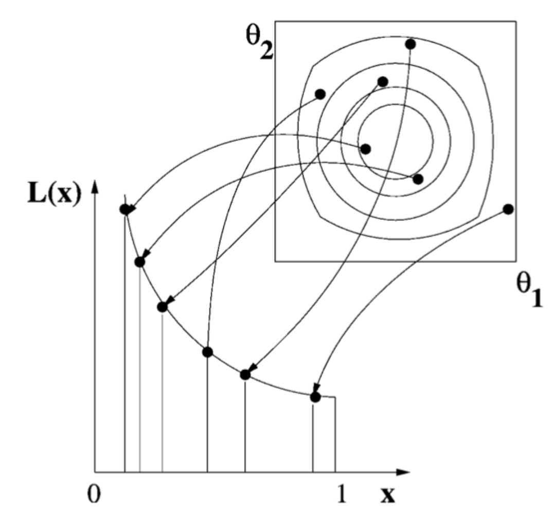
In order to compute the evidence numerically, the prior volume needs to be sampled, in much the same way as in parameter estimation, except the requirements are slightly more stringent. MCMC could be used, although there are claims that it is not good at exploring the parameter space adequately. I find these claims puzzling, as in evidence calculations we are doing an $N$-dimensional integral, which is not so different from doing the $(N-1)$-dimensional integral in MCMC to get marginal errors. However, here are a couple of other sampling techniques.

The VEGAS algorithm, with rotation

This is suitable for single-peaked likelihoods. It is in Numerical Recipes, but needs a modification for efficiency. Essentially, one seeks to sample from a distribution which is close to the target distribution (sampling from a different distribution is called importance sampling), but one does not know what it is yet. One can do this iteratively, sampling from the prior first, then estimating the posterior to get a first guess at the posterior, and using that to refine the sampling distribution.

Now, one does not want to draw randomly from a non-separable function of the parameters, as a moment’s thought will tell you that this is computationally very expensive, so one seeks a separable function, so one can then draw the individual parameters one after the other from $N$ distributions. This works well if the target distribution is indeed separable in the parameters, but not otherwise.

The key extra step [20] is to rotate the parameter axes, which can be done by computing (for example) the moments of the distribution (essentially the moment-of-inertia) after any step, and diagonalising it to find the eigenvectors.

The probability to be sampled is

$$p(\vec{\theta})\propto g_{1}(\theta_{1})g_{2}(\theta_{2})\ldots g_{M}(\theta_{M}).$$ (91)

where it can be shown that

$$g_{\alpha}(\theta_{\alpha})\propto\sqrt{\int_{\beta\neq\alpha}d^{M-1}\theta_{\beta}\frac{f^{2}(\vec{\theta})}{\prod_{\beta\neq\alpha}g_{\beta}(\theta_{\beta})}}$$ (92)

where $f$ is the desired target distribution. Note that $g$ depends on all other $g$s. $g$ can be improved iteratively.

Figure 6: The VEGAS Sampling algorithm, applied to supernova data (from [20]

Nested sampling

Other sampling methods can also be very effective (see e.g. [23, 2, 10, 18]). Nested sampling was introduced by Skilling [21]. One samples from the prior volume, and gradually concentrates more points near the peak of the likelihood distribution, by repeatedly replacing the point with the lowest target density by one drawn strictly from the prior volume with higher target density. This has proved effective for cosmological model selection. I will not go into details here, except to say that the key is in drawing the new point from a suitable subset of the prior volume. This must be increasingly smaller as the points get more confined, otherwise the trial points will be rejected with increasing frequency and it becomes very inefficient, but it must also be a large enough subset that the entire prior volume above the lowest target density is almost certainly included inside. For further details, see the original papers. Note that, for multimodal target distributions, a modification called MultiNest exists [4]. CosmoNest and MultiNest are publicly-available additions to CosmoMC.

Figure 7: The Nested Sampling algorithm. From [18]

6 Summary

We have explored the use of (principally) Bayesian methods for parameter estimation and model selection, and looked at some common numerical methods for performing these tasks. We have also shown how it is possible to work out the (minimum) errors on parameters, and on model probabilities, in advance of doing an experiment, to see if it is worthwhile. These are the common Fisher matrix approach for parameter estimation, and the expected evidence for model selection, which requires no more than the Fisher matrix to compute.

7 Exercises

1. Prove that $({\mathsf{C}}^{-1}),_{\alpha}=-{\mathsf{C}}^{-1}{\mathsf{C}},_{\alpha}{\mathsf{C}}^{-1}$

2. Prove that $(\ln{\mathsf{C}}),_{\alpha}={\mathsf{C}}^{-1}{\mathsf{C}},_{\alpha}$.

3. Prove that $\ln\det{\mathsf{C}}={\rm Tr}\ln{\mathsf{C}}$.

4. A survey is proposed, to determine the mean number density of a certain type of astronomical object, whose positions are random. The survey measures the number of objects in each of $N$ independent cells, such that the mean number per cell, $\bar{n}$, is $\gg 1$. If the cells are observed to have $n_{i}$ objects in them ($i=1,\ldots N$), show that the Fisher matrix (a scalar in this case) for $\bar{n}$ is

$${\mathsf{F}}={N\over 2\bar{n}^{2}}+{N\over\bar{n}}.$$ (93)

Where is most of the information coming from, the dependence of → μ on $\bar{n}$, or $\mathsf{C}$?

Hints:
1. What is ${\mathsf{C}}{\mathsf{C}}^{-1}$?
2. For matrices, $\exp({\mathsf{A}})\equiv{\mathsf{I}}+{\mathsf{A}}+{\mathsf{A}}^{2}/2!+\ldots$. $\ln$ is the inverse of $\exp$.
3. If you rotate coordinate axes (in parameter space in this case), the determinant and trace don’t change.

8 Solutions to exercises

1. Prove that $({\mathsf{C}}^{-1}),_{\alpha}=-{\mathsf{C}}^{-1}{\mathsf{C}},_{\alpha}{\mathsf{C}}^{-1}$

Since ${\mathsf{C}}{\mathsf{C}}^{-1}={\mathsf{I}}$, its derivative is zero. Hence ${\mathsf{C}}({\mathsf{C}}^{-1})_{,\alpha}+{\mathsf{C}}_{,\alpha}{\mathsf{C}}^{-1}=0$. Result follows after premultiplication by ${\mathsf{C}}^{-1}$.

2. Prove that $(\ln{\mathsf{C}}),_{\alpha}={\mathsf{C}}^{-1}{\mathsf{C}},_{\alpha}$.

Let ${\mathsf{A}}=\ln{\mathsf{C}}$, so

$${\mathsf{C}}=\exp{\mathsf{A}}={\mathsf{I}}+{\mathsf{A}}+{{\mathsf{A}}^{2}\over 2!}+\ldots=\sum_{n=0}^{\infty}{{\mathsf{A}}^{n}\over n!}$$

Hence

$${\mathsf{C}}_{,\alpha}=\sum_{n=1}^{\infty}\,{{\mathsf{A}}^{n-1}\over(n-1)!}\,\,{\mathsf{A}}_{,\alpha}=\sum_{m=0}^{\infty}\,{{\mathsf{A}}^{m}\over m!}(\ln{\mathsf{C}})_{,\alpha}={\mathsf{C}}(\ln{\mathsf{C}})_{,\alpha}$$

and result follows.

3. Prove that $\ln\det{\mathsf{C}}={\rm Tr}\ln{\mathsf{C}}$.

${\mathsf{C}}$ is a symmetric matrix and therefore be diagonalised. In the new basis (where we have a new set of parameters which are linear combinations of the old ones), the diagonal components of ${\mathsf{C}}$ are strictly positive (they are variances of the new parameters).

Since the trace and determinant are unchanged by the diagonalisation, we can prove the result in the rotated system. If ${\mathsf{C}}$ is diagonal, then $\ln{\mathsf{C}}$ is diagonal, with components $\ln{\mathsf{C}}_{11},\ \ln{\mathsf{C}}_{22},\ldots$. So ${\rm Tr}\ln{\mathsf{C}}=\sum_{n}{\mathsf{C}}_{nn}$. Since $\det{\mathsf{C}}=\prod_{n}{\mathsf{C}}_{nn}$,

$$\ln\det{\mathsf{C}}=\sum_{n}\ln{\mathsf{C}}_{nn}={\rm Tr}\ln{\mathsf{C}}.$$

This proof is rigorous, but there may be a neater solution without diagonalisation.

4. For $\bar{n}\gg 1$, we can approximate the Poisson distribution by a gaussian, with $\langle n_{i}\rangle=\bar{n}$, and $\sigma_{i}^{2}=\bar{n}$. Hence $\hbox{\vec{\mu}}^{T}=\bar{n}(1,1,\ldots 1)$ and ${\mathsf{C}}=\bar{n}\,{\rm diag}(1,1,\ldots,1)$. Hence ${\mathsf{C}}_{,1}={\rm diag}(1,1,\ldots,1)$, and $M_{ij}$ is an $N\times N$ matrix filled with 2s. The result

$${\mathsf{F}}={N\over 2\bar{n}^{2}}+{N\over\bar{n}}$$ (94)

follows. The first term arises from ${\mathsf{C}}_{,1}$, and the second from $\hbox{\vec{\mu}}_{,1}$. The second dominates since $\bar{n}\gg 1$.

9 Frequently asked questions at the school

Q: My likelihood contours are not elliptical. Am I doing something wrong?
A: No. Likelihood contours are not necessarily elliptical. Close to the peak a Taylor expansion will make them so, but this may well be irrelevant when the likelihood has dropped to where you draw the contours.

Q: How do I include results from more than one experiment?
A: If they are independent, the probabilities multiply, so you just add the $\ln$(likelihood)s. Similarly, you can add Fisher matrices for independent experiments.

References

- (1) Amendola L., Kunz M., Sapone D., JCAP, 04, 013 (2008)
- (2) Beltran M., Garcia-Bellido J., Lesgourgues J., Liddle A. R., Slosar A., 2005, Phys, Rev., D71, 063532
- (3) Duan et al., Phys. Lett. B195, 216 (1987)
- (4) Feroz F., Hobson M., Bridges M., astroph/0809.3437 (2008)
- (5) Fisher R. A., J. Roy. Stat. Soc., 98, 39 (1935)
- (6) Gilks W.R, Richardson S., Spiegelhalter D.J., Markov chain Monte Carlo in practice, Chapman & Hall, London (1996)
- (7) Hajian A., astroph/0608679 (2006)
- (8) Hamilton A.J.S., astroph/0503603 (2005)
- (9) Heavens A.F., Kitching T., Verde L., MNRAS, 380, 1029 (2007).
- (10) Hobson M.P., Bridle S.L., Lahav O., 2002, MNRAS, 335, 377
- (11) Jeffreys H., 1961, Theory of Probability, Oxford University Press (Oxford, UK)
- (12) Kendall M. G., Stuart A., The Advanced Theory of Statistics, Volume II, Griffin, London (1969)
- (13) Kenney, J. F. & Keeping, E. S., Mathematics of Statistics, Part II, 2nd ed. (Van Nostrand, New York) (1951)
- (14) Kosowsky A., Milosavljevic M., Jimenez R., Phys. Rev. D66, 3007 (2002).
- (15) Lazarides, G., Ruiz de Austri, R., Trotta, R., Phys. Rev. D70, 123527
- (16) Lewis A., Bridle S., PRD, 66, 103511 (2002)
- (17) Liddle A., MNRAS, 377, 74 (2007).
- (18) Mukherjee P., Parkinson D., Liddle A.R., 2006, ApJ, 638, L51
- (19) Press W., et al, Numerical Recipes in Fortran, CUP, Cambridge, U.K. (1992)
- (20) Serra P., Heavens A., Melchiorri A., MNRAS 379, 169 (2007)
- (21)
Skilling J., 2004, avaliable at
http://www.inference.phy.cam.ac.uk/bayesys - (22) Tegmark M., Taylor, A.N., Heavens A.F., ApJ, 480, 22 (1997) (TTH)
- (23) Trotta R., 2007, astroph/0703063
- (24) Verde L., astroph/0712.3028 (2007)
- (25) Verde L., et al, ApJS, 148, 195 (2003)