Structured Variable Selection with Sparsity-Inducing Norms

Abstract

We consider the empirical risk minimization problem for linear supervised learning, with regularization by structured sparsity-inducing norms. These are defined as sums of Euclidean norms on certain subsets of variables, extending the usual $\ell_{1}$-norm and the group $\ell_{1}$-norm by allowing the subsets to overlap. This leads to a specific set of allowed nonzero patterns for the solutions of such problems. We first explore the relationship between the groups defining the norm and the resulting nonzero patterns, providing both forward and backward algorithms to go back and forth from groups to patterns. This allows the design of norms adapted to specific prior knowledge expressed in terms of nonzero patterns. We also present an efficient active set algorithm, and analyze the consistency of variable selection for least-squares linear regression in low and high-dimensional settings.

1 Introduction

Regularization by the $\ell_{1}$-norm is now a widespread tool in machine learning, statistics and signal processing: it allows linear variable selection in potentially high dimensions, with both efficient algorithms (Efron et al., 2004; Lee et al., 2007) and well-developed theory for generalization properties and variable selection consistency (Zhao and Yu, 2006; Wainwright, 2009; Bickel et al., 2009; Zhang, 2009).

However, the $\ell_{1}$-norm cannot easily encode prior knowledge about the patterns of nonzero coefficients (“nonzero patterns”) induced in the solution, since they are all theoretically possible. Group $\ell_{1}$-norms (Yuan and Lin, 2006; Roth and Fischer, 2008; Huang and Zhang, 2009) consider a partition of all variables into a certain number of subsets and penalize the sum of the Euclidean norms of each one, leading to selection of groups rather than individual variables. Moreover, recent works have considered overlapping but nested groups in constrained situations such as trees and directed acyclic graphs (Zhao et al., 2008; Bach, 2008c).

In this paper, we consider all possible sets of groups and characterize exactly what type of prior knowledge can be encoded by considering sums of norms of overlapping groups of variables. We first describe how to go from groups to nonzero patterns (or equivalently zero patterns), then show that it is possible to “reverse-engineer” a given set of nonzero patterns, i.e., to build the unique minimal set of groups that will generate these patterns. This allows the automatic design of sparsity-inducing norms, adapted to target sparsity patterns. We give in Section 3 some interesting examples of such designs on two-dimensional grids.

As will be shown in Section 3, for each set of groups, a notion of hull of a nonzero pattern may be naturally defined. In the particular case of the two-dimensional planar grid considered in this paper, this hull is exactly the axis-aligned bounding box or the regular convex hull. We show that, in our framework, the allowed nonzero patterns are exactly those equal to their hull, and that the hull of the relevant variables is consistently estimated under certain conditions, both in low and high-dimensional settings. Moreover, we present in Section 4 an efficient active set algorithm that scales well to high dimensions. Finally, we illustrate in Section 6 the behavior of our norms with synthetic examples on two-dimensional grids.

Notation.

For $x\in\mathbb{R}^{p}$ and $q\in[1,\infty)$, we denote by $\|x\|_{q}$ its $\ell_{q}$-norm defined as $(\sum_{j=1}^{p}|x_{j}|^{q})^{1/q}$ and $\left\|x\right\|_{\infty}=\max_{j\in\{1,\dots,p\}}|x_{j}|$. Given $w\in\mathbb{R}^{p}$ and a subset $J$ of $\{1,\dots,p\}$ with cardinality $|J|$, $w_{J}$ denotes the vector in $\mathbb{R}^{|J|}$ of elements of $w$ indexed by $J$. Similarly, for a matrix $M\in\mathbb{R}^{p\times m}$, $M_{IJ}\in\mathbb{R}^{|I|\times|J|}$ denotes the submatrix of $M$ reduced to the rows indexed by $I$ and the columns indexed by $J$. For any finite set $A$ with cardinality $|A|$, we also define the $|A|$-tuple $(y^{a})_{a\in A}\in\mathbb{R}^{p\times|A|}$ as the collection of $p$-dimensional vectors $y^{a}$ indexed by the elements of $A$. Furthermore, for two vectors $x$ and $y$ in $\mathbb{R}^{p}$, we denote by $x\circ y=(x_{1}y_{1},\dots,x_{p}y_{p})^{\top}\in\mathbb{R}^{p}$ the elementwise product of $x$ and $y$.

2 Regularized Risk Minimization

We consider the problem of predicting a random variable $Y\in\mathcal{Y}$ from a (potentially non random) vector $X\in\mathbb{R}^{p}$, where $\mathcal{Y}$ is the set of responses, typically a subset of $\mathbb{R}$. We assume that we are given $n$ observations $(x_{i},y_{i})\in\mathbb{R}^{p}\times\mathcal{Y}$, $i=1,\dots,n$. We define the empirical risk of a loading vector $w\in\mathbb{R}^{p}$ as $L(w)=\frac{1}{n}\sum_{i=1}^{n}\ell\left(y_{i},w^{\top}x_{i}\right)$, where $\ell:\mathcal{Y}\times\mathbb{R}\mapsto\mathbb{R}^{+}$ is a loss function. We assume that $\ell$ is convex and continuously differentiable with respect to the second parameter. Typical examples of loss functions are the square loss for least squares regression, i.e., $\ell(y,\hat{y})=\frac{1}{2}(y-\hat{y})^{2}$ with $y\in\mathbb{R}$, and the logistic loss $\ell(y,\hat{y})=\log(1+e^{-y\hat{y}})$ for logistic regression, with $y\in\{-1,1\}$.

We focus on a general family of sparsity-inducing norms that allow the penalization of subsets of variables grouped together. Let us denote by $\mathcal{G}$ a subset of the power set of $\{1,\dots,p\}$ such that $\bigcup_{G\in\mathcal{G}}\!G=\{1,\dots,p\}$, i.e., a spanning set of subsets of $\{1,\dots,p\}$. Note that $\mathcal{G}$ does not necessarily define a partition of $\{1,\dots,p\}$, and therefore, it is possible for elements of $\mathcal{G}$ to overlap. We consider the norm $\Omega$ defined by

$$\Omega(w)=\sum_{G\in\mathcal{G}}\left(\sum_{j\in G}(d^{\scriptscriptstyle G}_{j})^{2}|w_{j}|^{2}\right)^{\frac{1}{2}}=\sum_{G\in\mathcal{G}}\left\|d^{\scriptscriptstyle G}\circ w\right\|_{2},$$ (1)

where $(d^{\scriptscriptstyle G})_{G\in\mathcal{G}}$ is a $|\mathcal{G}|$-tuple of $p$-dimensional vectors such that $d^{\scriptscriptstyle G}_{j}>0$ if $j\in G$ and $d^{\scriptscriptstyle G}_{j}=0$ otherwise. Note that a same variable $w_{j}$ belonging to two different groups $G_{1},G_{2}\in\mathcal{G}$ is allowed to be weighted differently in $G_{1}$ and $G_{2}$ (by respectively $d_{j}^{\scriptscriptstyle G_{1}}$ and $d_{j}^{\scriptscriptstyle G_{2}}$). We do not study the more general setting where each $d^{\scriptscriptstyle G}$ would be a (non-diagonal) positive-definite matrix, which we defer for future work.

This general formulation has several important subcases that we present below, the goal of this paper being to go beyond these, and to consider norms capable to incorporate richer prior knowledge.

• $\ell_{2}$-norm: $\mathcal{G}$ is composed of one element, the full set $\{1,\dots,p\}$.

• $\ell_{1}$-norm: $\mathcal{G}$ is the set of all singletons, leading to the Lasso (Tibshirani, 1996) for the square loss.

• $\ell_{2}$-norm and $\ell_{1}$-norm: $\mathcal{G}$ is the set of all singletons and the full set $\{1,\dots,p\}$, leading (up to the squaring of the $\ell_{2}$-norm) to the Elastic net (Zou and Hastie, 2005) for the square loss.

• Group $\ell_{1}$-norm: $\mathcal{G}$ is any partition of $\{1,\dots,p\}$, leading to the group-Lasso for the square loss (Yuan and Lin, 2006).

• Hierarchical norms: when the set $\{1,\dots,p\}$ is embedded into a tree (Zhao et al., 2008) or more generally into a directed acyclic graph (Bach, 2008c), then a set of $p$ groups, each of them composed of descendants of a given variable, is considered.

We study the following regularized problem:

$$\min_{w\in\mathbb{R}^{p}}\ \frac{1}{n}\sum_{i=1}^{n}\ell\left(y_{i},w^{\top}x_{i}\right)+\mu\Omega(w),$$ (2)

where $\mu\!\geq\!0$ is a regularization parameter. Note that a non-regularized constant term could be included in this formulation, but it is left out for simplicity. We denote by $\hat{w}$ any solution of Eq. (2). Regularizing by linear combinations of (non-squared) $\ell_{2}$-norms is known to induce sparsity in $\hat{w}$ (Zhao et al., 2008); our grouping leads to specific patterns that we describe in the next section.

3 Groups and Sparsity Patterns

We now study the relationship between the norm $\Omega$ defined in Eq. (1) and the nonzero patterns the estimated vector $\hat{w}$ is allowed to have. We first characterize the set of nonzero patterns, then we provide forward and backward procedures to go back and forth from groups to patterns.

Figure 1: Groups and induced nonzero pattern: three sparsity-inducing groups (middle and right, denoted by $\{G_{1},G_{2},G_{3}\}$) with the associated nonzero pattern which is the complement of the union of groups, i.e., $(G_{1}\cup G_{2}\cup G_{3})^{c}$ (left, in black).

3.1 Stable Patterns Generated by $\mathcal{G}$

The regularization term $\Omega(w)=\sum_{G\in\mathcal{G}}\left\|d^{\scriptscriptstyle G}\circ w\right\|_{2}$ is a mixed $(\ell_{1},\ell_{2}$)-norm (Zhao et al., 2008). At the group level, it behaves like an $\ell_{1}$-norm and therefore, $\Omega$ induces group sparsity. In other words, each $d^{\scriptscriptstyle G}\circ w$, and equivalently each $w_{G}$ (since the support of $d^{\scriptscriptstyle G}$ is exactly $G$), is encouraged to go to zero. On the other hand, within the groups $G\in\mathcal{G}$, the $\ell_{2}$-norm does not promote sparsity. Intuitively, some of the vectors $w_{G}$ associated with certain groups $G$ will be exactly equal to zero, leading to a set of zeros which is the union of these groups $G$ in $\mathcal{G}$. Thus, the set of allowed zero patterns should be the union-closure of $\mathcal{G}$, i.e. (see Figure 1 for an example):

$$\mathcal{Z}=\left\{\bigcup_{G\in\mathcal{G}^{\prime}}G;\ \mathcal{G}^{\prime}\subseteq\mathcal{G}\right\}.$$ (3)

The situation is however slightly more subtle as some zeros can be created by chance (just as regularizing by the $\ell_{2}$-norm may lead, though it is unlikely, to some zeros). Nevertheless, Theorem 1 (see proof in Appendix A) shows that, under mild conditions, the previous intuition about the set of zero patterns is correct. Note that instead of considering the set of zero patterns $\mathcal{Z}$, it is also convenient to manipulate nonzero patterns, and we define

$$\mathcal{P}=\left\{\bigcap_{G\in\mathcal{G}^{\prime}}G^{c};\ \mathcal{G}^{\prime}\subseteq\mathcal{G}\right\}=\left\{Z^{c};\ Z\in\mathcal{Z}\right\}.$$ (4)

We can equivalently use $\mathcal{P}$ or $\mathcal{Z}$ by taking the complement of each element of these sets. Before stating Theorem 1, we need to introduce the concept of $\mathcal{G}$-adapted hull, or simply hull: for any subset $I\subseteq\{1,\dots,p\}$, we define

$$\mathrm{Hull}(I)=\left\{\bigcup_{G\in\mathcal{G},\ G\cap I=\varnothing}\!\!\!\!G\right\}^{c},$$

which is the smallest set in $\mathcal{P}$ containing $I$ (see Figure 2); we always have $I\subseteq\mathrm{Hull}(I)$ with equality if and only if $I\in\mathcal{P}$. As we shall see later, the hull has a clear geometrical interpretation for specific sets $\mathcal{G}$.

Figure 2: $\mathcal{G}$-adapted hull: the pattern of variables $I$ (left and middle, in red) and its hull (left and right, hatched square) that is defined by the complement of the union of groups that do not intersect $I$, i.e., $(G_{1}\cup G_{2}\cup G_{3})^{c}$.

Theorem 1 (Allowed Patterns).

Assume that $Y=(y_{1},\dots,y_{n})^{\top}$ is a realization of an absolutely continuous probability distribution. Let us consider the following optimization problem

$$\min_{w\in\mathbb{R}^{p}}\ \frac{1}{2n}\sum_{i=1}^{n}(y_{i}-w^{\top}x_{i})^{2}+\mu\Omega(w),$$ (5)

and let denote by $Q$ the Gram matrix $\frac{1}{n}\sum_{i=1}^{n}x_{i}x_{i}^{\top}$.

If for all solution $\hat{w}$ of (5) with nonzero pattern $\hat{I}=\{j\in\{1,\dots,p\};\ \hat{w}_{j}\neq 0\}$, the matrix $Q_{\mathrm{Hull}(\hat{I})\mathrm{Hull}(\hat{I})}$ is invertible, then the problem (5) has a unique solution whose set of zeros is in $\mathcal{Z}=\left\{\bigcup_{G\in\mathcal{G}^{\prime}}G;\ \mathcal{G}^{\prime}\subseteq\mathcal{G}\right\}$ almost surely.

In particular, the above result implies that almost surely Eq. (5) has a unique solution when the full matrix $Q$ is invertible. Nevertheless, Theorem 1 does not require the invertibility of the full matrix $Q$. The result can therefore hold in high-dimensional settings where the number of observations $n$ is smaller than the number of variables $p$ (in this case, Q is always singular).

We have the following usual special cases from Section 2 (we give more examples in Section 3.5):

• $\ell_{2}$-norm: the set of allowed nonzero patterns is composed of the empty set and the full set $\{1,\dots,p\}$.

• $\ell_{1}$-norm: $\mathcal{P}$ is the set of all possible subsets.

• $\ell_{2}$-norm and $\ell_{1}$-norm: $\mathcal{P}$ is also the set of all possible subsets.

• Grouped $\ell_{1}$-norm: $\mathcal{P}=\mathcal{Z}$ is the set of all possible unions of the elements of the partition defining $\mathcal{G}$.

• Hierarchical norms: the set of patterns $\mathcal{P}$ is then all sets $J$ for which all ancestors of elements in $J$ are included in $J$ (Bach, 2008c).

Two natural questions arise: (1) starting from the groups $\mathcal{G}$, is there an efficient way to generate the set of nonzero patterns $\mathcal{P}$; (2) conversely, and more importantly, given $\mathcal{P}$, how can the groups $\mathcal{G}$—and hence the norm $\Omega(w)$—be designed?

3.2 General Properties of $\mathcal{G}$, $\mathcal{Z}$ and $\mathcal{P}$

Closedness.

The set of zero patterns $\mathcal{Z}$ (respectively, the set of nonzero patterns $\mathcal{P}$) is closed under union (respectively, intersection), that is, for all $K\in\mathbb{N}$ and all $z_{1},\dots,z_{K}\in\mathcal{Z},\ \bigcup_{k=1}^{K}z_{k}\in\mathcal{Z}$ (respectively, $p_{1},\dots,p_{K}\in\mathcal{P},\ \bigcap_{k=1}^{K}p_{k}\in\mathcal{P}$). This implies that when “reverse-engineering” the set of nonzero patterns, we have to assume it is closed under intersection. Otherwise, the best we can do is to deal with its intersection-closure.

Minimality.

If a group in $\mathcal{G}$ is the union of other groups, it may be removed from $\mathcal{G}$ without changing the sets $\mathcal{Z}$ or $\mathcal{P}$. This is the main argument behind the pruning backward algorithm in Section 3.4. Moreover, this leads to the notion of a minimal set $\mathcal{G}$ of groups, which is such that for all $\mathcal{G}^{\prime}\subseteq\mathcal{Z}$ whose union-closure spans $\mathcal{Z}$, we have $\mathcal{G}\subseteq\mathcal{G}^{\prime}$. The existence and unicity of a minimal set is a consequence of classical results in set theory (Doignon and Falmagne, 1998). The elements of this minimal set are usually referred to as the atoms of $\mathcal{Z}$.

Minimal sets of groups are attractive in our setting because they lead to a smaller number of groups and lower computational complexity—for example, for 2 dimensional-grids with rectangular patterns, we have a quadratic possible number of rectangles, i.e., $|\mathcal{Z}|=O(p^{2})$, that can be generated by a minimal set $\mathcal{G}$ whose size is $|\mathcal{G}|=O(\sqrt{p})$.

Hull.

We recall the definition of the $\mathcal{G}$-adapted hull, namely, for any subset $I\subseteq\{1,\dots,p\}$,

$$\mathrm{Hull}(I)=\left\{\bigcup_{G\in\mathcal{G},G\cap I=\varnothing}\!\!\!\!G\right\}^{c},$$

which is the smallest set in $\mathcal{P}$ containing $I$.

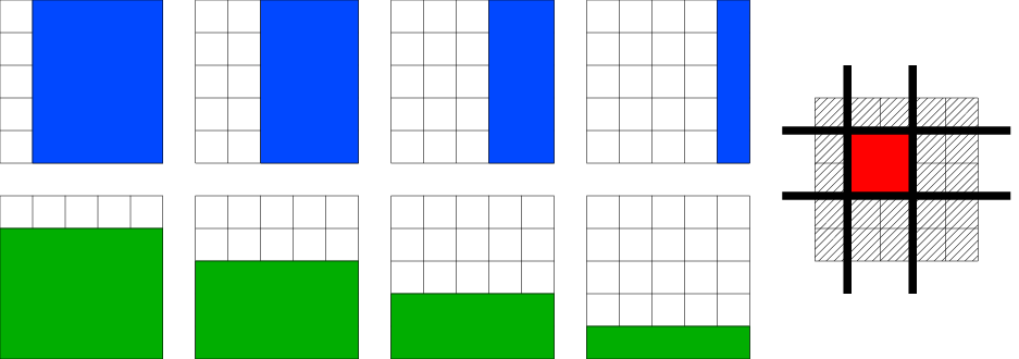
If the set $\mathcal{G}$ is formed by all vertical and horizontal half-spaces when the variables are organized in a 2 dimensional-grid (see Figure 5), the hull of a subset $I\subset\{1,\dots,p\}$ is simply the axis-aligned bounding box of $I$. Similarly, when $\mathcal{G}$ is the set of all half-spaces with all orientations (e.g., orientations $\pm\pi/4$ are shown in Figure 6), the hull becomes the regular convex hull. Note that those interpretations of the hull are possible and valid only when we have geometrical information at hand about the set of variables.

Graphs of patterns.

We consider the directed acyclic graph (DAG) stemming from the Hasse diagram of the partially ordered set (poset) $(\mathcal{G},\supset)$. The nodes of this graph are the elements $G$ of $\mathcal{G}$ and there is a directed edge from $G_{1}$ to $G_{2}$ if and only if $G_{1}\supset G_{2}$ and there exists no $G\in\mathcal{G}$ such that $G_{1}\supset G\supset G_{2}$ (Cameron, 1994). We can also build the corresponding DAG for the set of zero patterns $\mathcal{Z}\supset\mathcal{G}$, which is a super-DAG of the DAG of groups (see Figure 3 for examples). Note that we obtain also the isomorphic DAG for the nonzero patterns $\mathcal{P}$, although it corresponds to the poset $(\mathcal{P},\subset)$: this DAG will be used in the active set algorithm presented in Section 4.

Prior works with nested groups (Zhao et al., 2008; Bach, 2008c) have used a similar DAG, which was isomorphic to a DAG on the variables because of the specificity of the hierarchical norm. As opposed to those cases where the DAG was used to give an additional structure to the problem, the DAG we introduce here on the set of groups naturally and always comes up, with no assumption on the variables themselves (for which no DAG is defined in general).

Figure 3: The DAG for the set $\mathcal{Z}$ associated with the $2\!\times\!2$-grid. The members of $\mathcal{Z}$ are the complement of the areas hatched in black. The elements of $\mathcal{G}$ (i.e., the atoms of $\mathcal{Z}$) are highlighted by bold edges.

3.3 From Groups to Patterns

The forward procedure presented in Algorithm 1, taken from Doignon and Falmagne (1998), allows the construction of $\mathcal{Z}$ from $\mathcal{G}$. It iteratively builds the collection of patterns by taking unions, and has complexity $O(p|\mathcal{Z}||\mathcal{G}|^{2})$. The general scheme is straightforward. Namely, by considering increasingly larger subfamilies of $\mathcal{G}$ and the collection of patterns already obtained, all possible unions are formed. However, some attention needs to be paid while checking we are not generating a pattern already encountered. Such a verification is performed by the if condition within the inner loop of the algorithm. Indeed, we do not have to scan the whole collection of patterns already obtained (whose size can be exponential in $|\mathcal{G}|$), but we rather use the fact that $\mathcal{G}$ generates $\mathcal{Z}$. Note that in general, it is not possible to upper bound the size of $|\mathcal{Z}|$ by a polynomial term in $p$, even when $\mathcal{G}$ is very small (indeed, $|\mathcal{Z}|=2^{p}$ for the $\ell_{1}$-norm).

Algorithm 1 Forward procedure

 Input: Set of groups $\mathcal{G}=\{G_{1},\dots,G_{M}\}$.

 Output: Collection of zero patterns $\mathcal{Z}$ and nonzero patterns $\mathcal{P}$.

 Intialization: $\mathcal{Z}=\{\varnothing\}$.

 for $m=1$ to $M$ do

  $C=\{\varnothing\}$

  for each $Z\in\mathcal{Z}$ do

   if $\left(G_{m}\nsubseteq Z\right)$ and $(\forall G\in\!\{G_{1},\dots,G_{m-1}\},\ G\subseteq Z\cup G_{m}\Rightarrow G\subseteq Z)$ then

    $C\leftarrow C\cup\{Z\cup G_{m}\}$ .

   end if

  end for$\mathcal{Z}\leftarrow\mathcal{Z}\cup C$.

 end for$\mathcal{P}=\left\{Z^{c};\ Z\in\mathcal{Z}\right\}$.

3.4 From Patterns to Groups

We now assume that we want to impose a priori knowledge on the sparsity structure of $\hat{w}$. This information can be exploited by restricting the patterns allowed by the norm $\Omega$. Namely, from an intersection-closed set of zero patterns $\mathcal{Z}$, we can build back a minimal set of groups $\mathcal{G}$ by iteratively pruning away in the DAG corresponding to $\mathcal{Z}$, all sets which are unions of their parents. See Algorithm 2.

Algorithm 2 Backward procedure

 Input: Intersection-closed family of nonzero patterns $\mathcal{P}$.

 Output: Set of groups $\mathcal{G}$.

 Initialization: Compute $\mathcal{Z}=\left\{P^{c};\ P\in\mathcal{P}\right\}$ and set $\mathcal{G}=\mathcal{Z}$.Build the Hasse diagram for the poset $(\mathcal{Z},\supset)$.

 for $t=\min_{G\in\mathcal{Z}}|G|$ to $\max_{G\in\mathcal{Z}}|G|$ do

  for each node $G\in\mathcal{Z}$ such that $|G|=t$ do

   if $\left(\bigcup_{C\in\textrm{Children}(G)}C=G\right)$ then

    if $\left(\textrm{Parents}(G)\neq\varnothing\right)$ then

     Connect children of $G$ to parents of $G$.

    end if

    Remove $G$ from $\mathcal{G}$.

   end if

  end for

 end for

This algorithm can be found under a different form in  (Doignon and Falmagne, 1998)—we present it through a pruning algorithm on the DAG, which is natural in our context (the proof of the minimality of the procedure can be found in Appendix B). The complexity of Algorithm 2 is $O(p|\mathcal{Z}|^{2})$. The pruning may reduce significantly the number of groups necessary to generate the whole set of zero patterns, sometimes from exponential in $p$ to polynomial in $p$ (e.g., the $\ell_{1}$-norm). We now give examples where $|\mathcal{G}|$ is also polynomial in $p$.

3.5 Examples

Sequences.

Given $p$ variables organized in a sequence, if we want only contiguous nonzero patterns, the backward algorithm will lead to the set of groups which are intervals $[1,k]_{k\in\{1,\dots,p-1\}}$ and $[k,p]_{k\in\{2,\dots,p\}}$, with both $|\mathcal{Z}|=O(p^{2})$ and $|\mathcal{G}|=O(p)$ (see Figure 4).

Figure 4: (Left) The set of blue groups to penalize in order to select contiguous patterns in a sequence. (Right) In red, an example of such a pattern.

Two-dimensional grids.

In Section 6, we notably consider for $\mathcal{P}$ the set of all rectangles in two dimensions, leading by the previous algorithm to the set of axis-aligned half-spaces for $\mathcal{G}$ (see Figure 5), with $|\mathcal{Z}|=O(p^{2})$ and $|\mathcal{G}|=O(\sqrt{p})$. This type of structure is encountered in object or scene recognition, where the selected rectangle would correspond to a certain box inside an image, that concentrates the predictive power for a given class of object/scene.

By adding half-planes to $|\mathcal{G}|$ with different orientations than $0$ and $\pi/2$, the set of nonzero patterns $\mathcal{P}$ tends to the convex set in the two-dimensional grid (Soille, 2003). See Figure 6. The number of groups is linear in $\sqrt{p}$ with constant growing linearly with the number of angles, while $|\mathcal{Z}|$ grows more rapidly (typically non-polynomially in the number of angles). This type of structure could be useful in vision as well as in neuroscience, in particular to retrieve brain activity in EEG data, which is usually a small convex-like portion of the scalp.

Figure 5: Vertical and horizontal groups: (Left) the set of blue and green groups with their (not displayed) complements to penalize in order to select rectangles. (Right) In red, an example of recovered pattern in this setting.

Figure 6: Groups with $\pm\pi/4$ orientations: (Left) the set of blue and green groups with their (not displayed) complements to penalize in order to select diamond-shaped patterns. (Right) In red, an example of recovered pattern in this setting.

Extensions.

The sets of groups presented above can be straightforwardly extended to more complicated topologies, such as three-dimensional spaces discretized in cubes or spherical volumes discretized in slices. Similar proporties hold for such settings. For instance, if all the axis-aligned half-spaces are considered for $\mathcal{G}$ in a three-dimensional space, then $\mathcal{P}$ is the set of all possible rectangular boxes with $|\mathcal{P}|=O(p^{2})$ and $|\mathcal{G}|=O(p^{1/3})$ (see Jenatton et al. (2009) for a biological application with such groups).

4 Optimization and Active Set Algorithm

For moderate values of $p$, one may obtain a solution for Eq. (2) using generic toolboxes for second-order cone programming (SOCP) whose time complexity is equal to $O(p^{3.5}+|\mathcal{G}|^{3.5})$ (Boyd and Vandenberghe, 2004), which is not appropriate when $p$ or $|\mathcal{G}|$ are large.

We present in this section an active set algorithm (Algorithm 3) that finds a solution for Eq. (2) by considering increasingly larger active sets and checking global optimality at each step, with total complexity in $O(p^{1.75})$. Here, the sparsity prior is exploited for computational advantages. Our active set algorithm needs an underlying black-box solver; in this paper, we consider both a first order approach (see Appendix G) and a SOCP method — in our experiments, we use SDPT3 (Toh et al., 1999; Tütüncü et al., 2003). Our active set algorithm extends to general overlapping groups the work of Bach (2008c), by further assuming that it is computationally possible to be polynomial in the number of variables $p$.

4.1 Optimality Conditions: from Reduced Problems to Full Problems

It is simpler to derive the algorithm for the following regularized optimization problem which has the same solution set as the regularized problem of Eq. (2) when $\mu$ and $\lambda$ are allowed to vary (Borwein and Lewis, 2006, see Section 3.2):

$$\min_{w\in\mathbb{R}^{p}}\frac{1}{n}\sum_{i=1}^{n}\ell\left(y_{i},w^{\top}x_{i}\right)+\frac{\lambda}{2}\left[\Omega(w)\right]^{2}.$$ (6)

In active set methods, the set of nonzero variables, denoted by $J$, is built incrementally, and the problem is solved only for this reduced set of variables, adding the constraint $w_{J^{c}}=0$ to Eq. (6). We denote by $L(w)=\frac{1}{n}\sum_{i=1}^{n}\ell\left(y_{i},w^{\top}x_{i}\right)$ the empirical risk (which is by assumption convex and continuously differentiable) and by $L^{\ast}$ its Fenchel-conjugate, defined as (Borwein and Lewis, 2006):

$$L^{\ast}(u)=\sup_{w\in\mathbb{R}^{p}}\{w^{\top}u-L(w)\}.$$

The restriction of $L$ to $\mathbb{R}^{|J|}$ is denoted $L_{J}(w_{J})=L(\tilde{w})$ for $\tilde{w}_{J}=w_{J}$ and $\tilde{w}_{J^{c}}=0$, with Fenchel-conjugate $L_{J}^{\ast}$. Note that, as opposed to $L$, we do not have $L_{J}^{\ast}(\kappa_{J})=L^{\ast}(\tilde{\kappa})$ for $\tilde{\kappa}_{J}=\kappa_{J}$ and $\tilde{\kappa}_{J^{c}}=0$.

For a potential active set $J\subset\{1,\dots,p\}$ which belongs to the set of allowed nonzero patterns $\mathcal{P}$, we denote by $\mathcal{G}_{J}$ the set of active groups, i.e., the set of groups $G\in\mathcal{G}$ such that $G\cap J\neq\varnothing$. We consider the reduced norm $\Omega_{J}$ defined on $\mathbb{R}^{|J|}$ as

$$\Omega_{J}(w_{J})=\sum_{G\in\mathcal{G}}\left\|d^{\scriptscriptstyle G}_{J}\circ w_{J}\right\|_{2}=\sum_{G\in\mathcal{G}_{J}}\left\|d^{\scriptscriptstyle G}_{J}\circ w_{J}\right\|_{2},$$

and its dual norm $\Omega_{J}^{*}(\kappa_{J})=\max_{\Omega_{J}(w_{J})\leq 1}w_{J}^{\top}\kappa_{J}$. The next proposition (see proof in Appendix C) gives the optimization problem dual to the reduced problem (Eq. (7) below):

Proposition 2 (Dual Problems).

Let $J\subseteq\{1,\dots,p\}$. The following two problems

$$\min_{w_{J}\in\mathbb{R}^{|J|}}L_{J}(w_{J})+\frac{\lambda}{2}\left[\Omega_{J}(w_{J})\right]^{2},$$ (7)

$$\max_{\kappa_{J}\in\mathbb{R}^{|J|}}\ -L_{J}^{*}(-\kappa_{J})-\frac{1}{2\lambda}\left[\Omega_{J}^{*}(\kappa_{J})\right]^{2},$$ (8)

are dual to each other and the pair of primal-dual variables $\{w_{J},\kappa_{J}\}$ is optimal if and only if we have

$$\begin{cases}\kappa_{J}&=-\nabla L_{J}(w_{J}),\\ w_{J}^{\top}\kappa_{J}&=\frac{1}{\lambda}\left[\Omega_{J}^{*}(\kappa_{J})\right]^{2}=\lambda\left[\Omega_{J}(w_{J})\right]^{2}.\end{cases}$$

The duality gap of the previous optimization problem is

$$L_{J}(w_{J})+L_{J}^{*}(-\kappa_{J})+\frac{\lambda}{2}\left[\Omega_{J}(w_{J})\right]^{2}+\frac{1}{2\lambda}\left[\Omega_{J}^{*}(\kappa_{J})\right]^{2}$$

$$= \left\{L_{J}(w_{J})+L_{J}^{*}(-\kappa_{J})+w_{J}^{\top}\kappa_{J}\right\}+\left\{\frac{\lambda}{2}\left[\Omega_{J}(w_{J})\right]^{2}+\frac{1}{2\lambda}\left[\Omega_{J}^{*}(\kappa_{J})\right]^{2}-w_{J}^{\top}\kappa_{J}\right\},$$

which is a sum of two nonnegative terms, the nonnegativity coming from the Fenchel-Young inequality (Borwein and Lewis, 2006, Proposition 3.3.4). We can think of this duality gap as the sum of two duality gaps, relative to $L_{J}$ and $\Omega_{J}$. Thus, if we have a primal candidate $w_{J}$ and we choose $\kappa_{J}=-\nabla L_{J}(w_{J})$, the duality gap relative to $L_{J}$ vanishes and the total duality gap then reduces to

$$\frac{\lambda}{2}\left[\Omega_{J}(w_{J})\right]^{2}+\frac{1}{2\lambda}\left[\Omega_{J}^{*}(\kappa_{J})\right]^{2}-w_{J}^{\top}\kappa_{J}.$$

In order to check that the reduced solution $w_{J}$ is optimal for the full problem in Eq. (6), we pad $w_{J}$ with zeros on ${J^{c}}$ to define $w$, compute $\kappa=-\nabla L(w)$, which is such that $\kappa_{J}=-\nabla L_{J}(w_{J})$, and get a duality gap for the full problem equal to

$$\frac{\lambda}{2}\left[\Omega(w)\right]^{2}+\frac{1}{2\lambda}\left[\Omega^{*}(\kappa)\right]^{2}-w^{\top}\kappa$$

$$= \frac{\lambda}{2}\left[\Omega(w)\right]^{2}+\frac{1}{2\lambda}\left[\Omega^{*}(\kappa)\right]^{2}-w_{J}^{\top}\kappa_{J}$$

$$= \frac{\lambda}{2}\left[\Omega(w)\right]^{2}+\frac{1}{2\lambda}\left[\Omega^{*}(\kappa)\right]^{2}-\frac{\lambda}{2}\left[\Omega_{J}(w_{J})\right]^{2}-\frac{1}{2\lambda}\left[\Omega_{J}^{*}(\kappa_{J})\right]^{2}$$

$$= \frac{1}{2\lambda}\left(\left[\Omega^{*}(\kappa)\right]^{2}-\left[\Omega_{J}^{*}(\kappa_{J})\right]^{2}\right)$$

$$= \frac{1}{2\lambda}\left(\left[\Omega^{*}(\kappa)\right]^{2}-\lambda w_{J}^{\top}\kappa_{J}\right).$$

Computing this gap requires solving an optimization problem which is as hard as the original one, prompting the need for upper and lower bounds on $\Omega^{*}$ (see Propositions 3 and 4 for more details).

4.2 Active set algorithm

In light of Theorem 1, we can interpret the active set algorithm as a walk through the DAG of nonzero patterns allowed by the norm $\Omega$. The parents $\Pi_{\mathcal{P}}(J)$ of $J$ in this DAG are exactly the patterns containing the variables that may enter the active set at the next iteration of Algorithm 3. The groups that are exactly at the boundaries of the active set (referred to as the fringe groups) are $\mathcal{F}_{J}=\{G\in(\mathcal{G}_{J})^{c}\ ;\ \nexists G^{\prime}\in(\mathcal{G}_{J})^{c},\ G\subseteq G^{\prime}\}$, i.e., the groups that are not contained by any other inactive groups.

In simple settings, e.g., when $\mathcal{G}$ is the set of rectangular groups, the correspondance between groups and variables is straightforward since we have $\mathcal{F}_{J}=\bigcup_{K\in\Pi_{\mathcal{P}}(J)}\mathcal{G}_{K}\backslash\mathcal{G}_{J}$ (see Figure 7). Hovewer, in general, we just have the inclusion $(\bigcup_{K\in\Pi_{\mathcal{P}}(J)}\mathcal{G}_{K}\backslash\mathcal{G}_{J})\subseteq\mathcal{F}_{J}$ and some elements of $\mathcal{F}_{J}$ might not correspond to any patterns of variables in $\Pi_{\mathcal{P}}(J)$ (see Figure 8).

Figure 7: The active set (black) and the candidate patterns of variables, i.e. the variables in $K\backslash J$ (hatched in black) that can become active. The fringe groups are exactly the groups that have the hatched areas (i.e., here we have $\mathcal{F}_{J}=\bigcup_{K\in\Pi_{\mathcal{P}}(J)}\mathcal{G}_{K}\backslash\mathcal{G}_{J}=\{G_{1},G_{2},G_{3}\}$).

Figure 8: The active set (black) and the candidate patterns of variables, i.e. the variables in $K\backslash J$ (hatched in black) that can become active. The groups in red are those in $\bigcup_{K\in\Pi_{\mathcal{P}}(J)}\mathcal{G}_{K}\backslash\mathcal{G}_{J}$, while the blue group is in $\mathcal{F}_{J}\backslash(\bigcup_{K\in\Pi_{\mathcal{P}}(J)}\mathcal{G}_{K}\backslash\mathcal{G}_{J})$. The blue group does not intersect with any patterns in $\Pi_{\mathcal{P}}(J)$.

We now present the optimality conditions (see proofs in Appendix D) that monitor the progress of Algorithm 3 :

Proposition 3 (Necessary condition).

If $w$ is optimal for the full problem in Eq. (6), then

$$\max_{K\in\Pi_{\mathcal{P}}(J)}\dfrac{\left\|\nabla L(w)_{K\backslash J}\right\|_{2}}{\sum_{H\in\mathcal{G}_{K}\backslash\mathcal{G}_{J}}\left\|d^{\scriptscriptstyle H}_{\scriptscriptstyle K\backslash J}\right\|_{\infty}}\leqslant\big\{\!\!-\lambda w^{\top}\nabla L(w)\big\}^{\frac{1}{2}}. N$$ ()

Proposition 4 (Sufficient condition).

If

$$\max_{G\in\mathcal{F}_{J}}\left\{\sum_{k\in G}\bigg\{\dfrac{\nabla L(w)_{k}}{\sum_{H\ni k,\ H\in(\mathcal{G}_{J})^{c}}d^{\scriptscriptstyle H}_{k}}\bigg\}^{2}\right\}^{\frac{1}{2}}\!\leqslant\big\{\lambda(2\varepsilon-w^{\top}\nabla L(w))\big\}^{\frac{1}{2}}, S_{\varepsilon}$$ ()

then $w$ is a solution for Eq. (6) whose duality gap is less than $\varepsilon\geq 0$.

Note that for the Lasso, the conditions $(N)$ and $(S_{0})$ (i.e., the sufficient condition taken with $\varepsilon=0$) are both equivalent (up to the squaring of $\Omega$) to the condition $\|\nabla L(w)_{J^{c}}\|_{\infty}\leqslant-w^{\top}\nabla L(w)$, which is the usual optimality condition (Wainwright, 2009; Tibshirani, 1996). Moreover, when they are not satisfied, our two conditions provide good heuristics for choosing which $K\in\Pi_{\mathcal{P}}(J)$ should enter the active set.

More precisely, since the necessary condition ( N ) directly deals with the variables (as opposed to groups) that can become active at the next step of Algorithm 3, it suffices to choose the pattern $K\in\Pi_{\mathcal{P}}(J)$ that violates the condition most.

The heuristics for the sufficient condition ( S ε ) implies to go from groups to variables. We simply consider the group $G\in\mathcal{F}_{J}$ that violates the sufficient condition most and then take all the patterns of variables $K\in\Pi_{\mathcal{P}}(J)$ such that $\ K\cap G\neq\varnothing$ to enter the active set. If $G\cap(\bigcup_{K\in\Pi_{\mathcal{P}}(J)}K)=\varnothing$, we look at all the groups $H\in\mathcal{F}_{J}$ such that $H\cap G\neq\varnothing$ and apply the scheme described before (see Algorithm 4).

A direct consequence of this heuristics is that it is possible for the algorithm to jump over the right active set and to consider instead a (slightly) larger active set as optimal. However if the active set is larger than the optimal set, then (it can be proved that) the sufficient condition $(S_{0})$ is satisfied, and the reduced problem, which we solve exactly, will still output the correct nonzero pattern.

Moreover, it is worthwile to notice that in Algorithm 3, the active set may sometimes be increased only to make sure that the current solution is optimal (we only check a sufficient condition of optimality).

Algorithm 3 Active set algorithm

 Input: Data $\{(x_{i},y_{i})$, $i=1,\dots,n\}$, regularization parameter $\lambda$,     Duality gap precision $\varepsilon$, maximum number of variables $s$.

 Output: Active set $J$, loading vector $\hat{w}$.

 Intialization: $J=\{\varnothing\}$, $\hat{w}=0$.

 while $\big($ $(N)$ is not satisfied $\big)$ and $\big($ $|J|\leqslant s$ $\big)$ do

  Replace $J$ by violating $K\in\Pi_{\mathcal{P}}(J)$ in ( N ).

  Solve the reduced problem $\,\min_{w_{J}\in\mathbb{R}^{|J|}}L_{J}(w_{J})+\frac{\lambda}{2}\left[\Omega_{J}(w_{J})\right]^{2}\,$ to get $\hat{w}$.

 end while

 while $\big($ $(S_{\varepsilon})$ is not satisfied $\big)$ and $\big($ $|J|\leqslant s$ $\big)$ do

  Update $J$ according to Algorithm 4.

  Solve the reduced problem $\,\min_{w_{J}\in\mathbb{R}^{|J|}}L_{J}(w_{J})+\frac{\lambda}{2}\left[\Omega_{J}(w_{J})\right]^{2}\,$ to get $\hat{w}$.

 end while

Convergence of the active set algorithm.

The procedure described in Algorithm 3 can terminate in two different states. If the procedure stops because of the limit on the number of active variables $s$, the solution might be suboptimal with a nonzero pattern smaller than the optimal one.

Otherwise, the procedure always converges to an optimal solution, either (1) by validating both the necessary and sufficient conditions (see Propositions 3 and 4), ending up with fewer than $p$ active variables and a precision of (at least) $\varepsilon$, or (2) by running until the $p$ variables become active, the precision of the solution being given by the underlying solver.

Algorithmic complexity.

We analyse in detail the time complexity of the active set algorithm when we consider sets of groups $\mathcal{G}$ such as those presented in the examples of Section 3.5, i.e., collections of nested groups with $n_{\theta}$ different orientations. For instance, when we deal with sequences (see Figure 4), we have $n_{\theta}=2$ orientations. Note that for such choices of $\mathcal{G}$, the fringe groups $\mathcal{F}_{J}$ reduces to the largest groups of each orientation and therefore $|\mathcal{F}_{J}|\leq n_{\theta}$. We further assume that $\mathcal{G}$ is sorted by cardinality and by orientation, so that computing $\mathcal{F}_{J}$ costs $O(1)$.

Given an active set $J$, both the necessary and sufficient conditions require to have access to the direct parents $\Pi_{\mathcal{P}}(J)$ of $J$ in the DAG of nonzero patterns. In simple settings, e.g., when $\mathcal{G}$ is the set of rectangular groups, this operation can be performed in $O(1)$ (it just corresponds to scan the (up to) four patterns at the edges of the current rectangular hull).

Hovewer, for more general orientations, computing $\Pi_{\mathcal{P}}(J)$ requires to find the smallest nonzero patterns that we can generate from the groups in $\mathcal{F}_{J}$, reduced to the stripe of variables around the current hull. This stripe of variables can be computed as $\scriptstyle\left[\bigcup_{G\in(\mathcal{G}_{J})^{c}\backslash\mathcal{F}_{J}}G\right]^{c}\backslash J$, so that getting $\Pi_{\mathcal{P}}(J)$ costs $O(s2^{n_{\theta}}+p|\mathcal{G}|)$ in total.

Thus, if the number of active variables is upper bounded by $s\!\ll\!p$ (which is true if our target is actually sparse), the time complexity of Algorithm 3 is the sum of:

• the computation of the gradient, $O(snp)$ for the square loss.

• if the underlying solver called upon by the active set algorithm is a standard SOCP solver, $O(s\max_{J\in\mathcal{P},|J|\leqslant s}|\mathcal{G}_{J}|^{3.5}+s^{4.5})$ (note that the term $s^{4.5}$ could be improved upon by using warm-restart strategies for the sequence of reduced problems).

• $t_{1}$ times the computation of $(N)$, that is $O(t_{1}(s2^{n_{\theta}}+p|\mathcal{G}|+sn_{\theta}^{2})+p|\mathcal{G}|)=O(t_{1}p|\mathcal{G}|)$.

  During the initialization (i.e., $J=\varnothing$), we have $|\Pi_{\mathcal{P}}(\varnothing)|=O(p)$ (since we can start with any singletons), and $|\mathcal{G}_{K}\backslash\mathcal{G}_{J}|=|\mathcal{G}_{K}|=|\mathcal{G}|$, which leads to a complexity of $O(p|\mathcal{G}|)$ for the sum $\sum_{G\in\mathcal{G}_{K}\backslash\mathcal{G}_{J}}=\sum_{G\in\mathcal{G}_{K}}$. Note however that this sum does not depend on $J$ and can therefore be cached if we need to make several runs with the same set of groups $\mathcal{G}$.

• $t_{2}$ times the computation of $(S_{\varepsilon})$, that is $O(t_{2}(s2^{n_{\theta}}+p|\mathcal{G}|+n_{\theta}^{2}+n_{\theta}p+p|\mathcal{G}|))=O(t_{2}p|\mathcal{G}|)$, with $t_{1}+t_{2}\leq s$.

We finally get complexity with a leading term in $O(sp|\mathcal{G}|+s\max_{J\in\mathcal{P},|J|\leqslant s}|\mathcal{G}_{J}|^{3.5})$, which is much better than $O(p^{3.5}+|\mathcal{G}|^{3.5})$, without an active set method. In the example of the two-dimensional grid (see Section 3.5), we have $|\mathcal{G}|=O(\sqrt{p})$ and a total complexity in $O(sp^{1.75})$. Note that we have derived here the theoritical complexity of the active set algorithm when we use a SOCP method as underlying solver. With the first order method presented in Appendix G, we would instead get a total complexity in $O(sp^{1.5})$.

Algorithm 4 Heuristics for the sufficient condition ( S ε )

 Let $G\in\mathcal{F}_{J}$ be the group that violates ( S ε ) most.

 if $(G\cap(\bigcup_{K\in\Pi_{\mathcal{P}}(J)}K)\neq\varnothing)$ then

  for $K\in\Pi_{\mathcal{P}}(J)$ such that $K\cap G\neq\varnothing$ do

   $J\leftarrow J\cup K$.

  end for

 else

  for $H\in\mathcal{F}_{J}$ such that $H\cap G\neq\varnothing$ do

   for $K\in\Pi_{\mathcal{P}}(J)$ such that $K\cap H\neq\varnothing$ do

    $J\leftarrow J\cup K$.

   end for

  end for

 end if

4.3 Intersecting Nonzero Patterns.

We have seen so far how overlapping groups can encore prior information about a desired set of (non)zero patterns. In practice, controlling these overlaps may be delicate and hinges on the choice of the weights $(d^{\scriptscriptstyle G})_{G\in\mathcal{G}}$ (see the experiments in Section 6). In particular, the weights have to take into account that some variables belonging to several overlapping groups are more penalized.

Hovewer, it is possible to keep the benefit of overlapping groups whilst limiting their side effects, by taking up the idea of support intersection (Bach, 2008a; Meinshausen and Bühlmann, 2008). First introduced to stabilize the set of variables recovered by the Lasso, we reuse this technique in a different context, based on the following remark.

Since $\mathcal{P}$ is closed under intersection, when we deal with collections of nested groups with multiple orientations, the two procedures described below actually lead to the same set of allowed (non)zero patterns:

• Considering one model with the norm $\Omega$ composed of all the groups (i.e., the groups for all the orientations).

• First considering one model per orientation (the norm $\Omega$ of this model being only comprised of the nested groups corresponding to that orientation) and then taking the intersection of the nonzero patterns obtained for each of those models. In the example of the sequence (see Figure 4), it boils down to considering one model with the groups starting from the left and one model with the groups starting from the right.

Note that, with this method, although the training of several models is required (a number of times equals to the number of orientations considered, e.g., 2 for the sequence and 4 for the rectangular groups), each of those trainings involves a smaller number of groups. In addition, this procedure is a variable selection technique that therefore needs a second step for estimating the loadings (restricted to the selected nonzero pattern). In the experiments, we follow Bach (2008a) and we use an ordinary least squares (OLS). The simulations of Section 6 will show the superiority of this variable selection approach.

5 Pattern Consistency

In this section, we analyze the model consistency of the solution of Eq. (2) for the square loss. Considering the set of nonzero patterns $\mathcal{P}$ derived in Section 3, we can only hope to estimate the correct hull of the generating sparsity pattern, since Theorem 1 states that other patterns occur with zero probability. We derive necessary and sufficient conditions for model consistency in a low-dimensional setting, and then consider a high-dimensional result.

We consider the square loss and a fixed-design analysis (i.e., $x_{1},\dots,x_{n}$ are fixed); we assume that for all $i\in\{1,\dots,n\}$, $y_{i}=\mbox{${\mathbf{w}}$}^{\top}x_{i}+\varepsilon_{i}$ where the vector $\varepsilon$ is an i.i.d vector with Gaussian distributions with mean zero and variance $\sigma^{2}>0$, and $\mbox{${\mathbf{w}}$}\in\mathbb{R}^{p}$ is the population sparse vector; we denote by $\mathbf{J}$ the $\mathcal{G}$-adapted hull of its nonzero pattern. Note that estimating the $\mathcal{G}$-adapted hull of ${\mathbf{w}}$ is equivalent to estimating the nonzero pattern of ${\mathbf{w}}$ if and only if this nonzero pattern belongs to $\mathcal{P}$. This happens when our prior information has led us to consider an appropriate set of groups $\mathcal{G}$.

5.1 Consistency Condition

We begin with the low-dimensional setting where $n$ is tending to infinity with $p$ fixed. In addition, we also assume that the design is fixed and that the Gram matrix $Q=\frac{1}{n}\sum_{i=1}^{n}x_{i}x_{i}^{\top}$ is invertible with positive-definite limit

$$\lim_{n\to\infty}Q=\mathbf{Q}\succ 0.$$

In this setting, the noise is the only source of randomness. We denote by $\mathbf{r}_{\mathbf{J}}$ the vector defined as

$$\forall j\in\mathbf{J},\ \mathbf{r}_{j}=\mbox{${\mathbf{w}}$}_{j}\left(\sum_{G\in\mathcal{G}_{\mathbf{J}},G\ni j}(d^{\scriptscriptstyle G}_{j})^{2}\left\|d^{\scriptscriptstyle G}\circ\mbox{${\mathbf{w}}$}\right\|_{2}^{-1}\right),$$

or equivalently in the more compact form

$$\mathbf{r}=\sum_{G\in\mathcal{G}_{\mathbf{J}}}\frac{d^{\scriptscriptstyle G}\circ d^{\scriptscriptstyle G}\circ\mbox{${\mathbf{w}}$}}{\left\|d^{\scriptscriptstyle G}\circ\mbox{${\mathbf{w}}$}\right\|_{2}}.$$

In the Lasso and group Lasso setting, the vector $\mathbf{r}_{\mathbf{J}}$ is respectively the sign vector $\textrm{sign}(\mbox{${\mathbf{w}}$}_{\mathbf{J}})$ and the vector defined by the blocks $(\frac{\mbox{${\mathbf{w}}$}_{G}}{\left\|\mbox{${\mathbf{w}}$}_{G}\right\|_{2}})_{G\in\mathcal{G}_{\mathbf{J}}}$.

We recall that we define $\Omega_{\mathbf{J}}^{c}(w_{\mathbf{J}^{c}})=\sum_{G\in(\mathcal{G}_{\mathbf{J}})^{c}}\left\|d^{\scriptscriptstyle G}_{\mathbf{J}^{c}}\circ w_{\mathbf{J}^{c}}\right\|_{2}$ (which is the norm composed of inactive groups) with its dual norm $(\Omega_{\mathbf{J}}^{c})^{\ast}$; note the difference with the norm reduced to $\mathbf{J}^{c}$, defined as $\Omega_{\mathbf{J}^{c}}(w_{\mathbf{J}^{c}})=\sum_{G\in\mathcal{G}}\left\|d^{\scriptscriptstyle G}_{\mathbf{J}^{c}}\circ w_{\mathbf{J}^{c}}\right\|_{2}$.

The following Theorem gives the sufficient and necessary conditions under which the hull of the generating pattern is consistently estimated. Those conditions naturally extend the results of Zhao and Yu (2006) and Bach (2008b) for the Lasso and the group Lasso respectively (see proof in Appendix E).

Theorem 5 (Consistency condition).

Assume $\mu\rightarrow 0,\ \mu\sqrt{n}\rightarrow\infty$ in Eq. (2). If the hull is consistently estimated, then $(\Omega_{\mathbf{J}}^{c})^{\ast}[\mathbf{Q}_{\mathbf{J}^{c}\mathbf{J}}\mathbf{Q}_{\mathbf{J}\mathbf{J}}^{-1}\mathbf{r}_{\mathbf{J}}]\leqslant 1$. Conversely, if $(\Omega_{\mathbf{J}}^{c})^{\ast}[\mathbf{Q}_{\mathbf{J}^{c}\mathbf{J}}\mathbf{Q}_{\mathbf{J}\mathbf{J}}^{-1}\mathbf{r}_{\mathbf{J}}]<1$, then the hull is consistently estimated, i.e.,

$$\mathbb{P}\left(\{j\in\{1,\dots,p\},\hat{w}_{j}\neq 0\}=\mathbf{J}\right)\underset{n\rightarrow+\infty}{\longrightarrow}1.$$

The two previous propositions bring into play the dual norm $(\Omega_{\mathbf{J}}^{c})^{\ast}$ that we cannot compute in closed form, but requires to solve an optimization problem as complex as the inital problem (6). However, we can prove bounds similar to those obtained in Propositions 3 and 4 for the necessary and sufficient conditions.

Comparison with the Lasso and group Lasso.

For the $\ell_{1}$-norm, our two bounds lead to the usual consistency conditions for the Lasso, i.e., the quantity $\|\mathbf{Q}_{\mathbf{J}^{c}\mathbf{J}}\mathbf{Q}_{\mathbf{J}\mathbf{J}}^{-1}{\rm sign}(\mbox{${\mathbf{w}}$}_{\mathbf{J}})\|_{\infty}$ must be less or strictly less than one. Similarly, when $\mathcal{G}$ defines a partition of $\{1,\dots,p\}$ and if all the weights equal one, our two bounds lead in turn to the consistency conditions for the group Lasso, i.e., the quantity $\max_{G\in(\mathcal{G}_{\mathbf{J}})^{c}}\|\mathbf{Q}_{G\ \textrm{Hull}(\mathbf{J})}\mathbf{Q}_{\textrm{Hull}(\mathbf{J})\textrm{Hull}(\mathbf{J})}^{-1}(\frac{\mbox{${\mathbf{w}}$}_{G}}{\left\|\mbox{${\mathbf{w}}$}_{G}\right\|_{2}})_{G\in\mathcal{G}_{\mathbf{J}}}\|_{2}$ must be less or strictly less than one.

5.2 High-Dimensional Analysis

We prove a high-dimensional variable consistency result (see proof in Appendix F) that extends the corresponding result for the Lasso (Zhao and Yu, 2006; Wainwright, 2009), by assuming that the consistency condition in Theorem 5 is satisfied.

Theorem 6.

Assume that $Q$ has unit diagonal, $\kappa=\lambda_{\min}(Q_{\mathbf{J}\mathbf{J}})>0$ and $(\Omega_{\mathbf{J}}^{c})^{\ast}[Q_{\mathbf{J}^{c}\mathbf{J}}Q_{\mathbf{J}\mathbf{J}}^{-1}\mathbf{r}_{\mathbf{J}}]<1-\tau$, with $\tau>0$. If $\tau\mu\sqrt{n}\geq\sigma C_{3}(\mathcal{G},\mathbf{J}),$ and $\mu|\mathbf{J}|^{1/2}\leq C_{4}(\mathcal{G},\mathbf{J}),$ then the probability of incorrect hull selection is upper bounded by:

$$\exp\left(\!-\frac{n\mu^{2}\tau^{2}C_{1}(\mathcal{G},\mathbf{J})}{2\sigma^{2}}\right)+2|\mathbf{J}|\exp\left(-\frac{nC_{2}(\mathcal{G},\mathbf{J})}{2|\mathbf{J}|\sigma^{2}}\right),$$

where $C_{1}(\mathcal{G},\mathbf{J})$, $C_{2}(\mathcal{G},\mathbf{J})$, $C_{3}(\mathcal{G},\mathbf{J})$ and $C_{4}(\mathcal{G},\mathbf{J})$ are constants defined in Appendix F, which essentially depend on the groups, the smallest nonzero coefficient of ${\mathbf{w}}$ and how close the support $\{j\in\mathbf{J}:\mbox{${\mathbf{w}}$}_{j}\neq 0\}$ of ${\mathbf{w}}$ is to its hull $\mathbf{J}$, that is the relevance of the prior information encoded by $\mathcal{G}$.

In the Lasso case, we have $C_{1}(\mathcal{G},\mathbf{J})=O(1)$, $C_{2}(\mathcal{G},\mathbf{J})=O(|\mathbf{J}|^{-2})$, $C_{3}(\mathcal{G},\mathbf{J})=O((\log p)^{1/2})$ and $C_{4}(\mathcal{G},\mathbf{J})=O(|\mathbf{J}|^{-1})$, leading to the usual scaling $n\approx\log p$.

We can also give the scaling of these constants in simple settings where groups overlap. For instance, let us consider that the variables are organized in a sequence (see Figure 4). Let us further assume that the weights $(d^{\scriptscriptstyle G})_{G\in\mathcal{G}}$ satisfy the following two properties:

• The weights take into account the overlaps, that is,

  $$d^{\scriptscriptstyle G}_{j}=\beta{\textstyle(|\{H\in\mathcal{G}\,;\,H\ni j,\ H\subset G\mbox{ and }H\neq G\}|)},$$

  with $t\mapsto\beta(t)\in(0,1]$ a non-increasing function such that $\beta(0)=1$,

• The term

  $$\max_{j\in\{1,\dots,p\}}\sum_{G\ni j,G\in\mathcal{G}}d^{\scriptscriptstyle G}_{j}$$

  is upper bounded by a constant $\mathcal{K}$ independent of $p$.

Note that we consider such weights in the experiments (see Section 6). Based on these assumptions, some algebra directly leads to

$$\left\|u\right\|_{1}\leq\Omega(u)\leq 2\mathcal{K}\left\|u\right\|_{1},\,\mbox{ for all }u\in\mathbb{R}^{p}.$$

We thus obtain a scaling similar to the Lasso (with, in addition, a control of the allowed nonzero patterns).

With stronger assumptions on the possible positions of $\mathbf{J}$, we may have better scalings, but these are problem-dependent (a careful analysis of the group-dependent constants would still be needed in all cases).

6 Experiments

In this section, we carry out several experiments to illustrate the behavior of the sparsity-inducing norm $\Omega$. We denote by Structured-lasso, or simply Slasso, the models regularized by the norm $\Omega$. In addition, the procedure (introduced in Section 4.3) that consists in intersecting the nonzero patterns obtained for different models of Slasso will be referred to as Intersected Structured-lasso, or simply ISlasso.

Throughout the experiments, we consider noisy linear models $Y=\mbox{${\mathbf{w}}$}^{\top}\!X+\varepsilon$, where $\mbox{${\mathbf{w}}$}\in\mathbb{R}^{p}$ is the generating loading vector and $\varepsilon$ is a centered Gaussian noise with its variance set to satisfy $\left\|\mbox{${\mathbf{w}}$}^{\top}\!X\right\|_{2}=3\left\|\varepsilon\right\|_{2}$. We assume that the vector ${\mathbf{w}}$ is sparse, i.e., it has only a few nonzero components, $|\mathbf{J}|\ll p$. We further assume that these nonzero components are either organized on a sequence or on a two-dimensional grid (see Figure 9). Moreover, we consider sets of groups $\mathcal{G}$ such as those presented in Section 3.5. We also consider different choices for the weights $(d^{\scriptscriptstyle G})_{G\in\mathcal{G}}$ that we denote by (W1), (W2) and (W3) (we will keep this notation in the following experiments):

1. uniform weights, $d^{\scriptscriptstyle G}_{j}=1,$

2. weights depending on the size of the groups, $d^{\scriptscriptstyle G}_{j}=|G|^{-2},$

3. weights that take into account overlapping groups, $d^{\scriptscriptstyle G}_{j}=\rho^{\,|\{H\in\mathcal{G}\,;\,H\ni j,\ H\subset G\mbox{ and }H\neq G\}|},$ for some $\rho\in(0,1)$.

Figure 9: Examples of generating patterns (the zero variables are represented in black, while the nonzero ones are in white): (Left column, in white) generating patterns that are used for the experiments on $400$-dimensional sequences; those patterns all form the same hull of 24 variables (i.e., the contiguous sequence in the bottom left figure). (Right column, in white) generating patterns that we use for the $20\!\times\!20$-dimensional grid experiments; again, those patterns all form the same hull of 24 variables (i.e., the diamond-shaped convex in the bottom right figure). The positions of these generating patterns are randomly selected during the experiments.

Unless otherwise specified, we use the third type of weights (W3) with $\rho=0.5$. In the following experiments, the loadings $w_{\mathbf{J}}$, as well as the design matrices, are generated from a standard Gaussian distribution. The positions of $\mathbf{J}$ are also random and are uniformly drawn.

Prediction error and relevance of the structured prior.

We show in this experiment that the prior information we put through the norm $\Omega$ improves upon the predictive power. We are looking at two situations where we can express a structural prior through $\Omega$, namely (1) the selection of a contiguous pattern on a sequence and (2) the selection of a convex pattern on a grid (see Figure 9).

In what follows, we consider $p=400$ variables with generating patterns ${\mathbf{w}}$ whose hulls have a constant size of $|\mathbf{J}|=24$ variables. In order to evaluate the relevance of the contiguous (or convex) prior, we also vary the number of zero variables that are contained in the hull (see Figure 9). We then compute the prediction error for different sample sizes $n\in\{250,500,1000\}$. The prediction error is understood here as

$$\frac{\left\|X^{\textrm{test}}(\mbox{${\mathbf{w}}$}-\mbox{$\hat{w}$})\right\|_{2}^{2}}{\left\|X^{\textrm{test}}\mbox{${\mathbf{w}}$}\right\|_{2}^{2}},$$

where $\hat{w}$ denotes the estimate of the OLS, performed on the nonzero pattern found by the model considered (i.e., either Lasso, Slasso or ISlasso). The regularization parameter is chosen by 5-fold cross-validation and the test set consists of 500 samples. For each value of $n$, we display on Figure 10 and Figure 11 the median errors over 50 random settings $\{\mathbf{J},\mbox{${\mathbf{w}}$},X,\varepsilon\}$, for respectively the sequence and the grid.

First and foremost, the simulations highlight how important the weights $(d^{\scriptscriptstyle G})_{G\in\mathcal{G}}$ are. In particular, the uniform (W1) and size-dependent weights (W2) perform poorly since they do not take into account the overlapping groups. The models learned with such weights do not manage to recover the correct nonzero patterns (and even worse, they tend to select every variable—see the right column of Figure 10).

Although groups that moderately overlap do help (e.g., see the Slasso with the weights (W3) on the left column of Figure 10), it is delicate to handle groups with many overlaps, even with an appropriate choice of $(d^{\scriptscriptstyle G})_{G\in\mathcal{G}}$ (e.g., see the right column of Figure 11 where Slasso considers up to 8 overlaps on the grid). The ISlasso procedure does not suffer from this issue since it reduces the number of overlaps whilst keeping the desirable effects of overlapping groups. Naturally, the benefit of ISlasso is more significant on the grid than on the sequence as the latter deals with fewer overlaps. Moreover, adding the $\pm\pi/4$-groups to the rectangular groups enables to recover a nonzero pattern closer to the generating pattern. This is illustrated on the left column of Figure 11 where the error of ISlasso with only rectangular groups (in black) corresponds to the selection of the smallest rectangular box around the generating pattern.

On the other hand, and more importantly, the experiments show that if the prior about the generating pattern is relevant, then our structred approach performs better that the standard Lasso. Indeed, as displayed on the left columns of Figure 10 and Figure 11, as soon as the hull of the generating pattern does not contain too many zero variables, Slasso/ISlasso outperform Lasso. In fact, the sample complexity of the Lasso depends on the number of nonzero variables in ${\mathbf{w}}$ as opposed to the size of the hull for Slasso/ISlasso. This also explains why the error for Slasso/ISlasso is almost constant with respect to the number of nonzero variables (since the hull has a constant size).

Figure 10: Experiments on the sequence: for the sample sizes $n\in\{250,500,1000\}$, we plot the prediction error versus the proportion of nonzero variables in the hull of the generating pattern. We display the results on two different columns since the models obtain very heterogeneous performances (on the right column, the error is in $\log$ scale). The points, the lower and upper error bars on the curves respectively represent the median, the first and third quartile, based on 50 random settings $\{\mathbf{J},\mbox{${\mathbf{w}}$},X,\varepsilon\}$.

Figure 11: Experiments on the grid: for the sample sizes $n\in\{250,500,1000\}$, we plot the prediction error versus the proportion of nonzero variables in the hull of the generating pattern. We display the results on two different columns since the models obtain very heterogeneous performances (on the right column, the error is in $\log$ scale). The points, the lower and upper error bars on the curves respectively represent the median, the first and third quartile, based on 50 random settings $\{\mathbf{J},\mbox{${\mathbf{w}}$},X,\varepsilon\}$. Two sets of groups $\mathcal{G}$ are considered, the rectangular groups with or without the $\pm\pi/4$-groups (denoted by $(\pi/4)$ in the legend). In addition, we have dropped for clarity the models that performed poorly on the sequence.

Active set algorithm.

We finally focus on the active set algorithm (see Section 4) and compare its time complexity to the SOCP solver when we are looking for a sparse structured target. More precisely, for a fixed level of sparsity $|\mathbf{J}|=24$ and a fixed number of observations $n=3500$, we analyze the complexity with respect to the number of variables $p$ that varies in $\{100,225,400,900,1600,2500\}$.

We consider the same experimental protocol as above except that we display the median CPU time based only on 5 random settings $\{\mathbf{J},\mbox{${\mathbf{w}}$},X,\varepsilon\}$.

We assume that we have a rough idea of the level of sparsity of the true vector and we set the stopping criterion $s=4|\mathbf{J}|$ (see Algorithm 3), which is a rather conservative choice. We show on Figure 12 that we considerably lower the computational cost for the same level of performance. As predicted by the complexity analysis of the active set algorithm (see the end of Section 4), considering the set of rectangular groups with or without the $\pm\pi/4$-groups results in the same complexity (up to constant terms). We empirically obtain an average complextiy of $\,\approx O(p^{2.13})$ for the SOCP solver and of $\,\approx O(p^{0.45})$ for the active set algorithm.

Not surprisingly, for small values of $p$, the SOCP solver is faster than the active set algorithm, since the latter has to check its optimality by computing necessary and sufficient conditions (see Algorithm 3).

Figure 12: Computational benefit of the active set algorithm: CPU time (in seconds) versus the number of variables $p$, displayed in $\log$-$\log$ scale. The points, the lower and upper error bars on the curves respectively represent the median, the first and third quartile. Two sets of groups $\mathcal{G}$ are considered, the rectangular groups with or without the $\pm\pi/4$-groups (denoted by $(\pi/4)$ in the legend). Due to the computational burden, we could not obtain the SOCP’s results for $p=2500$.

7 Conclusion

We have shown how to incorporate prior knowledge on the form of nonzero patterns for linear supervised learning. Our solution relies on a regularizing term which linearly combines $\ell_{2}$-norms of possibly overlapping groups of variables. Our framework brings into play intersection-closed families of nonzero patterns, such as all rectangles on a 2-dimensional grid. We have studied the design of these groups, efficient algorithms and theoretical guarantees of the structured sparsity-inducing method. Our experiments have shown to which extent our model leads to better prediction, depending on the relevance of the prior information.

A natural extension to this work is to consider bootstrapping since this may improve theoretical guarantees and results in better variable selection (Bach, 2008a; Meinshausen and Bühlmann, 2008). In order to deal with broader families of (non)zero patterns, it would be interesting to combine our approach with recent work on structured sparsity: for instance, Baraniuk et al. (2008); Jacob et al. (2009) consider union-closed collections of nonzero patterns, He and Carin (2009) exploit structure through a Bayesian prior while Huang et al. (2009) handle nonconvex penalties based on information-theoretic criteria.

More generally, our regularization scheme could also be used for various learning tasks, as soon as prior knowledge on the structure of the sparse representation is available, e.g., for multiple kernel learning (Micchelli and Pontil, 2006), multi-task learning (Argyriou et al., 2008; Obozinski et al., 2009) and sparse matrix factorization problems (Mairal et al., 2009; Jenatton et al., 2009).

Finally, although we have mostly explored in this paper the algorithmic and theoretical issues related to these norms, this type of prior knowledge is of clear interest for the spatially and temporally structured data typical in bioinformatics, computer vision and neuroscience applications (Jenatton et al., 2009, for some applications, see).

Appendix A Proof of Theorem 1

We recall that $L(w)=\frac{1}{n}\sum_{i=1}^{n}\ell\left(y_{i},w^{\top}x_{i}\right)$. For the square loss, the Hessian of $L$ is $Q$. Since $Q$ is positive semidefinite, $L$ is convex. In addition, $w\mapsto\Omega(w)$ is convex and goes to infinite when $\left\|w\right\|_{2}$ goes to infinite, so that we can restrict the minimization problem to a compact set of $\mathbb{R}^{p}$. By Weierstrass’ theorem (Borwein and Lewis, 2006, Proposition 1.1.3), Eq. (5) admits a global solution, that we will write $w^{Y}$ to stress its dependence on the observed output vector $Y$. At this stage of the proof, we have not proved yet the uniqueness of the solution.

Uniqueness: Let us suppose that Eq. (5) admits more than one solutions and let denote by $\varTheta^{Y}$ this convex set of solutions. We consider $w^{Y,1}=\text{argmax}_{w\in\varTheta^{Y}}|I^{Y}(w)|$, the solution having the largest nonzero pattern. We need to discuss two possible cases

1. $I^{Y}(w^{Y,1})=\bigcup_{w\in\varTheta^{Y}}I^{Y}(w)$

2. $I^{Y}(w^{Y,1})\neq\bigcup_{w\in\varTheta^{Y}}I^{Y}(w)$.

In the situation a), we can directly use the assumption on the invertibility of $Q_{\mathrm{Hull}(I^{Y}(w^{Y,1}))\mathrm{Hull}(I^{Y}(w^{Y,1}))}$ with any other solutions $w^{Y,2}$ in $\varTheta^{Y}$. The strong convexity of the problem reduced to $\mathrm{Hull}(I^{Y}(w^{Y,1}))$ leads to the desired conclusion.

The previous argument cannot be reused immediately in the scenario b). We consider instead $w^{Y,2}\in\varTheta^{Y}$ with $|I^{Y}(w^{Y,1})\cup I^{Y}(w^{Y,2})|>|I^{Y}(w^{Y,1})|$. By convexity of $\varTheta^{Y}$, we can consider in turn the solution $w^{Y,3}=\beta\,w^{Y,2}+(1-\beta)\,w^{Y,1}$. For $\beta>0$ sufficiently small, we have

$$I^{Y}(w^{Y,3})=I^{Y}(w^{Y,1})\cup I^{Y}(w^{Y,2}),$$

which contradicts the definition of $w^{Y,1}$. Thus, b) is impossible and we have the uniqueness of the solution.

Stability of the zero patterns: We now prove by contradiction that the zero pattern $Z(w^{Y})$ of $w^{Y}$ almost surely satisfies $Z(w^{Y})\in\mathcal{Z}$. Let us assume that

$${\mathbb{P}}(Z(w^{Y})\notin\mathcal{Z})=\sum_{K\notin\mathcal{Z}}{\mathbb{P}}(K=Z(w^{Y}))>0,$$

so that there exists $I\subset\{1,\dots,p\}$ such that $I^{c}\notin\mathcal{Z}$ with ${\mathbb{P}}(Z(w^{Y})=I^{c})>0$. So, for a large enough compact ${\mathcal{S}}$, we have ${\mathbb{P}}(A)>0$ with $A=\{Y\in{\mathcal{S}};Z(w^{Y})=I^{c}\}$.

We now show that this cannot be true by studying the behavior of $w^{Y}$ around points in $A$. Let $\mathcal{G}_{I}=\{G\in\mathcal{G}:G\cap I\neq\emptyset\}$ be the set of active groups and we refer to $\mathrm{Hull}(I)$ as $J$. We recall that the restriction $L_{J}$ of $L$ is given by $L_{J}(w)=L(\tilde{w})$ where $\tilde{w}_{J}=w$ and $\tilde{w}_{J^{c}}=0$ for all $w\in\mathbb{R}^{|J|}$.

The optimality of $w^{Y}$ when $Z(w^{Y})=I^{c}\supseteq J^{c}$ implies

$$\nabla L_{J}(w^{Y}_{J})+r_{J}(w_{J}^{Y})=0,$$

where we define the vector $r_{J}(w_{J}^{Y})\in\mathbb{R}^{|J|}$ as

$$r_{j}(w_{J}^{Y})=w^{Y}_{j}\left(\sum_{G\in\mathcal{G}_{I},G\ni j}(d^{\scriptscriptstyle G}_{j})^{2}\left\|d^{\scriptscriptstyle G}\circ w^{Y}\right\|_{2}^{-1}\right),\ \forall j\in J.$$

Let $v^{Y}\in\mathbb{R}^{|J|}$ be the solution of $f(v,Y)=0,$ with

$$f(v,Y)=\nabla L_{J}(v)+r_{J}(v).$$

Let ${\tilde{y}}\in A$ and $f_{1},\dots,f_{|J|}$ be the components of $f$.

On a small enough ball around $(w^{{\tilde{y}}}_{J},{\tilde{y}})$, $f$ is continuously differentiable since none of the norms vanishes at $w^{{\tilde{y}}}_{J}$. Let $H_{JJ}$ be the matrix whose $j$-th row is $(\nabla_{v}f_{j})^{\top}$. The matrix $H_{JJ}$ is actually the sum of

1. the Hessian of $L_{J}$, i.e., $Q_{JJ}$ that we assumed positive definite, and

2. the Hessian of the norm $\Omega$ around $(w^{{\tilde{y}}}_{J},{\tilde{y}})$ that is positive semidefinite on this small ball according to the Hessian characterization of convexity (Borwein and Lewis, 2006, Theorem 3.1.11).

Consequently, $H_{JJ}$ is invertible. We can now apply the implicit function theorem to obtain that for $Y$ in a neighborhood of ${\tilde{y}}$,

$$v^{Y}=\psi(Y),$$

with $\psi=(\psi_{1},\dots,\psi_{|J|})^{\top}$ a continuously differentiable function satisfying the matricial relation

$$(\dots,\nabla\psi_{j},\dots)H_{JJ}+(\dots,\nabla_{y}f_{j},\dots)=0.$$

Since we supposed that $I^{c}\notin\mathcal{Z}$, we can consider a fixed ${\alpha}\in I^{c}\cap J$.

Let $C_{{\alpha}}$ denote the ${\alpha}$-th column of $H_{JJ}^{-1}$ and $X^{J}\in\mathbb{R}^{n\times|J|}$ be the matrix whose $(i,j)-$element is the $j$-th component of $x_{i}$. Since $n(\dots,\nabla_{y}f_{j},\dots)=-X^{J}$, we have

$$n\nabla\psi_{{\alpha}}=X^{J}C_{{\alpha}}.$$

As $X^{J}$ has full rank and $C_{{\alpha}}\neq 0$, we have in turn $\nabla\psi_{{\alpha}}\neq 0$.

Without loss of generality, we may assume that $\partial\psi_{{\alpha}}/\partial y_{1}\neq 0$ on a neighborhood of ${\tilde{y}}$. We can apply again the implicit function theorem to show that on a neighborhood of ${\tilde{y}}$ the solution to $\psi_{{\alpha}}(Y)=0$ can be written $y_{1}=\varphi(y_{2},\dots,y_{n})$ with $\varphi$ a continuously differentiable function.

By Fubini’s theorem and by using the fact that the Lebesgue measure of a singleton in $\mathbb{R}^{n}$ equals zero, we have shown that there exists $\delta_{{\tilde{y}}}>0$ such that ${\mathbb{P}}(Y\in{\mathcal{B}}({\tilde{y}},\delta_{{\tilde{y}}})\cap A)=0$, where ${\mathcal{B}}(u,\rho)$ is the open ball in $\mathbb{R}^{n}$ centered at $u$ and of radius $\rho$.

Now we have ${\mathbb{P}}(A)=\sup\{{\mathbb{P}}(F);F\text{ closed },F\subset A\}$. For $F$ closed in $A\subset{\mathcal{S}}$, $F$ is compact. Besides it can be written as $F=\cup_{{\tilde{y}}\in F}\{{\mathcal{B}}({\tilde{y}},\delta_{{\tilde{y}}})\cap F\}$. By compacity of $F$, there exists a sequence $(u_{m})_{m\in\mathbb{N}}$ of elements in $F$ such that $F=\cup_{m\in\mathbb{N}}\{{\mathcal{B}}(u_{m},\delta_{u_{m}})\cap F\}$. So we have ${\mathbb{P}}(F)\leq\sum_{m\in\mathbb{N}}{\mathbb{P}}\{{\mathcal{B}}(u_{m},\delta_{u_{m}})\cap F\}=0$, hence ${\mathbb{P}}(A)=0$. This concludes the proof by contradiction.

Appendix B Proof of the minimality of the Backward procedure (see Algorithm 2)

There are essentially two points to show:

• $\mathcal{G}$ spans $\mathcal{Z}$.

• $\mathcal{G}$ is minimal.

The first point can be shown by a proof by recurrence on the depth of the DAG. At step $t$, the base $\mathcal{G}^{(t)}$ verifies $\{\bigcup_{G\in\mathcal{G}^{\prime}}G,\ \forall\mathcal{G}^{\prime}\subseteq\mathcal{G}^{(t)}\}=\{G\in\mathcal{Z},|G|\leqslant t\}$ because an element $G\in\mathcal{Z}$ is either the union of itself or the union of elements strictly smaller. The initialization $t=\min_{G\in\mathcal{Z}}|G|$ is easily verified, the leafs of the DAG being necessarily in $\mathcal{G}$.

As for the second point, we proceed by contradiction. If there exists another base $\mathcal{G}^{*}$ that spans $\mathcal{Z}$ such that $\mathcal{G}^{*}\subset\mathcal{G}$, then

$$\exists\ e\in\mathcal{G},\ e\notin\mathcal{G}^{*}.$$

By definition of the set $\mathcal{Z}$, there exists in turn $\mathcal{G}^{\prime}\subseteq\mathcal{G}^{*},\ \mathcal{G}^{\prime}\neq\{e\}$ (otherwise, $e$ would belong to $\mathcal{G}^{*}$), verifying $e=\bigcup_{G\in\mathcal{G}^{\prime}}G$, which is impossible by construction of $\mathcal{G}$ whose members cannot be the union of elements of $\mathcal{Z}$.

Appendix C Proof of Proposition 2

The proposition comes from a classic result of Fenchel Duality (Borwein and Lewis, 2006, Theorem 3.3.5 and Exercise 3.3.9) when we consider the convex function

$$h_{J}:w_{J}\mapsto\frac{\lambda}{2}\left[\Omega_{J}(w_{J})\right]^{2},$$

whose Fenchel conjugate $h^{*}_{J}$ is given by $\kappa_{J}\mapsto\frac{1}{2\lambda}\left[\Omega_{J}^{*}(\kappa_{J})\right]^{2}$ (Boyd and Vandenberghe, 2004, example 3.27). Since the set

$$\{w_{J}\in\mathbb{R}^{|J|};\ h_{J}(w_{J})<\infty\}\cap\{w_{J}\in\mathbb{R}^{|J|};\ L_{J}(w_{J})<\infty\text{ and }L_{J}\text{ is continuous at }w_{J}\}$$

is not empty, we get the first part of the proposition. Moreover, the primal-dual variables $\{w_{J},\kappa_{J}\}$ is optimal if and only if

$$\begin{cases}-\kappa_{J}&\in\quad\partial L_{J}(w_{J}),\\ \kappa_{J}&\in\quad\partial[\frac{\lambda}{2}\left[\Omega_{J}(w_{J})\right]^{2}]=\lambda\Omega_{J}(w_{J})\partial\Omega_{J}(w_{J}),\end{cases}$$

where $\partial\Omega_{J}(w_{J})$ denotes the subdifferential of $\Omega_{J}$ at $w_{J}$. The differentiability of $L_{J}$ at $w_{J}$ then gives $\partial L_{J}(w_{J})=\{\nabla L_{J}(w_{J})\}$. It now remains to show that

$$\kappa_{J}\in\lambda\Omega_{J}(w_{J})\partial\Omega_{J}(w_{J})$$ (9)

is equivalent to

$$w_{J}^{\top}\kappa_{J}=\frac{1}{\lambda}\left[\Omega_{J}^{*}(\kappa_{J})\right]^{2}=\lambda\left[\Omega_{J}(w_{J})\right]^{2}.$$ (10)

As a starting point, the Fenchel-Young inequality (Borwein and Lewis, 2006, Proposition 3.3.4) gives the equivalence between Eq. (9) and

$$\frac{\lambda}{2}\left[\Omega_{J}(w_{J})\right]^{2}+\frac{1}{2\lambda}\left[\Omega_{J}^{*}(\kappa_{J})\right]^{2}=w_{J}^{\top}\kappa_{J}.$$ (11)

In addition, we have (Rockafellar, 1970)

$$\partial\Omega_{J}(w_{J})=\{u_{J}\in\mathbb{R}^{|J|};u_{J}^{\top}w_{J}=\Omega_{J}(w_{J})\ \mbox{ and }\ \Omega_{J}^{*}(u_{J})\leq 1\}.$$ (12)

Thus, if $\kappa_{J}\in\lambda\Omega_{J}(w_{J})\partial\Omega_{J}(w_{J})$ then $w_{J}^{\top}\kappa_{J}=\lambda\left[\Omega_{J}(w_{J})\right]^{2}.$ Combined with Eq. (11), we obtain $w_{J}^{\top}\kappa_{J}=\frac{1}{\lambda}\left[\Omega_{J}^{*}(\kappa_{J})\right]^{2}.$

Reciprocally, starting from Eq. (10), we notably have

$$w_{J}^{\top}\kappa_{J}=\lambda\left[\Omega_{J}(w_{J})\right]^{2}.$$

In light of Eq. (12), it suffices to check that $\Omega_{J}^{*}(\kappa_{J})\leq\lambda\Omega_{J}(w_{J})$ in order to have Eq. (9). Combining Eq. (10) with the definition of the dual norm, it comes

$$\frac{1}{\lambda}\left[\Omega_{J}^{*}(\kappa_{J})\right]^{2}=w_{J}^{\top}\kappa_{J}\leq\Omega_{J}^{*}(\kappa_{J})\Omega_{J}(w_{J}),$$

which concludes the proof of the equivalence between Eq. (9) and Eq. (10).

Appendix D Proofs of Propositions 3 and 4

In order to check that the reduced solution $w_{J}$ is optimal for the full problem in Eq. (6), we complete with zeros on ${J^{c}}$ to define $w$, compute $\kappa=-\nabla L(w)$, which is such that $\kappa_{J}=-\nabla L_{J}(w_{J})$, and get a duality gap for the full problem equal to

$$\frac{1}{2\lambda}\left(\left[\Omega^{*}(\kappa)\right]^{2}-\lambda w_{J}^{\top}\kappa_{J}\right).$$

By designing upper and lower bounds for $\Omega^{*}(\kappa)$, we get sufficient and necessary conditions.

D.1 Proof of Proposition 3

Let us suppose that $w^{*}=\tbinom{w^{*}_{J}}{0_{J^{c}}}$ is optimal for the full problem in Eq. (6). Following the same derivation as in Lemma 12 (up to the squaring of the regularization $\Omega$), we have that $w^{*}$ is a solution of Eq. (6) if and only if for all $u\in\mathbb{R}^{p}$,

$$u^{\top}\nabla L(w^{*})+\lambda\Omega(w^{*})(u_{J}^{\top}r_{J}+(\Omega_{J}^{c})[u_{J^{c}}])\geq 0,$$

with

$$r=\sum_{G\in\mathcal{G}_{J}}\frac{d^{\scriptscriptstyle G}\circ d^{\scriptscriptstyle G}\circ w^{*}}{\left\|d^{\scriptscriptstyle G}\circ w^{*}\right\|_{2}}.$$

We project the optimality condition onto the variables that can possibly enter the active set, i.e., the variables in $\Pi_{\mathcal{P}}(J)$. Thus, for each $K\in\Pi_{\mathcal{P}}(J)$, we have for all $u_{K\backslash J}\in\mathbb{R}^{|K\backslash J|}$,

$$u_{K\backslash J}^{\top}\nabla L(w^{*})_{K\backslash J}+\lambda\Omega(w^{*})\!\!\!\sum_{G\in\mathcal{G}_{K\backslash J}\cap(\mathcal{G}_{J})^{c}}\left\|d^{\scriptscriptstyle G}_{K\backslash J}\circ u_{G\cap K\backslash J}\right\|_{2}\geq 0.$$

By combining Lemma 11 and the fact that $\mathcal{G}_{K\backslash J}\cap(\mathcal{G}_{J})^{c}=\mathcal{G}_{K}\backslash\mathcal{G}_{J}$, we have for all $G\in\mathcal{G}_{K}\backslash\mathcal{G}_{J}$, $K\backslash J\subseteq G$ and therefore $u_{G\cap K\backslash J}=u_{K\backslash J}$. Since we cannot compute the dual norm of $u_{K\backslash J}\mapsto\|d^{\scriptscriptstyle G}_{K\backslash J}\circ u_{K\backslash J}\|_{2}$ in closed-form, we instead use the following upperbound

$$\left\|d^{\scriptscriptstyle G}_{K\backslash J}\circ u_{K\backslash J}\right\|_{2}\leq\|d^{\scriptscriptstyle G}_{K\backslash J}\|_{\infty}\left\|u_{K\backslash J}\right\|_{2},$$

so that we get for all $u_{K\backslash J}\in\mathbb{R}^{|K\backslash J|}$,

$$u_{K\backslash J}^{\top}\nabla L(w^{*})_{K\backslash J}+\lambda\Omega(w^{*})\sum_{G\in\mathcal{G}_{K}\backslash\mathcal{G}_{J}}\!\!\|d^{\scriptscriptstyle G}_{K\backslash J}\|_{\infty}\left\|u_{K\backslash J}\right\|_{2}\geq 0.$$

Finally, Proposition 2 gives $\lambda\Omega(w^{*})=\big\{\!\!-\lambda{w^{*}}^{\top}\nabla L(w^{*})\big\}^{\frac{1}{2}}$, which leads to the desired result.

D.2 Proof of Proposition 4

The goal of the proof is to upper bound the dual norm $\Omega^{*}(\kappa)$ by taking advantage of the structure of $\mathcal{G}$; we first show how we can upper bound $\Omega^{*}(\kappa)$ by $(\Omega_{J}^{c})^{\ast}[\kappa_{J^{c}}]$. We indeed have:

$$\Omega^{*}(\kappa) = \max_{\sum_{G\in\mathcal{G}_{J}}\left\|d^{\scriptscriptstyle G}\circ v\right\|_{2}+\sum_{G\in(\mathcal{G}_{J})^{c}}\left\|d^{\scriptscriptstyle G}\circ v\right\|_{2}\leqslant 1}v^{\top}\kappa$$

$$\leqslant \max_{\sum_{G\in\mathcal{G}_{J}}\left\|d^{\scriptscriptstyle G}_{J}\circ v_{J}\right\|_{2}+\sum_{G\in(\mathcal{G}_{J})^{c}}\left\|d^{\scriptscriptstyle G}\circ v\right\|_{2}\leqslant 1}v^{\top}\kappa$$

$$= \max_{\Omega_{J}(v_{J})+(\Omega_{J}^{c})(v_{J^{c}})\leqslant 1}v^{\top}\kappa$$

$$= \max\left\{\Omega_{J}^{\ast}(\kappa_{J}),(\Omega_{J}^{c})^{\ast}[\kappa_{J^{c}}]\right\},$$

where in the last line, we use Lemma 13. Thus the duality gap is less than

$$\frac{1}{2\lambda}\left(\left[\Omega^{*}(\kappa)\right]^{2}-\left[\Omega_{J}^{*}(\kappa_{J})\right]^{2}\right)\leq\frac{1}{2\lambda}\max\{0,\left[(\Omega_{J}^{c})^{*}[\kappa_{J^{c}}]\right]^{2}-\left[\Omega_{J}^{*}(\kappa_{J})\right]^{2}\},$$

and a sufficient condition for the duality gap to be smaller than $\varepsilon$ is

$$(\Omega_{J}^{c})^{*}[\kappa_{J^{c}}]\leq(2\lambda\varepsilon+\left[\Omega_{J}^{*}(\kappa_{J})\right]^{2})^{\frac{1}{2}}.$$

Using Proposition 2, we have $-\lambda w^{\top}\nabla L(w)=\left[\Omega_{J}^{*}(\kappa_{J})\right]^{2}$ and we get the right-hand side of Proposition 4. It now remains to upper bound $(\Omega_{J}^{c})^{\ast}[\kappa_{J^{c}}]$. To this end, we call upon Lemma 9 to obtain:

$$(\Omega_{J}^{c})^{\ast}[\kappa_{J^{c}}]\leq\max_{G\in(\mathcal{G}_{J})^{c}}\left\{\sum_{j\in G}\left\{\dfrac{\kappa_{j}}{\sum_{H\in j,H\in(\mathcal{G}_{J})^{c}}\!d^{\scriptscriptstyle H}_{j}}\right\}^{2}\right\}^{\frac{1}{2}}.$$

Among all groups $G\in(\mathcal{G}_{J})^{c}$, the ones with the maximum values are the largest ones, i.e., those in the fringe groups $\mathcal{F}_{J}=\{G\in(\mathcal{G}_{J})^{c}\ ;\ \nexists G^{\prime}\in(\mathcal{G}_{J})^{c},G\subseteq G^{\prime}\}$. This argument leads to the result of Proposition 4.

Appendix E Proof of Theorem 5

Necessary condition: We mostly follow the proof of  Bach (2008b); Zou (2006). Let $\hat{w}\in\mathbb{R}^{p}$ be the unique solution of

$$\min_{w\in\mathbb{R}^{p}}L(w)+\mu\,\Omega(w)=\min_{w\in\mathbb{R}^{p}}F(w).$$

The quantity $\hat{\Delta}=(\hat{w}-\mbox{${\mathbf{w}}$})/\mu$ is the minimizer of $\tilde{F}$ defined as

$$\tilde{F}(\Delta)=\frac{1}{2}\Delta^{\top}Q\Delta-\mu^{-1}q^{\top}\Delta+\mu^{-1}\left[\Omega(\mbox{${\mathbf{w}}$}+\mu\Delta)-\Omega(\mbox{${\mathbf{w}}$})\right],$$

where $q=\frac{1}{n}\sum_{i=1}^{n}\varepsilon_{i}x_{i}$. The random variable $\mu^{-1}q^{\top}\Delta$ is a centered Gaussian with variance $\sqrt{\Delta^{\top}Q\Delta}/(n\mu^{2})$. Since $Q\rightarrow\mathbf{Q}$, we obtain that for all $\Delta\in\mathbb{R}^{p}$,

$$\mu^{-1}q^{\top}\Delta=o_{p}(1).$$

Since $\mu\rightarrow 0$, we also have by taking the directional derivative of $\Omega$ at ${\mathbf{w}}$ in the direction of $\Delta$

$$\mu^{-1}\left[\Omega(\mbox{${\mathbf{w}}$}+\mu\Delta)-\Omega(\mbox{${\mathbf{w}}$})\right]=\mathbf{r}_{\mathbf{J}}^{\top}\Delta_{\mathbf{J}}+\Omega_{\mathbf{J}}^{c}(\Delta_{\mathbf{J}^{c}})+o(1),$$

so that for all $\Delta\in\mathbb{R}^{p}$

$$\tilde{F}(\Delta)=\Delta^{\top}\mathbf{Q}\Delta+\mathbf{r}_{\mathbf{J}}^{\top}\Delta_{\mathbf{J}}+\Omega_{\mathbf{J}}^{c}(\Delta_{\mathbf{J}^{c}})+o_{p}(1)=\tilde{F}_{\text{lim}}(\Delta)+o_{p}(1).$$

The limiting function $\tilde{F}_{\text{lim}}$ being stricly convex (because $\mathbf{Q}\succ 0$) and $\tilde{F}$ being convex, we have that the minimizer $\hat{\Delta}$ of $\tilde{F}$ tends in probability to the unique minimizer of $\tilde{F}_{\text{lim}}$ (Fu and Knight, 2000) referred to as $\Delta^{\ast}$.

By assumption, with probability tending to one, we have $\mathbf{J}=\{j\in\{1,\dots,p\},\hat{w}_{j}\neq 0\}$, hence for any $j\in\mathbf{J}^{c}$ $\mu\hat{\Delta}_{j}=(\mbox{$\hat{w}$}-\mbox{${\mathbf{w}}$})_{j}=0$. This implies that the nonrandom vector $\Delta^{\ast}$ verifies $\Delta_{\mathbf{J}^{c}}^{\ast}=0$.

As a consequence, $\Delta_{\mathbf{J}}^{\ast}$ minimizes $\Delta_{\mathbf{J}}^{\top}\mathbf{Q}_{\mathbf{J}\mathbf{J}}\Delta_{\mathbf{J}}+\mathbf{r}_{\mathbf{J}}^{\top}\Delta_{\mathbf{J}}$, hence $\mathbf{r}_{\mathbf{J}}=-\mathbf{Q}_{\mathbf{J}\mathbf{J}}\Delta_{\mathbf{J}}^{\ast}$. Besides, since $\Delta^{\ast}$ is the minimizer of $\tilde{F}_{\text{lim}}$, by taking the directional derivatives as in the proof of Lemma 12, we have

$$(\Omega_{\mathbf{J}}^{c})^{\ast}[\mathbf{Q}_{\mathbf{J}^{c}\mathbf{J}}\Delta_{\mathbf{J}}^{\ast}]\leq 1.$$

This gives the necessary condition.

Sufficient condition: We turn to the sufficient condition. We first consider the problem reduced to the hull $\mathbf{J}$,

$$\min_{w\in\mathbb{R}^{|\mathbf{J}|}}L_{\mathbf{J}}(w_{\mathbf{J}})+\mu\Omega_{\mathbf{J}}(w_{\mathbf{J}}).$$

that is strongly convex since $Q_{\mathbf{J}\mathbf{J}}$ is positive definite and thus admits a unique solution $\hat{w}_{\mathbf{J}}$. With similar arguments as the ones used in the necessary condition, we can show that $\hat{w}_{\mathbf{J}}$ tends in probability to the true vector $\mbox{${\mathbf{w}}$}_{\mathbf{J}}$. We now consider the vector $\hat{w}\in\mathbb{R}^{p}$ which is the vector $\hat{w}_{\mathbf{J}}$ padded with zeros on $\mathbf{J}^{c}$. Since, from Theorem 1, we almost surely have $\mathrm{Hull}(\{j\in\{1,\dots,p\},\hat{w}_{j}\neq 0\})=\{j\in\{1,\dots,p\},\hat{w}_{j}\neq 0\}$, we have already that the vector $\hat{w}$ consistently estimates the hull of ${\mathbf{w}}$ and we have that $\hat{w}$ tends in probability to ${\mathbf{w}}$. From now on, we consider that $\hat{w}$ is sufficiently close to ${\mathbf{w}}$, so that for any $G\in\mathcal{G}_{\mathbf{J}}$, $\left\|d^{\scriptscriptstyle G}\circ\mbox{$\hat{w}$}\right\|_{2}\neq 0$. We may thus introduce

$$\hat{r}=\sum_{G\in\mathcal{G}_{\mathbf{J}}}\frac{d^{\scriptscriptstyle G}\circ d^{\scriptscriptstyle G}\circ\hat{w}}{\left\|d^{\scriptscriptstyle G}\circ\hat{w}\right\|_{2}}.$$

It remains to show that $\hat{w}$ is indeed optimal for the full problem (that admits a unique solution due to the positiveness of $Q$). By construction, the optimality condition (see Lemma 12) relative to the active variables $\mathbf{J}$ is already verified. More precisely, we have

$$\nabla L(\hat{w})_{\mathbf{J}}+\mu\,\hat{r}_{\mathbf{J}}=Q_{\mathbf{J}\mathbf{J}}(\hat{w}_{\mathbf{J}}-\mbox{${\mathbf{w}}$}_{\mathbf{J}})-q_{\mathbf{J}}+\mu\,\hat{r}_{\mathbf{J}}=0.$$

Moreover, for all $u_{\mathbf{J}^{c}}\in\mathbb{R}^{|\mathbf{J}^{c}|}$, by using the previous expression and the invertibily of $Q$, we have

$$u_{\mathbf{J}^{c}}^{\top}\nabla L(\hat{w})_{\mathbf{J}^{c}}=u_{\mathbf{J}^{c}}^{\top}\left\{-\mu\,Q_{\mathbf{J}^{c}\mathbf{J}}Q_{\mathbf{J}\mathbf{J}}^{-1}\hat{r}_{\mathbf{J}}+Q_{\mathbf{J}^{c}\mathbf{J}}Q_{\mathbf{J}\mathbf{J}}^{-1}q_{\mathbf{J}}-q_{\mathbf{J}^{c}}\right\}.$$

The terms related to the noise vanish, having actually $q=o_{p}(1)$. Since $Q\rightarrow\mathbf{Q}$ and $\hat{r}_{\mathbf{J}}\rightarrow\mathbf{r}_{\mathbf{J}}$, we get for all $u_{\mathbf{J}^{c}}\in\mathbb{R}^{|\mathbf{J}^{c}|}$

$$u_{\mathbf{J}^{c}}^{\top}\nabla L(\hat{w})_{\mathbf{J}^{c}}=-\mu\,u_{\mathbf{J}^{c}}^{\top}\left\{\mathbf{Q}_{\mathbf{J}^{c}\mathbf{J}}\mathbf{Q}_{\mathbf{J}\mathbf{J}}^{-1}\mathbf{r}_{\mathbf{J}}\right\}+o_{p}(\mu).$$

Since we assume $(\Omega_{\mathbf{J}}^{c})^{\ast}[\mathbf{Q}_{\mathbf{J}^{c}\mathbf{J}}\mathbf{Q}_{\mathbf{J}\mathbf{J}}^{-1}\mathbf{r}_{\mathbf{J}}]<1$, we obtain

$$-u_{\mathbf{J}^{c}}^{\top}\nabla L(\hat{w})_{\mathbf{J}^{c}}<\mu(\Omega_{\mathbf{J}}^{c})[u_{\mathbf{J}^{c}}]+o_{p}(\mu),$$

which proves the optimality condition of Lemma 12 relative to the inactive variables: $\hat{w}$ is therefore optimal for the full problem.

Appendix F Proof of Theorem 6

Since our analysis takes place in a finite-dimensional space, all the norms defined on this space are equivalent. Therefore, we introduce the equivalence parameters $a(\mathbf{J}),A(\mathbf{J})>0$ such that

$$\forall u\in\mathbb{R}^{|\mathbf{J}|},\ a(\mathbf{J})\left\|u\right\|_{1}\leq\Omega_{\mathbf{J}}[u]\leq A(\mathbf{J})\left\|u\right\|_{1}.$$

We similarly define $a(\mathbf{J}^{c}),A(\mathbf{J}^{c})>0$ for the norm $(\Omega_{\mathbf{J}}^{c})$ on $\mathbb{R}^{|\mathbf{J}^{c}|}$. In addition, we immediatly get by order-reversing:

$$\forall u\in\mathbb{R}^{|\mathbf{J}|},\ A(\mathbf{J})^{-1}\left\|u\right\|_{\infty}\leq(\Omega_{\mathbf{J}})^{\ast}[u]\leq a(\mathbf{J})^{-1}\left\|u\right\|_{\infty}.$$

For any matrix $\Gamma$, we also introduce the operator norm $\|\Gamma\|_{m,s}$ defined as

$$\|\Gamma\|_{m,s}=\sup_{\|u\|_{s}\leq 1}\|\Gamma u\|_{m}.$$

Moreover, our proof will rely on the control of the expected dual norm for isonormal vectors: ${\mathbb{E}}\left[(\Omega_{\mathbf{J}}^{c})^{\ast}(W)\right]$ with $W$ a centered Gaussian random variable with unit covariance matrix. In the case of the Lasso, it is of order $(\log p)^{1/2}$.

Following Bach (2008b) and Nardi and Rinaldo (2008), we consider the reduced problem on $\mathbf{J}$,

$$\min_{w\in\mathbb{R}^{p}}L_{\mathbf{J}}(w_{\mathbf{J}})+\mu\Omega_{\mathbf{J}}(w_{\mathbf{J}})$$

with solution $\hat{w}_{\mathbf{J}}$, which can be extended to $\mathbf{J}^{c}$ with zeros. From optimality conditions (see Lemma 12), we know that

$$\Omega_{\mathbf{J}}^{\ast}[Q_{\mathbf{J}\mathbf{J}}(\mbox{$\hat{w}$}_{\mathbf{J}}-\mbox{${\mathbf{w}}$}_{\mathbf{J}})-q_{\mathbf{J}}]\leqslant\mu,$$ (13)

where the vector $q\in\mathbb{R}^{p}$ is defined as $q=\frac{1}{n}\sum_{i=1}^{n}\varepsilon_{i}x_{i}$. We denote by $\nu=\min\{|\mbox{${\mathbf{w}}$}_{j}|;\ \mbox{${\mathbf{w}}$}_{j}\neq 0\}$ the smallest nonzero components of ${\mathbf{w}}$. We first prove that we must have with high probability $\left\|\hat{w}_{G}\right\|_{\infty}>0$ for all $G\in\mathcal{G}_{\mathbf{J}}$, proving that the hull of the active set of $\hat{w}_{\mathbf{J}}$ is exactly $\mathbf{J}$ (i.e., no active group is missing).

We have

$$\left\|\mbox{$\hat{w}$}_{\mathbf{J}}-\mbox{${\mathbf{w}}$}_{\mathbf{J}}\right\|_{\infty} \leqslant\|Q_{\mathbf{J}\mathbf{J}}^{-1}\|_{\infty,\infty}\left\|Q_{\mathbf{J}\mathbf{J}}(\mbox{$\hat{w}$}_{\mathbf{J}}-\mbox{${\mathbf{w}}$}_{\mathbf{J}})\right\|_{\infty}$$

$$\leqslant|\mathbf{J}|^{1/2}\kappa^{-1}\left(\left\|Q_{\mathbf{J}\mathbf{J}}(\mbox{$\hat{w}$}_{\mathbf{J}}-\mbox{${\mathbf{w}}$}_{\mathbf{J}})-q_{\mathbf{J}}\right\|_{\infty}+\left\|q_{\mathbf{J}}\right\|_{\infty}\right),$$

hence from (13) and the definition of $A(\mathbf{J})$,

$$\left\|\mbox{$\hat{w}$}_{\mathbf{J}}-\mbox{${\mathbf{w}}$}_{\mathbf{J}}\right\|_{\infty}\leq|\mathbf{J}|^{1/2}\kappa^{-1}\left(\mu A(\mathbf{J})+\left\|q_{\mathbf{J}}\right\|_{\infty}\right).$$ (14)

Thus, if we assume $\mu\leqslant\frac{\kappa\nu}{3|\mathbf{J}|^{1/2}A(\mathbf{J})}$ and

$$\|q_{\mathbf{J}}\|_{\infty}\leqslant\frac{\kappa\nu}{3|\mathbf{J}|^{1/2}},$$ (15)

we get

$$\left\|\mbox{$\hat{w}$}_{\mathbf{J}}-\mbox{${\mathbf{w}}$}_{\mathbf{J}}\right\|_{\infty}\leqslant 2\nu/3,$$ (16)

so that for all $G\in\mathcal{G}_{\mathbf{J}}$, $\left\|\mbox{$\hat{w}$}_{G}\right\|_{\infty}\geqslant\frac{\nu}{3}$, hence the hull is indeed selected.

This also ensures that $\hat{w}_{\mathbf{J}}$ satisfies the equation (see Lemma 12)

$$Q_{\mathbf{J}\mathbf{J}}\left(\hat{w}_{\mathbf{J}}-\mbox{${\mathbf{w}}$}_{\mathbf{J}}\right)-q_{\mathbf{J}}+\mu\hat{r}_{\mathbf{J}}=0,$$ (17)

where

$$\hat{r}=\sum_{G\in\mathcal{G}_{\mathbf{J}}}\frac{d^{\scriptscriptstyle G}\circ d^{\scriptscriptstyle G}\circ\hat{w}}{\left\|d^{\scriptscriptstyle G}\circ\hat{w}\right\|_{2}}.$$

We now prove that the $\hat{w}$ padded with zeros on $\mathbf{J}^{c}$ is indeed optimal for the full problem with high probability. According to Lemma 12, since we have already proved (17), it suffices to show that

$$(\Omega_{\mathbf{J}}^{c})^{\ast}[\nabla L(\hat{w})_{\mathbf{J}^{c}}]\leq\mu.$$

Defining $q_{\mathbf{J}^{c}|\mathbf{J}}=q_{\mathbf{J}^{c}}-Q_{\mathbf{J}^{c}\mathbf{J}}Q_{\mathbf{J}\mathbf{J}}^{-1}q_{\mathbf{J}}$, we can write the gradient of $L$ on $\mathbf{J}^{c}$ as

$$\nabla L(\hat{w})_{\mathbf{J}^{c}}=-q_{\mathbf{J}^{c}|\mathbf{J}}-\mu Q_{\mathbf{J}^{c}\mathbf{J}}Q_{\mathbf{J}\mathbf{J}}^{-1}\hat{r}_{\mathbf{J}}=-q_{\mathbf{J}^{c}|\mathbf{J}}-\mu Q_{\mathbf{J}^{c}\mathbf{J}}Q_{\mathbf{J}\mathbf{J}}^{-1}(\hat{r}_{\mathbf{J}}-\mathbf{r}_{\mathbf{J}})-\mu Q_{\mathbf{J}^{c}\mathbf{J}}Q_{\mathbf{J}\mathbf{J}}^{-1}\mathbf{r}_{\mathbf{J}},$$

which leads us to control the difference $\hat{r}_{\mathbf{J}}-\mathbf{r}_{\mathbf{J}}$. Using Lemma 10, we get

$$\left\|\hat{r}_{\mathbf{J}}-\mathbf{r}_{\mathbf{J}}\right\|_{1} \leqslant\left\|\mbox{$\hat{w}$}_{\mathbf{J}}-\mbox{${\mathbf{w}}$}_{\mathbf{J}}\right\|_{\infty}\left(\sum_{G\in\mathcal{G}_{\mathbf{J}}}\frac{\left\|d^{\scriptscriptstyle G}_{\mathbf{J}}\right\|_{2}^{2}}{\left\|d^{\scriptscriptstyle G}\circ w\right\|_{2}}+\sum_{G\in\mathcal{G}_{\mathbf{J}}}\frac{\left\|d^{\scriptscriptstyle G}\circ d^{\scriptscriptstyle G}\circ w\right\|_{1}^{2}}{\left\|d^{\scriptscriptstyle G}\circ w\right\|_{2}^{3}}\right),$$

where $w=t_{0}\mbox{$\hat{w}$}+(1-t_{0})\mbox{${\mathbf{w}}$}\,$ for some $\,t_{0}\in(0,1)$.

Let ${\mathbf{\overline{J}}}=\{k\in\mathbf{J}:\mbox{${\mathbf{w}}$}_{k}\neq 0\}$ and let $\varphi$ be defined as

$$\varphi=\sup_{\begin{subarray}{c}u\in\mathbb{R}^{p}:{\mathbf{\overline{J}}}\subset\{k\in\mathbf{J}:u_{k}\neq 0\}\subset\mathbf{J}\\ G\in\mathcal{G}_{\mathbf{J}}\end{subarray}}\frac{\left\|d^{\scriptscriptstyle G}\circ d^{\scriptscriptstyle G}\circ u\right\|_{1}}{\|d^{\scriptscriptstyle G}_{{\mathbf{\overline{J}}}}\circ d^{\scriptscriptstyle G}_{{\mathbf{\overline{J}}}}\circ u_{{\mathbf{\overline{J}}}}\|_{1}}\geqslant 1.$$

The term $\varphi$ basically measures how close $\mathbf{J}$ and ${\mathbf{\overline{J}}}$ are, i.e., how relevant the prior encoded by $\mathcal{G}$ about the hull $\mathbf{J}$ is. By using (16), we have

$$\left\|d^{\scriptscriptstyle G}\circ w\right\|_{2}^{2}\geqslant\left\|d^{\scriptscriptstyle G}_{\mathbf{\overline{J}}}\circ w_{\mathbf{\overline{J}}}\right\|_{2}^{2}\geqslant\|d^{\scriptscriptstyle G}_{\mathbf{\overline{J}}}\circ d^{\scriptscriptstyle G}_{\mathbf{\overline{J}}}\circ w_{\mathbf{\overline{J}}}\|_{1}\frac{\nu}{3}\geqslant\|d^{\scriptscriptstyle G}\circ d^{\scriptscriptstyle G}\circ w\|_{1}\frac{\nu}{3\varphi},$$

$$\left\|d^{\scriptscriptstyle G}\circ w\right\|_{2}\geqslant\|d^{\scriptscriptstyle G}_{\mathbf{\overline{J}}}\circ w_{\mathbf{\overline{J}}}\|_{2}\geqslant\|d^{\scriptscriptstyle G}_{\mathbf{\overline{J}}}\|_{2}\frac{\nu}{3}\geqslant\left\|d^{\scriptscriptstyle G}_{\mathbf{J}}\right\|_{2}\frac{\nu}{3\sqrt{\varphi}}$$

and

$$\left\|w\right\|_{\infty}\leqslant\frac{5}{3}\left\|\mbox{${\mathbf{w}}$}\right\|_{\infty}.$$

Therefore we have

$$\left\|\hat{r}_{\mathbf{J}}-\mathbf{r}_{\mathbf{J}}\right\|_{1} \leqslant\left\|\mbox{$\hat{w}$}_{\mathbf{J}}-\mbox{${\mathbf{w}}$}_{\mathbf{J}}\right\|_{\infty}\sum_{G\in\mathcal{G}_{\mathbf{J}}}\left(\frac{\left\|d^{\scriptscriptstyle G}_{\mathbf{J}}\right\|_{2}^{2}}{\left\|d^{\scriptscriptstyle G}\circ w\right\|_{2}}+\frac{5\varphi}{\nu}\frac{\|\mbox{${\mathbf{w}}$}\|_{\infty}\left\|d^{\scriptscriptstyle G}_{\mathbf{J}}\circ d^{\scriptscriptstyle G}_{\mathbf{J}}\right\|_{1}}{\left\|d^{\scriptscriptstyle G}\circ w\right\|_{2}}\right)$$

$$\leqslant\frac{3\sqrt{\varphi}\left\|\mbox{$\hat{w}$}_{\mathbf{J}}-\mbox{${\mathbf{w}}$}_{\mathbf{J}}\right\|_{\infty}}{\nu}\left(1+\frac{5\varphi\|\mbox{${\mathbf{w}}$}\|_{\infty}}{\nu}\right)\sum_{G\in\mathcal{G}_{\mathbf{J}}}\left\|d^{\scriptscriptstyle G}_{\mathbf{J}}\right\|_{2}.$$

Introducing $\alpha=\frac{18\varphi^{3/2}\|\mbox{${\mathbf{w}}$}\|_{\infty}}{\nu^{2}}\sum_{G\in\mathcal{G}_{\mathbf{J}}}\left\|d^{\scriptscriptstyle G}_{\mathbf{J}}\right\|_{2},$ we thus have proved

$$\left\|\hat{r}_{\mathbf{J}}-\mathbf{r}_{\mathbf{J}}\right\|_{1}\leq\alpha\left\|\mbox{$\hat{w}$}_{\mathbf{J}}-\mbox{${\mathbf{w}}$}_{\mathbf{J}}\right\|_{\infty}.$$ (18)

By writing the Schur complement of $Q$ on the block matrices $Q_{\mathbf{J}^{c}\mathbf{J}^{c}}$ and $Q_{\mathbf{J}\mathbf{J}}$, the positiveness of $Q$ implies that the diagonal terms ${\rm diag}(Q_{\mathbf{J}^{c}\mathbf{J}}Q_{\mathbf{J}\mathbf{J}}^{-1}Q_{\mathbf{J}\mathbf{J}^{c}})$ are less than one, which results in $\|Q_{\mathbf{J}^{c}\mathbf{J}}Q_{\mathbf{J}\mathbf{J}}^{-1/2}\|_{\infty,2}\leqslant 1$. We then have

$$\left\|Q_{\mathbf{J}^{c}\mathbf{J}}Q_{\mathbf{J}\mathbf{J}}^{-1}(\hat{r}_{\mathbf{J}}-\mathbf{r}_{\mathbf{J}})\right\|_{\infty} = \left\|Q_{\mathbf{J}^{c}\mathbf{J}}Q_{\mathbf{J}\mathbf{J}}^{-1/2}Q_{\mathbf{J}\mathbf{J}}^{-1/2}(\hat{r}_{\mathbf{J}}-\mathbf{r}_{\mathbf{J}})\right\|_{\infty}$$ (19)

$$\leqslant \|Q_{\mathbf{J}^{c}\mathbf{J}}Q_{\mathbf{J}\mathbf{J}}^{-1/2}\|_{\infty,2}\|Q_{\mathbf{J}\mathbf{J}}^{-1/2}\|_{2}\left\|\hat{r}_{\mathbf{J}}-\mathbf{r}_{\mathbf{J}}\right\|_{2}$$ (20)

$$\leqslant \kappa^{-1/2}\left\|\hat{r}_{\mathbf{J}}-\mathbf{r}_{\mathbf{J}}\right\|_{1}$$ (21)

$$\leqslant \kappa^{-3/2}\alpha|\mathbf{J}|^{1/2}\left(\mu A(\mathbf{J})+\left\|q_{\mathbf{J}}\right\|_{\infty}\right),$$ (22)

where the last line comes from Eq. (14) and (18). We get

$$(\Omega_{\mathbf{J}}^{c})^{\ast}[Q_{\mathbf{J}^{c}\mathbf{J}}Q_{\mathbf{J}\mathbf{J}}^{-1}(\hat{r}_{\mathbf{J}}-\mathbf{r}_{\mathbf{J}})]\leqslant\frac{\alpha|\mathbf{J}|^{1/2}}{\kappa^{3/2}a(\mathbf{J}^{c})}\left(\mu A(\mathbf{J})+\left\|q_{\mathbf{J}}\right\|_{\infty}\right).$$

Thus, if the following inequalities are verified

$$\frac{\alpha|\mathbf{J}|^{1/2}A(\mathbf{J})}{\kappa^{3/2}a(\mathbf{J}^{c})}\mu \leqslant\frac{\tau}{4},$$ (23)

$$\frac{\alpha|\mathbf{J}|^{1/2}}{\kappa^{3/2}a(\mathbf{J}^{c})}\left\|q_{\mathbf{J}}\right\|_{\infty} \leqslant\frac{\tau}{4},$$ (24)

$$(\Omega_{\mathbf{J}}^{c})^{\ast}[q_{\mathbf{J}^{c}|\mathbf{J}}] \leqslant\frac{\mu\tau}{2},$$ (25)

we obtain

$$(\Omega_{\mathbf{J}}^{c})^{\ast}[\nabla L(\hat{w})_{\mathbf{J}^{c}}] \!\!\!\leqslant\!\!\! (\Omega_{\mathbf{J}}^{c})^{\ast}[-q_{\mathbf{J}^{c}|\mathbf{J}}-\mu Q_{\mathbf{J}^{c}\mathbf{J}}Q_{\mathbf{J}\mathbf{J}}^{-1}\mathbf{r}_{\mathbf{J}}]$$

$$\!\!\!\leqslant\!\!\! (\Omega_{\mathbf{J}}^{c})^{\ast}[-q_{\mathbf{J}^{c}|\mathbf{J}}]+\mu(1-\tau)+\mu\tau/2\leqslant\mu,$$

i.e., $\mathbf{J}$ is exactly selected.

Combined with earlier constraints, this leads to the first part of the desired proposition.

We now need to make sure that the conditions (15), (24) and (25) hold with high probability. To this end, we upperbound, using Gaussian concentration inequalities, two tail-probabilities. First, $q_{\mathbf{J}^{c}|\mathbf{J}}$ is a centered Gaussian random vector with covariance matrix

$${\mathbb{E}}\big[q_{\mathbf{J}^{c}|\mathbf{J}}q_{\mathbf{J}^{c}|\mathbf{J}}^{\top}\big] ={\mathbb{E}}\Big[q_{\mathbf{J}^{c}}q_{\mathbf{J}^{c}}^{\top}-q_{\mathbf{J}^{c}}q_{\mathbf{J}}^{\top}Q_{\mathbf{J}\mathbf{J}}^{-1}Q_{\mathbf{J}\mathbf{J}^{c}}-Q_{\mathbf{J}^{c}\mathbf{J}}Q_{\mathbf{J}\mathbf{J}}^{-1}q_{\mathbf{J}}q_{\mathbf{J}^{c}}^{\top}+Q_{\mathbf{J}^{c}\mathbf{J}}Q_{\mathbf{J}\mathbf{J}}^{-1}q_{\mathbf{J}}q_{\mathbf{J}}^{\top}Q_{\mathbf{J}\mathbf{J}}^{-1}Q_{\mathbf{J}\mathbf{J}^{c}}\Big]$$

$$=\frac{\sigma^{2}}{n}Q_{\mathbf{J}^{c}\mathbf{J}^{c}|\mathbf{J}},$$

where $Q_{\mathbf{J}^{c}\mathbf{J}^{c}|\mathbf{J}}=Q_{\mathbf{J}^{c}\mathbf{J}^{c}}-Q_{\mathbf{J}^{c}\mathbf{J}}Q_{\mathbf{J}\mathbf{J}}^{-1}Q_{\mathbf{J}\mathbf{J}^{c}}$. In particular, $(\Omega_{\mathbf{J}}^{c})^{\ast}[q_{\mathbf{J}^{c}|\mathbf{J}}]$ has the same distribution as $\psi(W)$, with $\psi:u\mapsto(\Omega_{\mathbf{J}}^{c})^{\ast}(\sigma n^{-1/2}Q_{\mathbf{J}^{c}\mathbf{J}^{c}|\mathbf{J}}^{1/2}u)$ and $W$ a centered Gaussian random variable with unit covariance matrix.

Since for any $u$ we have $u^{\top}Q_{\mathbf{J}^{c}\mathbf{J}^{c}|\mathbf{J}}u\leqslant u^{\top}Q_{\mathbf{J}^{c}\mathbf{J}^{c}}u\leqslant\left\|Q^{1/2}\right\|_{2}^{2}\left\|u\right\|_{2}^{2}$, by using Sudakov-Fernique inequality (Adler, 1990, Theorem 2.9), we get:

$${\mathbb{E}}[(\Omega_{\mathbf{J}}^{c})^{\ast}[q_{\mathbf{J}^{c}|\mathbf{J}}]={\mathbb{E}}\sup_{\Omega_{\mathbf{J}}^{c}(u)\leqslant 1}u^{\top}q_{\mathbf{J}^{c}|\mathbf{J}} \leqslant\sigma n^{-1/2}\|Q\|_{2}^{1/2}{\mathbb{E}}\sup_{\Omega_{\mathbf{J}}^{c}(u)\leqslant 1}u^{\top}W$$

$$\leqslant\sigma n^{-1/2}\|Q\|_{2}^{1/2}{\mathbb{E}}[(\Omega_{\mathbf{J}}^{c})^{\ast}(W)].$$

In addition, we have

$$|\psi(u)-\psi(v)|\leq\psi(u-v)\leq\sigma n^{-1/2}a(\mathbf{J}^{c})^{-1}\left\|Q_{\mathbf{J}^{c}\mathbf{J}^{c}|\mathbf{J}}^{1/2}(u-v)\right\|_{\infty}.$$

On the other hand, since $Q$ has unit diagonal and $Q_{\mathbf{J}^{c}\mathbf{J}}Q_{\mathbf{J}\mathbf{J}}^{-1}Q_{\mathbf{J}\mathbf{J}^{c}}$ has diagonal terms less than one, $Q_{\mathbf{J}^{c}\mathbf{J}^{c}|\mathbf{J}}$ also has diagonal terms less than one, which implies that $\|Q_{\mathbf{J}^{c}\mathbf{J}^{c}|\mathbf{J}}^{1/2}\|_{\infty,2}\leq 1$. Hence $\psi$ is a Lipschitz function with Lipschitz constant upper bounded by $\sigma n^{-1/2}a(\mathbf{J}^{c})^{-1}$. Thus by concentration of Lipschitz functions of multivariate standard random variables (Massart, 2003, Theorem 3.4), we have for $t>0$:

$${\mathbb{P}}\!\left[(\Omega_{\mathbf{J}}^{c})^{\ast}[q_{\mathbf{J}^{c}|\mathbf{J}}]\!\geqslant\!t\!+\!\sigma n^{-1/2}\|Q\|_{2}^{1/2}{\mathbb{E}}\left[(\Omega_{\mathbf{J}}^{c})^{\ast}(W)\right]\right]\leqslant\exp\left(\!-\frac{nt^{2}a(\mathbf{J}^{c})^{2}}{2\sigma^{2}}\right).$$

Applied for $t=\mu\tau/2\geqslant 2\sigma n^{-1/2}\|Q\|_{2}^{1/2}{\mathbb{E}}\left[(\Omega_{\mathbf{J}}^{c})^{\ast}(W)\right]$, we get (because $(u-1)^{2}\geqslant u^{2}/4$ for $u\geqslant 2$):

$${\mathbb{P}}\!\left[(\Omega_{\mathbf{J}}^{c})^{\ast}[q_{\mathbf{J}^{c}|\mathbf{J}}]\!\geqslant\!t\right]\leqslant\exp\left(\!-\frac{n\mu^{2}\tau^{2}a(\mathbf{J}^{c})^{2}}{32\sigma^{2}}\right).$$

It finally remains to control the term ${\mathbb{P}}(\left\|q_{\mathbf{J}}\right\|_{\infty}\geqslant\xi)$, with

$$\xi=\frac{\kappa\nu}{3}\min\left\{1,\frac{3\tau\kappa^{1/2}a(\mathbf{J}^{c})}{4\alpha\nu}\right\}.$$

We can apply classical inequalities for standard random variables (Massart, 2003, Theorem 3.4) that directly lead to

$${\mathbb{P}}(\left\|q_{\mathbf{J}}\right\|_{\infty}\geqslant\xi)\leqslant 2|\mathbf{J}|\exp\left(-\frac{n\xi^{2}}{2\sigma^{2}}\right).$$

To conclude, Theorem 6 holds with

$$C_{1}(\mathcal{G},\mathbf{J}) = \frac{a(\mathbf{J}^{c})^{2}}{16},$$ (26)

$$C_{2}(\mathcal{G},\mathbf{J}) = \left(\frac{\kappa\nu}{3}\min\left\{1,\frac{\tau\kappa^{1/2}a(\mathbf{J}^{c})\nu}{24\varphi^{3/2}\|\mbox{${\mathbf{w}}$}\|_{\infty}\sum_{G\in\mathcal{G}_{\mathbf{J}}}\left\|d^{\scriptscriptstyle G}_{\mathbf{J}}\right\|_{2}}\right\}\right)^{2},$$ (27)

$$C_{3}(\mathcal{G},\mathbf{J}) = 4\|Q\|_{2}^{1/2}{\mathbb{E}}\left[(\Omega_{\mathbf{J}}^{c})^{\ast}(W)\right],$$ (28)

and

$$C_{4}(\mathcal{G},\mathbf{J})=\frac{\kappa\nu}{3A(\mathbf{J})}\min\left\{1,\frac{\tau\kappa^{1/2}a(\mathbf{J}^{c})\nu}{24\varphi^{3/2}\left\|\mbox{${\mathbf{w}}$}\right\|_{\infty}\sum_{G\in\mathcal{G}_{\mathbf{J}}}\left\|d^{\scriptscriptstyle G}_{\mathbf{J}}\right\|_{2}}\right\},$$

where we recall the definitions: $W$ a centered Gaussian random variable with unit covariance matrix, ${\mathbf{\overline{J}}}=\{j\in\mathbf{J}:\mbox{${\mathbf{w}}$}_{j}\neq 0\}$, $\nu=\min\{|\mbox{${\mathbf{w}}$}_{j}|;\ j\in{\mathbf{\overline{J}}}\}$,

$$\varphi=\sup_{\begin{subarray}{c}u\in\mathbb{R}^{p}:{\mathbf{\overline{J}}}\subset\{k\in\mathbf{J}:u_{k}\neq 0\}\subset\mathbf{J}\\ G\in\mathcal{G}_{\mathbf{J}}\end{subarray}}\frac{\|d^{\scriptscriptstyle G}\circ d^{\scriptscriptstyle G}\circ u\|_{1}}{\|d^{\scriptscriptstyle G}_{{\mathbf{\overline{J}}}}\circ d^{\scriptscriptstyle G}_{{\mathbf{\overline{J}}}}\circ u_{{\mathbf{\overline{J}}}}\|_{1}},$$

$\kappa=\lambda_{\min}(Q_{\mathbf{J}\mathbf{J}})>0$ and $\tau>0$ such that $(\Omega_{\mathbf{J}}^{c})^{\ast}[Q_{\mathbf{J}^{c}\mathbf{J}}Q_{\mathbf{J}\mathbf{J}}^{-1}\mathbf{r}]<1-\tau$.

Appendix G A first order approach to solve Eq. (2) and Eq. (6)

Both regularized minimization problems Eq. (2) and Eq. (6) (that just differ in the squaring of $\Omega$) can be solved by using generic toolboxes for second-order cone programming (SOCP) (Boyd and Vandenberghe, 2004). We propose here a first order approach that takes up ideas from Bach (2008b); Micchelli and Pontil (2006) and that is based on the following variational equalities: for $x\in\mathbb{R}^{p}$, we have

$$\left\|x\right\|_{1}^{2}=\min_{\begin{subarray}{c}z\in\mathbb{R}^{p}_{+},\\ \sum_{j=1}^{p}\!z_{j}\leq 1\end{subarray}}\sum_{j=1}^{p}\frac{x_{j}^{2}}{z_{j}},$$

whose minimum is uniquely attained for $z_{j}=|x_{j}|/\left\|x\right\|_{1}$. Similarly, we have

$$2\left\|x\right\|_{1}=\min_{z\in\mathbb{R}^{p}_{+}}\sum_{j=1}^{p}\frac{x_{j}^{2}}{z_{j}}+\left\|z\right\|_{1},$$

whose minimun is uniquely obtained for $z_{j}=|x_{j}|$. Thus, we can equivalently rewrite Eq. (2) as

$$\min_{\begin{subarray}{c}w\in\mathbb{R}^{p},\\ (\eta^{\scriptscriptstyle G})_{G\in\mathcal{G}}\in\mathbb{R}^{|\mathcal{G}|}_{+}\end{subarray}}\frac{1}{n}\sum_{i=1}^{n}\ell\left(y_{i},w^{\top}x_{i}\right)+\frac{\mu}{2}\sum_{j=1}^{p}w_{j}^{2}\zeta_{j}^{-1}+\frac{\mu}{2}\left\|(\eta^{\scriptscriptstyle G})_{G\in\mathcal{G}}\right\|_{1},$$ (29)

with $\zeta_{j}=(\sum_{G\ni j}(d^{\scriptscriptstyle G}_{j})^{2}(\eta^{\scriptscriptstyle G})^{-1})^{-1}$. In the same vein, Eq. (6) is equivalent to

$$\min_{\begin{subarray}{c}w\in\mathbb{R}^{p},\\ (\eta^{\scriptscriptstyle G})_{G\in\mathcal{G}}\in\mathbb{R}^{|\mathcal{G}|}_{+},\\ \sum_{G\in\mathcal{G}}\eta^{\scriptscriptstyle G}\leq 1\end{subarray}}\frac{1}{n}\sum_{i=1}^{n}\ell\left(y_{i},w^{\top}x_{i}\right)+\frac{\lambda}{2}\sum_{j=1}^{p}w_{j}^{2}\zeta_{j}^{-1},$$ (30)

where $\zeta_{j}$ is defined as above. The reformulations Eq. (29) and Eq. (30) are jointly convex in $\{w,(\eta^{\scriptscriptstyle G})_{G\in\mathcal{G}}\}$, which allows a simple alternating optimization scheme between $w$ (for instance, $w$ can be computed in closed-form when the square loss is used) and $(\eta^{\scriptscriptstyle G})_{G\in\mathcal{G}}$ (whose optimal value is always a closed-form solution).

Unlike SOCP methods, this first order approach is computationally appealing since it allows warm-restart, which can dramatically speed up the computation over regularization paths.

Appendix H Technical lemmas

In this last section of the appendix, we give several technical lemmas. We consider $I\subseteq\{1,\dots,p\}$ and $\mathcal{G}_{I}=\{G\in\mathcal{G};\ G\cap I\neq\varnothing\}\subseteq\mathcal{G}$, i.e., the set of active groups when the variables $I$ are selected.

We begin with a dual formulation of $\Omega^{*}$ obtained by conic duality (Boyd and Vandenberghe, 2004):

Lemma 7.

Let $u_{I}\in\mathbb{R}^{|I|}$. We have

$$(\Omega_{I})^{*}[u_{I}] = \min_{(\xi_{I}^{\scriptscriptstyle G})_{G\in\mathcal{G}_{I}}}\max_{G\in\mathcal{G}_{I}}\left\|\xi_{I}^{\scriptscriptstyle G}\right\|_{2}$$

s.t. $$u_{j}+\!\!\sum_{G\in\mathcal{G}_{I},G\ni j}d^{\scriptscriptstyle G}_{j}\xi^{\scriptscriptstyle G}_{j}=0\,\mbox{ and }\,\xi^{\scriptscriptstyle G}_{j}=0\,\mbox{ if }\,j\notin G.$$

Proof.

By definiton of $(\Omega_{I})^{*}[u_{I}]$, we have

$$(\Omega_{I})^{*}[u_{I}]=\max_{\Omega_{I}(v_{I})\leq 1}u_{I}^{\top}v_{I}.$$

By introducing the primal variables $(\alpha_{G})_{G\in\mathcal{G}_{I}}\in\mathbb{R}^{|\mathcal{G}_{I}|}$, we can rewrite the previous maximization problem as

$$(\Omega_{I})^{*}[u_{I}]=\max_{\sum_{G\in\mathcal{G}_{I}}\!\!\alpha_{G}\leq 1}u_{I}^{\top}v_{I},\quad\mbox{ s.t. }\quad\forall\ G\in\mathcal{G}_{I},\ \left\|d^{\scriptscriptstyle G}_{I}\circ u_{G\cap I}\right\|_{2}\leq\alpha_{G},$$

which is a second-order cone program (SOCP) with $|\mathcal{G}_{I}|$ second-order cone constraints. This primal problem is convex and satisfies Slater’s conditions for generalized conic inequalities, which implies that strong duality holds (Boyd and Vandenberghe, 2004). We now consider the Lagrangian $\mathcal{L}$ defined as

$$\mathcal{L}(v_{I},\alpha_{G},\gamma,\tau_{G},\xi_{I}^{\scriptscriptstyle G})=u_{I}^{\top}v_{I}+\gamma(1\!-\!\!\sum_{G\in\mathcal{G}_{I}}\!\!\alpha_{G})+\sum_{G\in\mathcal{G}_{I}}\binom{\alpha_{G}}{d^{\scriptscriptstyle G}_{I}\circ u_{G\cap I}}^{\top}\!\binom{\tau_{G}}{\xi_{I}^{\scriptscriptstyle G}},$$

with the dual variables $\{\gamma,(\tau_{G})_{G\in\mathcal{G}_{I}},(\xi_{I}^{\scriptscriptstyle G})_{G\in\mathcal{G}_{I}}\}\in\mathbb{R}_{+}\!\times\!\mathbb{R}^{|\mathcal{G}_{I}|}\!\times\!\mathbb{R}^{|I|\times|\mathcal{G}_{I}|}$ such that for all $G\in\mathcal{G}_{I}$, $\xi^{\scriptscriptstyle G}_{j}=0\,\mbox{ if }\,j\notin G$ and $\left\|\xi^{\scriptscriptstyle G}_{I}\right\|_{2}\leq\tau_{G}$. The dual function is obtained by taking the derivatives of $\mathcal{L}$ with respect to the primal variables $v_{I}$ and $(\alpha_{G})_{G\in\mathcal{G}_{I}}$ and equating them to zero, which leads to

$$\forall j\in I, u_{j}+\!\!\sum_{G\in\mathcal{G}_{I},G\ni j}d^{\scriptscriptstyle G}_{j}\xi^{\scriptscriptstyle G}_{j} =0$$

$$\forall G\in\mathcal{G}_{I}, \gamma-\tau_{G} =0.$$

After simplifying the Lagrangian, the dual problem then reduces to

$$\min_{\gamma,(\xi_{I}^{\scriptscriptstyle G})_{G\in\mathcal{G}_{I}}}\gamma\quad\mbox{ s.t. }\begin{cases}\forall j\in I,u_{j}+\!\!\sum_{G\in\mathcal{G}_{I},G\ni j}d^{\scriptscriptstyle G}_{j}\xi^{\scriptscriptstyle G}_{j}=0\,\mbox{ and }\,\xi^{\scriptscriptstyle G}_{j}=0\,\mbox{ if }\,j\notin G,\\ \forall G\in\mathcal{G}_{I},\left\|\xi^{\scriptscriptstyle G}_{I}\right\|_{2}\leq\gamma,\end{cases}$$

which is equivalent to the displayed result. ∎

Since we cannot compute in closed-form the solution of the previous optimization problem, we focus on a different but closely related problem, i.e., when we replace the objective $\max_{G\in\mathcal{G}_{I}}\left\|\xi_{I}^{\scriptscriptstyle G}\right\|_{2}$ by $\max_{G\in\mathcal{G}_{I}}\left\|\xi_{I}^{\scriptscriptstyle G}\right\|_{\infty}$, to obtain a meaningful feasible point:

Lemma 8.

Let $u_{I}\in\mathbb{R}^{|I|}$. The following problem

$$\min_{(\xi_{I}^{\scriptscriptstyle G})_{G\in\mathcal{G}_{I}}} \max_{G\in\mathcal{G}_{I}}\left\|\xi_{I}^{\scriptscriptstyle G}\right\|_{\infty}$$

s.t. $$u_{j}+\!\!\sum_{G\in\mathcal{G}_{I},G\ni j}d^{\scriptscriptstyle G}_{j}\xi^{\scriptscriptstyle G}_{j}=0\,\mbox{ and }\,\xi^{\scriptscriptstyle G}_{j}=0\,\mbox{ if }\,j\notin G,$$

is minimized for $(\xi_{j}^{\scriptscriptstyle G})^{*}=-\dfrac{u_{j}}{\sum_{H\in j,H\in\mathcal{G}_{I}}\!\!d^{\scriptscriptstyle H}_{j}}.$

Proof.

We proceed by contradiction. Let us assume there exists $(\xi_{I}^{\scriptscriptstyle G})_{G\in\mathcal{G}_{I}}$ such that

$$\max_{G\in\mathcal{G}_{I}}\left\|\xi_{I}^{\scriptscriptstyle G}\right\|_{\infty} < \max_{G\in\mathcal{G}_{I}}\left\|(\xi_{I}^{\scriptscriptstyle G})^{*}\right\|_{\infty}$$

$$= \max_{G\in\mathcal{G}_{I}}\max_{j\in G}\dfrac{|u_{j}|}{\sum_{H\in j,H\in\mathcal{G}_{I}}\!\!d^{\scriptscriptstyle H}_{j}}$$

$$= \dfrac{|u_{j_{0}}|}{\sum_{H\in j_{0},H\in\mathcal{G}_{I}}\!\!d^{\scriptscriptstyle H}_{j_{0}}},$$

where we denote by $j_{0}$ an argmax of the latter maximization. We notably have for all $G\ni j_{0}$:

$$|\xi_{j_{0}}^{\scriptscriptstyle G}|<\frac{|u_{j_{0}}|}{\sum_{H\in j_{0},H\in\mathcal{G}_{I}}\!\!d^{\scriptscriptstyle H}_{j_{0}}}.$$

By multiplying both sides by $d^{\scriptscriptstyle G}_{j_{0}}$ and by summing over $G\ni j_{0}$, we get

$$|u_{j_{0}}|=|\!\!\sum_{G\in\mathcal{G}_{I},G\ni{j_{0}}}\!\!d^{\scriptscriptstyle G}_{j_{0}}\xi^{\scriptscriptstyle G}_{j_{0}}|\leq\sum_{G\ni j_{0}}d^{\scriptscriptstyle G}_{j_{0}}|\xi_{j_{0}}^{\scriptscriptstyle G}|<|u_{j_{0}}|,$$

which leads to a contradiction. ∎

We now give an upperbound on $\Omega^{*}$ based on Lemma 7 and Lemma 8:

Lemma 9.

Let $u_{I}\in\mathbb{R}^{|I|}$. We have

$$(\Omega_{I})^{*}[u_{I}]\leq\max_{G\in\mathcal{G}_{I}}\left\{\sum_{j\in G}\left\{\dfrac{u_{j}}{\sum_{H\in j,H\in\mathcal{G}_{I}}\!\!d^{\scriptscriptstyle H}_{j}}\right\}^{2}\right\}^{\frac{1}{2}}.$$

Proof.

We simply plug the minimizer obtained in Lemma 8 into the problem of Lemma 7. ∎

We now derive a lemma to control the difference of the gradient of $\Omega_{J}$ evaluated in two points:

Lemma 10.

Let $u_{J},v_{J}$ be two nonzero vectors in $\mathbb{R}^{|J|}$. Let us consider the mapping $w_{J}\mapsto r(w_{J})=\sum_{G\in\mathcal{G}_{J}}\frac{d^{\scriptscriptstyle G}_{J}\circ d^{\scriptscriptstyle G}_{J}\circ w_{J}}{\left\|d^{\scriptscriptstyle G}_{J}\circ w_{J}\right\|_{2}}\in\mathbb{R}^{|J|}.$ There exists $z_{J}=t_{0}u_{J}+(1-t_{0})v_{J}\,$ for some $\,t_{0}\in(0,1)$ such that

$$\left\|r(u_{J})-r(v_{J})\right\|_{1} \leqslant\left\|u_{J}-v_{J}\right\|_{\infty}\left(\sum_{G\in\mathcal{G}_{J}}\frac{\left\|d^{\scriptscriptstyle G}_{J}\right\|_{2}^{2}}{\left\|d^{\scriptscriptstyle G}_{J}\circ z_{J}\right\|_{2}}+\sum_{G\in\mathcal{G}_{J}}\frac{\left\|d^{\scriptscriptstyle G}_{J}\circ d^{\scriptscriptstyle G}_{J}\circ z_{J}\right\|_{1}^{2}}{\left\|d^{\scriptscriptstyle G}_{J}\circ z_{J}\right\|_{2}^{3}}\right).$$

Proof.

For $j,k\in J$, we have

$$\frac{\partial r_{j}}{\partial w_{k}}(w_{J})=\sum_{G\in\mathcal{G}_{J}}\frac{(d^{\scriptscriptstyle G}_{j})^{2}}{\left\|d^{\scriptscriptstyle G}_{J}\circ w_{J}\right\|_{2}}\mathbb{I}_{j=k}-\sum_{G\in\mathcal{G}_{J}}\frac{(d^{\scriptscriptstyle G}_{j})^{2}w_{j}}{\left\|d^{\scriptscriptstyle G}_{J}\circ w_{J}\right\|_{2}^{3}}(d^{\scriptscriptstyle G}_{k})^{2}w_{k},$$

with $\mathbb{I}_{j=k}=1$ if $j=k$ and $0$ otherwise. We then consider $t\in[0,1]\mapsto h_{j}(t)=r_{j}(tu_{J}+(1-t)v_{J}).$ The mapping $h_{j}$ being continuously differentiable, we can apply the mean-value theorem: there exists $t_{0}\in(0,1)$ such that

$$h_{j}(1)-h_{j}(0)=\frac{\partial h_{j}(t)}{\partial t}(t_{0}).$$

We then have

$$|r_{j}(u_{J})-r_{j}(v_{J})| \leqslant\sum_{k\in J}\bigg|\frac{\partial r_{j}}{\partial w_{k}}(z)\bigg||u_{k}-v_{k}|$$

$$\leqslant\left\|u_{J}-v_{J}\right\|_{\infty}\left(\sum_{G\in\mathcal{G}_{J}}\frac{(d^{\scriptscriptstyle G}_{j})^{2}}{\left\|d^{\scriptscriptstyle G}_{J}\circ z_{J}\right\|_{2}}+\sum_{k\in J}\sum_{G\in\mathcal{G}_{J}}\frac{(d^{\scriptscriptstyle G}_{j})^{2}|z_{j}|}{\left\|d^{\scriptscriptstyle G}_{J}\circ z_{J}\right\|_{2}^{3}}(d^{\scriptscriptstyle G}_{k})^{2}|z_{k}|\right),$$

which leads to

$$\left\|r(u_{J})-r(v_{J})\right\|_{1} \leqslant\left\|u_{J}-v_{J}\right\|_{\infty}\left(\sum_{G\in\mathcal{G}_{J}}\frac{\left\|d^{\scriptscriptstyle G}_{J}\right\|_{2}^{2}}{\left\|d^{\scriptscriptstyle G}_{J}\circ z_{J}\right\|_{2}}+\sum_{G\in\mathcal{G}_{J}}\frac{\left\|d^{\scriptscriptstyle G}_{J}\circ d^{\scriptscriptstyle G}_{J}\circ z_{J}\right\|_{1}^{2}}{\left\|d^{\scriptscriptstyle G}_{J}\circ z_{J}\right\|_{2}^{3}}\right).$$

∎

Given an active set $J\subseteq\{1,\dots,p\}$ and a direct parent $K\in\Pi_{\mathcal{P}}(J)$ of $J$ in the DAG of nonzero patterns, we have the following result:

Lemma 11.

For all $G\in\mathcal{G}_{K}\backslash\mathcal{G}_{J}$, we have

$$K\backslash J\subseteq G$$

Proof.

We proceed by contradiction. We assume there exists $G_{0}\in\mathcal{G}_{K}\backslash\mathcal{G}_{J}$ such that $K\backslash J\nsubseteq G_{0}$. Given that $K\in\mathcal{P}$, there exists $\mathcal{G}^{\prime}\subseteq\mathcal{G}$ verifying $K=\bigcap_{G\in\mathcal{G}^{\prime}}G^{c}$. Note that $G_{0}\notin\mathcal{G}^{\prime}$ since by definition $G_{0}\cap K\neq\varnothing$.

We can now build the pattern $\tilde{K}=\bigcap_{G\in\mathcal{G}^{\prime}\cup\{G_{0}\}}G^{c}=K\cap G_{0}^{c}$ that belongs to $\mathcal{P}$. Moreover, $\tilde{K}=K\cap G_{0}^{c}\subset K$ since we assumed $G_{0}^{c}\cap K\neq\varnothing$. In addition, we have that $J\subset K$ and $J\subset G_{0}^{c}$ because $K\in\Pi_{\mathcal{P}}(J)$ and $G_{0}\in\mathcal{G}_{K}\backslash\mathcal{G}_{J}$. This results in

$$J\subset\tilde{K}\subset K,$$

which is impossible by definition of $K$. ∎

We give below an important Lemma to characterize the solutions of (2).

Lemma 12.

The vector $\hat{w}\in\mathbb{R}^{p}$ is a solution of

$$\min_{w\in\mathbb{R}^{p}}L(w)+\mu\,\Omega(w)$$

if and only if

$$\begin{cases}\nabla L(\hat{w})_{\hat{J}}+\mu\,\hat{r}_{\hat{J}}=0\\ (\Omega_{\hat{J}}^{c})^{\ast}[\nabla L(\hat{w})_{\hat{J}^{c}}]\leq\mu,\end{cases}$$

with $\hat{J}$ the hull of $\{j\in\{1,\dots,p\},\hat{w}_{j}\neq 0\}$ and the vector $\hat{r}\in\mathbb{R}^{p}$ defined as

$$\hat{r}=\sum_{G\in\mathcal{G}_{\hat{J}}}\frac{d^{\scriptscriptstyle G}\circ d^{\scriptscriptstyle G}\circ\hat{w}}{\left\|d^{\scriptscriptstyle G}\circ\hat{w}\right\|_{2}}.$$

In addition, the solution $\hat{w}$ satisfies

$$\Omega^{\ast}[\nabla L(\hat{w})]\leq\mu.$$

Proof.

The problem

$$\min_{w\in\mathbb{R}^{p}}L(w)+\mu\,\Omega(w)=\min_{w\in\mathbb{R}^{p}}F(w)$$

being convex, the directional derivative optimality condition are necessary and sufficient (Borwein and Lewis, 2006, Propositions 2.1.1-2.1.2). Therefore, the vector $\hat{w}$ is a solution of the previous problem if and only if for all directions $u\in\mathbb{R}^{p}$, we have

$$\lim_{\begin{subarray}{c}\varepsilon\to 0\\ \varepsilon>0\end{subarray}}\frac{F(\hat{w}+\varepsilon u)-F(\hat{w})}{\varepsilon}\geq 0.$$

Some algebra leads to the following equivalent formulation

$$\forall u\in\mathbb{R}^{p},\ u^{\top}\nabla L(\hat{w})+\mu\,u_{\hat{J}}^{\top}\hat{r}_{\hat{J}}+\mu\,(\Omega_{\hat{J}}^{c})[u_{\hat{J}^{c}}]\geq 0.$$ (31)

The first part of the lemma then comes from the projections on $\hat{J}$ and $\hat{J}^{c}$.

An application of the Cauchy-Schwartz inequality on $u_{\hat{J}}^{\top}\hat{r}_{\hat{J}}$ gives for all $u\in\mathbb{R}^{p}$

$$u_{\hat{J}}^{\top}\hat{r}_{\hat{J}}\leq(\Omega_{\hat{J}})[u_{\hat{J}}].$$

Combined with the equation (31), we get

$$\forall u\in\mathbb{R}^{p},\ u^{\top}\nabla L(\hat{w})+\mu\,\Omega(u)\geq 0,$$

hence the second part of the lemma. ∎

We end up with a lemma regarding the dual norm of the sum of two disjoint norms (Rockafellar, 1970, see):

Lemma 13.

Let $A$ and $B$ be a partition of $\{1,\dots,p\}$, i.e., $A\cap B=\varnothing$ and $A\cup B=\{1,\dots,p\}$. We consider two norms $u_{A}\in\mathbb{R}^{|A|}\mapsto\|u_{A}\|_{A}$ and $u_{B}\in\mathbb{R}^{|B|}\mapsto\|u_{B}\|_{B}$, with dual norms $\|v_{A}\|_{A}^{*}$ and $\|v_{B}\|_{B}^{*}$. We have

$$\max_{\|u_{A}\|_{A}+\|u_{B}\|_{B}\leq 1}u^{\top}v=\max\left\{\|v_{A}\|_{A}^{*},\ \|v_{B}\|_{B}^{*}\right\}.$$

References

- Adler (1990) R. J. Adler. An Introduction to Continuity, Extrema, and Related Topics for General Gaussian Processes. IMS, 1990.
- Argyriou et al. (2008) A. Argyriou, T. Evgeniou, and M. Pontil. Convex multi-task feature learning. Machine Learning, 73(3):243–272, 2008.
- Bach (2008a) F. Bach. Bolasso: model consistent Lasso estimation through the bootstrap. In Proceedings of the 25th International Conference on Machine learning, 2008a.
- Bach (2008b) F. Bach. Consistency of the group Lasso and multiple kernel learning. Journal of Machine Learning Research, 9:1179–1225, 2008b.
- Bach (2008c) F. Bach. Exploring large feature spaces with hierarchical multiple kernel learning. In Advances in Neural Information Processing Systems, 2008c.
- Baraniuk et al. (2008) R. G. Baraniuk, V. Cevher, M. F. Duarte, and C. Hegde. Model-based compressive sensing. Technical report, 2008. Submitted to IEEE Transactions on Information Theory.
- Bickel et al. (2009) P. Bickel, Y. Ritov, and A. Tsybakov. Simultaneous analysis of Lasso and Dantzig selector. Annals of Statistics, 37(4):1705–1732, 2009.
- Borwein and Lewis (2006) J. M. Borwein and A. S. Lewis. Convex Analysis and Nonlinear Optimization: Theory and Examples. Springer, 2006.
- Boyd and Vandenberghe (2004) S. P. Boyd and L. Vandenberghe. Convex Optimization. Cambridge University Press, 2004.
- Cameron (1994) P. J. Cameron. Combinatorics: Topics, Techniques, Algorithms. Cambridge University Press, 1994.
- Chung (1997) F. R. K. Chung. Spectral Graph Theory. American Mathematical Society, 1997.
- Doignon and Falmagne (1998) J. P. Doignon and J. C. Falmagne. Knowledge Spaces. Springer-Verlag, 1998.
- Efron et al. (2004) B. Efron, T. Hastie, I. Johnstone, and R. Tibshirani. Least angle regression. Annals of statistics, 32(2):407–451, 2004.
- Fu and Knight (2000) W. Fu and K. Knight. Asymptotics for Lasso-type estimators. Annals of Statistics, 28(5):1356–1378, 2000.
- He and Carin (2009) L. He and L. Carin. Exploiting structure in wavelet-based Bayesian compressive sensing. IEEE Transactions on Signal Processing, 57:3488–3497, 2009.
- Huang and Zhang (2009) J. Huang and T. Zhang. The benefit of group sparsity. Technical report, arXiv: 0901.2962, 2009.
- Huang et al. (2009) J. Huang, T. Zhang, and D. Metaxas. Learning with structured sparsity. In Proceedings of the 26th International Conference on Machine Learning, 2009.
- Jacob et al. (2009) L. Jacob, G. Obozinski, and J.-P. Vert. Group Lasso with overlaps and graph Lasso. In Proceedings of the 26th International Conference on Machine learning, 2009.
- Jenatton et al. (2009) R. Jenatton, G. Obozinski, and F. Bach. Structured sparse principal component analysis. Technical report, arXiv:0909.1440, 2009.
- Lee et al. (2007) H. Lee, A. Battle, R. Raina, and A.Y. Ng. Efficient sparse coding algorithms. In Advances in Neural Information Processing Systems, 2007.
- Mairal et al. (2009) J. Mairal, F. Bach, J. Ponce, and G. Sapiro. Online learning for matrix factorization and sparse coding. Technical report, arXiv:0908.0050, 2009.
- Massart (2003) P. Massart. Concentration Inequalities and Model Selection: Ecole d’été de Probabilités de Saint-Flour 23. Springer, 2003.
- Meinshausen and Bühlmann (2008) N. Meinshausen and P. Bühlmann. Stability selection. Technical report, arXiv: 0809.2932, 2008.
- Micchelli and Pontil (2006) C. A. Micchelli and M. Pontil. Learning the kernel function via regularization. Journal of Machine Learning Research, 6(2):1099, 2006.
- Nardi and Rinaldo (2008) Y. Nardi and A. Rinaldo. On the asymptotic properties of the group Lasso estimator for linear models. Electronic Journal of Statistics, 2:605–633, 2008.
- Obozinski et al. (2009) G. Obozinski, B. Taskar, and M.I. Jordan. Joint covariate selection and joint subspace selection for multiple classification problems. Statistics and Computing, pages 1–22, 2009.
- Rockafellar (1970) R. T. Rockafellar. Convex Analysis. Princeton University Press, 1970.
- Roth and Fischer (2008) V. Roth and B. Fischer. The group-Lasso for generalized linear models: uniqueness of solutions and efficient algorithms. In Proceedings of the 25th International Conference on Machine learning, 2008.
- Soille (2003) P. Soille. Morphological Image Analysis: Principles and Applications. Springer, 2003.
- Tibshirani (1996) R. Tibshirani. Regression shrinkage and selection via the Lasso. Journal of the Royal Statistical Society. Series B, pages 267–288, 1996.
- Toh et al. (1999) K. C. Toh, M. J. Todd, and R. H. Tütüncü. SDPT3–a MATLAB software package for semidefinite programming, version 1.3. Optimization Methods and Software, 11(1):545–581, 1999.
- Tütüncü et al. (2003) R. H. Tütüncü, K. C. Toh, and M. J. Todd. Solving semidefinite-quadratic-linear programs using SDPT3. Mathematical Programming, 95(2):189–217, 2003.
- Wainwright (2009) M. J. Wainwright. Sharp thresholds for noisy and high-dimensional recovery of sparsity using - constrained quadratic programming. IEEE Transactions on Information Theory, 2009. To appear.
- Yuan and Lin (2006) M. Yuan and Y. Lin. Model selection and estimation in regression with grouped variables. Journal of the Royal Statistical Society Series B, 68(1):49–67, 2006.
- Zhang (2009) T. Zhang. Some sharp performance bounds for least squares regression with regularization. The Annals of Statistics, 2009. To appear.
- Zhao and Yu (2006) P. Zhao and B. Yu. On model selection consistency of Lasso. Journal of Machine Learning Research, 7:2541–2563, 2006.
- Zhao et al. (2008) P. Zhao, G. Rocha, and B. Yu. Grouped and hierarchical model selection through composite absolute penalties. Annals of Statistics, 2008. To appear.
- Zou (2006) H. Zou. The adaptive Lasso and its oracle properties. Journal of the American Statistical Association, 101(476):1418–1429, 2006.
- Zou and Hastie (2005) H. Zou and T. Hastie. Regularization and variable selection via the elastic net. Journal of the Royal Statistical Society. Series B, 67(2):301–320, 2005.