Phase variance of squeezed vacuum states

Abstract

We consider the problem of estimating the phase of squeezed vacuum states within a Bayesian framework. We derive bounds on the average Holevo variance for an arbitrary number $N$ of uncorrelated copies. We find that it scales with the mean photon number, $n$, as dictated by the Heisenberg limit, i.e., as $n^{-2}$, only for $N>4$. For $N\leq 4$ this fundamental scaling breaks down and it becomes $n^{-N/2}$. Thus, a single squeezed vacuum state performs worse than a single coherent state with the same energy. We find the optimal splitting of a fixed given energy among various copies. We also compute the variance for repeated individual measurements (without classical communication or adaptivity) and find that the standard Heisenberg-limited scaling $n^{-2}$ is recovered for large samples.

I Introduction

Squeezed states can improve the sensitivity of laser interferometry with a precision such as to beat the so-called shot-noise limit [1] and, therefore, have been considered as useful states in a wide variety of applications. They offer an enhanced resolution-energy tradeoff as compared to coherent state interferometry [2, 3, 4]. Some recent applications include precision measurements of distances [5], detection of small displacements in optical images [6], or optical imaging [7] with multimode light. One of the most promising fields of application is the detection of gravitational waves. This idea has been recurrently discussed in the last two decades [4] and it is finally being included in the latest experimental proposals [8, 9, 10]. Extensions to non-optical systems such as squeezed atomic states have also been considered [11, 13, 12].

The main advantage of squeezed states is that they can have optical phase variance below the standard quantum limit. In this context the most relevant ones are the squeezed vacuum states (SVS) [14]. It is generally claimed that these states have a phase variance scaling as $n^{-2}$, where $n$ is their average photon number. This result is hinted at by a somewhat heuristic argument that uses the Heisenberg uncertainty relation, and so, this $n^{-2}$ scaling is known as the Heisenberg Limit (HL). A rigorous proof was derived by Holevo [15, 16], and can also be obtained from the Cramer-Rao bound [17] and the Braunstein-Caves information inequality [18]. This work served as the foundation for recent developments in entanglement-enhanced metrology [19, 20]. The bounds on the variance derived in [14, 15, 16, 17, 18, 19, 20], however, are generally tight only when a large number of independent trials are repeated, whereas for small number of trials the attainability is not guaranteed.

Our aim here is to determine the attainable precision in phase estimation for an arbitrary number $N$, not necessarily large, of uncorrelated, identically prepared SVS. To the best of our knowledge, no study has yet addressed this issue. Our analysis may be relevant in situations of quantum-limited communication in which one has access to few states (see [21]) or in gravitational wave detection, where the available exposure time is limited and a large sample cannot be assumed. To tackle this situation we adopt a Bayesian approach, in which an averaged cost function is minimized over all possible estimation strategies. For the problem at hand, the Holevo phase variance [15] is particularly well suited. This approach will enable us to perform a complete analytical computation and derive closed expressions for the optimal averaged phase variance. We pay particular attention to the asymptotic values of this variance for SVS with large and small mean photon number. We also study the large $N$ regime and compare the values with those for repeated individual measurements.

We obtain the rather surprising result that the scaling $n^{-2}$ of the Heisenberg limited variance of $N$ SVS can only be attained if $N$ is greater than four, while for $1\leq N\leq 4$ the scaling is given by $n^{-N/2}$ (see Fig. 1 below). This shows that a single SVS cannot do better than a single coherent state with the same energy. For large $N$, we, of course, recover the HL expression. Our analysis also shows that for a given amount of energy $E$ that can be split among $N$ identical SVS states of mean photon number $n$, i.e. $E=nN$ (in units of $\hbar\omega$), the minimum variance is not attained with a single state, $N=1$, of maximal mean photon number, as the $n^{-2}$ scaling would suggest. For a large amount of available energy, we find that the optimal choice consists of splitting the energy among $N=8$ identical copies (see Fig. 2 in Sec. III).

In this work we consider the most general measurements for optimizing the resolution and, therefore, our results can be regarded as the maximum precision limits to phase estimation with SVS allowed by quantum mechanics. In this sense, our results are also relevant for metrology. Although there exist some quantum metrology precision bounds [20] that can surpass the HL, they require the use of nonlinear Hamiltonians, which are in general very difficult to implement.

The paper is organized as follows. In the next section we present the basics of our approach by considering the simpler case of coherent states. This serves as a warm-up exercise and as an illustration of the main techniques used throughout this paper. In Section III we move to the core of our work. We derive the optimal measurement for an arbitrary number of identical copies of SVS and we obtain the bound on the phase variance. In Section IV we provide results for non-adaptive individual measurements. In Section V we discuss the implications of our results and draw our conclusions. The paper ends with two technical appendices.

II Coherent states

In this section we introduce the basic elements of our approach and consider the simpler case of coherent states as an example. These states are given by $|\psi\rangle=D(\alpha)|0\rangle$, where $D(\alpha)$ is the displacement operator $D(\alpha)=\exp[\alpha a^{\dagger}-\alpha^{*}a]$ and $a$ ($a^{\dagger}$) are the standard photon anihilation (creation) operators of a generic mode. The state of $N$ identical copies of $|\psi\rangle$ is simply $|\Phi\rangle=|\psi\rangle^{\otimes N}$ or, equivalently, $\rho=|\Phi\rangle\langle\Phi|$. The phase shifted state $|\psi_{\theta}\rangle$ is the result of acting on $|\psi\rangle$ with the unitary operator $U(\theta)=\exp[i\theta a^{\dagger}a]$ (e.g., the time evolution operator for the free electromagnetic mode: $\theta=\hbar\omega t$), i.e., $|\psi_{\theta}\rangle=U(\theta)|\psi\rangle$. The set of $N$ identical shifted states are likewise written as $|\Phi_{\theta}\rangle=|\psi_{\theta}\rangle^{\otimes N}$ or $\rho_{\theta}=|\Phi_{\theta}\rangle\langle\Phi_{\theta}|$.

Since our purpose is to estimate $\theta$ with highest precision, we allow ourselves to perform the most general measurements on $|\Phi_{\theta}\rangle$. These, so-called generalized measurements, are described by a Positive Operator Valued Measure (POVM); that is, a set $\mathcal{M}=\{O_{\chi}\}$ of positive operators, $O_{\chi}\geq 0$, that add up to the identity, $\sum_{\chi}O_{\chi}=\openone$. Also, for each outcome of the measurement we need to give a guess of the value of $\theta$, in technical words, we have to choose an appropriate estimator $\hat{\theta}:\chi\mapsto\hat{\theta}_{\chi}$. In the Bayesian approach this is done by providing a cost function (figure of merit) for the estimation protocol. The optimal choice of both measurement and estimator is taken to be that that minimizes (maximizes) the averaged cost function (figure of merit). We take the cost function

$$V=|\langle e^{i(\theta-\hat{\theta})}\rangle|^{-2}-1,$$ (1)

which is the natural variance for cyclic variables, as pointed out by Holevo [15]. Note that $V$ vanishes for perfect estimation, and goes to infinity for a flat distribution of $\hat{\theta}$ (random guessing). Notice also that the minimization of the variance $V$ does not guarantee that $\hat{\theta}$ is close to $\theta$ unless some sort of unbiasedness condition is imposed. For the distributions in the circle considered here the following conditions are sufficient:

$$\textrm{Im}\langle e^{i(\theta-\hat{\theta})}\rangle=0,\quad\textrm{Re}\langle e^{i(\theta-\hat{\theta})}\rangle\geq 0.$$ (2)

We find it also convenient to introduce the figure of merit $F=|\langle e^{i(\theta-\hat{\theta})}\rangle|$, which we will loosely refer to as fidelity. This name is suggested by the fact that $0\leq F\leq 1$, with the values 0 and 1 for the completely random guessing and perfect estimation, respectively. The relation with the Holevo variance can be read off from Eq. (1): $F=(1+V)^{-1/2}$. The average in $F$ (or $V$) is over all possible outcomes as well as all possible signal states,

$$F=\left|\sum_{\chi}\int\frac{d\theta}{2\pi}e^{i(\theta-\hat{\theta}_{\chi})}\mathop{\mathrm{tr}}\nolimits[O_{\chi}\rho_{\theta}]\right|,$$ (3)

where we have assumed a flat prior distribution on the circle. This is the natural choice when nothing is known beforehand about the phase we wish to estimate. An additional feature of the Holevo phase variance $V$ is that it approaches the statistical variance $(\Delta\hat{\theta})^{2}\equiv\langle\hat{\theta}^{2}\rangle-\langle\hat{\theta}\rangle^{2}$ in the limit of accurate estimation (peaked distributions), i.e,

$$V\simeq 2(1-F)\simeq(\Delta\hat{\theta})^{2}.$$ (4)

To maximize $F$, it is useful to write the coherent state in the photon number eigenbasis (also referred to as Fock basis): $\rho_{\theta}=\sum_{kl}e^{i\theta(k-l)}\rho_{kl}|k\rangle\langle l|$. It is not difficult to prove that $F$ is bounded by (see [22] for details)

$$F=\left|\sum_{\chi}e^{-i\hat{\theta}_{\chi}}\sum_{k}\rho_{k\,k+1}[O_{\chi}]_{k+1\,k}\right|\\ \leq\sum_{k}|\rho_{k\,k+1}|\sum_{\chi}\left|[O_{\chi}]_{k+1\,k}\right|,$$ (5)

which becomes an equality if $[O_{\chi}]_{k+1\,k}=|[O_{\chi}]_{k+1\,k}|e^{i\hat{\theta}_{\chi}}$ for all $k$ and $\chi$. Applying the Cauchy-Schwartz inequality and using positivity and the completeness of $O_{\chi}$, which together amount to $\sum_{\chi}|[O_{\chi}]_{m,n}|\leq 1$, we finally obtain

$$F\leq\sum_{k}|\rho_{k\,k+1}|.$$ (6)

One can easily convince oneself that Holevo’s canonical phase measurement [15]

$$[O(\phi)]_{kl}=\frac{1}{2\pi}e^{-i\phi(k-l)},$$ (7)

saturates Eq. (6) and satisfies the unbiasedness condition (2) [22]. Here, the matrix elements are again written in the Fock basis $\{|k\rangle\}$, $\phi$ is a uniform continuous parameter $\phi\in[0,2\pi)$ that labels the outcomes, i.e., plays the role of $\chi$, and the optimal estimator is simply given by $\hat{\theta}_{\phi}=\phi$, with $\phi\in[0,2\pi)$.

At this point, the only task left is to compute the sum of matrix elements in Eq. (6). Recall that a coherent state with mean photon number $n$ is given by $|\alpha\rangle=\exp(-|\alpha|^{2}/2)\sum_{k}\alpha^{k}/\sqrt{k!}|k\rangle$, with $|\alpha|=\sqrt{n}$. For a single copy of a coherent state it is straightforward to obtain from Eq. (6) that the maximum value of $F$ is

$$F=e^{-|\alpha|^{2}}\sum_{k=0}^{\infty}\frac{|\alpha|^{2k+1}}{k!\sqrt{k+1}}.$$ (8)

It proves useful to cast the above expression into an integral form, which is easier to study analytically. For this purpose, we use the identity

$$\frac{1}{\sqrt{k+1}}=\frac{1}{\sqrt{\pi}}\int_{0}^{\infty}\frac{dt}{\sqrt{t}}\;e^{-t(k+1)}$$ (9)

and perform the (now trivial) summation over $k$ in (8). By an appropriate change of variables one gets

$$F=\frac{|\alpha|}{\sqrt{\pi}}\int_{0}^{1}dx\frac{e^{-x|\alpha|^{2}}}{\sqrt{-\log(1-x)}}.$$ (10)

Eq. (10) is an integral representation of Eq. (8) and can be easily computed to arbitrary precision for any value of $\alpha$.

The large $n$ regime can now be worked out. Prior to integration, we Taylor-expand the logarithm around $x=0$ in Eq. (10) and then integrate term by term. Note that each power of $x$ that we retain gives a contribution of order $1/|\alpha|^{2}=1/n$. The upper limit of the corresponding integrals can be safely taken to be infinity, since this change will only contribute to differences that fall off exponentially with $n$. To subleading order we obtain

$$F=1-\frac{1}{8n}+\ldots\,.$$ (11)

This is the maximum average fidelity attained with a single, highly energetic coherent state ($n\gg 1$). Using Eq. (4) one has

$$(\Delta\hat{\theta})^{2}=\frac{1}{4n},$$ (12)

which agrees with the well known statistical variance of coherent states [23]. The alternative derivation we have presented here will prove very useful for SVS, as will become apparent in the remainder of the paper.

Interestingly, the same analysis can be carried out for an arbitrary number of coherent states. The case of two copies $N=2$ already contains all the ingredients of the solution for arbitrary $N$. We recall that a symmetric state with total photon number $k$ is

$$|k\rangle=\frac{1}{\sqrt{2^{k}}}\kern-5.0pt\sum_{\begin{array}[]{c}\\[-16.00008pt] \scriptscriptstyle n_{1},n_{2}\\[-5.0pt] \scriptscriptstyle n_{1}+n_{2}=k\end{array}}\kern-5.0pt\sqrt{\frac{k!}{n_{1}!\,n_{2}!}}|n_{1}\rangle|n_{2}\rangle.$$ (13)

By using this definition we see that $|\alpha\rangle^{\otimes 2}$ is unitarily equivalent to a coherent state with amplitude $\sqrt{2}\alpha$. More precisely,

$$|\alpha\rangle^{\otimes 2}=e^{-|\sqrt{2}\alpha|^{2}/2}\sum_{k=0}^{\infty}\frac{(\sqrt{2}\alpha)^{k}}{\sqrt{k!}}|k\rangle.$$ (14)

Hence, two identical coherent states $|\alpha\rangle_{A}|\alpha\rangle_{B}$ can be transformed by a two-mode unitary transformation into a single coherent state $|\sqrt{2}\alpha\rangle_{C}|0\rangle_{D}$ (this unitary can be simply realized, e.g., by a 50/50 beam splitter). To simplify the notation, we drop the mode labels ($A$, $B$, …) and the the vacuum states ($|0\rangle$), as in (13) and (14), throughout this paper. Applying this reasoning inductively we see that an optimal generalized measurement on $N$ identical coherent states $|\alpha\rangle^{\otimes N}$ is formally equivalent to a single measurement on a coherent state $|\sqrt{N}\alpha\rangle$. Thus, for large $N$ we get the HL relation

$$(\Delta\hat{\theta})^{2}=\frac{1}{4nN}.$$ (15)

III Squeezed Vacuum States

We next address the case of SVS. Although the calculations are substantially more involved, the techniques are not so different from those presented in the preceding section. Here $|\psi_{\theta}\rangle$ is a SVS given by $|\psi_{\theta}\rangle=U(\theta)S(r)|0\rangle$, where $S(r)$ is the squeezing operator $S(r)=\exp[r(a^{\dagger}{}^{2}-a^{2})/2]$, and $U(\theta)$ is the phase shift operator already defined at the beginning of Section II. The parameter $r$ is usually referred to as the squeezing parameter. The SVS in the Fock basis read

$$|\psi_{\theta}\rangle=(1-\beta^{2})^{1/4}\sum_{k=0}^{\infty}\left(\frac{\beta e^{2i\theta}}{2}\right)^{k}\frac{\sqrt{(2k)!}}{k!}|2k\rangle,$$ (16)

where one can readily see that the SVS are superpositions of Fock states, $|2k\rangle$, with an even number of photons. In Eq. (16) we have defined $\beta=\tanh r$, which in turn is related to the mean photon number through $\beta=\sqrt{n/(n+1)}$.

The $N$-copy state vector $|\Phi_{\theta}\rangle=|\psi_{\theta}\rangle^{\otimes N}$ can be written as

$$|\Phi_{\theta}\rangle = (1-\beta^{2})^{N/4}\sum_{k=0}^{\infty}(\beta e^{2i\theta})^{k}h_{k}|2k\rangle,$$ (17)

$$h_{k} = \sqrt{\binom{N/2+k-1}{k}}\,,$$ (18)

where $|2k\rangle$ are the $N$-mode symmetric states with total photon number $2k$. E.g., for $N=2$ they read

$$|2k\rangle=\frac{1}{2^{k}h_{k}}\sum_{\begin{array}[]{c}\\[-16.00008pt] \scriptscriptstyle n_{1},n_{2}\\[-5.0pt] \scriptscriptstyle n_{1}+n_{2}=k\end{array}}\kern-5.0pt\frac{\sqrt{(2n_{1})!\,(2n_{2})!}}{n_{1}!\,n_{2}!}|2n_{1}\rangle|2n_{2}\rangle,$$ (19)

where in this case $h_{k}=1$. The generalization for arbitrary $N$ is straightforward. Note that the explicit form of $h_{k}$ guarantees that the normalization condition $\langle\Phi_{\theta}|\Phi_{\theta}\rangle=1$ is fulfilled. Actually,

$$\wp_{k}=h_{k}^{2}\,\beta^{2k}(1-\beta^{2})^{N/2}$$ (20)

can be viewed as the probability mass function of a negative binomial distribution [27] with failure probability given by $\beta^{2}$.

The invariance $|\Phi_{\theta+\pi}\rangle=|\Phi_{\theta}\rangle$ imposes a minor modification of the Holevo phase variance (1) for SVS, which now reads

$$V=|\langle e^{2i(\theta-\hat{\theta})}\rangle|^{-2}-1.$$ (21)

The factor of two in the exponent takes care of this invariance at the expense of having a phase in the range $[0,\pi)$. Accordingly, the fidelity reads

$$F=|\langle e^{2i(\theta-\hat{\theta})}\rangle|,$$ (22)

and the relation between $V$ and the statistical variance $(\Delta\hat{\theta})^{2}$ is now

$$V\simeq 2(1-F)\simeq 4(\Delta\hat{\theta})^{2}.$$ (23)

From Eq. (22), and assuming that $\theta$ is uniformly distributed in the interval $[0,\pi)$, one can easily obtain that the bound to the fidelity is formally equivalent to Eq. (6): $F\leq\sum_{k}|\rho_{k\,k+1}|$, where here $\rho$ is written in the basis of symmetrized states $|2k\rangle$ defined in Eq. (19) as $\rho_{kk^{\prime}}=\langle 2k|\rho|2k^{\prime}\rangle$. Likewise a measurement that saturates this bound is given by

$$[O_{\phi}]_{kl}=\frac{1}{\pi}e^{-2i\phi(k-l)}$$ (24)

(also written in the same basis), and the optimal estimator is $\hat{\theta}_{\phi}=\phi$, with $\phi\in[0,\pi)$. Taking into account Eq. (17), the explicit form of the bound reads

$$F\leq(1-\beta^{2})^{N/2}\sum_{k=0}^{\infty}\beta^{2k+1}h_{k}h_{k+1}.$$ (25)

Using the techniques shown in Appendix A, this expression can be recast into an integral form which is much easier to study, both analytically and numerically. It reads

$$F=\frac{N}{2}\beta(1-\beta^{2})^{N/2}\int_{0}^{1}\frac{du\,u^{\frac{N-2}{4}}I_{0}\left(\tfrac{2-N}{4}\log u\right)}{(1-u\beta^{2})^{N/2+1}}\ ,$$ (26)

where $I_{0}(x)$ is the zero order modified Bessel function [24]. Eq. (26) follows from Eq. (46) upon changing variables from $\tau$ to $u=(1-\tau)/\beta^{2}$.

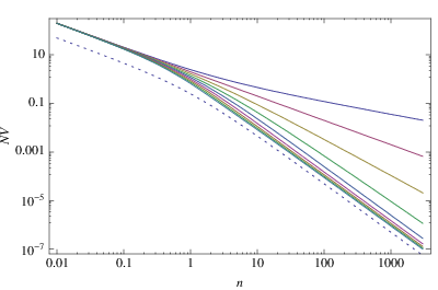
Eq. (26) enables us to compute the Holevo variance in a very efficient way for arbitrary values of $N$ and $n$. Fig. 1 shows a log-log plot of $NV$ against $n$ for $1\leq N\leq 9$. We see that for low $n$ all curves have the same slope, while for large $n$, as we anticipated in the introduction, the slopes increase up to $N=4$ and then stabilize. We next proceed to calculate these two scalings analytically.

III.1 Large squeezing

For very energetic SVS, $n\gg 1$ $(\beta\rightarrow 1)$, the phase can be estimated with arbitrary accuracy; $\lim_{\beta\rightarrow 1}F=1$. In this regime the crucial issue is to know the rate at which perfect estimation is achieved. For the sake of readability the technical details of the calculation are collected in Appendix A. In this section we only summarize and comment the main results. From Eqs. (A) and (23) one readily sees that the statistical variance at leading order in $1/n$ is

$$(\Delta\hat{\theta})^{2}=\left\{\begin{array}[]{ll}\displaystyle{\xi_{N}\over 2n^{N/2}}&(N\leq 3)\\[10.00002pt] \displaystyle{(1/8)\log n+\xi_{4}\over 2n^{2}}&(N=4)\\[10.00002pt] \displaystyle{1\over 8(N-4)n^{2}}&(N\geq 5),\end{array}\right.$$

where the values of $\xi_{N}$ are given in Table 1. We recall that these statistical variances are obtained assuming that one can perform the most general (collective) measurement on the $N$-copy state $\rho_{\theta}^{\otimes N}$. We find it remarkable that the $n^{-2}$ scaling is only achieved for $N\geq 5$ (see Fig. 1).

$N$	1	2	3	4
$\xi_{N}$	$\ 0.55\$	$\ 1/2\$	$\ 0.58\$	$\ 0.30\$

Table 1: Values of the coefficients $\xi_{N}$ in Eq. (III.1).

Notice that for a single copy, the optimal scaling is $n^{-1/2}$, as compared to $n^{-2}$, which one would naively expect from HL. This scaling is even worse than that attained with coherent states $n^{-1}$ [see Eq. (6)]. The same $n^{-1/2}$ scaling shows up in the $n$-photon two mode state discussed in [25].

Figure 1: Log-log plot of the scaled phase variance $NV$ defined in Eq. (21) for $N$ copies of SVS, $1\leq N\leq 9$ (top to bottom), as a function of the mean photon number $n$ (solid lines). For large $n$ the lines become steeper as $N$ increases, in agreement with Eq. (III.1). The slopes stabilize for $N\geq 5$. For small $n$ the slopes are independent of $N$, as Eqs. (31) and (39) show. The dotted line is the limiting curve ($N\rightarrow\infty$) for both small and large $n$. It follows from the HL (39), as discussed in Sec. V.

Using our analysis we can also study the optimal splitting of energy among copies. If one has a fixed, but large, amount of energy $E$ that can be divided among $N$ copies, each with mean photon number $n=E/N$, it is straightforward to obtain from Eq. (III.1) that asymptotically the optimal choice is $N=8$. This result is also clear from Fig. 2.

Figure 2: Log-log plot of the rescaled phase variance $E^{2}V$ as a function of the total available energy $E=nN$ (in units of $\hbar\omega$). The thin solid lines correspond (from top to bottom) to $N=5,6,7$; the thick green line to $N=8$. Dashed lines correspond to $N\geq 9$ in increasing order from bottom to top on the right side of the plot. For large $E$, variances scale as $E^{-2}$ (all lines have horizontal asymptotes) and $N=8$ clearly provides the smallest variance.

III.2 Small squeezing

Let us now briefly focus on the low energy regime. This regime may be relevant in practical situations where the amount of squeezing is bounded by technological limitations. For $\beta\ll 1$ we have $\beta\simeq\sqrt{n}$ and we can easily find the leading behavior of $F$ by keeping the first terms in Eq. (25). For $nN\ll 1$, a simple calculation gives

$$F\simeq\sqrt{\frac{nN}{2}};\quad V\simeq\frac{2}{nN},$$ (31)

where the approximate expression for $V$ follows from (21) and (22). This shows that the scaling is independent of $N$, as is clear from Fig. 1. Note also that the fidelity only depends on the total energy $E=nN$.

IV Individual measurements: Large $N$

We have shown that the accuracy that can be achieved with a single SVS increases with $n$ at a much lower rate than that inferred from the HL. The natural question that arises is whether the latter can be achieved by performing the same measurement on a large set of identical copies. In other words, we wish to know if the attainability of the HL requires some sort of classical communication between measurers dealing with the various copies. The Fisher information allows to address this question. In single-parameter estimation the Fisher information provides an asymptotic bound (the Cramér-Rao bound) for the accuracy that can be attained by repeating the same measurement on each copy of the sample. Recall that the Fisher information is defined as [28]

$$I(\theta)=\int d\phi~p(\phi|\theta)\left(\frac{\partial\log p(\phi|\theta)}{\partial\theta}\right)^{2},$$ (32)

where $p(\phi|\theta)$ is the conditional probability of obtaining the outcome $\phi$ upon measuring on the state $|\psi_{\theta}\rangle$ that carries a phase $\theta$ . In our case the measurement is defined by Eq. (24) and the corresponding outcome probabilities are

$$p(\phi|\theta)=|S(\phi-\theta)|^{2},$$ (33)

where

$$S(\phi)=\left(\frac{1-\beta^{2}}{\pi^{2}}\right)^{1/4}\sum_{k}\frac{\sqrt{(2k)!}}{k!}\left(\frac{\beta e^{2i\phi}}{2}\right)^{k}.$$ (34)

The covariance of the measurement (24) implies that the Fisher information is independent of $\theta$, as is apparent from the form of the conditional probability (33). For highly energetic SVS ($\beta\simeq 1$) we get

$$I\simeq{6\over 7(1-\beta)^{2}}\simeq\frac{24}{7}n^{2}+\dots$$ (35)

(we refer to Appendix B for details), and by using the Cramér-Rao bound $N(\Delta\hat{\theta})^{2}\geq I^{-1}$, we obtain

$$(\Delta\hat{\theta})^{2}\geq\frac{7}{24}\frac{1}{n^{2}N}.$$ (36)

Recall that this bound is attainable for a large sample, $N\to\infty$, with, e.g., a Bayesian or maximum likelihood estimator [18].

Hence, we obtain that the optimal measurement performed sequentially on a large sample of identically prepared SVS gives an accuracy that scales as the HL, a result that could not easily be anticipated. Notice, however, that the coefficient of the variance is more than a factor of two larger than that of the HL (7/24 as compared to 1/8). This means that in order to obtain the optimal accuracy we may require classical communication [14], i.e., adaptivity of the measurements.

V Discussion

From Eq. (III.1) and Fig. 1 we see that the HL, which predicts a scaling $n^{-2}$ for the variance, is only achieved for $N\geq 5$. Had we naively extrapolated the scaling $n^{-N/2}$ for $N\leq 4$, we would have predicted a breakdown of the HL (see Appendix A). Of course, this is not the case: for $N>4$ the terms with the dangerous exponent behavior in Eq. (46) become sub-dominant in the large $n$ limit, and the statistical variance scales as dictated by the HL.

We can also obtain the exact dependence in the mean number of photons for large $N$. The easiest way is to rewrite $h_{k}h_{k+1}$ in Eq. (25) as $h_{k}^{2}\sqrt{(N/2+k)/(k+1)}$, so that

$$F=\beta\sum_{k=0}^{\infty}\wp_{k}\sqrt{\frac{N/2+k}{k+1}},$$ (37)

where the negative binomial probability distribution $\wp_{k}$ is defined in Eq. (20). To compute this expectation value we expand the square root around the mean of the distribution, $\langle k\rangle=(N/2)\beta^{2}/(1-\beta^{2})$, up to second order. By recalling that $(\Delta k)^{2}=\langle k\rangle/(1-\beta^{2})$, it is straightforward to obtain

$$F=1-\frac{(\beta^{2}-1)^{2}}{4\beta^{2}N},$$ (38)

or equivalently

$$(\Delta\hat{\theta})^{2}=\frac{1}{8n(n+1)N},$$ (39)

which is the exact expression of the HL (see [26, 14] and references therein).

Our results have a number of implications both of fundamental and of practical interest. In the high energy regime they show that, somewhat unexpectedly, the phase resolution of a single squeezed vacuum state is worse than that of a coherent state with the same energy. Our results indicate that whenever a phase measurement is to be performed through interaction with a single copy (or mode) of the probe, one is better off using coherent states. This scenario changes significantly as one moves to the multi-copy case. For two copies the resolution is already comparable to that of coherent states and the variance reaches the HL scaling ($n^{-2}$) for $N>4$. It is important to notice that we have considered arbitrary collective measurements and, hence, our results give the ultimate precision bounds allowed by quantum mechanics. In addition, our analysis provides the means to determine the optimal energy splitting among copies, showing that for highly energetic SVS, the optimal choice is $N=8$, as shown in Fig. 2.

In the low energy regime we have shown that the variance (fidelity) is only a function of the total available energy, regardless the way it splits among copies. This is relevant for practical implementations of squeezed state metrology, where usually the amount of available squeezing is small.

We have also analyzed the asymptotic accuracy of Holevo’s canonical phase measurement (24) when it is performed on each copy of the sample. It gives rise to a scaling of the variance which agrees with the HL of SVS up to a constant multiplicative factor of the order of two. In some sense, this result relaxes the need for adaptive protocols at the expense of having an asymptotic rate that is roughly a half that of the optimal protocol. This shows that individual non-adaptive measurements can harness the enhanced phase variance offered by SVS.

VI Acknowledgments

We are grateful to A. Acín, J. Calsamiglia, M. Mitchell and M.B. Plenio for very useful discussions, and to D. Diego, for contributing to the very early stages of this work. We acknowledge financial support from the Spanish MCyT, CONSOLIDER2006-00019 and FIS2005-01369, and CIRIT 2005SGR-00994. A.M. also acknowledges financial support from QIP IRC GR/S82176/01.

Appendix A Calculation of $F$ for SVS

In this Appendix we provide details of our calculation of the fidelity for SVS. Our starting point is Eq. (25). Taking into account Eq. (18) we can write

$$F\leq(1-\beta^{2})^{N/2}\sum_{k=0}^{\infty}\frac{\beta^{2k+1}c_{k}}{\sqrt{(k+1)(k+N/2)}},$$ (40)

where we have defined

$$c_{k}=\frac{N}{2}\binom{k+N/2}{k}.$$ (41)

We next apply the integral representation (9) to both $(k+1)^{-1/2}$ and $(k+N/2)^{-1/2}$,

$$\frac{1}{\sqrt{(k+1)(k+N/2)}}=\\ \int_{0}^{\infty}\int_{0}^{\infty}dt_{1}dt_{2}\frac{\exp[-(k+1)t_{1}-(k+N/2)t_{2}]}{\pi\sqrt{t_{1}t_{2}}}.$$ (42)

This enables us to sum up the series (over $k$) in (40) by recalling the negative binomial expansion $\sum_{k}c_{k}z^{k}=(N/2)(1-z)^{-N/2-1}$. We are left with a double integral, which can be further simplified by the change of variables $(t_{1},t_{2})\rightarrow(u,\tau)$:

$$t_{1} = -u\log\left(\tfrac{1-\tau}{\beta^{2}}\right),$$ (43)

$$t_{2} = -(1-u)\log\left(\tfrac{1-\tau}{\beta^{2}}\right),$$ (44)

and by recalling the integral representation of the zero order modified Bessel function of the first kind [24]

$$I_{0}(x)=\frac{1}{\pi}\int_{0}^{1}du\frac{e^{(1-2u)x}}{\sqrt{u(1-u)}}.$$ (45)

The remaining integral can be cast as

$$F=\frac{N}{2}\beta(1-\beta^{2})^{N/2}\int_{1-\beta^{2}}^{1}\frac{g(\tau,\beta)}{\tau^{1+N/2}}d\tau,$$ (46)

where

$$g(\tau,\beta)=\frac{1}{1-\tau}\left(\frac{1-\tau}{\beta^{2}}\right)^{\frac{2+N}{4}}I_{0}\left(\tfrac{2-N}{4}\log\tfrac{1-\tau}{\beta^{2}}\right).$$ (47)

Eqs. (46) and (47) provide a very useful expression of $F$. The integral over $\tau$ can be computed to arbitrary accuracy and it is valid for any number of copies and for any average photon number. It allows, e.g., to find out the optimal splitting of the available energy $E$ among copies for phase estimation (see Sec. III.1 and Fig. 2).

We next derive from (46) the high energy scaling of the fidelity. Let us first introduce some short-hand notation. By $\mathcal{N}(\beta)$, we denote the prefactor in (46),

$$\mathcal{N}(\beta)=\frac{N}{2}\beta(1-\beta^{2})^{N/2},$$ (48)

and notice that it is of order $n^{-N/2}$. We further define $S_{P}(\tau,\beta)=\sum_{k=0}^{P}G_{k}(\beta)\tau^{k}$ to be the truncated Taylor expansion of $g(\tau,\beta)$ around $\tau=0$ up to order $P$. One can easily check that its corresponding integral over $\tau$,

$$\mathcal{G}_{1}(\beta)=\int_{1-\beta^{2}}^{1}\frac{S_{[N/2]}(\tau,\beta)}{\tau^{1+N/2}}d\tau,$$ (49)

is of order $n^{N/2}$ ($[x]$ is the integer part of $x$), whereas the integral of the remainder,

$$\mathcal{G}_{2}(\beta)=\int_{1-\beta^{2}}^{1}\frac{g(\tau,\beta)-S_{[N/2]}(\tau,\beta)}{\tau^{1+N/2}}d\tau,$$ (50)

is of order $n^{0}$. The leading contribution can be computed by taking the limit $\beta\rightarrow 1$ in $\mathcal{G}_{2}$. Thus, up to subleading order, we have

$$F=\mathcal{N}(\beta)\left[\mathcal{G}_{1}(\beta)+\mathcal{G}_{2}(1)\right].$$ (51)

We next expand the first term, $\mathcal{N}(\beta)\mathcal{G}_{1}(\beta)$, in (51) in powers of $n^{-1/2}$. This expansion provides the leading order contribution to the fidelity (the unity), a subleading term of order $n^{-2}$, which becomes dominant only for $N>4$, and a series of inverse power contributions starting at order $n^{-N/2}$. These latter become irrelevant if $N>4$. On the other hand, the second term, $\mathcal{N}(\beta)\mathcal{G}_{2}(1)$, results in corrections of order $n^{-N/2}$ which contribute to the subleading order if $N\leq 4$ and become irrelevant otherwise (of order smaller than $n^{-2}$).

In summary, we have

$$F=1-\left\{\begin{array}[]{ll}\displaystyle{\xi_{N}\over n^{N/2}}&(N\leq 3)\\[10.00002pt] \displaystyle{(1/8)\log n+\xi_{4}\over n^{2}}&(N=4)\\[10.00002pt] \displaystyle{1\over 4(N-4)n^{2}}&(N\geq 5),\end{array}\right.$$

where $\xi_{N}$ are formally defined in terms of definite integrals. Its numerical values are given in Table I. The exact value $\xi_{2}=1/2$ can be trivially obtained from Eq. (37), which yields $F=\beta$.

Appendix B Phase estimation with individual measurements

In this Appendix we compute the Fisher information of the optimal 1-copy measurement. This leads to the Cramér-Rao bound discussed in section IV.

We first notice that the dominant behavior of $S(\theta)$ in Eq. (34) is determined by the asymptotic expressions of the factorials in the sum. The Stirling approximation gives

$$S(\phi) \simeq \left(\frac{1-\beta^{2}}{\pi^{2}}\right)^{1/4}\frac{1}{\pi^{1/4}}\sum_{k}\frac{(\beta e^{2i\phi})^{k}}{k^{1/4}}$$ (56)

$$= \left(\frac{1-\beta^{2}}{\pi^{2}}\right)^{1/4}\frac{\mathrm{Li}_{1/4}(\beta e^{2i\phi})}{\pi^{1/4}},$$

where $\mathrm{Li}_{s}(z)=\sum_{k=1}^{\infty}z^{k}/k^{s}$ is the polylogarithm function of order $s$ [24]. Since we are only interested in the asymptotic behavior for large squeezing ($\beta\to 1$), we can use the first order expansion around $z=1$, which reads $\mathrm{Li_{1/4}}(z)=\Gamma(3/4)(1-z)^{-3/4}+\dots$ [24]. We note in passing that the probability law obtained by retaining only this term is consistent with the normalization condition, i.e., $\int p(\phi|\theta)d\phi\to 1$ when $\beta\to 1$. In this limit we can easily compute the derivatives required in (32) and obtain

$$I\simeq\frac{9\Gamma(\frac{3}{4})^{2}\sqrt{1-\beta^{2}}}{\pi^{3/2}}\int_{-\frac{\pi}{2}}^{\frac{\pi}{2}}\!\frac{d\phi\,\sin^{2}2\phi}{(1-2\beta\cos 2\phi+\beta^{2})^{\frac{11}{4}}}\,,$$ (57)

where we have used the rotational invariance of the integral. Notice that the Fisher information is independent of the phase of $|\psi_{\theta}\rangle$. This is just a consequence of the continuous and covariant character of the measurement (7) and the isotropy of the prior. Again, in the limit $\beta\to 1$ the main contribution to the integral is peaked around $\phi\to 0$ and we can Taylor-expand the trigonometric functions and safely extend the integration limits from $(-\pi/2,\pi/2)$ to $(-\infty,\infty)$. We thus obtain

$$\kern-30.00005ptI\simeq\frac{36\Gamma^{2}(\frac{3}{4})\beta^{2}\sqrt{1-\beta^{2}}}{\pi^{3/2}}\int_{-\infty}^{\infty}\frac{d\phi\,\phi^{2}}{[(1-\beta)^{2}+4\beta\phi^{2}]^{\frac{11}{4}}}$$

$$\kern-30.00005pt\phantom{I}=\frac{3}{7}\frac{\sqrt{2\beta(1+\beta)}}{(1-\beta)^{2}}\simeq\frac{6}{7(1-\beta)^{2}}.$$ (58)

This is the Fisher information used in Eq. (35) in the main text.

References

- [1] C.H. Bachor, A guide to Experiments in Quantum Optics, (Willey-VCH, Weinheim 1998).
- [2] M. Xiao, L.-A. Wu and H.J. Kimble, Phys. Rev. Lett. 59, 278 (1987).
- [3] M.I. Kobolov and C. Fabre, Phys. Rev. Lett. 85, 3789 (2000).
- [4] C.M. Caves, Phys. Rev. D 23, 1693 (1981).
- [5] N. Treps et al., Science 301, 940 (2003).
- [6] C. Fabre, J.B. Fouet and A. Maître, Opt. Lett. 25, 76 (2000).
- [7] N. Treps et al., Phys. Rev. Lett. 88, 203601 (2002).
- [8] H.J. Kimble, Y. Levin, A.B. Matsko, K.S. Thorne and S.P. Vyatchanin, Phys. Rev. D 65, 022002 (2002).
- [9] B. Abbott et al., Nucl. Instrum. Methods 517, 154 (2004).
- [10] H. Vahlbruch et al., Phys. Rev. Lett. 97, 011101 (2006).
- [11] M.D. Lukin, S.F. Yelin, and M. Fleischhauer, Phys. Rev. Lett. 84, 4232 (2000).
- [12] V. Petersen and L.B. Madsen and K. Molmer, Phys. Rev. A 71, 012312 (2005).
- [13] C. Monroe, Nature 416, 238 (2002).
- [14] A. Monras, Phys. Rev. A 73, 033821 (2006).
- [15] A.S. Holevo, Lect. Notes Math. 1055, 153 (1984)
- [16] A.S. Holevo, Quantum Probability and Applications to the Quantum Theory of Irreversible Processes, Springer Lecture Notes in Mathematics, Vol. 1055, p.153 (Springer-Verlag, Berlin, 1984).
- [17] H. Cramér, Mathematical Methods of Statistics (Princeton University Press, Princeton, 1946)
- [18] S.L. Braunstein and C.M. Caves, Phys. Rev. Lett. 72, 3439 (1994).
- [19] V. Giovannetti, S. Lloyd and L. Maccone, Phys. Rev. Lett. 96, 010401 (2006).
- [20] S. Boixo, S.T. Flammia, C.M. Caves and J.M. Geremia, Phys. Rev. Lett. 98, 090401 (2007); S. Boixo, A. Datta, S.T. Flammia, A. Shaji, E. Bagan and C.M. Caves, Phys. Rev. A 77, 012317 (2008).
- [21] W.P. Schelich and S.M. Barnett, Special Issue of Phys. Scr. T48 (1993).
- [22] E. Bagan, A. Monras and R. Munoz-Tapia, Phys. Rev. A 71, 062318 (2005).
- [23] H.M. Wiseman and R.B. Killip, Phys. Rev. A 56, 944 (1997); H.M. Wiseman and R.B. Killip, Phys. Rev. A 57, 2169 (1998).
- [24] M. Abramowitz and I.A. Stegun, Handbook of Mathematical Functions (Dover, New York, 1970).
- [25] D.W. Berry and H.M. Wiseman, Phys. Rev. Lett. 85, 5098 (2000).
- [26] B. Yurke, S.L. McCall, and J.R. Klauder, Phys. Rev. A 33, 4033 (1987).
- [27] D. Stirzaker, Elementary Probability (Cambridge University Press, Cambridge, 1994).
- [28] T.M. Cover and J.A. Thomas, Elements of Information Theory (Wiley Series in Telecommunications, John Wiley & Sons, New York, 1991).