MPP–2008–65
Finite baryon and isospin chemical potential in AdS/CFT with flavor

Abstract

We investigate the thermodynamics of a thermal field theory in presence of both a baryon and an isospin chemical potential. For this we consider a probe of several D$7$-branes embedded in the AdS-Schwarzschild black hole background.

We determine the structure of the phase diagram and calculate the relevant thermodynamical quantities both in the canonical and in the grand canonical ensemble. We discuss how accidental symmetries present reflect themselves in the phase diagram: In the case of two flavors, for small densities, there is a rotational symmetry in the plane spanned by the baryon and isospin density which breaks down at large densities, leaving a $\mathbb{Z}_{4}$ symmetry.

Finally, we calculate vector mode spectral functions and determine their dependence on either the baryon or the isospin density. For large densities, a new excitation forms with energy below the known supersymmetric spectrum. Increasing the density further, this excitation becomes unstable. We speculate that this instability indicates a new phase of condensed mesons.

1 Introduction

Generalizations of the AdS/CFT correspondence [1, 2] have proven to be very useful in describing strongly coupled QCD-like theories. In particular, the AdS-Schwarzschild black hole background provides a gravity dual for four-dimensional $\mathcal{N}=4$ $SU(N)$ SYM theory at finite temperature [3]. This is expected to be relevant for describing some aspects of the strongly coupled quark-gluon plasma. Hydrodynamic methods based on gauge/gravity duality have been applied very successfully to describing transport processes [4, 5, 6, 7, 8, 9, 10, 11, 12, 13, 14, 15, 16, 17, 18, 19, 20, 21].

A further important ingredient for obtaining gravity duals of field theories similar to QCD is the addition of flavor degrees of freedom via the embedding of D$7$-brane probes [22]. A D$7$-brane probe embedded in the AdS Schwarzschild background displays an interesting first-order phase transition between embeddings which do not reach the black hole horizon and those who do [23, 24, 25, 26]. The first kind of embeddings is often said to be a “Minkowski embedding” while the second is called a “black hole embedding”. The phase diagram is modified in presence of a $U(1)$ baryon chemical potential given by a non-zero vev for the time component of the gauge field on the brane [27, 28, 29, 30]. The effect of a finite baryon chemical potential is also studied in the $dS_{4}$ background, e. g. [31], and in the Sakai-Sugimoto model, e. g. [32, 33].

The spectral functions for the D$7$ system, calculated according to the holographic prescription of [34, 35], also display a rich structure, as investigated for instance in [36, 37, 38, 39, 40, 41, 42]. In particular, as shown in [43], in presence of a baryon chemical potential, the vector quasiparticle resonances approach the supersymmetric meson mass spectrum of [44] for large values of the quark mass or small values of the temperature. At small values of the quark mass or large values of the temperature, the frequencies of the resonance peaks increase with rising temperature. Moreover it was shown in [43] that in presence of an $SU(2)$ isospin chemical potential given by a non-zero vev for the time component of the gauge field on a probe of two coincident D$7$-branes, the vector spectral function displays a triplet splitting of the resonance peaks.

In the present paper we determine the structure of the phase diagram in presence of both a $U(1)$ baryon and an $SU(2)$ isospin chemical potential, of the form

$$\mu=\mu^{B}\left(\begin{array}[]{cc}1&0\\ 0&1\end{array}\right)+\mu^{I}\left(\begin{array}[]{cc}1&0\\ 0&-1\end{array}\right).$$ (1.1)

We thus restrict ourselves to an isospin chemical potential in the $\sigma^{3}$ direction in flavor space. This restriction was suggested and used also in [45]. The values of $\mu^{B}$ and $\mu^{I}$ are given in terms of fields which depend on the holographic radial direction. Some features of this setup are generalized to a general small number $N_{f}\ll N_{c}$ of flavor probe branes. For the discussion of the phase structure we restrict to $N_{f}=2$.

Using a suitable linear combination of the flavor components, the action determining the brane embedding splits into a sum of Abelian contributions. Moreover the choice of (1.1) leads to a number of accidental symmetries which we list in detail. We discuss the case of arbitrary $N_{f}$ as well as $N_{f}=2$. In addition to a reflection and a permutation symmetry, there is also an approximate $O(N_{f})$ symmetry if the baryonic and isospin densities, parametrized by $\tilde{d}^{B}$ and $\tilde{d}^{I}$, are small.

We investigate the phase diagram and calculate thermodynamic quantities such as the free energy (grand potential), entropy, energy and speed of sound in the canonical (grand canonical) ensemble. Generically, a special case arises when the normalized baryon and isospin densities coincide, $d^{I}=d^{B}$. The relation $|d^{I}|=|d^{B}|$ determines fixed lines of the permutation and reflection symmetry transformations.

In the canonical ensemble at vanishing isospin density, there is a phase transition between black hole embeddings below a critical baryon density [27]. At both finite baryon and isospin density, the according critical point becomes a critical line which displays the approximate $O(2)$ symmetry up to a small derivation which we quantify. We proceed by investigating a new first order phase transition in the density plane in the limit of large quark mass over temperature ratio. The phase diagram clearly displays the symmetry fixed lines $|d^{I}|=|d^{B}|$ at which the chemical potentials develop a discontinuous gap, which marks the first order phase transition. This is similar to what is observed in two-color QCD [46, fig. 1]. In the four different regions of the phase diagram, the larger of the two densities measures the degrees of freedom in our setup and contributes linearly to the free energy. The smaller density contributes nonlinearly and may be interpreted as a electrostatic-like charge induced by the non-Abelian charges of the quarks.

In the grand canonical ensemble, the sum $\mu^{B}+\mu^{I}$ is relevant. For $\mu^{B}+\mu^{I}<M_{q}$ there is a black hole/Minkowski phase transition which is absent for $\mu^{B}+\mu^{I}>M_{q}$, with $M_{q}$ the bare quark mass. As we discuss in detail, a new phase becomes visible in the grand canonical phase diagram. This is related to the fact that it is not possible to find a bijective map between the canonical and the grand canonical ensemble in the limit of large mass over temperature ratio and of chemical potentials of the order of the quark mass. This implies an instability, e. g. [47, chap. 3].

This motivates us to calculate the spectral function for the gauge field fluctuations in the canonical ensemble at either finite baryon or finite isospin particle density. We identify resonance peaks of the spectral functions with mesonic quasiparticles. For finite baryon density, it was shown in [43] that for $\mu^{B}\approx M_{c}$, with $M_{c}$ the renormalized quark mass in the plasma, the spectrum of these particles approaches the supersymmetric spectrum $M_{n}/(2\pi T)=m\sqrt{(n+1)(n+2)/2}$, with $m=2M_{q}/(\sqrt{\lambda}T)$ found in [44]. The quasiparticle resonances become very narrow in this case. Here, however, we investigate the case of large baryon density and find that these resonances become wide, i. e. unstable, in this limit.

In the case of finite isospin density, we additionally find a new excitation. This new resonance develops at an energy below $M=2\pi Tm$. The new resonance becomes the lowest vector mesonic excitation of the system. It becomes unstable at a critical isospin chemical potential. We interpret this as vector meson condensation, similar to [48]. Moreover we discuss the structure of the phase diagram in $(\mu^{I},M_{q}/T)$ and identify the new phase. We relate the appearance of this phase to the instability discussed above.

We also calculate the effective baryon diffusion coefficient $D$ within hydrodynamics from the membrane paradigm. We find that $D$ displays the hydrodynamic crossover reminiscent of the phase transition present at small densities. The position of the crossover displays a $\mathbb{Z}_{4}$ symmetry in the $(d^{B},d^{I})$-plane.

The paper is organized as follows. In section 2 we introduce the setup of probe D$7$-branes in presence of both a baryon and an isospin chemical potential, paying particular attention to the accidental symmetries. We obtain numerical results for the chemical potentials and the condensate as functions of the quark mass. In section 3 we study the phase diagram and thermodynamic quantities such as free energy, entropy and energy in the canonical ensemble. In section 4 we perform a similar analysis in the grand canonical ensemble, revealing the possibility of an instability. The hydrodynamic diffusion constant is studied in section 5. In section 6 we study the spectral functions of mesonic quasiparticle resonances. For large isospin chemical potentials, we find an instability and identify the corresponding region in the phase diagram.

2 Holographic setup

2.1 Background and brane configuration

We consider asymptotically $AdS_{5}\times S^{5}$ space-time. The $AdS_{5}\times S^{5}$ geometry is holographically dual to the ${\cal N}=4$ super-Yang-Mills theory with gauge group $SU(N_{c})$. The dual description of a finite temperature field theory is an AdS black hole. We use the coordinates of [27] to write the AdS black hole background in Minkowski signature as

$$ds^{2}=\frac{1}{2}\left(\frac{\varrho}{R}\right)^{2}\left(-\frac{f^{2}}{\tilde{f}}\mathrm{d}t^{2}+\tilde{f}\mathrm{d}\vec{x}^{2}\right)+\left(\frac{R}{\varrho}\right)^{2}(\mathrm{d}\varrho^{2}+\varrho^{2}\mathrm{d}\Omega_{5}^{2})\,,$$ (2.1)

with $\mathrm{d}\Omega_{5}^{2}$ the metric of the unit 5-sphere and

$$f(\varrho)=1-\frac{\varrho_{H}^{4}}{\varrho^{4}},\quad\tilde{f}(\varrho)=1+\frac{\varrho_{H}^{4}}{\varrho^{4}}\,,$$ (2.2)

where $R$ is the AdS radius, with

$$R^{4}=4\pi g_{s}N_{c}\,{\alpha^{\prime}}^{2}=2\lambda\,{\alpha^{\prime}}^{2}\,.$$ (2.3)

The temperature of the black hole given by (2.1) may be determined by demanding regularity of the Euclidean section. It is given by

$$T=\frac{\varrho_{H}}{\pi R^{2}}\,.$$ (2.4)

In the following we may use the dimensionless coordinate $\rho=\varrho/\varrho_{H}$, which covers the range from the event horizon at $\rho=1$ to the boundary of the AdS space at $\rho\to\infty$.

To include fundamental matter, we embed $N_{f}$ coinciding D$7$-branes into the ten-dimensional space-time. These D$7$-branes host flavor gauge fields $A_{\mu}$ with gauge group $U(N_{f})$. To write down the DBI action for the D$7$-branes, we introduce spherical coordinates $\{r,\Omega_{3}\}$ in the 4567-directions and polar coordinates $\{L,\phi\}$ in the 89-directions [27]. The angle between these two spaces is denoted by $\theta$ ($0\leq\theta\leq\pi/2$). The six-dimensional space in the $456789$-directions is given by

$$\begin{split}\mathrm{d}\varrho^{2}+\varrho^{2}\mathrm{d}\Omega_{5}^{2}=&\,\mathrm{d}r^{2}+r^{2}\mathrm{d}\Omega_{3}^{2}+\mathrm{d}L^{2}+L^{2}\mathrm{d}\phi^{2}\\ =&\,\mathrm{d}\varrho^{2}+\varrho^{2}(\mathrm{d}\theta^{2}+\cos^{2}\theta\mathrm{d}\phi^{2}+\sin^{2}\theta\mathrm{d}\Omega_{3}^{2})\,,\end{split}$$ (2.5)

where $r=\varrho\sin\theta$, $\varrho^{2}=r^{2}+L^{2}$ and $L=\varrho\cos\theta$. Due to the symmetry, the embedding of the D$7$-branes only depends on the radial coordinate $\rho$. Defining $\chi=\cos\theta$, we parametrize the embedding by $\chi=\chi(\rho)$ and choose $\phi=0$ using the $O(2)$ symmetry in the 89-direction. The induced metric $G$ on the D$7$-brane probes is then

$$ds^{2}(G)=\frac{\varrho^{2}}{2R^{2}}\left(-\frac{f^{2}}{\tilde{f}}\mathrm{d}t^{2}+\tilde{f}\mathrm{d}\vec{x}^{2}\right)+\frac{R^{2}}{\varrho^{2}}\frac{1-\chi^{2}+\varrho^{2}(\partial_{\varrho}\chi)^{2}}{1-\chi^{2}}\mathrm{d}\varrho^{2}+R^{2}(1-\chi^{2})\mathrm{d}\Omega_{3}^{2}\,.$$ (2.6)

The square root of the determinant of $G$ is given by

$$\sqrt{-G}=\frac{\sqrt{h_{3}}}{4}\varrho^{3}f\tilde{f}(1-\chi^{2})\sqrt{1-\chi^{2}+\varrho^{2}(\partial_{\varrho}\chi)^{2}}\,,$$ (2.7)

where $h_{3}$ is the determinant of the 3-sphere metric. The embedding function $\chi$ will be determined numerically in section 2.3.3. It depends on the baryon and isospin chemical potentials we introduce next.

2.2 Introducing baryon and isospin chemical potentials

We introduce baryon and isospin chemical potential as a non-vanishing time component of the non-Abelian background gauge field living on the D$7$-branes [27],

$$\mu=\lim_{\rho\to\infty}A_{0}(\rho)\,.$$ (2.8)

First we consider the case of two different flavors, $N_{f}=2$. The generators of the gauge group $U(N_{f}=2)$ can be chosen as the three Pauli matrices $\sigma^{a}$ completed with the identity $\sigma^{0}$,

$$\sigma^{0}=\begin{pmatrix}1&0\\ 0&1\end{pmatrix}\,,\quad\sigma^{1}=\begin{pmatrix}0&1\\ 1&0\end{pmatrix}\,,\quad\sigma^{2}=\begin{pmatrix}0&-{\mathrm{i}}\\ {\mathrm{i}}&0\end{pmatrix}\,,\quad\sigma^{3}=\begin{pmatrix}1&0\\ 0&-1\end{pmatrix}\,.$$ (2.9)

For simplicity, we only consider the diagonal representations of the gauge group. This is equivalent to rotating the flavor coordinates until our chemical potential lies in the third isospin direction. Thus, the field strength tensor $F^{N_{f}}=\mathrm{d}A^{N_{f}}+A^{N_{f}}\wedge A^{N_{f}}$ on the D$7$-branes may be written as

$$F^{N_{f}=2}_{\mu\nu}=F^{B}_{\mu\nu}\sigma^{0}+F^{I}_{\mu\nu}\sigma^{3}\,.$$ (2.10)

The part of the field strength $F^{B}\sigma^{0}$ corresponding to the $U(1)$ gauge group charges the branes equally and therefore induces a baryon chemical potential [27]. However, the part $F^{I}\sigma^{3}$ corresponding to the $SU(2)$ gauge group charges the branes differently inducing a isospin chemical potential [49, 50]. The definition above may be generalized to arbitrary $N_{f}>2$. Recall that there are $(N_{f}-1)$ diagonal generators of $SU(N_{f})$ which form the Cartan subalgebra. Inspired by the interpretation that a diagonal generator of $SU(N_{f})$ should charge one brane differently with respect to all others, we write the diagonal generators as

$$\lambda^{i}=\mathrm{diag}(1,\dots,\overbrace{-(N_{f}-1)}^{i\text{-th position}},\dots,1)\qquad i=2,\dots,N_{f}\,.$$ (2.11)

For this choice of matrices the first flavor component is treated as the reference quantity. For arbitrary $N_{f}$ the generator of the baryonic part of the gauge group $U(1)$ is called $\lambda^{1}$. Thus, we can generalize (2.10) to

$$F^{N_{f}}_{\mu\nu}=F^{B}_{\mu\nu}\lambda^{1}+\sum_{i=2}^{N_{f}}F^{I_{i}}_{\mu\nu}\lambda^{i}=\sum_{i=1}^{N_{f}}F^{I_{i}}_{\mu\nu}\lambda^{i}$$ (2.12)

where again $F^{B}=F^{I_{1}}$ induces the baryon and $F^{I_{i}}$ for $i\geq 2$ the isospin chemical potential for the $i$-th flavor component. In our setup, the only non-vanishing components of the background field strength are $F_{40}=-F_{04}=\partial_{\rho}A_{0}$ since $A_{0}$ depends on $\rho$ only.

2.3 The DBI action and equations of motion

The DBI action determines the shape of the brane embeddings, i.e. scalar fields $\Phi$, as well as the configuration of gauge fields $A$ on these branes. We consider the case of $N_{f}=2$ coincident D7-branes for which the non-Abelian DBI action reads

$$S_{\text{DBI}}=-T_{D7}\mathrm{Str}\int\!\mathrm{d}^{8}\xi\>\sqrt{\det Q}\sqrt{\det\left(P_{ab}\left[E_{\mu\nu}+E_{\mu i}(Q^{-1}-\delta)^{ij}E_{j\nu}\right]+2\pi\alpha^{\prime}F_{ab}\right)}$$ (2.13)

with

$$Q^{i}{}_{j}=\delta^{i}{}_{j}+{\mathrm{i}}2\pi\alpha^{\prime}[\Phi^{i},\Phi^{k}]E_{kj}\,,$$ (2.14)

where for a D$p$-brane in $d$ dimensions we have $\mu,\,\nu=0,\dots,9$, $a,\,b=0,\dots,p$, $i,\,j=(p+1),\dots,d$, $E_{\mu\nu}=g_{\mu\nu}+B_{\mu\nu}$. In our case we set $p=7$, $d=10$, $B\equiv 0$. The action (2.13) can be simplified significantly by using the spatial and gauge symmetries present in our setup. First we make use of the spatial rotation symmetry in our 8,9-directions in order to rotate to the frame in which $\Phi^{9}\equiv 0$. In this particular frame, all the commutators of our two scalar fields $\Phi^{8},\,\Phi^{9}$ vanish and thus $Q^{i}_{j}=\delta^{i}_{j}$. However, the non-Abelian structure of embeddings and gauge fields is still manifest in the pullback appearing in the action (2.13) as

$$\begin{split}P_{ab}[g_{\mu\nu}]=&g_{ab}+(2\pi\alpha^{\prime})^{2}g_{ij}\left(\partial_{a}\Phi^{i}\partial_{b}\Phi^{j}+{\mathrm{i}}\partial_{a}\Phi^{i}[A_{b},\Phi^{j}]\right.\\ &\left.+{\mathrm{i}}[A_{a},\Phi^{i}]\partial_{b}\Phi^{j}-[A_{a},\Phi^{i}][A_{b},\Phi^{j}]\right)\,.\end{split}$$ (2.15)

The only terms coupling the embeddings $\Phi$ to the gauge fields $A$ are given by the commutator terms in equation (2.15). These commutators vanish due to the following argument. We are free to define the $\tau^{0}$ flavor direction to be the direction parallel to the non-vanishing embedding $\Phi^{8}$ using the $U(1)\subset U(N_{f})$ gauge symmetry. Now we choose our baryonic gauge field to have only a non-vanishing $A_{0}^{0}\mathrm{d}x^{0}\tau^{0}$ component. In the dual field theory, this particular choice corresponds to the case in which the baryon charge representation and the mass representation are simultaneously diagonalizable. A different choice is possible and will most likely change the field theory phenomenology. This applies also to the case of non-coincident D$p$-branes. Finally we use the remaining gauge symmetry $SU(N_{f})\subset U(N_{f})$ in order to restrict to an isospin gauge field $A$ along the third flavor direction only, i.e. $A_{0}^{3}\mathrm{d}x^{0}\tau^{3}$, without loss of generality. Thus the only representations appearing in the background are the diagonal elements $\tau^{0}$ and $\tau^{3}$ of $U(N_{f}=2)$, which constitute the Cartan subalgebra. By definition these representation matrices commute with each other and thus all commutators $[\Phi,A]$ vanish. Therefore all terms coupling the scalars $\Phi$ to the gauge fields $A$ vanish, such that their equations of motion decouple as well. In this way we can consistently truncate the non-Abelian DBI action to

$$\begin{split}S_{\text{DBI}}&=-T_{D7}\int\!\mathrm{d}^{8}\xi\;\mathrm{Str}\left(\sqrt{|\det\left(G\sigma^{0}+2\pi\alpha^{\prime}F^{N_{f}=2}\right)|}\right)\\ &=-T_{D7}\int\!\mathrm{d}^{8}\xi\;\sqrt{-G}\,\mathrm{Str}\left(\sqrt{\sigma^{0}+(2\pi\alpha^{\prime})^{2}G^{00}G^{44}\left(F_{40}^{N_{f}=2}\right)^{2}}\right)\,,\end{split}$$ (2.16)

where in the second line the determinant is calculated. Next we determine the square of the non-vanishing components of the field strength tensor, which is by construction diagonal in the flavor space,

$$\begin{split}\left(F_{40}^{N_{f}=2}\right)^{2}&=\left[\left(F^{B}_{40}\right)^{2}+\left(F^{I}_{40}\right)^{2}\right]\sigma^{0}+2F^{B}_{40}F^{I}_{40}\sigma^{3}\\ &=\mathrm{diag}\left\{\left(F^{B}_{40}+F^{I}_{40}\right)^{2},\left(F^{B}_{40}-F^{I}_{40}\right)^{2}\right\}\,,\end{split}$$ (2.17)

where we used $\left(\sigma^{3}\right)^{2}=\sigma^{0}$. Defining the new fields

$$X_{1}=A_{0}^{B}+A_{0}^{I}\qquad\text{and}\qquad X_{2}=A_{0}^{B}-A_{0}^{I}\,,$$ (2.18)

the square of the field strength can be written as

$$\left(F_{40}^{N_{f}=2}\right)^{2}=\mathrm{diag}\left\{\left(\partial_{\rho}X_{1}\right)^{2},\left(\partial_{\rho}X_{2}\right)^{2}\right\}\,.$$ (2.19)

Notice that the field $X_{i}$ is the gauge field living on the $i$-th brane. Inserting the metric components, the action (2.16) becomes

$$\begin{split}S_{\text{DBI}}=-T_{D7}\int&\!\mathrm{d}^{8}\xi\;\frac{\sqrt{h_{3}}}{4}\varrho^{3}f\tilde{f}(1-\chi^{2})\\ \times\Bigg(&\sqrt{1-\chi^{2}+\varrho^{2}(\partial_{\varrho}\chi)^{2}-2(2\pi\alpha^{\prime})^{2}\frac{\tilde{f}}{f^{2}}(1-\chi^{2})(\partial_{\varrho}X_{1})^{2}}\\ &+\sqrt{1-\chi^{2}+\varrho^{2}(\partial_{\varrho}\chi)^{2}-2(2\pi\alpha^{\prime})^{2}\frac{\tilde{f}}{f^{2}}(1-\chi^{2})(\partial_{\varrho}X_{2})^{2}}\Bigg)\,.\end{split}$$ (2.20)

The transformation to the fields $X_{i}$ decouple the two branes and we obtain a sum of two Abelian DBI actions. The Abelian actions are known from the pure baryonic case [27] and we therefore can use the ideas given in the pure baryonic case to study our setup in which baryon and isospin charges are switched on simultaneously.

Now we generalize this result to arbitrary $N_{f}$: Also for this case, we can decouple the non-Abelian gauge field into Abelian gauge fields on each brane. For simplicity we suppress the according index $N_{f}$ on the field strength tensor. We again start from the DBI action for the D$7$-branes,

$$S_{\text{DBI}}=-T_{D7}\int\!\mathrm{d}^{8}\xi\;\mathrm{Str}\left(\sqrt{|\det(G\lambda^{1}+2\pi\alpha^{\prime}F)|}\right)\,.$$ (2.21)

Since this action is diagonal in flavor space, we are able to evaluate the square root and the trace directly (for more details see appendix A). After a redefinition of the fields

$$X_{1}=\sum_{j=1}^{N_{f}}A^{I_{j}}_{0}\,,\qquad X_{i}=\sum_{\begin{subarray}{c}j=1\\ j\not=i\end{subarray}}^{N_{f}}A^{I_{j}}_{0}-(N_{f}-1)A^{I_{i}}_{0}\,,\quad i=2,\dots,N_{f}\,,$$ (2.22)

where $X_{i}$ is the $i$-th flavor component of the gauge field $A^{N_{f}}$, the non-Abelian DBI action again becomes a sum of $N_{f}$ Abelian DBI actions,

$$\begin{split}S_{\text{DBI}}=-T_{D7}\int&\!\mathrm{d}^{8}\xi\;\frac{\sqrt{h_{3}}}{4}\varrho^{3}f\tilde{f}(1-\chi^{2})\\ &\times\sum_{i=1}^{N_{f}}\sqrt{1-\chi^{2}+\varrho^{2}(\partial_{\varrho}\chi)^{2}-2(2\pi\alpha^{\prime})^{2}\frac{\tilde{f}}{f^{2}}(1-\chi^{2})(\partial_{\varrho}X_{i})^{2}}\,.\end{split}$$ (2.23)

Thus we may consider each brane separately with the gauge fields $X_{i}$ treated as a $U(1)$ gauge field living on the $i$-th brane. The action for each brane is the same as the action for the pure baryonic case [27]. In the following we apply the approach of [27]. First we calculate the electric displacement $d_{i}$ on the $i$-th brane, which is a constant of motion and proportional to the flavor charge density,

$$\begin{split}d_{i}=\frac{\delta S_{\text{DBI}}}{\delta(\partial_{\varrho}X_{i})}=&(2\pi\alpha^{\prime})^{2}T_{D7}\sqrt{h_{3}}\varrho^{3}\frac{\tilde{f}^{2}}{2f}\\ &\times\frac{(1-\chi^{2})^{2}\partial_{\varrho}X_{i}}{\sqrt{1-\chi^{2}+\varrho^{2}(\partial_{\varrho}\chi)^{2}-2(2\pi\alpha^{\prime})^{2}\frac{\tilde{f}}{f^{2}}(1-\chi^{2})(\partial_{\varrho}X_{i})^{2}}}\,.\end{split}$$ (2.24)

From the relations of the gauge fields (2.22), we can read off the relations between the conjugate charge densities

$$d^{B}=d^{I_{1}}=\sum_{j=1}^{N_{f}}d_{j}\,,\qquad d^{I_{i}}=\sum_{\begin{subarray}{c}j=1\\ j\not=i\end{subarray}}d_{j}-(N_{f}-1)d_{i}\quad i=2,\dots,N_{f}\,,$$ (2.25)

which for $N_{f}=2$ becomes

$$d^{B}=d_{1}+d_{2}\qquad\text{and}\qquad d^{I}=d_{1}-d_{2}\,.$$ (2.26)

We now construct the Legendre transformation of the action (2.23) to eliminate the fields $X_{i}$ in favor of the constants $d_{i}$,

$$\begin{split}\tilde{S}_{\text{DBI}}&=S_{\text{DBI}}-\int\!\mathrm{d}^{8}\xi\;\sum_{i=1}^{N_{f}}X_{i}\frac{\delta S_{\text{DBI}}}{\delta(\partial_{\varrho}X_{i})}\\ &\begin{split}=-T_{D7}\int\!\mathrm{d}^{8}\xi\;&\frac{\sqrt{h_{3}}}{4}\varrho^{3}f\tilde{f}(1-\chi^{2})\sqrt{1-\chi^{2}+\varrho^{2}(\partial_{\varrho}\chi)^{2}}\\ &\times\sum_{i=1}^{N_{f}}\sqrt{1+\frac{8d_{i}^{2}}{(2\pi\alpha^{\prime})^{2}T_{D7}^{2}\varrho^{6}\tilde{f}^{3}(1-\chi^{2})^{3}}}\,.\end{split}\end{split}$$ (2.27)

The gauge fields can be calculated from the Legendre transformed action by $\partial_{\varrho}X_{i}=-\delta\tilde{S}_{\text{DBI}}/\delta d_{i}$.

It is convenient to introduce the dimensionless quantity

$$\tilde{d}_{i}=\frac{d_{i}}{2\pi\alpha^{\prime}\varrho_{H}^{3}T_{D7}}\,.$$ (2.28)

2.3.1 Accidental symmetries

The DBI action (2.27) has the following discrete symmetries:

Permutation: $d_{i}\leftrightarrow d_{j}$ for $i,j=1,\ldots,N_{f}$ :

Since $d_{i}$ is the electric displacement of the $i$-th brane and the coincident branes have the same embedding function by definition, the substitution $d_{i}\leftrightarrow d_{j}$ interchanges the two branes.

Reflection: $d_{i}\leftrightarrow-d_{i}$ for each $i=1,\dots,N_{f}$ :

We consider an $U(1)$ gauge field with only the time component non-vanishing. Since it does not depend on the time, our setup is like an electrostatic situation. To change the sign of the electric displacement $\tilde{d}_{i}$, we must change the sign of the gauge field $X_{i}$ (see equation (2.24)). The sign change in the gauge field may be induced by a sign change of the electric charge generating the gauge field $X_{i}$, which may be interpreted as an interchange between particle and anti-particle. The symmetry $d_{i}\leftrightarrow-d_{i}$ is therefore induced by the invariance of our system interchanging particles with anti-particles on the $i$-th brane.

If we expand the action (2.27) for small $d_{i}$,

$$\begin{split}\tilde{S}_{\text{DBI}}=-T_{D7}\int\!\mathrm{d}^{8}\xi\;&\frac{\sqrt{h_{3}}}{4}\rho^{3}f\tilde{f}(1-\chi^{2})\sqrt{1-\chi^{2}+\rho^{2}(\partial_{\rho}\chi)^{2}}\\ &\times\left(N_{f}+\frac{8\sum_{i=1}^{N_{f}}d_{i}^{2}}{(2\pi\alpha^{\prime})^{2}T_{D7}\rho^{6}\tilde{f}^{3}(1-\chi^{2})^{3}}+\cdots\right)\,,\end{split}$$ (2.29)

we observe an approximate $O(N_{f})$ symmetry

$$(d_{1},\dots,d_{N_{f}})\leftrightarrow{\cal O}(d_{1},\dots,d_{N_{f}})\,,\quad{\cal O}\in O(N_{f})\,.$$ (2.30)

The approximate $O(N_{f})$ symmetry, which consists of the $SO(N_{f})$ group and reflections, is the continuous symmetry generated by the discrete symmetries since the $SO(N_{f})$ generators are real skew-symmetric matrices which can be represented by reflection and permutation matrices.

In the physical basis the effect of the symmetry transformation above is given by

• $d_{i}\leftrightarrow d_{j}$:

  $$\text{for} i,j\not=1: d^{I_{i}}\leftrightarrow d^{I_{j}}$$ (2.31)

  $$\text{for} i=1,\,j\not=1:\quad d^{B}\leftrightarrow d^{B}\qquad\text{and}\qquad d^{I_{j}}\leftrightarrow-\sum_{k=2}^{N_{f}}d^{I_{k}},$$

• $d_{i}\leftrightarrow-d_{i}$:

  $$d^{I_{i}}\leftrightarrow-d^{I_{i}}+2\sum_{j\not=i}d_{j}\qquad\text{and}\qquad d^{I_{j}}\leftrightarrow d^{I_{j}}-2d_{i}\quad j\not=i\,.$$ (2.32)

For $N_{f}=2$ we get

$$d_{1} \leftrightarrow d_{2}: d^{B}\mapsto d^{B} \text{and} d^{I}\mapsto-d^{I}$$ (2.33)

$$d_{1} \leftrightarrow-d_{1}:\qquad d^{B}\mapsto-d^{I}\qquad \text{and}\qquad d^{I}\mapsto-d^{B}$$

$$d_{2} \leftrightarrow-d_{2}: d^{B}\mapsto d^{I} \text{and} d^{I}\mapsto d^{B}\,.$$

These symmetries are also present in 2-color QCD theories with degenerated quark mass [46]. Since the transformation matrix to the physical basis is proportional to an $O(2)$ matrix, there is also an induced approximate $O(2)$ symmetry in the physical basis. The results for the case $N_{f}=3$ are shown in the appendix B.

2.3.2 Gauge fields

We now determine the gauge fields which will allow us to compute the chemical potentials. Therefore, we write down the asymptotic form of the gauge field close to the boundary,

$$A_{0}^{I_{i}}=\mu^{I_{i}}-\frac{\tilde{d}^{I_{i}}}{2\pi\alpha^{\prime}}\frac{\varrho_{H}}{\rho^{2}}+\cdots\qquad\text{for}\qquad i=1,\ldots,N_{f}\,,$$ (2.34)

where the coefficients $\mu^{I_{i}}$ and $\tilde{d}^{I_{i}}$ are related to the baryon/isospin chemical potential and the baryon/isospin density $n_{q}^{I_{i}}$, respectively,

$$\tilde{d}^{I_{i}}=\frac{2^{\frac{5}{2}}n_{q}^{I_{i}}}{N_{f}N_{c}\sqrt{\lambda}T^{3}}.$$ (2.35)

Obviously, the chemical potential $\mu^{I_{i}}$ depends on the corresponding density $\tilde{d}^{I_{i}}$. To determine, this dependence it is convenient to use the dimensionless quantities

$$\tilde{X}_{i}=\frac{2\pi\alpha^{\prime}}{\varrho_{H}}X_{i}\,,\qquad\tilde{\mu}_{i}=\frac{2\pi\alpha^{\prime}}{\varrho_{H}}\mu_{i}=\sqrt{\frac{2}{\lambda}}\frac{\mu_{i}}{T}\,.$$ (2.36)

As described above, the transformed action (2.27) may be used to calculate the gauge fields and therefore the chemical potentials (see [27] for more details)

$$\tilde{\mu}_{i}=\tilde{X}_{i}(\rho=\infty)=2\tilde{d}_{i}\int_{1}^{\infty}\!\mathrm{d}\rho\;\frac{f\sqrt{1-\chi^{2}+\varrho^{2}(\partial_{\rho}\chi)^{2}}}{\sqrt{\tilde{f}(1-\chi^{2})[\rho^{6}\tilde{f}^{3}(1-\chi^{2})^{3}+8\tilde{d}_{i}^{2}]}}\,.$$ (2.37)

The connection to the physical basis is given by

$$\tilde{\mu}_{1}=\sum_{j=1}^{N_{f}}\tilde{\mu}^{I_{j}}\,,\qquad\tilde{\mu}_{i}=\sum_{j\not=i}\tilde{\mu}^{I_{j}}-(N_{f}-1)\tilde{\mu}^{I_{i}}\quad i=2,\dots,N_{f}\,,$$ (2.38)

which for $N_{f}=2$ becomes

$$\tilde{\mu}^{B}=\frac{1}{2}(\tilde{\mu}_{1}+\tilde{\mu}_{2})\qquad\text{and}\qquad\tilde{\mu}^{I}=\frac{1}{2}(\tilde{\mu}_{1}-\tilde{\mu}_{2})\,.$$ (2.39)

Notice that in the Abelian case [27] it is found that in the limit $m\to\infty$ the chemical potentials $\mu_{i}$ approach $M_{q}$ for positive $\tilde{d}_{i}$. This allows us to calculate the physical chemical potentials in the limit $m\to\infty$,

$$\mu^{B}\to M_{q}\qquad\text{and}\qquad\mu^{I_{i}}\to 0\quad i=2,\ldots,N_{f},$$ (2.40)

if $\tilde{d}_{j}>0$ for $j=1,\ldots,N_{f}$. In the case $\tilde{d}_{i}<0$, using the accidental symmetry of the action $\tilde{d}_{i}\leftrightarrow-\tilde{d}_{i}$ presented in section 2.3.1, we get also a sign change in the chemical potential $\mu_{i}\leftrightarrow-\mu_{i}$. Therefore, if we change the sign of just one $\tilde{d}_{i}$, there is at least one isospin chemical potential $\tilde{\mu}^{I_{i}}$ which does not vanish any more. For $N_{f}=2$ we explicitly get

$$\mu^{B} \to M_{q}\quad \text{and}\quad \mu^{I}\to 0\qquad \text{for }\tilde{d}_{1},\,\tilde{d}_{2}>0 \text{{i.\,e.\ }}\quad 0\leq\tilde{d}^{I}<\tilde{d}^{B}$$ (2.41)

$$\mu^{B} \to 0 \text{and} \mu^{I}\to M_{q} \text{for }-\tilde{d}_{1}<\tilde{d}_{2}<0\quad \text{{i.\,e.\ }}\quad 0\leq\tilde{d}^{B}<\tilde{d}^{I}\,.$$

If we set one density to zero in the case $N_{f}=2$, e. g. $\tilde{d}_{2}=0$, only the first brane is charged. Therefore, the chemical potential $\mu_{1}$ approaches $M_{q}$ and $\mu_{2}$ approaches zero in the limit $m\to\infty$. Using equation (2.39), this implies

$$\mu^{B}\to\frac{M_{q}}{2}\qquad\text{and}\qquad\mu^{I}\to\frac{M_{q}}{2}\qquad\text{for }\tilde{d}_{1}>0,\,\tilde{d}_{2}=0\quad\text{{i.\,e.\ }}\quad 0<\tilde{d}^{B}=\tilde{d}^{I}\,.$$ (2.42)

This discontinuous step suggests that there is a phase transition between the regions $0\leq\tilde{d}^{I}<\tilde{d}^{B}$ and $0\leq\tilde{d}^{B}<\tilde{d}^{I}$. We also expect a similar phase transition for arbitrary $N_{f}$. In section 3.3 we discuss this phase transition further.

2.3.3 Embeddings

The equation of motion for the embedding function $\chi$ can be derived from (2.27) as

$$\begin{split}&\partial_{\rho}\left[\rho^{5}f\tilde{f}(1-\chi^{2})\frac{\partial_{\rho}\chi}{\sqrt{1-\chi^{2}+\rho^{2}(\partial_{\rho}\chi)^{2}}}\sum_{i=1}^{N_{f}}\sqrt{1+\frac{8\tilde{d}_{i}^{2}}{\rho^{6}\tilde{f}^{3}(1-\chi^{2})^{3}}}\right]\\ =&-\frac{\rho^{3}f\tilde{f}\chi}{\sqrt{1-\chi^{2}+\rho^{2}(\partial_{\rho}\chi)^{2}}}\Bigg[\left[3\left(1-\chi^{2}\right)+2\rho^{2}(\partial_{\rho}\chi)^{2}\right]\sum_{i=1}^{N_{f}}\sqrt{1+\frac{8\tilde{d}_{i}^{2}}{\rho^{6}\tilde{f}^{3}(1-\chi^{2})^{3}}}\\ &-\frac{24}{\rho^{6}\tilde{f}^{3}(1-\chi^{2})^{3}}\left(1-\chi^{2}+\rho^{2}(\partial_{\rho}\chi)^{2}\right)\sum_{i=1}^{N_{f}}\frac{\tilde{d}_{i}^{2}}{\sqrt{1+\frac{8\tilde{d}_{i}^{2}}{\rho^{6}\tilde{f}^{3}(1-\chi^{2})^{3}}}}\Bigg]\,.\end{split}$$ (2.43)

In addition to the case without isospin density [27], sums over the $N_{f}$ different densities appear in the equation of motion for the embedding function. Due to these sums, the equation of motion cannot be written down in a more compact form, as done in the Abelian case [27].

To relate the gravity field $\chi$ to the dual gauge field parameters we consider the asymptotic form for the embedding function $\chi$ close to the boundary,

$$\chi=\frac{m}{\rho}+\frac{c}{\rho^{3}}+\cdots\,.$$ (2.44)

Then the AdS/CFT dictionary relates the coefficients $m$ and $c$ to the bare quark mass $M_{q}$ and the quark condensate $\langle\bar{\psi}\psi\rangle$, respectively,

$$m=\frac{2M_{q}}{\sqrt{\lambda}T}\,,\qquad c=-\frac{8\langle\bar{\psi}\psi\rangle}{\sqrt{\lambda}N_{f}N_{c}T^{3}}\,.$$ (2.45)

The initial conditions to solve equation of motion (2.43) numerically are $\chi(\rho=1)=\chi_{0}$ and $\partial_{\rho}\chi(\rho=1)=0$. We determine the parameter $m$ and $c$, which depend on $\chi_{0}$, by fitting the numerical solution to the asymptotic form (2.44).

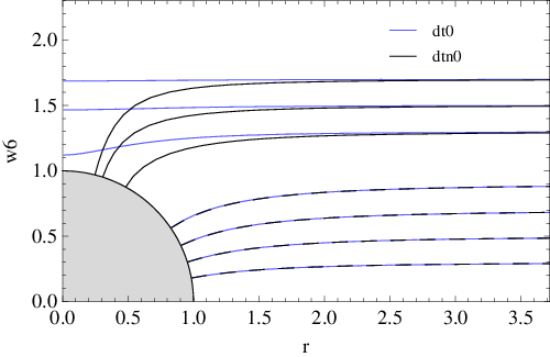
Examples for embeddings are shown in fig. 1. In the case of vanishing particle density we observe both black hole embeddings, ending on the black hole horizon, and Minkowski embeddings [23]. The latter embeddings do not touch the horizon. For any finite value of the particle density there are only black hole embeddings [27].

Figure 1: Embedding function $L(r)$ of D$7$-branes in the AdS black hole background, with the dimensionless coordinates $L=\rho\cos\theta=\rho\chi$ and $r=\rho\sin\theta=\rho\sqrt{1-\chi^{2}}$.

2.3.4 Strings from branes

In the case of pure finite baryon density [27] it was shown that D$7$-branes representing heavy quarks develop a spike near the horizon, since they reach the horizon albeit their large value of $L$ at large $r$. This spike may be interpreted as a bundle of strings stretching between the D$7$-branes and the black hole. This bundle of strings is necessary in the presence of a non-vanishing gauge field on the brane. Since in our case we have a similar setup, we expect to have this spike, too. To formalize this intuition, we analyze the near horizon limit of the brane embedding in more detail as in [27]. We start by writing the Legendre-transformed action as

$$\tilde{S}_{\text{DBI}}=-\frac{T_{D7}}{\sqrt{2}}\int\!\mathrm{d}^{8}\xi\;\frac{f}{\sqrt{\tilde{f}}}\sqrt{1+\frac{\varrho^{2}(\partial_{\varrho}\chi)^{2}}{1-\chi^{2}}}\sum_{i=1}^{N_{f}}\sqrt{\frac{d_{i}^{2}}{(2\pi\alpha^{\prime})^{2}T_{D7}}+\frac{\varrho^{6}\tilde{f}^{3}(1-\chi^{2})^{3}}{8}}\,.$$ (2.46)

Notice that $\chi=\cos\theta$, which becomes $\chi\simeq 1$ if the embedding is very near to the axis. Therefore, the second term in the square roots can be neglected and we get

$$\tilde{S}_{\text{DBI}} =-\frac{V_{3}\text{vol}(S^{3})}{2\pi\alpha^{\prime}}\left(\sum_{i=1}^{N_{f}}d_{i}\right)\int\!\mathrm{d}t\mathrm{d}\varrho\;\frac{f}{\sqrt{2\tilde{f}}}\sqrt{1+\frac{\varrho^{2}(\partial_{\varrho}\chi)^{2}}{1-\chi^{2}}}$$

$$=-\frac{V_{3}\text{vol}(S^{3})}{2\pi\alpha^{\prime}}\left(\sum_{i=1}^{N_{f}}d_{i}\right)\int\!\mathrm{d}t\mathrm{d}\varrho\;\sqrt{-g_{tt}(g_{\varrho\varrho}+g_{\theta\theta}(\partial_{\varrho}\theta)^{2})}\,,$$ (2.47)

where $V_{3}$ is the Minkowski space volume and $\text{vol}(S^{3})$ the volume of the 3-sphere. Recognize the fact that the result above can be written as the Nambu-Goto action for a bundle of strings stretching in $\varrho$ direction but free bending in the $\theta$ direction,

$$\tilde{S}_{\text{DBI}}=-V_{3}\text{vol}(S^{3})\left(\sum_{i=1}^{N_{f}}d_{i}\right)S_{NG}\,.$$ (2.48)

Therefore just one of the densities $d_{i}$ must be non-zero to make the branes develop a spike close to the axis. This is the expected result. According to the discussion below equation (2.13) we consider a consistent case in which the $N_{f}$ branes are coincident. Therefore they have the same embedding function, such that the complete stack of $N_{f}$ D$7$-branes develops the spike discussed above.

2.4 Numerical results for the background fields
at constant baryon and isospin density

Figure 2: The dimensionless mass parameter $m$ as defined in equation (2.45) versus the horizon value $\chi_{0}=\lim_{\rho\to 1}\chi$ of the embedding at baryon density $\tilde{d}^{B}=0.5$ for the case $N_{f}=2$. The five different curves correspond to isospin density $\tilde{d}^{I}=0$ (black), $\tilde{d}^{I}=\frac{1}{4}\tilde{d}^{B}$ (green), $\tilde{d}^{I}=\frac{1}{2}\tilde{d}^{B}$ (blue), $\tilde{d}^{I}=\frac{3}{4}\tilde{d}^{B}$ (red) and $\tilde{d}^{I}=\tilde{d}^{B}$ (orange).

Figure 3: The dimensionless chiral condensate $c$ versus the mass parameter $m$ as defined in equation (2.45) at baryon density $\tilde{d}^{B}=5\cdot 10^{-5}$ (a), $\tilde{d}^{B}=0.5$ (b) and $\tilde{d}^{B}=20$ (c) for the case $N_{f}=2$. The five different curves in each figure correspond to isospin density $\tilde{d}^{I}=0$ (black), $\tilde{d}^{I}=\frac{1}{4}\tilde{d}^{B}$ (green), $\tilde{d}^{I}=\frac{1}{2}\tilde{d}^{B}$ (blue), $\tilde{d}^{I}=\frac{3}{4}\tilde{d}^{B}$ (red) and $\tilde{d}^{I}=\tilde{d}^{B}$ (orange).

Figure 4: The baryon (left) and isospin (right) chemical potential divided by the bare quark mass $M_{q}$ versus the mass parameter $m$ as defined in equation (2.45) at baron density $\tilde{d}^{B}=5\cdot 10^{-5}$ in the upper figures and $\tilde{d}^{B}=0.5$ in the lower ones for the case $N_{f}=2$. The five different curves in each figure correspond to isospin density $\tilde{d}^{I}=0$ (black), $\tilde{d}^{I}=\frac{1}{4}\tilde{d}^{B}$ (green), $\tilde{d}^{I}=\frac{1}{2}\tilde{d}^{B}$ (blue), $\tilde{d}^{I}=\frac{3}{4}\tilde{d}^{B}$ (red) and $\tilde{d}^{I}=\tilde{d}^{B}$ (orange).

In this section we present numerical results for the background fields at constant densities, which will later be used to determine the thermodynamics in the canonical ensemble. We first analyze the embedding of the D$7$-branes. Fig. 2 and 3 show the dependence of the mass parameter $m$ on the horizon value of the embedding function $\chi_{0}=\lim_{\rho\to 1}\chi$ and of the chiral condensate $c$ on the mass parameter $m$ for the case $N_{f}=2$ at different baryon and isospin densities.

Fig. 2 shows the same divergent behavior of the mass parameter as found in [27] for the pure baryonic case. Fig. 3 (a) shows that the low temperature black hole embeddings for small but non-zero densities mimic the behavior of Minkowski embeddings which describe the brane at zero densities. For small densities there is a first order phase transition between two black hole embeddings, which replaces the first order phase transition between black hole and Minkowski embeddings at zero densities [23, 25]. Later in section 3.2 we discuss that the phase transition between the two black hole embeddings must be replaced by a phase transition between black hole embeddings and an inhomogeneous mixture of black hole and Minkowski embeddings since the black hole embeddings alone are not the stable ground state of this theory. At a baryon density larger than a critical density, which value depends on the isospin density, the phase transition disappears and a local maximum appears in the chiral condensate (see fig. 3 (b)). This maximum disappears if we increase the baryon or the isospin density and the chiral condensate $c$ monotonically decreases as we increase the mass $m$ (see fig 3 (c)).

Fig. 3 also shows that for finite densities, the chiral condensate $c$ approaches a fixed non-zero value in the limit $m\to\infty$, i. e. $T\to 0$. In fig. 3 (a) this asymptotic value is small due to the small baryon density but also non-zero as in fig. 3 (b) and (c). Since the non-zero chiral condensate breaks conformal invariance and supersymmetry, these symmetries are always broken in our setup even in the limit $T\to 0$, where the AdS black hole background becomes conformal and supersymmetric. This symmetry breaking is induced by the finite densities and chemical potentials. The finite densities, which introduce a new scale, break conformal invariance. The non-zero vev of just the time component of the gauge field, which describes the chemical potential, breaks Lorentz invariance and therefore supersymmetry.

Next we present the chemical potentials $\mu^{B}$ and $\mu^{I}$ in fig. 4 for the case $N_{f}=2$ at different baryon and isospin densities. In the limit $m\to\infty$, the baryon chemical potential $\mu^{B}$ approaches $M_{q}$ and the isospin chemical potential $\mu^{I}$ approaches 0 (see fig. 4 black, green, blue and red line) for $\tilde{d}^{B}>\tilde{d}^{I}\geq 0$ as shown in equation (2.41). For $\tilde{d}^{B}=\tilde{d}^{I}$ (orange line) the baryon and isospin chemical potential both approach $M_{q}/2$ in the large mass limit as shown in equation (2.42). Moreover, fig. 4 (c) and (d) show that the baryon chemical potential is independent of the isospin density except for the discontinuous step at $\tilde{d}^{B}=\tilde{d}^{I}$ and the isospin chemical potential obviously depends on the isospin density. Fig. 4 (a) and (b) show that the phase transition is also visible in the chemical potential. For a baryon density smaller than the critical density, the dimensionless quantities $\mu^{B/I}/M_{q}$ decrease as we decrease the mass $m$ and stays constant at a non-vanishing but small value after the phase transition. For a baryon density larger than the critical density, the dimensionless quantities $\mu^{B/I}/M_{q}$ diverge in the small mass limit $m\to 0$.

2.5 Numerical results for the background fields
at constant baryon and isospin chemical potential

In the calculations above we treated the densities $\tilde{d}^{B}$ and $\tilde{d}^{I_{i}}$ as a independent variables since they are the constants of motion. Thermodynamically this means that we consider the canonical ensemble. Since we also would like to study the grand canonical ensemble with the chemical potentials $\tilde{\mu}^{B}$ and $\tilde{\mu}^{I_{i}}$ as independent variables, we must analyze the background fields for constant chemical potentials $\tilde{\mu}^{B}$ and $\tilde{\mu}^{I_{i}}$. To determine the densities $\tilde{d}_{i}$ for a given chemical potential $\tilde{\mu}_{i}$ we must invert equation (2.37). We use a shooting method to obtain these functions $\tilde{d}_{i}(\tilde{\mu}_{i},m)$.

So far we considered only the case with non-zero densities. We now investigate the case with zero densities but still non-zero chemical potentials. As shown in [51], in this case Minkowski embeddings must also be included. Since the action only depends on the derivative of the gauge field, a Minkowski embedding with constant gauge field solves the equation of motion. Therefore, on these Minkowski embeddings the chemical potential can take any value. The equation of motion for the Minkowski embedding $L$ is given by [25]

$$\partial_{r}\left[r^{3}\left(1-\frac{1}{(r^{2}+L^{2})^{4}}\right)\frac{\partial_{r}L}{\sqrt{1+(\partial_{r}L)^{2}}}\right]-8\frac{r^{3}L}{(r^{2}+L^{2})^{5}}\sqrt{1+(\partial_{r}L)^{2}}=0\,,$$ (2.49)

where $L$ and $r$ are dimensionless and given by $\rho^{2}=r^{2}+L^{2}$, $r=\rho\sin\theta=\rho\sqrt{1-\chi^{2}}$ and $L=\rho\cos\theta=\rho\chi$. From now on we only use these dimensionless coordinates $L$ and $r$. The asymptotic solution for the embedding function $L$ close to the boundary is,

$$L=m+\frac{c}{r^{2}}+\cdots\,.$$ (2.50)

The parameters $m$ and $c$ are related to the quark mass $M_{q}$ and the chiral condensate $\langle\bar{\psi}\psi\rangle$ given by equation (2.45). Using the initial conditions $L(r=0)=L_{0}$ and $\partial_{r}L(r=0)=0$, we may solve the equation of motion (2.49) numerically. The parameters $m$ and $c$ may be determined by fitting the numerical solutions to the asymptotic form (2.50).

In fig. 5, 6, 7 and 8 we show numerical results for the background fields at constant chemical potential. Fig. 5 shows the mass parameter $m$ versus the horizon value of the black hole embeddings $\chi_{0}$ between 0 and 1 and the asymptotic value of the Minkowski embeddings $L_{0}$ between 1 and 2 at different baryon and isospin chemical potentials. In these figures we see that there is a region where the Minkowski and the black hole embeddings generate the same mass parameter $m$. We will show in section 4.2 that in this overlap there is a first order phase transition as in the case of zero chemical potential [23, 25]. For small chemical potentials (see fig. 5 (a)), the mass parameter decreases in the black hole phase for $\chi_{0}\to 1$ as known from [23, 25]. However, for larger chemical potentials (see fig. 5 (b)), the mass parameter $m$ increases monotonically as we increase $\chi_{0}$. In both cases, fig. 5 (a) and (b) demonstrate that the mass parameter depends linearly on the the asymptotic values $\chi_{0}$ and $L_{0}$ in a large region. The only non-linear behavior is in the region where both embeddings can be constructed. For chemical potentials $(\mu^{B}+\mu^{I})/M_{q}>1$ (fig. 5 (c)), the mass parameter diverges as $\chi_{0}\to 1$ as in the case of constant densities. This corresponds to the fact that in the canonical ensemble, there are black hole embeddings for all mass parameters $m$. In the grand canonical ensemble, however, there are also Minkowski embeddings.

Figure 5: The dimensionless mass parameter $m$ as defined in equation (2.45) versus the horizon value of the black hole embeddings $\chi_{0}=\lim_{\rho\to 1}\chi$ between 0 to 1 and the asymptotic value of the Minkowski embeddings $L_{0}=\lim_{r\to 0}L$ between 1 and 2 at baryon chemical potential $\mu^{B}/M_{q}=0.01$ (a), $\mu^{B}/M_{q}=0.1$ (b) and $\mu^{B}/M_{q}=0.8$ (c) for the case $N_{f}=2$. The dotted purple curve corresponds to Minkowski embeddings and the five other curves to black hole embeddings with isospin chemical potential $\mu^{I}=0$ (black), $\mu^{I}=\frac{1}{4}\mu^{B}$ (green), $\mu^{I}=\frac{1}{2}\mu^{B}$ (blue), $\mu^{I}=\frac{3}{4}\mu^{B}$ (red) and $\mu^{I}=\mu^{B}$ (orange).

Figure 6: The dimensionless chiral condensate $c$ versus the mass parameter $m$ as defined in equation (2.45) at baryon chemical potential $\mu^{B}/M_{q}=0.01$ (a), $\mu^{B}/M_{q}=0.1$ (b) and $\mu^{B}/M_{q}=0.8$ (c) for the case $N_{f}=2$. The dotted purple curve corresponds to Minkowski embeddings and the five other curves to black hole embeddings with isospin chemical potential $\mu^{I}=0$ (black), $\mu^{I}=\frac{1}{4}\mu^{B}$ (green), $\mu^{I}=\frac{1}{2}\mu^{B}$ (blue), $\mu^{I}=\frac{3}{4}\mu^{B}$ (red) and $\mu^{I}=\mu^{B}$ (orange).

Figure 7: The dimensionless baryon density $\tilde{d}^{B}$ versus the mass parameter $m$ as defined in equation (2.45) at baryon chemical potential $\mu^{B}/M_{q}=0.01$ (a), $\mu^{B}/M_{q}=0.1$ (b) and $\mu^{B}/M_{q}=0.8$ (c) for the case $N_{f}=2$. The five different curves correspond to black hole embeddings with isospin chemical potential $\mu^{I}=0$ (black), $\mu^{I}=\frac{1}{4}\mu^{B}$ (green), $\mu^{I}=\frac{1}{2}\mu^{B}$ (blue), $\mu^{I}=\frac{3}{4}\mu^{B}$ (red) and $\mu^{I}=\mu^{B}$ (orange). In the Minkowski phase, the baryon density is always zero and is therefore not shown in the figures.

Figure 8: The dimensionless isospin density $\tilde{d}^{I}$ versus the mass parameter $m$ as defined in equation (2.45) at baryon chemical potential $\mu^{B}/M_{q}=0.01$ (a), $\mu^{B}/M_{q}=0.1$ (b) and $\mu^{B}/M_{q}=0.8$ (c) for the case $N_{f}=2$. The five different curves correspond to black hole embeddings with isospin chemical potential $\mu^{I}=0$ (black), $\mu^{I}=\frac{1}{4}\mu^{B}$ (green), $\mu^{I}=\frac{1}{2}\mu^{B}$ (blue), $\mu^{I}=\frac{3}{4}\mu^{B}$ (red) and $\mu^{I}=\mu^{B}$ (orange). In the Minkowski phase, the isospin density is always zero and is therefore not shown in the figures. For a zero isospin chemical potential $\mu^{I}=0$, the isospin density $\tilde{d}^{I}$ is also zero and therefore coincides with the $m$-axis.

Fig. 6 shows the chiral condensate $c$ versus the mass parameter $m$ at different baryon and isospin chemical potentials. For small chemical potentials (fig. 6 (a) and (b)), we see a similar behavior as in the case of zero chemical potentials [23, 25]. By increasing the chemical potentials, the spiral behavior of the chiral condensate vanishes since the mass parameter increases monotonically as we increase $\chi_{0}$. However, there is still a region where the chiral condensate is multivalued since there are black hole and Minkowski embeddings which generate the same mass $m$. For large chemical potentials $(\mu^{B}+\mu^{I})/M_{q}>1$ (fig. 6 (c)), the chiral condensate diverges as we increase $m$. Since for smaller chemical potentials $(\mu^{B}+\mu^{I})/M_{q}<1$ the chiral condensate in the black hole phase approaches the value for Minkowski embeddings at a finite mass $m$, the divergent behavior of the chiral condensate for large chemical potentials $(\mu^{B}+\mu^{I})/M_{q}>1$ indicates that there is no phase transition between black hole and Minkowski embeddings anymore.

Fig. 7 and 8 show the baryon and isospin density versus the mass parameter $m$ calculated by the inversion of equation (2.37) at different baryon and isospin chemical potentials. These figures show that for all chemical potentials $\mu^{B/I}$, the baryon and the isospin density are zero at zero mass $m=0$. For small chemical potential, fig. 7 (a), (b) and 8 (a), (b) show that the densities increase until they reach a maximum at $m\sim 1$. Beyond the maximum the densities decreases rapidly, but they do not reach to zero at the largest $m$ which can be constructed by black hole embeddings. Therefore, there is also a discontinuous step in the densities as in the chiral condensate at the transition from black hole embeddings to Minkowski embeddings. For large chemical potentials $(\mu^{B}+\mu^{I})/M_{q}>1$ (fig. 7 (c) and 8 (c)), the densities diverge as we increase $m$, as does the chiral condensate.

3 Canonical D$7$-brane thermodynamics

3.1 The canonical ensemble:
free energy, entropy, energy and speed of sound

In this section we study the thermodynamic behavior of the quark sector at finite baryon and isospin density which is dual to thermal contributions of the D$7$-branes. Since the partition function $Z$ of the field theory is given according the AdS/CFT dictionary by

$$Z={\mathrm{e}}^{-S_{\text{on-shell}}}\,,$$ (3.1)

with the Euclidean on-shell supergravity action $S_{\text{on-shell}}$, the thermodynamical potential, in the canonical ensemble the free energy $F$, is proportional to the Euclidean on-shell action

$$F=-T\ln Z=TS_{\text{on-shell}}\,.$$ (3.2)

To calculate the thermal contributions of the D$7$-branes $F_{7}$, we have to determine the Euclidean DBI action (2.23) on-shell.

First we perform a Wick rotation in the time direction to obtain the Euclidean DBI-action. Next we must renormalize this action by adding the appropriate counterterms $I_{\text{ct}}$ (see [52] for a review) since it diverges on-shell. Since these counterterms do not depend on the finite densities, we can write them as in [25, 27],

$$I_{\text{ct}}=-\frac{{\cal N}_{\lambda}}{4}\left[\left(\rho_{\text{max}}^{2}-m^{2}\right)^{2}-4mc\right]\,,$$ (3.3)

where $\rho_{\text{max}}$ is the UV-cutoff and

$${\cal N}_{\lambda}=\frac{T_{D7}V_{3}\text{vol}(S^{3})N_{f}\varrho_{H}^{4}}{4T}=\frac{\lambda N_{c}N_{f}V_{3}T^{3}}{32}\,,$$ (3.4)

whit the Minkowski space volume $V_{3}$. Then the renormalized Euclidean on-shell action $I_{R}$ may simply be written as

$$\frac{I_{R}}{{\cal N}_{\lambda}}=\frac{1}{N_{f}}G(m,\tilde{\mu})-\frac{1}{4}\left[\left(\rho_{\text{min}}^{2}-m^{2}\right)^{2}-4mc\right]\,,$$ (3.5)

where $\rho_{\text{min}}$ determines the minimal value of the coordinate $\rho$ on the D$7$-branes, i. e. $\rho_{\text{min}}=1$ for black hole embeddings and $\rho_{\text{min}}=L_{0}$ for Minkowski embeddings and

$$\begin{split}G(m,\tilde{\mu})=\int_{\rho_{\text{min}}}^{\infty}\!\mathrm{d}\rho\;\Bigg(&\rho^{3}f\tilde{f}\left(1-\chi^{2}\right)\\ &\times\sum_{i=1}^{N_{f}}\sqrt{1-\chi^{2}+\rho^{2}(\partial_{\rho}\chi)^{2}-2\frac{\tilde{f}}{f^{2}}(1-\chi^{2})(\partial_{\rho}\tilde{X}_{i})^{2}}\\ &-N_{f}\left(\rho^{3}-\rho m^{2}\right)\Bigg)\,.\end{split}$$ (3.6)

Since this action depends on the background fields $\chi$ and $X_{i}$ and therefore on the mass parameter $m$ and the chemical potential $\mu_{i}$, it is proportional to the grand potential in the grand canonical ensemble. To get the free energy in the canonical ensemble, we must perform a Legendre transformation of the on-shell action $I_{R}$ as we did in equation (2.27). The Legendre transformed on-shell action $\tilde{I}_{R}$ is given by

$$\frac{\tilde{I}_{R}}{{\cal N}_{\lambda}}=\frac{1}{N_{f}}\tilde{G}(m,\tilde{d})-\frac{1}{4}\left[\left(\rho_{\text{min}}^{2}-m^{2}\right)^{2}-4mc\right]\,,$$ (3.7)

where

$$\begin{split}\tilde{G}(m,\tilde{d})=\int_{\rho_{\text{min}}}^{\infty}\!\mathrm{d}\rho\;\Bigg(&\rho^{3}f\tilde{f}\left(1-\chi^{2}\right)\sqrt{1-\chi^{2}+\rho^{2}(\partial_{\rho}\chi)^{2}}\\ &\times\sum_{i=1}^{N_{f}}\sqrt{1+\frac{8\tilde{d}_{i}^{2}}{\rho^{6}\tilde{f}^{3}(1-\chi^{2})^{3}}}-N_{f}\left(\rho^{3}-\rho m^{2}\right)\Bigg)\,.\end{split}$$ (3.8)

In the following we use this action to calculate the main thermodynamical quantities. The difference to the results obtained in [27] is induced by the sum over the $N_{f}$ different densities in equation (3.8).

3.1.1 The free energy

The contribution of the D$7$-branes to the Helmholtz free energy is

$$F_{7}=T\tilde{I}_{R}=\frac{\lambda N_{c}N_{f}V_{3}T^{4}}{32}{\cal F}_{7}(m,\tilde{d})$$ (3.9)

with the dimensionless quantity

$${\cal F}_{7}(m,\tilde{d})=\frac{\tilde{I}_{R}}{{\cal N}_{\lambda}}=\frac{1}{N_{f}}\tilde{G}(m,\tilde{d})-\frac{1}{4}\{(\rho_{\text{min}}^{2}-m^{2})^{2}-4mc\}\,.$$ (3.10)

The dimensionless quantity ${\cal F}_{7}$ determines the dependence of the free energy $F$ of the complete setup on the quark mass $M_{q}$ and the quark densities $n_{q}$ at a fixed temperature $T$.

Using the example of the free energy we study how a thermodynamic quantity of the complete setup is composed of the quantities of the subsystems. The parts from the D3-branes $F_{3}$, which is the known quantity for the conformal ${\cal N}=4$ SYM theory, and from D$7$-branes $F_{7}$ form the free energy of the complete setup

$$\begin{split}F&=F_{3}+F_{7}=-\frac{\pi^{2}}{8}N_{c}^{2}V_{3}T^{4}+\frac{\lambda N_{c}N_{f}V_{3}T^{4}}{32}{\cal F}_{7}(m,\tilde{d})\\ &=-\frac{\pi^{2}}{8}N_{c}^{2}V_{3}T^{4}\left(1-\frac{\lambda N_{f}}{4\pi^{2}N_{c}}{\cal F}_{7}(m,\tilde{d})\right)\,.\end{split}$$ (3.11)

Here we only get the first order contribution in $N_{f}/N_{c}$ since we work in the probe brane limit $N_{f}\ll N_{c}$. In the following we define quantities similar to ${\cal F}_{7}$ for the other thermodynamic quantities and denote them also with a calligraphic letter. Note that these thermal contributions of the D$7$-branes vanish in the limit where supersymmetry and conformal invariance is restored. This limit is given by zero densities and large mass parameters $m\to\infty$.

3.1.2 The entropy

As in [25, 27], the contribution to the entropy by the D$7$-branes is given by

$$S_{7}=-\frac{\partial F_{7}}{\partial T}=-\pi R^{2}\frac{\partial F_{7}}{\partial\varrho_{H}}=\frac{\lambda N_{c}N_{f}V_{3}T^{3}}{32}{\cal S}_{7}(m,\tilde{d})\,,$$ (3.12)

with the mass and density dependent part

$${\cal S}_{7}(m,\tilde{d})=-4{\cal F}_{7}(m,\tilde{d})+\frac{12}{N_{f}}\sum_{i=1}^{N_{f}}\tilde{d}_{i}\tilde{\mu}_{i}-2mc\,.$$ (3.13)

In comparison to the case without isospin density [27], there is sum over the $N_{f}$ different densities.

3.1.3 The energy

Using the thermodynamic relation $E=F+TS$, we calculate the energy

$$E_{7}=\frac{\lambda N_{c}N_{f}V_{3}T^{4}}{32}{\cal E}_{7}(m,\tilde{d})\,,$$ (3.14)

with the dimensionless quantity

$${\cal E}_{7}(m,\tilde{d})=-3{\cal F}_{7}(m,\tilde{d})+\frac{12}{N_{f}}\sum_{i=1}^{N_{f}}\tilde{d}_{i}\tilde{\mu}_{i}-2mc\,.$$ (3.15)

Again a sum over the $N_{f}$ densities appears in the equation above, which is due to the finite isospin densities.

3.1.4 The speed of sound

The speed of sound is given by

$$v_{s}^{2}=\frac{V_{3}\partial P}{\partial E}=-\frac{\partial(\Omega_{3}+\Omega_{7})}{\partial T}\cdot\frac{\partial T}{\partial(E_{3}+E_{7})}\,,$$ (3.16)

where the pressure $P$ is given by $PV_{3}=-\Omega=-(\Omega_{3}+\Omega_{7})$. $\Omega$ and $E$ are the grand potential and energy of the complete system. $\Omega_{3}$ and $E_{3}$ are the contribution to the grand potential and energy of the D3-branes, respectively. Using the thermodynamic relations $S=-\left(\frac{\partial F}{\partial T}\right)_{V,N}=-\left(\frac{\partial\Omega}{\partial T}\right)_{V,\mu}$ and $c_{v}=\left(\frac{\partial E}{\partial T}\right)_{V,N}$, we may rewrite the speed of sound in the canonical ensemble

$$v_{s}^{2}=\frac{S_{3}+S_{7}}{c_{v3}+c_{v7}}\,.$$ (3.17)

Using equation (3.15) the specific heat $c_{v7}$ becomes

$$c_{v7}=3S_{7}-\frac{3\lambda N_{c}N_{f}V_{3}T^{3}}{16}\left(mc-\frac{1}{3}m^{2}\frac{\partial c}{\partial m}+\frac{2}{N_{f}}\sum_{i=1}^{N_{f}}\tilde{d}_{i}\left(m\frac{\partial\tilde{\mu}_{i}}{\partial m}-4\tilde{\mu}_{i}\right)\right)\,,$$ (3.18)

where we used $\partial_{T}=-\frac{m}{T}\partial_{m}$ (see equation (2.45)). With the contributions of the D$3$-branes given by the thermodynamics of the conformal ${\cal N}=4$ SYM theory,

$$S_{3}=\frac{\pi^{2}}{2}V_{3}N_{c}^{2}T^{3}\qquad\text{and}\qquad c_{v3}=3S_{3}\,,$$ (3.19)

we evaluate the speed of sound to first order in $N_{f}/N_{c}$

$$v_{s}^{2}=\frac{1}{3}\left[1+\frac{\lambda N_{f}}{8\pi^{2}N_{c}}{\cal V}_{s}^{2}(m,\tilde{d})\right]\,,$$ (3.20)

with

$${\cal V}_{s}^{2}(m,\tilde{d})=mc-\frac{1}{3}m^{2}\frac{\partial c}{\partial m}+\frac{2}{N_{f}}\sum_{i=1}^{N_{f}}\tilde{d}_{i}\left(m\frac{\partial\tilde{\mu}_{i}}{\partial m}-4\tilde{\mu}_{i}\right)\,.$$ (3.21)

Notice that the first order correction in $N_{f}/N_{c}$ is consistent with the approximation of probe branes (cf. with equation (3.11)). The last term reflects the presence of the finite baryon and isospin density. The dependence on the mass parameter $m$ and the chiral condensate $c$ is given by the result without densities [25].

3.1.5 Numerical results for the free energy, entropy, energy and the speed of sound

Figure 9: The dimensionless free energy ${\cal F}_{7}$ versus the mass parameter $m$ as defined in equation (2.45) at baryon density $\tilde{d}^{B}=5\cdot 10^{-5}$ (left) and $\tilde{d}^{B}=2$ (right) for the case $N_{f}=2$. The five different curves in each figure correspond to $\tilde{d}^{I}=0$ (black), $\tilde{d}^{I}=\frac{1}{4}\tilde{d}^{B}$ (green), $\tilde{d}^{I}=\frac{1}{2}\tilde{d}^{B}$ (blue), $\tilde{d}^{I}=\frac{3}{4}\tilde{d}^{B}$ (red) and $\tilde{d}^{I}=\tilde{d}^{B}$ (orange).

Figure 10: The dimensionless entropy ${\cal S}_{7}$ versus the mass parameter $m$ as defined in equation (2.45) at baryon density $\tilde{d}^{B}=0.5$ (left) and $\tilde{d}^{B}=2$ (right) for the case $N_{f}=2$. The five different curves in each figure correspond to $\tilde{d}^{I}=0$ (black), $\tilde{d}^{I}=\frac{1}{4}\tilde{d}^{B}$ (green), $\tilde{d}^{I}=\frac{1}{2}\tilde{d}^{B}$ (blue), $\tilde{d}^{I}=\frac{3}{4}\tilde{d}^{B}$ (red) and $\tilde{d}^{I}=\tilde{d}^{B}$ (orange).

Figure 11: The dimensionless energy ${\cal E}_{7}$ versus the mass parameter $m$ as defined in equation (2.45) at baryon density $\tilde{d}^{B}=0.5$ (left) and $\tilde{d}^{B}=2$ (right) for the case $N_{f}=2$. The five different curves in each figure correspond to $\tilde{d}^{I}=0$ (black), $\tilde{d}^{I}=\frac{1}{4}\tilde{d}^{B}$ (green), $\tilde{d}^{I}=\frac{1}{2}\tilde{d}^{B}$ (blue), $\tilde{d}^{I}=\frac{3}{4}\tilde{d}^{B}$ (red) and $\tilde{d}^{I}=\tilde{d}^{B}$ (orange).

Figure 12: The dimensionless speed of sound relative to the conformal case ${\cal V}_{s}^{2}$ versus the mass parameter $m$ as defined in equation (2.45) at baryon density $\tilde{d}^{B}=5\cdot 10^{-5}$ (a), $\tilde{d}^{B}=0.5$ (b) and $\tilde{d}^{B}=2$ (c) for the case $N_{f}=2$. The five different curves in each figure correspond to $\tilde{d}^{I}=0$ (black), $\tilde{d}^{I}=\frac{1}{4}\tilde{d}^{B}$ (green), $\tilde{d}^{I}=\frac{1}{2}\tilde{d}^{B}$ (blue), $\tilde{d}^{I}=\frac{3}{4}\tilde{d}^{B}$ (red) and $\tilde{d}^{I}=\tilde{d}^{B}$ (orange).

In fig. 9, 10, 11 and 12 we present numerical results for the mass and density dependent part of the thermodynamic quantities at different baryon and isospin densities for $N_{f}=2$.

Fig. 9 shows the free energy ${\cal F}_{7}$ versus the mass parameter $m$ at different densities as calculated from equation (3.10). For small densities (see fig. 9 (a)) we see again that the low temperature black hole embeddings have the same free energy as the zero-density Minkowski embeddings. Since the free energy determines the thermodynamics entirely, the same effect is also seen in the other thermodynamic quantities and we therefore do not consider them at small densities. For larger densities (see fig. 9 (b)) we see a displacement due to the isospin densities, which is constant over a wide range. Moreover, the free energy behaves linearly for $m\gtrsim 2$. The increase of the free energy as $m\to\infty$ demonstrates the deviation from the conformal ${\cal N}=4$ thermodynamics which was discussed below equation (3.11). For small $m$, i. e. small quark masses compared to the temperature $M_{q}\ll T$, we see deviations from the linear behavior due to thermal fluctuations which increase the free energy.

In fig. 10 the entropy ${\cal S}_{7}$ versus the mass parameter $m$ as calculated from equation (3.13) is shown. Again a displacement due to the isospin densities appear. However, the displacement in the entropy becomes smaller as we increase $m$ and the entropy approaches a non-zero value independent of the isospin density as $m\to\infty$. Moreover if the baryon density is above its critical value, a minimum in the entropy appears for zero isospin density. By increasing the isospin density this minimum disappears slowly.

The energy ${\cal E}_{7}$ shown in fig. 11 as calculated from equation (3.15) shows a very similar behavior as the free energy, discussed above. However, a minimum appears in the energy at $m\approx 1.3$ for a baryon density above the critical density (see fig. 11 (a)). Increasing the baryon densities (see fig. 11 (b)), this minimum disappears.

Fig. 12 shows the speed of sound ${\cal V}_{s}^{2}$ calculated from equation (3.21). Again a displacement due to the isospin densities appear. In the speed of sound this displacement grow as we increase $m$. For a baryon density above the critical density and zero isospin density, the speed of sound is constant at $m\approx 1.3$ as shown in fig. 12 (b). Increasing the baryon or isospin density the speed of sound monotonously decreases as $m$ increases (fig. 12 (b) and (c)).

3.1.6 Interpretation: Quark mass selection and temperature change

Here we discuss the effect of a non-zero isospin density on the quark mass $M_{q}$. We argue that under certain conditions explained below, the thermodynamic quantities given in the previous section 3.1.5 select preferred values $M_{q}^{*}$ for the mass $M_{q}$ of the quarks inside the quark gluon plasma. In a slightly different setup we find that our system prefers a distinct temperature $T=T^{*}$.

In our model the quark mass $M_{q}$ is a free parameter. We fix the temperature $T$ and charge densities $n^{i}$ and keep the volume $V$ of our system constant. The canonical ensemble describes this situation with the free energy being the relevant thermodynamic potential. We argue how the quark mass $M_{q}$ as a free parameter has to be selected in order to satisfy the second law of thermodynamics. In fact we will find a competing behavior between entropy and energy requirements. The second law of thermodynamics implies that in thermal equilibrium, the entropy is maximized at fixed thermodynamic potential. This is equivalent to minimzing the thermodynamic potential at a fixed entropy [53]. In our case this potential is the free energy. However, competing situations between entropy and energy requirements are well known from frustrated systems, e. g. polymers or anti-ferromagnets on a triangle lattice, as well as glass states, e. g. spin glass [54]. In these systems the temperature is usually the thermodynamic variable which adjusts at a distinct value where the criteria are optimally satisfied. In our setup we have the quark mass $M_{q}$ as a free parameter, which in analogy to the case discussed above adjusts at a specific value $M_{q}^{*}$. In order to find this optimal value $M_{q}^{*}$, we examine figures 9 and 10. Recall from equations (2.45) and (2.35) that the mass parameter $m$ is related to the temperature and quark mass by $m=2M_{q}/(\sqrt{\lambda}T)$ and $n^{i}\propto\tilde{d}^{i}$. We observe that in the region $m\gtrsim 4$ for all densities, the free energy decreases at a constant entropy as the quark mass $M_{q}$ is increased. At smaller values of the mass parameter $m\lesssim 4$, the entropy changes as we vary the quark mass $M_{q}$. The second law of thermodynamics forbids the system to be in equilibrium. From these considerations and from looking at figures 9 and 10 we conclude that the quark mass has to take a value of $0\leq M_{q}^{*}\leq\sqrt{\lambda}Tm/2$, such that $0\leq m\leq 4$. Since in this regime the entropy and free energy both vary when the densities are changed, we expect the value of $M_{q}$ to depend on the densities $n^{i}$, i.e. $M_{q}=M_{q}^{*}(n^{i})$. Therefore, our system with the quark mass as a free parameter shows similar properties as the frustrated systems discussed above.

It is amusing to apply the results of this analysis to the quark gluon plasma formed after the big bang. This would imply that our universe could have evolved in such a way that the quark mass was chosen such that it optimizes the free energy and entropy requirements. Note that during this mass selection process we have to stay in a regime where the metric does not change considerably in order for this system to be approximately closed [53].

Now we consider a different scenario, by which a distinct temperature $T^{*}$ is favored. We work in the microcanonic ensemble by fixing the entropy instead of temperature. An example of such a situation is the collision of heavy ions in vacuum. Since the natural temperature variable for our system is the temperature $T$ measured in units of the quark mass $M_{q}$, we let $m$ change freely. In this case the quark mass $M_{q}$ is fixed and the volume of plasma evolves to a preferred value of temperature $T$, in a reversible thermodynamic process. The system seeks to minimize its internal energy ${\cal E}_{7}$ while its entropy ${\cal S}_{7}$ is fixed by definition. In this setup the plasma relaxes isentropically to a favored temperature $T=T^{*}$.

3.2 Phase transition/phase diagram in the canonical ensemble

Figure 13: (a) The dimensionless free energy ${\cal F}_{7}$, (b) the speed of sound ${\cal V}_{s}^{2}$, (c) the chiral condensate $c$, (d) the baryon chemical potential $\mu^{B}/M_{q}$ and (e) the isospin chemical potential $\mu^{I}/M_{q}$ versus the mass parameter $m$ as defined in equation (2.45) near the phase transition at the baryon density $\tilde{d}^{B}=5\cdot 10^{-5}$ for $N_{f}=2$. The resolution of the figures is not high enough to dissolve the curves at different isospin density $\tilde{d}^{I}=0,\frac{1}{4}\tilde{d}^{B},\frac{1}{2}\tilde{d}^{B},\frac{3}{4}\tilde{d}^{B},\tilde{d}^{B}$. The dashed line at $m=1.306$ marks the phase transition.

Figure 14: (a) The phase diagram in the canonical ensemble for $N_{f}=2$: The cusp marks the phase transition for $\tilde{d}^{B}=\tilde{d}^{I}=0$ and the upper rim the critical points. Notice that the phase diagram is approximately $O(2)$ invariant in agreement with the symmetries discussed in section 2.3.1. (b) Position of the critical points: Comparison of the position of the critical points (cross) with the $O(2)$ invariant circle (blue) and a superellipse $(\tilde{d}^{I})^{a}=(\tilde{d}^{B}_{\text{crit}})^{a}-(\tilde{d}^{B})^{a}$ with $a=2.08$ (dashed). The difference of the parameter a from 2 determines the deviation from the $O(2)$ symmetry.

In the pure baryonic case [27] it was shown that there is a first order phase transition between two black hole embeddings for densities below the critical density $\tilde{d}^{B}_{\text{crit}}=0.0063$. In this section we analyze how the isospin density influences this phase transition. In fig. 13 we give an example of the behavior of the free energy, the speed of sound, the chiral condensate, the baryon and the isospin chemical potential $\mu^{B/I}/M_{q}$ close to the phase transition. The free energy, the speed of sound and the chiral condensate behave as in the pure baryonic case [27]. The isospin chemical potential $\mu^{I}/M_{q}$ takes different values depending on the isospin density after the phase transition (see fig. 13 (e)). The baryon chemical potential (fig. 13 (d)) instead is almost independent of the isospin density. However, the behavior of both chemical potentials changes dramatically if the baryon and isospin densities are equal in agreement with equation (2.42).

Fig. 13 shows that the phase transition is first order since the free energy is continuous and the speed of sound, the chiral condensate and the chemical potentials show a multivalued behavior and therefore a discontinuous step at the phase transition. The phase transition is marked by the crossing point in the free energy of the two branches coming in from small $m$ and large $m$ (see fig. 13 (a)).

In fig. 14 (a) we map out the phase diagram by varying the densities and determining the crossing point in the free energy. As outlined in section 2.3.1, the phase diagram is approximately $O(2)$ invariant. We find a line of critical points, which mark the critical mass parameter $m_{\text{crit}}$ and critical densities $\tilde{d}^{B}_{\text{crit}}$, $\tilde{d}^{I}_{\text{crit}}$. For densities around the critical points, we expect the largest deviation to the $O(2)$ symmetry in the phase diagram (see equation (2.30)). To get a quantitative description of this deviation, we plot the critical points and compare them to the $O(2)$ invariant circle and the superellipse $(\tilde{d}^{I})^{a}=(\tilde{d}^{B}_{\text{crit}})^{a}-(\tilde{d}^{B})^{a}$ with $a=2.08$ in fig. 14 (b). The deviation $a-2=0.08$ is still small at the critical points. Thus, the complete phase boundary in the canonical ensemble is $O(2)$ invariant in a good approximation.

More advanced thermodynamical investigations of the pure baryonic case [27, 28] show that there is a region were the black hole embeddings are not a stable ground state for this theory. The points where the phase transition between the two black hole embeddings occurs is at the boundary of this unstable region. In [28] the authors expect that in this region an inhomogeneous mixture of black hole and Minkowski embeddings is the stable ground state. Therefore the phase transition is not between two black hole embeddings, but between a black hole embedding and this inhomogeneous mixture. The existence of a mixed phase is typical for a first order phase transition and can e. g. be observed in boiling water. The water does not instantly turn into gas but forms droplets consisting of a mixture of water and water vapor.

3.3 Canonical thermodynamics in the large quark mass limit

In the large mass limit $m\to\infty$, i. e. $M_{q}\gg T$, the dimensionless thermodynamic quantities and the chiral condensate vanish if the baryon and isospin densities are zero because supersymmetry and conformal symmetry are restored and therefore the thermodynamics are given by the results of the stack of D3-branes dual to the conformal ${\cal N}=4$ SYM theory [25]. Introducing finite baryon and isospin densities break these symmetries even though the AdS black hole background becomes symmetric and we get deviations in the thermodynamic quantities from the conformal results (see e. g. fig. 9). In the following we investigate the dependence of these deviations on the densities $\tilde{d}^{I_{i}}$ further.

3.3.1 Numerical results

Figure 15: (a) The baryon chemical potential $\mu^{B}/M_{q}$, (b) the isospin chemical potential $\mu^{I}/M_{q}$, (c) the chiral condensate $c$ and (d) the free energy ${\cal F}_{7}$ versus the baryon and isospin density at $m=20$, where the mass parameter $m$ is defined in equation (2.45), in the case $N_{f}=2$. (c) and (d) are contour plots of the chiral condensate and the free energy, respectively.

Figure 16: The phase diagram for $m\to\infty$, i. e. $M_{q}\gg T$: The dashed lines marks the phase transitions where the chemical potentials develop a discontinuous gap. Notice that the dashed lines are the fixed points of the symmetries $\tilde{d}_{1}\leftrightarrow-\tilde{d}_{1}$, $\tilde{d}_{2}\leftrightarrow-\tilde{d}_{2}$.

First we discuss the numerical results for the thermodynamic quantities, the chemical potentials and the chiral condensate at a fixed mass $m=20$ in dependence of the baryon and isospin density for $N_{f}=2$, presented in fig. 15. We restrict our analysis to non-negative baryon and isospin densities $\tilde{d}^{B},\tilde{d}^{I}\geq 0$. The results may be continued into the other three quadrants by the accidental symmetries, discussed in section 2.3.1.The discontinuous step in the chemical potentials along the line $\tilde{d}^{I}=\tilde{d}^{B}\geq 0$ described in (2.41) and (2.42) are shown in fig. 15 (a) and (b). We can easily characterize this behavior in the large mass limit $m\to\infty$ by

$$\frac{\mu^{B}}{M_{q}}\to H(\tilde{d}^{B}-\tilde{d}^{I})\qquad\text{and}\qquad\frac{\mu^{I}}{M_{q}}\to H(\tilde{d}^{I}-\tilde{d}^{B})\,,$$ (3.22)

where $H$ is the Heaviside function. This discontinuity suggests that there is a first order phase transition between the two regions $0\leq\tilde{d}^{I}<\tilde{d}^{B}$ and $0\leq\tilde{d}^{B}<\tilde{d}^{I}$. At the same line the chiral condensate and the thermodynamic quantities develop a kink (see fig. 15), which also indicates that there is a phase boundary along the line $\tilde{d}^{B}=\tilde{d}^{I}\geq 0$. Using the accidental symmetries discussed in section 2.3.1, we give an overview of the four different phases and the values of the chemical potentials in the corresponding region in fig. 16. The same four different phases are also seen in QCD-like theories studied in [46]. Since in [46] the authors study the grand canonical ensemble, the phase transition is marked by a discontinuous step in the baryon and isospin density and phase boundaries are given by $|\mu^{B}|=|\mu^{I}|$. Along these phase boundaries the chiral condensate develops a similar kink as we observe here.

From the contour plot in fig. 15 (c), we see that the chiral condensate is independent of the isospin density for large masses in the region $0\leq\tilde{d}^{I}<\tilde{d}^{B}$ since the contour lines are parallel to the lines of constant baryon density in the region $0\leq\tilde{d}^{I}<\tilde{d}^{B}$. To investigate the region $0\leq\tilde{d}^{B}<\tilde{d}^{I}$, we can simply interchange the baryon and isospin density by the accidental symmetries discussed in section 2.3.1. Therefore, the chiral condensate only depends on the isospin density in the region $0\leq\tilde{d}^{B}<\tilde{d}^{I}$. Fig. 3 shows that the chiral condensate is also independent of the mass parameter $m$ since it approaches a constant value as $m\to\infty$. Approximately, the dependence of the chiral condensate is given by

$$c\to\begin{cases}-\frac{\tilde{d}^{B}}{\sqrt{2}}\qquad\text{for}\qquad 0\leq\tilde{d}^{I}<\tilde{d}^{B}\\[5.69054pt] -\frac{\tilde{d}^{I}}{\sqrt{2}}\qquad\text{for}\qquad 0\leq\tilde{d}^{B}<\tilde{d}^{I}\end{cases}\qquad\text{as}\qquad m\to\infty\,.$$ (3.23)

Next we analyze the thermodynamic quantities and start with the free energy. The contour plot of the free energy in fig. 15 (d) directly shows a dependence on the isospin and the baryon density in both regions $0\leq\tilde{d}^{I}<\tilde{d}^{B}$ and $0\leq\tilde{d}^{B}<\tilde{d}^{I}$. In the region $0\leq\tilde{d}^{I}<\tilde{d}^{B}$, the dependence appears to be linear on the baryon density but nonlinear on the isospin density. Fig. 9 shows also a linear dependence of the free energy on the mass parameter $m$ in the large mass limit. In order collect this behavior in a formula, we make a suitable ansatz and fit to the numerical data

$${\cal F}_{7}\sim\begin{cases}\sqrt{2}m\tilde{d}^{B}-2\tilde{d}^{B}+0.6\frac{(\tilde{d}^{I})^{2.25}}{(\tilde{d}^{B})^{0.9}}\quad\text{for}\quad 0\leq\tilde{d}^{I}<\tilde{d}^{B}\\[5.69054pt] \sqrt{2}m\tilde{d}^{I}-2\tilde{d}^{I}+0.6\frac{(\tilde{d}^{B})^{2.25}}{(\tilde{d}^{I})^{0.9}}\quad\text{for}\quad 0\leq\tilde{d}^{B}<\tilde{d}^{I}\end{cases}\quad\text{as}\quad m\to\infty\,.$$ (3.24)

Similarly we write for the energy

$${\cal E}_{7}\sim\begin{cases}\sqrt{2}m\tilde{d}^{B}+0.6\frac{(\tilde{d}^{I})^{2.25}}{(\tilde{d}^{B})^{0.9}}\qquad\text{for}\quad 0\leq\tilde{d}^{I}<\tilde{d}^{B}\\ \sqrt{2}m\tilde{d}^{I}+0.6\frac{(\tilde{d}^{B})^{2.25}}{(\tilde{d}^{I})^{0.9}}\qquad\text{for}\quad 0\leq\tilde{d}^{B}<\tilde{d}^{I}\end{cases}\qquad\text{as}\qquad m\to\infty\,.$$ (3.25)

The entropy behaves similarly as the chiral condensate and we therefore may approximate it with

$${\cal S}_{7}\to\begin{cases}2\tilde{d}^{B}\qquad\text{for}\qquad 0\leq\tilde{d}^{I}<\tilde{d}^{B}\\ 2\tilde{d}^{I}\qquad\text{for}\qquad 0\leq\tilde{d}^{B}<\tilde{d}^{I}\end{cases}\qquad\text{as}\qquad m\to\infty\,.$$ (3.26)

In the following we interpret the large mass limit of the chiral condensate, the free energy, the energy and the entropy found in (3.24)-(3.26).

3.3.2 Interpretation of the numerical results

For the interpretation of the results found in (3.24)-(3.26), the difference of the two regions $0\leq\tilde{d}^{I}<\tilde{d}^{B}$ and $0\leq\tilde{d}^{B}<\tilde{d}^{I}$ as displayed in fig. 15 is essential. First we show that in both regions the larger density is a measure for the degrees of freedom. For this purpose, we map our theory to a QCD-like theory. In our setup the open D$3$-D$7$ strings model quarks of a QCD-like theory[22]. For $N_{f}=2$ we consider two different quarks, e. g. u and d quarks. We assign a baryon charge $q^{B}$ and isospin charge $q^{I}$ to these quarks,

$$u=|q^{B},q^{I}\rangle=|1,1\rangle\,,\qquad d=|1,-1\rangle\,.$$ (3.27)

The effect of the symmetries (2.33) on these charges is given by

$$d_{1}\leftrightarrow d_{2}:$$ (3.28)

$$u=|1,1\rangle\mapsto|1,-1\rangle=d \text{and} d=|1,-1\rangle\mapsto|1,1\rangle=u$$

$$d_{1}\leftrightarrow -d_{1}:$$

$$u=|1,1\rangle\mapsto|-1,-1\rangle=\bar{u}\quad \text{and}\quad d=|1,-1\rangle\mapsto|1,-1\rangle=d$$

$$d_{2}\leftrightarrow -d_{2}:$$

$$u=|1,1\rangle\mapsto|1,1\rangle=u \text{and} d=|1,-1\rangle\mapsto|-1,1\rangle=\bar{d}\,,$$

where we defined the anti-quarks $\bar{u}$ and $\bar{d}$ consistently with the ideas given in section 2.3.1 and the convention used in QCD-like theories. Using the charges of the quarks we may assign a baryon charge to the plasma by

$$q^{B}_{\text{plasma}}=n_{u}+n_{d}-n_{\bar{u}}-n_{\bar{d}}\,,$$ (3.29)

and the isospin charge by

$$q^{I}_{\text{plasma}}=n_{u}+n_{\bar{d}}-n_{\bar{u}}-n_{d}\,,$$ (3.30)

where $n_{i}$ counts the different quarks in the plasma. A plasma with $0\leq q^{I}_{\text{plasma}}<q^{B}_{\text{plasma}}$, i. e. $0\leq\tilde{d}^{I}<\tilde{d}^{B}$, may be constructed using $u$ and $d$ quarks only. Experimentally such a plasma can be produced by heavy ion collisions. However, for a plasma with $0\leq q^{B}_{\text{plasma}}<q^{I}_{\text{plasma}}$, i. e. $0\leq\tilde{d}^{B}<\tilde{d}^{I}$, we must consider the free quarks $u$ and anti-quarks $\bar{d}$. Therefore for positive densities, the larger one of the two quantities $q^{B}_{\text{plasma}}$ and $q^{I}_{\text{plasma}}$ counts the degrees of freedom of the plasma consisting of the free quarks and anti-quarks. This explains the difference in the two regions displayed in fig. 15.

First we consider the entropy ${\cal S}_{7}$ given in equation (3.26). The entropy measures the logarithm of the number of states the plasma could be in. The degrees of freedom increase these number of states by their phase space volume. Since the larger density determines the degrees of freedom, it is clear that the entropy increases linearly with the larger density.

Next we consider the free energy and the energy found in (3.24) and (3.25). Since the degrees of freedom contribute to the free energy (energy) by their rest mass, a term appears which is proportional to $\tilde{d}^{B}m$ and $\tilde{d}^{I}m$. In the free energy (energy) there is also a nonlinear dependence on the smaller density, $(\tilde{d}^{I})^{2.25}/(\tilde{d}^{B})^{0.9}$ and $(\tilde{d}^{B})^{2.25}/(\tilde{d}^{I})^{0.9}$, respectively. We expect that this contribution is due to a charge of the plasma which is induced by the non-Abelian charges of the quarks and measured by the smaller density. This charge is similar to an electrostatic charge in the sense that the free energy (energy) increases as we increase the amount of the charge of the plasma. The deviation in the exponent of $(\tilde{d}^{I/B})^{2.25}$ from the naively expected Coulomb behavior $(\tilde{d}^{I/B})^{2}$ is probably due to non-perturbative effects of vacuum polarisations since the gauge coupling is large. The fact that there is a term depending on the larger density $(\tilde{d}^{B})^{-0.9}$ may be due to a screening of the plasma charge by the quarks and anti-quarks.

3.3.3 Expected behavior of the system perturbed by interactions
which break baryon and isospin conservation

In this section we study the possible behavior of our system if the baryon and isospin density are not conserved. Interactions which break baryon (isospin) conservation are e. g. included in the MSSM (electroweak theory). We are not able to include such interactions explicitly in our setup. However, we may analyze the modification in the plasma induced by variation of the density using the thermodynamic results found in (3.24) to (3.26). The variation in the plasma must be such that the free energy becomes minimal at a fixed entropy (see section 3.1.6). We discuss the reaction of our system separately for the four different regions in the phase diagram shown in fig. 16.

Experimentally the region $\tilde{d}^{B}>|\tilde{d}^{I}|$ may be observed by heavy ion collisions. In this region we learn from equation (3.26) that the entropy is independent of the isospin density but proportional to the baryon density. Therefore, at constant entropy the baryon density must be constant, too. Only the isospin density may change. For constant baryon density the minimum of the free energy is located at zero isospin density, see fig. 15 (d). Thus, we expect our system, perturbed by weak interactions, to decrease the amount of isospin density to zero. This effect is well known in nuclear physics. The nuclei stable with respect to $\beta$-decay consists of the same number of protons and neutrons. As is well known the $\beta$-decay is induced by electroweak interactions, which we consider here to change the isospin density.

The region $\tilde{d}^{B}<-|\tilde{d}^{I}|$ is similar to the region discussed above since they are connected by the symmetry $\tilde{d}^{B}\leftrightarrow-\tilde{d}^{B}$ which interchanges particles with anti-particles. Thus, this region determines the physics in a situation where anti-particles dominate. In this region we also expect that the system approaches a state of zero isospin density. For the example of nuclear physics this means that nuclei are also stable under $\beta$ decay if they consist of the same number of anti-protons and anti-neutrons.

In the other two regions the amount of isospin charges is bigger than the amount of baryon charges $|\tilde{d}^{B}|<|\tilde{d}^{I}|$. To relate these two regions with the regions discussed above we make use of the symmetry $\tilde{d}^{B}\leftrightarrow\tilde{d}^{I}$ which interchanges the baryon and isospin densities. Thus, we expect that for these regions the system moves to a state of zero baryon density at a fixed isospin density. Such a state can be achieved by pairs of particle and anti-particle of the same isospin since these pairs only contribute to the isospin density but not to the baryon density. An example for such pairs are mesons as e. g. $\pi^{+}$ and $\pi^{-}$.

3.4 Canonical thermodynamics in the small quark mass limit

In the small mass limit $m\to 0$, i. e. $M_{q}\ll T$, the thermal energy is sufficient to excite the plasma, e. g. by producing pairs of particles and anti-particles. The probability of these thermal excitations is in the large temperature limit, i. e. small mass limit, approximately described by the Boltzmann factor

$$P={\mathrm{e}}^{-\beta(E-\sum_{i}\mu^{I_{i}}n_{q}^{I_{i}})}\,,$$ (3.31)

where $E$ is the energy of the plasma. In our setup this expression may be approximated by

$$P={\mathrm{e}}^{-Am+B\sum_{i}\tilde{d}^{I_{i}}\tilde{\mu}^{I_{i}}(m)}\,,$$ (3.32)

where $A,B$ are some constants. The dependence of the chemical potentials $\tilde{\mu}^{I_{i}}$ on the mass parameter $m$ induces a slow variation of

$$K(m)=B\sum_{i}\tilde{d}^{I_{i}}\tilde{\mu}^{I_{i}}(m)\,,$$ (3.33)

since the dimensionless chemical potentials $\tilde{\mu}^{I_{i}}$ are almost constant for small masses $m$ [27, fig. 8(a)]. Thus, the Boltzmann factor may be written as

$$P={\mathrm{e}}^{-Am+K(m)}\,,$$ (3.34)

where $K(m)$ is slowly varying. We expect that the deviation in the thermodynamic quantities due to thermal fluctuations, i. e. the deviation from the large mass limit studied in section 3.3, behaves as the Boltzmann factor described in equation (3.34). In the example of the free energy the thermal fluctuations ${\cal F}_{7}^{\text{thermal}}$ are given by the dimensionless free energy calculated in equation (3.10) minus the large mass limit of the free energy given in equation (3.24),

$${\cal F}_{7}^{\text{thermal}}={\cal F}_{7}-\begin{cases}\sqrt{2}m\tilde{d}^{B}-2\tilde{d}^{B}+0.6\frac{(\tilde{d}^{I})^{2.25}}{(\tilde{d}^{B})^{0.9}}\qquad\text{for}\qquad\tilde{d}^{B}>\tilde{d}^{I}\\[5.69054pt] \sqrt{2}m\tilde{d}^{I}-2\tilde{d}^{I}+0.6\frac{(\tilde{d}^{B})^{2.25}}{(\tilde{d}^{I})^{0.9}}\qquad\text{for}\qquad\tilde{d}^{B}<\tilde{d}^{I}\end{cases}\,,$$ (3.35)

A selection of our numerical results at different baryon and isospin densities is given in the logarithmic plot in fig. 17, where we see the expected result at small masses $m$. We also observe deviations in the large mass limit, i. e. $T\ll M_{q}$, since the Boltzmann factor given in equation (3.31) does not give the full quantum statistic needed to describe the system.

Figure 17: The deviation in the free energy due to thermal fluctuations ${\cal F}_{7}^{\text{thermal}}$ versus the mass parameter $m$ as defined in equation (2.45) at a baryon $\tilde{d}^{B}=0.5$ (left), $\tilde{d}^{B}=2$ (right) and different isospin density $\tilde{d}^{I}$ for $N_{f}=2$ in a logarithmic plot. The different colors correspond to different isospin densities $\tilde{d}^{I}=0$ (black), $\tilde{d}^{I}=\frac{1}{4}\tilde{d}^{B}$ (green), $\tilde{d}^{I}=\frac{1}{2}\tilde{d}^{B}$ (blue), $\tilde{d}^{I}=\frac{3}{4}\tilde{d}^{B}$ (red) and $\tilde{d}^{I}=\tilde{d}^{B}$ (orange).

4 Grand canonical D$7$-brane thermodynamics

4.1 The grand canonical ensemble:
Grand potential, entropy, energy and speed of sound

In this chapter we investigate the properties of the grand canonical ensemble. For this purpose, we have to use the renormalized Euclidean action (3.5). It is proportional to the grand potential

$$\Omega_{7}=TI_{R}=\frac{\lambda N_{c}N_{f}V_{3}T^{4}}{32}{\cal W}_{7}(m,\tilde{\mu})\,,$$ (4.1)

with the dimensionless quantity

$${\cal W}_{7}(m,\tilde{\mu})=\frac{1}{N_{f}}G(m,\tilde{\mu})-\frac{1}{4}\left[\left(\rho_{\text{min}}^{2}-m^{2}\right)^{2}-4mc\right]\,.$$ (4.2)

Since we must also consider Minkowski embeddings in the grand canonical ensemble, we rewrite $G(m,\tilde{\mu})$ from equation (3.6) in the coordinates $L$ and $r$ suitable for Minkowski embeddings and for constant gauge fields

$$G(m)=N_{f}\int_{0}^{\infty}\,\mathrm{d}r\left[f\tilde{f}r^{3}\sqrt{1+(\partial_{r}L)^{2}}+(r+L\partial_{r}L)\left[m^{2}-\left(r^{2}+L^{2}\right)\right]\right]\,.$$ (4.3)

For Minkowski embeddings, the grand potential does not depend on the chemical potential and therefore coincides with the free energy at zero chemical potential [25]. Since the free energy determines the thermodynamics entirely, we may apply the results of [25].

We calculate the thermodynamic quantities in the black hole phase numerically by evaluating the canonical results at a fixed chemical potentials. The transformation to fixed chemical potential can again be done, as in section 2.5, by the functions $\tilde{d}_{i}(\tilde{\mu}_{i},m)$, which is the inverse of (2.37). Only the speed of sound has to be recalculated as it is no thermodynamic state function. The difference to the result (3.21) in the canonical ensemble is that the derivative now acts on the density instead of the chemical potentials,

$${\cal V}_{s}^{2}(m,\tilde{\mu})=mc-\frac{1}{3}m^{2}\frac{\partial c}{\partial m}+\frac{2}{N_{f}}\sum_{i=1}^{N_{f}}\tilde{\mu}_{i}\left(m\frac{\partial\tilde{d}_{i}}{\partial m}-4\tilde{d}_{i}\right)$$ (4.4)

since the specific heat in the grand canonical ensemble is determined by $c_{V}=\left(\frac{\partial E}{\partial T}\right)_{V,\mu}$ (cf. derivation in section 3.1.4).

4.1.1 Numerical results for the grand potential, entropy, energy and speed of sound

Figure 18: The dimensionless grand potential ${\cal W}_{7}$ versus the mass parameter $m$ as defined in equation (2.45) at baryon chemical potential $\mu^{B}/M_{q}=0.01$ (a), $\mu^{B}/M_{q}=0.1$ (b) and $\mu^{B}/M_{q}=0.8$ (c) for the case $N_{f}=2$. The dotted purple curve corresponds to Minkowski embeddings and the five other curves to black hole embeddings with isospin chemical potential $\mu^{I}=0$ (black), $\mu^{I}=\frac{1}{4}\mu^{B}$ (green), $\mu^{I}=\frac{1}{2}\mu^{B}$ (blue), $\mu^{I}=\frac{3}{4}\mu^{B}$ (red) and $\mu^{I}=\mu^{B}$ (orange).

Figure 19: The dimensionless entropy ${\cal S}_{7}$ versus the mass parameter $m$ as defined in equation (2.45) at baryon chemical potential $\mu^{B}/M_{q}=0.1$ (left) and $\mu^{B}/M_{q}=0.8$ (right) for the case $N_{f}=2$. The dotted purple curve corresponds to Minkowski embeddings and the five other curves to black hole embeddings with isospin chemical potential $\mu^{I}=0$ (black), $\mu^{I}=\frac{1}{4}\mu^{B}$ (green), $\mu^{I}=\frac{1}{2}\mu^{B}$ (blue), $\mu^{I}=\frac{3}{4}\mu^{B}$ (red) and $\mu^{I}=\mu^{B}$ (orange).

Figure 20: The dimensionless speed of sound relative to the conformal case ${\cal V}_{s}^{2}$ versus the mass parameter $m$ as defined in equation (2.45) at baryon chemical potential $\mu^{B}/M_{q}=0.01$ (a), $\mu^{B}/M_{q}=0.1$ (b) and $\mu^{B}/M_{q}=0.8$ (c) for the case $N_{f}=2$. The dotted purple curve corresponds to Minkowski embeddings and the five other curves to black hole embeddings with isospin chemical potential $\mu^{I}=0$ (black), $\mu^{I}=\frac{1}{4}\mu^{B}$ (green), $\mu^{I}=\frac{1}{2}\mu^{B}$ (blue), $\mu^{I}=\frac{3}{4}\mu^{B}$ (red) and $\mu^{I}=\mu^{B}$ (orange).

In fig. 18, 19 and 20 we present numerical results for the thermodynamic quantities in the grand canonical ensemble for $N_{f}=2$ at different baryon and isospin chemical potentials.

Fig. 18 shows the dimensionless grand potential ${\cal W}_{7}$ versus the mass parameter $m$ as calculated by equation (4.2). we compare the grand potential given in fig. 18 with the result where no finite charges are considered [25]. The deviation between these two cases is induced by the finite densities given in fig. 7 and 8. Since the densities $\tilde{d}^{I_{i}}$ are all zero for $m=0$, there is no deviation. By increasing the mass $m$, the densities and the deviation grow. At $m\approx 1$ the densities are maximal for small chemical potentials and therefore, the deviation becomes smaller as we increase $m$ further and we get a phase transition similar to the case without chemical potentials (see fig. 18 (a)). For larger chemical potentials but still $(\mu^{B}+\mu^{I})/M_{q}<1$ (fig. 18 (b) and black curve in fig. 18 (c)), the deviation to the case without chemical potential is much larger and the position of the phase transition moves to larger mass $m$. For $(\mu^{B}+\mu^{I})/M_{q}=1$ (green curve in fig. 18 (c)), the grand potential approaches a constant value in the limit $m\to\infty$. This value is smaller than the value in the Minkowski phase, such that there is no phase transition between black hole and Minkowski embeddings possible. For even larger chemical potentials $(\mu^{B}+\mu^{I})/M_{q}>1$, the grand potential diverges to $-\infty$ as $m\to\infty$. We expect the black hole embeddings to be thermodynamically favored for all masses $m$ if $(\mu^{B}+\mu^{I})/M_{q}>1$.

Fig. 19 shows the entropy ${\cal S}_{7}$ versus the mass parameter $m$. For small chemical potentials, the entropy behaves as the zero chemical potential result from [25]. By increasing the chemical potentials the spiral behavior disappears and the entropy decreases monotonically (see fig. 19 (a)). For large chemical potentials presented in fig. 19 (b) the entropy changes its behavior dramatically. It increases to a maximum and decreases again towards the values obtained for the Minkowski embeddings as we increase the mass $m$. For even larger chemical potentials the entropy diverges to $\infty$ as $m\to\infty$. The energy behaves like the entropy and we therefore do not present it separately.

Fig. 20 shows the speed of sound ${\cal V}_{s}^{2}$ as calculated from equation (4.4). In the speed of sound there is no dramatic change aside from the transition at $(\mu^{B}+\mu^{I})/M_{q}=1$ as we increase the chemical potential. By increasing the mass $m$ it always decreases until the phase transition and increases again in the Minkowski phase. The magnitude of the speed of sound close to the phase transition increases as we increase the chemical potentials.

4.2 Phase transition/phase diagram in the grand canonical ensemble

Figure 21: (a) The dimensionless grand potential ${\cal W}_{7}$, (b) speed of sound ${\cal V}_{s}^{2}$ and (d) the chiral condensate $c$ versus the mass parameter $m$ as defined in equation (2.45) near the phase transition at $\mu^{B}/M_{q}=0.01$ for $N_{f}=2$. The different colors of the curves corresponds to the different isospin chemical potentials $\mu^{I}=0$ (black), $\mu^{I}=\frac{1}{4}\mu^{B}$ (green), $\mu^{I}=\frac{1}{2}\mu^{B}$ (blue), $\mu^{I}=\frac{3}{4}\mu^{B}$ (red) and $\mu^{I}=\mu^{B}$ (orange). The purple curve corresponds to Minkowski embeddings.

Figure 22: (a) Sketch of the possible embeddings in the grand canonical ensemble for one brane: In (A) only Minkowski embeddings, in (B) Minkowski and black hole embeddings and in (C) only black hole embeddings can exist. In (B) only one or a mixture of the two embeddings can be thermodynamically preferred.
(b) Contour plot of the phase diagram in the grand canonical ensemble for $N_{f}=2$: Contours label the value $m^{-1}$ of the phase boundary. For small chemical potential the phase diagram is approximately $O(2)$ invariant in agreement with the symmetry discussed in section 2.3.1. For larger chemical potentials the rotation symmetry breaks down and there is only an ${\mathbb{Z}_{4}}$ symmetry left. For $(\mu^{B}+\mu^{I})/M_{q}>1$, there is no transition between black hole and Minkowski embeddings. Below the hypersurface the Minkowski embeddings are thermodynamically favored. Above the hypersurface black hole embeddings are preferred.

We review the regions in the phase diagram for the pure baryonic case, where Minkowski and black hole embeddings can be constructed. From [23, 25] it is known that Minkowski embeddings can only exist for $m\gtrsim 1.3$. In [28] it is shown that there is a region (large $m$ and small $\mu/M_{q}$), where black hole embeddings cannot exist (see also our numerical results in fig. 4 (a) and (b)). Nevertheless, there is a region where Minkowski and black hole embeddings both can be constructed, but only one or a mixture of both is thermodynamically favored. In fig. 22 (a) we sketch these regions.

In the following we determine the position of the phase transition numerically. For this purpose, we look for a crossing point of the grand canonical potential calculated using black hole and Minkowski embeddings. Fig. 21 shows the free energy, the speed of sound and the chiral condensate close to this transition. The entropy and the energy show a similar behavior as the chiral condensate.

By varying the chemical potentials, we map out the phase diagram for the grand canonical ensemble shown in Fig. 22 (b). For lower values of $m^{-1}$, the Minkowski embeddings are the thermodynamically favored embeddings and for larger ones above the hypersurface the black hole embeddings are preferred. The contours at small chemical potentials show that the phase diagram is approximately $O(2)$ invariant, in agreement with the discussion in section 2.3.1. This rotation symmetry breaks down for larger chemical potentials and the discrete ${\mathbb{Z}_{4}}$ symmetry is left. For $(\mu^{B}+\mu^{I})/M_{q}>1$ the black hole embeddings are the thermodynamically preferred embeddings for all masses $m$. Therefore, there is no phase transition between black hole and Minkowski embeddings for chemical potentials $(\mu^{B}+\mu^{I})/M_{q}>1$. This is the natural extension of the pure baryonic result [28, 51] considering the sum of the baryon and isospin chemical potential $\mu^{B}+\mu^{I}$ as the relvant quantity.

Our numerical results suggest that the phase transition between black hole and Minkowski embeddings is first order for finite chemical potentials as in the case of zero chemical potentials [23, 25]. However, in [51] the authors show analytically that the phase transition in the pure baryonic case is second order at zero temperature. We expect that the same is true if we include the isospin charges. Therefore, the order of the phase transition must change from first to second order at one point of the phase boundary. Due to numerical errors we cannot strictly distinguish between first and second order phase transitions. However, we argue in the following that this point should be located at zero temperature. In general at a critical point, where a phase boundary ends, a first order phase transition becomes second order [47]. We do not observe that the phase transition disappears. Thus, a critical point can only be located a the end of the phase boundary, i. e. at zero temperature or zero chemical potentials. Since the phase transition at zero chemical potentials is clearly first order[23, 25], the critical point can only be located at zero temperature. Therefore, we expect a second order phase transition at zero temperature. To strengthen this argument one has to expand the analytic studies in [51] to the next order in the temperature $T$ and determine analytically the order of the phase transition for a small but finite temperature $T$.

4.3 Grand canonical thermodynamics in the large quark mass limit

Figure 23: (a) The baryon density $\tilde{d}^{B}$, (b) the isospin density $\tilde{d}^{I}$ versus the baryon and isospin chemical potential $\mu^{B}/M_{q}$, $\mu^{I}/M_{q}$ at a fixed mass parameter $m=20$, the mass parameter $m$ is defined in equation (2.45).

Figure 24: (a) The chiral condensate $c$ and (d) the energy ${\cal E}_{7}$ versus the baryon and isospin chemical potential $\mu^{B}/M_{q}$, $\mu^{I}/M_{q}$ at a fixed mass parameter $m=20$, where the mass parameter $m$ is defined in equation (2.45).

In the large quark mass limit $m\to\infty$, i. e. $M_{q}\gg T$, the Minkowski embeddings are thermodynamically favored for small chemical potentials $(\mu^{B}+\mu^{I})/M_{q}\lesssim 1$. Since in the Minkowski embedding the chiral condensate and the thermodynamic quantities are independent on the chemical potentials, they all vanish for $m\to\infty$ as in the case of zero chemical potentials [25]. The asymptotic behaviour is given by

$${\cal W}_{7}\sim-\frac{1}{12m^{4}}\,,\qquad{\cal S}_{7}\sim\frac{2}{3m^{4}}\,,\qquad{\cal E}_{7}\sim\frac{7}{12m^{4}}\,,\qquad c\sim-\frac{1}{6m^{5}}\,.$$ (4.5)

However for chemical potentials greater than the critical values, black hole embeddings with finite baryon and isospin densities are preferred. From the studies of the canonical ensemble, we know that the finite densities break supersymmetry and conformal invariance and therefore the thermodynamic quantities and the chiral condensate do not vanish in the large mass limit any more.

In this section we study the system in the grand canonical ensemble and compare it with the canonical ensemble, which we studied in section 3.3. In fig. 23 and 24 we present the baryon and isospin density, the chiral condensate and energy at a fixed mass $m=20$ versus the baryon and isospin chemical potential. The grand potential and the entropy behave like the energy or the chiral condensate. The phase transition between Minkowski and black hole embeddings is along the line $(\mu^{B}+\mu^{I})/M_{q}\approx 1$. Since the quantities do not depend on the chemical potentials in the Minkowski embeddings, we see a plateau in the region $(\mu^{B}+\mu^{I})/M_{q}\lesssim 1$ where all the presented quantities in fig. 23 and 24 are approximately zero. After the phase transition the baryon and isospin density increase rapidly ($\tilde{d}^{B},\tilde{d}^{I}\approx 8\cdot 10^{4}$ at $\mu^{B}/M_{q}=\mu^{I}/M_{q}=2.5$ see fig. 23). Since we learn from the investigation of the canonical ensemble that the thermodynamic quantities and the chiral condensate depend at least linearly on the densities, the quantities also increase or decrease very fast after the phase transition (see fig. 24).

In the contour plots of the baryon and isospin density (see fig. 23) we see a turning point in the contour lines at $\mu^{B}=\mu^{I}$ for small chemical potentials. Since there is a phase transition between the regions $0\leq\tilde{d}^{I}<\tilde{d}^{B}$ and $0\leq\tilde{d}^{B}<\tilde{d}^{I}$ in the canonical ensemble, we also expect a phase transition between the regions $0\leq\mu^{I}<\mu^{B}$ and $0\leq\mu^{B}<\mu^{I}$ in the grand canonical ensemble. In the canonical ensemble this phase transition is clearly marked by a discontinuous step in the chemical potentials, and by a kink in the thermodynamic quantities and the chiral condensate (see fig. 15). In the grand canonical ensemble this phase transition is not visible in the contour plots of the baryon and isospin density. The thermodynamic quantities and the chiral condensate also appear to behave smoothly at this point (see fig. 24). Close to the line $\mu^{B}=\mu^{I}$, the thermodynamic quantities depend only on the sum of baryon and isospin chemical potential, $\mu^{B}+\mu^{I}$. It appears that there is an inconsistency in the transformation between the grand canonical and canonical ensemble since we only observe a phase transition in the canonical ensemble.

In the following we resolve the inconsistency and show that a new phase must be included in the grand canonical phase diagram (see fig. 22). For this purpose, we determine the different regions in the grand canonical phase diagram fig. 22, which the canonical and the grand canonical ensemble control. In the canonical ensemble, the possible values for the chemical potentials $\mu^{B/I}$ are $0$, $M_{q}/2$ and $M_{q}$ (see fig. 16 and equations (2.41), (2.42)) in the limit $m\to\infty$. Different states in the canonical ensemble determined by $(\tilde{d}^{B},\tilde{d}^{I},m\to\infty)$ are mapped to a single state in the grand canonical ensemble, e. g. $(\mu^{B}=M_{q},\mu^{I}=0,m\to\infty)$. Therefore, the phase transition observed in the canonical ensemble (see fig. 16) in the limit $m\to\infty$ cannot be seen in the grand canonical ensemble since the two dimensional density plane is mapped to three different points in the grand canonical ensemble $(\mu^{B}=M_{q},\mu^{I}=0)$, $(\mu^{B}=M_{q}/2,\mu^{I}=M_{q}/2)$ and $(\mu^{B}=0,\mu^{I}=M_{q})$. These three points are located along the phase boundary of the Minkowski phase $(\mu^{B}+\mu^{I})/M_{q}\approx 1$ in fig. 23 and 24. However, we can analyze the plots in the grand canonical ensemble in this section for finite mass. We also observe in the canonical ensemble that for finite mass and large densities the phase transition in the density plane disappears slowly, such that there is no inconsistency between the canonical and grand canonical ensemble in the region of finite mass $m$.

Since we cannot map bijectively the canonical to grand canonical ensemble in the region of large mass $m$ and chemical potentials $\mu^{B/I}\approx M_{q}$, the considered state of our system cannot be globally stable, e. g. [56, sec. III]. Since the energy develops huge values (${\cal E}_{7}\approx 10^{6}$ at $\mu^{B}=\mu^{I}=2M_{q}$ fig. 24), this also suggest that the considered state is globally unstable.

In QCD, it is expected that mesons condense at small temperature and large isospin chemical potential, which corresponds to our unstable region. See [57, 58, 59] for examples of vector condensation and [46, 60, 61], as well as [62, 63] for examples of pion condensation. We expect similarly to QCD a new stable phase, which is determined by the condensation of mesons. These mesons are dual to fluctuations about the background. In section 6 we will discuss these fluctuations and indeed find the expected new phase.

5 Hydrodynamics

Figure 25: The diffusion coefficient $DT$ versus the mass parameter $m$ as defined in equation (2.45) at $\tilde{d}^{B}=5\cdot 10^{-5}$ (a) and $\tilde{d}^{B}=20$ (b). The five different curves correspond to $\tilde{d}^{I}=0$ (black), $\tilde{d}^{I}=\frac{1}{4}\tilde{d}^{B}$ (green), $\tilde{d}^{B}=\frac{1}{2}\tilde{d}^{B}$ (blue), $\tilde{d}^{B}=\frac{3}{4}\tilde{d}^{B}$ (red) and $\tilde{d}^{I}=\tilde{d}^{I}$ (orange). (c) is the ”enlarged” phase diagram, where we plot the position of the minimum of the diffusion coefficient versus the densities. (d) shows a contour plot of the ”enlarged” phase diagram, which demonstrates the breaking of the rotational symmetry $O(2)$ down to the discrete symmetry ${\mathbb{Z}_{4}}$.

In this section we consider the effective diffusion coefficient computed from the membrane paradigm developed in [10] and extended in [39]. The diffusion coefficient for the pure baryonic case is presented in [43]. To include isospin density we use the following procedure. The finite baryon and isospin density enter the diffusion coefficient through the D$7$ embedding function $\chi(\rho,\tilde{d}^{B},\tilde{d}^{I})$ which appears in the metric $G(\rho,\tilde{d}^{B},\tilde{d}^{I})$ (2.6). We obtain the explicit embedding function by solving its equation of motion (2.43) and then simply plug in the metric into the diffusion formula for the case of zero densities

$$D=\frac{\sqrt{G}}{G_{11}\sqrt{-G_{00}G_{44}}}\Bigg|_{\rho=1}\int_{\rho=1}^{\infty}\frac{-G_{00}G_{44}}{\sqrt{-G}}\,.$$ (5.1)

The calculation of $D$ makes use of the isospin depending embedding function $\chi(\rho,\tilde{d}^{B},\tilde{d}^{I})$. Thus, we call it the effective baryon diffusion coefficient. This procedure yields the plots given in figure 25 (a) and (b).

In the limit $m\to\infty$ and $m\to 0$, the diffusion coefficient approaches always $D=1/(2\pi T)$, which coincides with the result for the diffusion coefficient of R-charges in ${\cal N}=4$ SYM. For zero densities the diffusion coefficient $D$ vanishes at the phase transition because all the quarks are bound to mesons [39]. If we increase the baryon and isospin densities, there are always free quarks available and the diffusion coefficient never vanishes [43]. For densities larger than the critical one, the first order phase transition disappears. The only structure in $DT$ which survives in the large densities region is a minimum. We consider this minmum of the diffusion coefficient as a hydrodynamic crossover point. Including these crossover points in the thermodynamical phase diagram from fig. 14 (a), we obtain fig. 25 (c), where the surface marks the phase transition and cross over point, respectively. As we expect, the rotational symmetry $O(2)$ is completely broken for large densities and in the case $N_{f}=2$ there is only the discrete symmetry ${\mathbb{Z}_{4}}$ left.

It is important to notice is that the baryon density increases the diffusion coefficent as we see in fig. 25 (a), (b) and [43]. Increasing the isospin density instead reduces the diffusuion coefficient (see fig. 25 (b)). Therefore, the effects of the baryon and the isospin density on this effective baryon diffusion coefficient are opposite.

6 Mesons at finite chemical potential

In this section we use the AdS/CFT correspondence to calculate the mesonic spectral function of the field theory by investigating the fluctuations of D$7$-branes. We then study the effects of chemical potentials on the meson spectrum.

As in [39], we interpret resonances in the spectral functions of flavor currents as quasiparticle bound states, which are identified with mesons. A direct verification of this identification was given in [43]. There the congruence of the spectra obtained from spectral functions and the analytically known meson spectra from [44] was shown in an appropriate limit.

6.1 Mesonic bound states and brane fluctuations

To describe mesons, we compute the two point correlation function of flavor currents $J(\vec{x})$ of the field theory. The retarded Green function $G^{R}$ in momentum space may be written as

$$G^{R}(\omega,\bm{q})=-{\mathrm{i}}\int\!\mathrm{d}^{4}x\;{\mathrm{e}}^{{\mathrm{i}}\,\vec{k}\vec{x}}\,\theta(x^{0})\left<\left[J(\vec{x}),J(0)\right]\right>.$$ (6.1)

We write $\vec{k}$ for the four-momentum vector with spatial three-momentum $\bm{q}$ and timelike component $\omega$, such that $\vec{k}=(\omega,\bm{q})^{\mathrm{T}}$. The description of the spectrum of mesons is given in terms of the spectral function $\mathfrak{R}(\omega,\bm{q})$, defined as

$$\mathfrak{R}(\omega,\bm{q})=-2\mathop{\mathrm{}}{Im}G^{R}(\omega,\bm{q}).$$ (6.2)

Poles in the Green function give rise to peaks in the spectral function, which we will study below. The position, magnitude and width of these peaks are determined by the position and structure of the poles of $G^{R}$. They encode the mass and lifetime of the mesons [36, 37, 38].

To compute the current correlator in (6.1), we use the AdS propagator of the relevant supergravity field. The dual gravity field to the scalar, pseudo-scalar and vector flavor currents are the fluctuations of the probe D$7$-branes and the fluctuations of the gauge field on the branes. In terms of the coordinates introduced in section 2, the scalar currents are dual to fluctuations of the scalar embedding function $\theta(\rho)$, the pseudo-scalar currents correspond to fluctuations of the angular embedding $\phi(\rho)$, and the vector current is mapped to fluctuations of the gauge field $A(\rho)$ on the branes.

6.1.1 Calculation of spectral functions

The computation is performed following the prescription of [34, 35]. Moreover, in this section we extend the results of [43] and make use of the calculations performed there.

The method of calculating spectral functions in a holographic model amounts to solving the equations of motion for a supergravity field $\tilde{A}(\rho,\bm{q})$ in AdS space. Then evaluate

$$G^{R}(\omega,\bm{q})=\frac{N_{f}N_{c}T^{2}}{8}\,\lim_{\rho\to\infty}\left(\rho^{3}\frac{\partial_{\rho}\tilde{A}(\rho,\vec{k})}{\tilde{A}(\rho,\vec{k})}\right)$$ (6.3)

to obtain the Green function and eventually make use of (6.2), which gives the spectral function in terms of the solution $\tilde{A}(\rho,\vec{k})$,

$$\mathfrak{R}(\omega,\vec{k})=-\frac{N_{f}N_{c}T^{2}}{4}\;\mathrm{Im}\lim_{\rho\to\infty}\left(\rho^{3}\frac{\partial_{\rho}\tilde{A}(\rho)}{\tilde{A}(\rho)}\right).$$ (6.4)

Note that the formulae for $G^{R}$ and $\mathfrak{R}$ above describe the result of the procedure described in [34], tailored to the field and brane configuration used in this paper.

The remaining task is to derive and solve the equations of motion for the field $\tilde{A}$. We will now follow this procedure for the cases of non-vanishing baryonic or isospin chemical potential in the case of a theory with $N_{f}=2$ flavors. In particular we concentrate on the vector mesons, dual to fluctuations $\tilde{A}$ of the gauge field $A$ on the D$7$-brane. For simplicity, we restrict ourselves to the limit of vanishing spatial momentum $\bm{q}=0$. The vector mesons show the interesting feature that the spectral lines split up in the case of non-vanishing isospin chemical potential [43]. In section 6.3 we will make use of this property to explore the phase diagram of fundamental matter in the D$3$/D$7$ setup.

6.2 Spectra at finite baryon density

6.2.1 Equations of motion

In the case of pure baryonic chemical potential the relevant action is the DBI-action (2.16), which now takes the form

$$S=-T_{\text{D$7$}}\int\!\mathrm{d}^{8}\xi\;\mathop{\mathrm{}}{Str}\sqrt{\left|\det\left(G+2\pi\alpha^{\prime}\,F\right)\right|}.$$ (6.5)

We have introduced chemical potentials in section 2.2 and derived the equation of motion for the background gauge field $A$ and their solution in section 2.3.2.

To calculate the mesonic spectral functions, we now investigate small fluctuations of the background field configuration, which extremizes the action (6.5). Therefore we add small fluctuations $\tilde{A}$ to the background $A$,

$$A \mapsto A+\tilde{A},$$ (6.6)

$$\Rightarrow\quad F \mapsto F+\tilde{F}.\hphantom{\quad\Rightarrow}$$ (6.7)

Note that according to section 2.2, only the timelike component $A_{0}(\rho)$ of the background field is non-vanishing. The fluctuations, however, are gauged to have non-vanishing components along all Minkowski directions and depend on the Minkowski coordinates $\vec{x}$ and on the radial coordinate $\rho$, $\tilde{A}_{0,1,2,3}=\tilde{A}_{0,1,2,3}(\vec{x},\rho)$ and $\tilde{A}_{4}\equiv 0$. We write

$$\mathcal{G}\equiv G+2\pi\alpha^{\prime}F$$ (6.8)

and in this way cast the Lagrangian for the fluctuations into the form

$$\mathcal{L}=\sqrt{\left|\det\left(\mathcal{G}+2\pi\alpha^{\prime}\,\tilde{F}\right)\right|}.$$ (6.9)

In general the non-linear structure of the Lagrangian induces couplings between vector mesons, scalar and pseudo-scalar mesons, as there will be couplings of fluctuations in $\mathcal{G}$ and those of $F=\mathrm{d}A$. However, in the limit of $\bm{q}\to 0$, which we are working in, these couplings do not occur [42]. We assume the fluctuations $\tilde{A}$ to be small, justifying the consideration of the linearized equations of motion for the field components $\tilde{A}_{\mu}$,

$$0=\partial_{\nu}\left[\sqrt{\left|\det\mathcal{G}\right|}\left(\mathcal{G}^{\mu\nu}\mathcal{G}^{\sigma\gamma}-\mathcal{G}^{\mu\sigma}\mathcal{G}^{\nu\gamma}-\mathcal{G}^{[\nu\sigma]}\mathcal{G}^{\gamma\mu}\right)\partial_{[\gamma}\tilde{A}_{\mu]}\right],$$ (6.10)

where we write upper indices on $\mathcal{G}$ to denote elements of $\mathcal{G}^{-1}$.

As in [39] we should consider gauge invariant combinations of field components only. For arbitrary momentum we are free to choose a reference frame in Minkowski space, such that $\vec{k}=(\omega,q,0,0)$, and we have gauge invariant longitudinal and transversal components

$$E_{\parallel}=\omega\tilde{A}_{x}+q\tilde{A}_{0},\qquad E_{\perp}=\omega\tilde{A}_{x,z}.$$ (6.11)

In the limit $\bm{q}\to 0$, the equations of motion (and therefore also the according Green functions) for all components become identical, since there is no distinction between longitudinal and transversal modes.

In momentum space,

$$\tilde{A}_{\mu}(\rho,\vec{x})=\int\!\!\frac{\mathrm{d}^{4}k}{(2\pi)^{4}}\,{\mathrm{e}}^{{\mathrm{i}}\vec{k}\vec{x}}\tilde{A}_{\mu}(\rho,\vec{k})\,,$$ (6.12)

the equations of motion (6.10) for the gauge invariant fields are given by

$$\begin{split}0=\,&E^{\prime\prime}+\frac{\partial_{\rho}\left(\sqrt{|\det G|}G^{22}G^{44}\right)}{\sqrt{|\det G|}G^{22}G^{44}}\,E^{\prime}-\frac{G^{00}}{G^{44}}\,\varrho_{H}^{2}\omega^{2}E\\ =\,&E^{\prime\prime}+\partial_{\rho}\ln\left(\frac{\rho^{3}f\left(1-\chi^{2}\right)^{2}}{\sqrt{1-\chi^{2}+\rho^{2}{\chi^{\prime}}^{2}-2\frac{f}{\tilde{f}^{2}}(1-\chi^{2})(\partial_{\rho}A_{0})^{2}}}\right)E^{\prime}\\ &\hphantom{E^{\prime\prime}}+8\mathfrak{w}^{2}\frac{\tilde{f}}{f^{2}}\frac{1-\chi^{2}+\rho^{2}{\chi^{\prime}}^{2}}{\rho^{4}(1-\chi^{2})}\,E,\end{split}$$ (6.13)

with dimensionless $\mathfrak{w}=\omega/(2\pi T)$, and dimensionless coordinate $\rho$ as well as dimensionless fields $\tilde{A}\mapsto\frac{2\pi\alpha^{\prime}}{\varrho_{H}}\tilde{A}$. A prime denotes a derivative with respect to $\rho$.

6.2.2 Numerical results and interpretation

We solve the equation of motion (6.13) numerically, using in-falling wave boundary conditions at the black hole horizon. Subsequently we make use of (6.4) (where $A\mapsto E$) to compute the spectral function. Remember that this function depends parametrically on the particle density (or on the chemical potential, respectively), which influences the background field solutions $A$ and the embeddings $\chi$ in (6.13).

The large $\mathfrak{w}$ behavior of the spectral functions can be found analytically and is given by

$$\mathfrak{R}_{0}(\mathfrak{w},0)=N_{f}N_{c}T^{2}\pi\mathfrak{w}^{2}.$$ (6.14)

An example for a spectral function and the oscillations around $\mathfrak{R}_{0}$ can be found in fig. 26. One clearly sees the various excitations as peaks in the spectral function. Each peak corresponds to a quark-antiquark bound state with vanishing angular momentum.

Figure 26: A spectral function oscillating around the asymptotic result $\mathfrak{R}_{0}$. We plot spectral functions in units of $N_{f}N_{c}T^{2}/4$.

The position $\mathfrak{w}_{n}$ of a peak corresponds to a (dimensionless) meson mass $M_{n}=|\vec{k}|/(2\pi T)=\mathfrak{w}_{n}$. In [43] it was observed that the meson masses obtained in this way indeed agree with the spectrum from [44], found analytically in the supersymmetric zero temperature limit $\tilde{d}\to 0$, $m\to\infty$,

$$\mathfrak{w}_{n}=\frac{M_{n}}{2\pi T}=m\,\sqrt{\frac{(n+2)(n+1)}{2}}\,,\qquad n=0,1,2,\ldots,$$ (6.15)

where $m$ is the parameter defined in (2.45). At finite temperature and baryon density we will observe deviations from this spectrum. Nevertheless, at small densities and not too small $m$, the first peaks in the spectrum still come very close to this formula, see fig. 26 with the first peak corresponding to $n=0$, the second to $n=1$ and so on.

The dependence on temperature is related to the dependence on the quark mass, since the relevant parameter in the D$3$/D$7$-setup is the quotient $m$. The dependence on this parameter was intensively investigated in [43], extensions to finite momentum and the coupling to scalar and pseudo-scalar modes can be found in [41, 42].

We work in the canonical ensemble and will now investigate the effects of variations in $\tilde{d}$. Spectral functions for various finite baryonic $\tilde{d}$ are shown in fig. 27. Again, the peaks in these spectral functions indicate that quarks form bound states. At low baryon densities the positions of the peaks agree with the supersymmetric result (6.15), e. g. the peaks at $\mathfrak{w}_{0}\approx 5$ and $\mathfrak{w}_{1}\approx 8.7$ in the black curve correspond to the excitations with $n=0$ and $n=1$ in (6.15). Increasing the quark density leads to a broadening of the peaks, which indicates decreasing stability of mesons at increasing baryon density [48, 64]. At the same time the positions of the peaks change, which indicates a dependence of the meson mass on the baryon density. Further increasing the quark densities leads to the formation of a new structure at $\mathfrak{w}<1$. We will discuss this structure together with the results at finite isospin density.

Figure 27: Spectral functions for various baryon densities $\tilde{d}$, again normalized to $N_{f}N_{c}T^{2}/4$. The black and brown curves for small $\tilde{d}$ show meson states around $\mathfrak{w}_{0}=5$ and higher excitations. At higher values of $\tilde{d}$ these excitations disappear, and at very high densities a new structure forms at small $\mathfrak{w}$.

6.3 Spectra at finite isospin density

6.3.1 Equations of motion

To investigate isospin effects, we again start from the action (2.16). This time we choose $F$ as in (2.10) with only $F^{I}\neq 0$. Since the $\rho$-dependent time component of the gauge field generates the chemical potential on the field theory side, again we only have non-zero components $F^{a}_{40}=-F^{a}_{04}$ in the background. Now $a$ is an index labeling the $SU(2)$ components. So our gauge fields $A$ not only carry Lorentz-indices but additionally $SU(2)$ gauge indices, as in $A^{a}_{\mu}$ with $a=1,2,3$. In general the field strength tensor therefore has elements $F^{a}_{\mu\nu}=2\partial_{[\mu}A^{a}_{\nu]}+f^{abc}A^{b}_{\mu}A^{c}_{\nu}$, with structure constants $f^{abc}=\varepsilon^{abc}$.

In the non-Abelian field strength tensor, the term quadratic in the gauge field describes a self interaction of the gauge field. The coupling constant for this interaction may be determined by a redefinition of the gauge field, such that the kinetic term of the effective four-dimensional theory has the canonical form. In appendix D we show that the redefinition is given by

$$A\mapsto\frac{c}{\sqrt{\lambda}}A\,,$$ (6.16)

where the dimensionless constant $c$ depends on the geometry of the D$7$ worldvolume directions along $\rho$ and on the $S^{3}$, which are transverse to the directions of the D$3$. In particular, $c$ is independent of the ’t Hooft coupling $\lambda$. Determining the exact value of $c$ is left to further work in terms of the ideas presented in appendix D. In the following we set $c=\frac{4\pi}{\sqrt{2}}$. The field strength tensor in the redefined fields is given by

$$F^{a}_{\mu\nu}=2\partial_{[\mu}A^{a}_{\nu]}+\frac{c}{\sqrt{\lambda}}f^{abc}A^{b}_{\mu}A^{c}_{\nu}$$ (6.17)

We make use of the derivations performed in [43] (where the above redefinition was implicitly used) and assume the isospin chemical potential to be oriented the direction labeled by $a=3$, as motivated in (2.10). Therefore the only non-vanishing background component is $F^{3}_{40}=-F^{3}_{04}$, which coincides with the background for the case of a baryonic chemical potential.

In dimensionless quantities, as in the previous subsection, the linearized equations of motion in the case of vanishing spatial momentum for the components $\tilde{A}^{a}_{\mu}$ of gauge field fluctuations $\tilde{A}$ can be derived as

$$0= \partial_{\kappa}\left[\sqrt{\left|\det\mathcal{G}\right|}\left(\mathcal{G}^{\nu\kappa}\mathcal{G}^{\sigma\mu}-\mathcal{G}^{\nu\sigma}\mathcal{G}^{\kappa\mu}\right)\check{F}_{\mu\nu}^{a}\right]$$ (6.18)

$$-\sqrt{\left|\det\mathcal{G}\right|}\frac{{\varrho_{H}}^{2}}{2\pi\alpha^{\prime}}\,A_{0}^{3}f^{ab3}\left(\mathcal{G}^{\nu 0}\mathcal{G}^{\sigma\mu}-\mathcal{G}^{\nu\sigma}\mathcal{G}^{0\mu}\right)\check{F}_{\mu\nu}^{b},$$

where $\check{F}^{a}_{\mu\nu}=2\partial_{[\mu}\tilde{A}^{a}_{\nu]}+c/\sqrt{\lambda}f^{ab3}A_{0}^{3}(\delta_{0\mu}\tilde{A}_{\nu}^{b}+\delta_{0\nu}\tilde{A}_{\mu}^{b})\,\varrho^{2}_{H}/(2\pi\alpha^{\prime})$ contains all field strength contributions linear in $\tilde{A}$.

To solve these equations of motion, we first introduce the gauge invariant fields $E^{a}$ as in (6.11) and then perform another change of basis to express the equations of motion in terms of the fields

$$X=E^{1}+{\mathrm{i}}E^{2},\qquad Y=E^{1}-{\mathrm{i}}E^{2},\qquad E^{3}.$$ (6.19)

In this basis the equations of motion decouple and may be written as

$$0= \;{X}^{\prime\prime} +\frac{\partial_{\rho}\left(\sqrt{\left|\det\mathcal{G}\right|}\mathcal{G}^{44}\mathcal{G}^{22}\right)}{\sqrt{\left|\det\mathcal{G}\right|}\mathcal{G}^{44}\mathcal{G}^{22}}{X}^{\prime} -4\frac{\varrho_{H}^{4}}{R^{4}}\frac{\mathcal{G}^{00}}{\mathcal{G}^{44}}\,\left(\mathfrak{w}-\mathfrak{m}\right)^{2}X\,,$$ (6.20)

$$0= \;{Y}^{\prime\prime} +\frac{\partial_{\rho}\left(\sqrt{\left|\det\mathcal{G}\right|}\mathcal{G}^{44}\mathcal{G}^{22}\right)}{\sqrt{\left|\det\mathcal{G}\right|}\mathcal{G}^{44}\mathcal{G}^{22}}{Y}^{\prime} -4\frac{\varrho_{H}^{4}}{R^{4}}\frac{\mathcal{G}^{00}}{\mathcal{G}^{44}}\,\left(\mathfrak{w}+\mathfrak{m}\right)^{2}Y\,,$$ (6.21)

$$0= \;{E^{3}}^{\prime\prime} +\frac{\partial_{\rho}\left(\sqrt{\left|\det\mathcal{G}\right|}\mathcal{G}^{44}\mathcal{G}^{22}\right)}{\sqrt{\left|\det\mathcal{G}\right|}\mathcal{G}^{44}\mathcal{G}^{22}}{E^{3}}^{\prime} -4\frac{\varrho_{H}^{4}}{R^{4}}\frac{\mathcal{G}^{00}}{\mathcal{G}^{44}}\,\mathfrak{w}^{2}E^{3}\,,$$ (6.22)

where we introduced

$$\mathfrak{m}=\frac{\sqrt{2}\,c}{4\pi}\,A^{3}_{0}(\rho).$$ (6.23)

Here $A^{3}_{0}(\rho)$ is the dimensionless background gauge field. The quantity $\mathfrak{m}$ is related to the dimensionful background field $A_{0}^{3}(\rho)$ by $\mathfrak{m}=\frac{c}{\sqrt{\lambda}}\frac{A^{3}_{0}(\rho)}{2\pi T}$.

As a result of the introduction of an isospin chemical potential instead of a baryonic one, we end up with three equations of motion for the decoupled fields $X$, $Y$ and $E^{3}$. These equations now will have three distinct solutions because of the differences in the last terms of (6.20) to (6.22). Since the difference is a shift in $\mathfrak{w}$ one would expect the solutions $X$ and $Y$ to be shifted versions of $E^{3}$. However, the shift parameter $\mathfrak{m}$ does depend on $\rho$. The equation of motion for $E^{3}$ is identical to the baryonic case and as such was discussed in the previous subsection.

The three solutions $X$, $Y$ and $E^{3}$ constitute the isospin triplet of mesons which may be constructed out of the isospin $1/2$ quarks of the field theory. This is similar to the $\rho$-meson in QCD. The mode $E^{3}$ coincides with the solution in case of a pure baryonic chemical potential, while the other two solutions have peaks in the spectral function at lower and higher values of $\mathfrak{w}$ [43]. The magnitude of this splitting of the spectral lines is determined by the chemical potential.

In the limit of zero frequency $\mathfrak{w}\to 0$, equations (6.20) and (6.21) coincide and will result in identical solutions $X$ and $Y$. In this limit the solution $E^{3}$, though, differs from $X$ and $Y$, by means of the last term. So for small frequencies $\mathfrak{w}$, we expect differences between the solutions $E^{3}$ and $X$, $Y$.

6.3.2 Numerical results and interpretation

We now investigate the effects of finite isospin density on the spectrum. After solving (6.20) to (6.22) numerically, the correlators may eventually be evaluated as given by (6.4), where $A$ has to be replaced by $E^{3}$, $X$ or $Y$. The peaks in the spectral functions again correspond to mesons.

An interesting feature at finite isospin chemical potential is the formation of a new peak in the spectral function in the regime of small $\mathfrak{w}$ at high density/high chemical potential, see fig. 28. Notice that compared to the baryonic case the density, at which the new peak forms, is about two orders of magnitude smaller. As in the baryonic case, the excitations related to the supersymmetric spectrum broaden, the corrsponding mesons become unstable.

Figure 28: Spectral function calculated from (6.21). A new peak forms at high densities.

One should keep in mind that the structure of the spectral function is determined by the pole structure of the retarded correlator (6.1). The poles of this function are located in the complex $\omega$-plane at positions $\Omega_{n}\in\mathbb{C}$. The spectral functions show the imaginary part of the correlator at real valued $\omega$. Any pole in the vicinity of the real axis will therefore introduce narrow high peaks in the spectral function, while poles far from the real axis have less influence and merely introduce small and broad structures.

In reminiscence of the real valued normal modes of solutions for oscillators the complex $\Omega_{n}$ are called quasinormal modes. The imaginary part of the quasinormal modes describes damping, as long as $\mathop{\mathrm{}}{Im}\Omega_{n}<0$. The figures shown in this section indicate a dependence of the position of the quasinormal modes on the chemical potential/particle density. From fig. 28 we deduce that a quasinormal mode approaches the origin of the complex $\omega$ plane as the particle density is increased. We observe a pole at $\mathfrak{w}=0$ for a certain particle density $\tilde{d}_{\text{crit}}$, the value depends on $m$. An impression of the variation in the spectral function is given in fig. 29.

Figure 29: Plot of the spectral function around $\mathfrak{w}=0$. At a value of $\tilde{d}=15.35$ a pole appears at $\mathfrak{w}=0$.

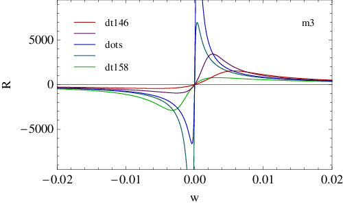
In fig. 30 we qualitatively sketch the result from the investigation of the behavior of the quasinormal modes closest to the origin of the complex $\mathfrak{w}$-plane. These modes do not produce the peaks corresponding to the spectrum (6.15).

Figure 30: A sketch of the positions and movements of the quasinormal modes under changes of $\tilde{d}$. Color indicates the function: $\text{red}=Y$, $\text{green}=X$, $\text{blue}=E^{3}$. The symbols indicate the range of $\tilde{d}$: $\circ<\tilde{d}_{\text{crit}}$, $\bullet=\tilde{d}_{\text{crit}}$, $\text{\tiny$\blacksquare$}>\tilde{d}_{\text{crit}}$. Poles in the gray region introduce instabilities.

At low densities all quasinormal modes are located in the lower half plane. When increasing the isospin density, the modes of the solutions $X$ and $Y$ to (6.20) and (6.21) move towards the origin of the frequency plane. At the same time two quasinormal modes of $E^{3}$ move towards each other and merge on the negative imaginary axis, then travel along the axis towards the origin as one single pole. At the critical value of $\tilde{d}$ the modes from $X$ and $Y$ meet at the origin, the quasinormal modes from $E^{3}$ still reside in the lower half plane. This observation matches the discussion below equations (6.20) to (6.22), where we expected $X$ and $Y$ to behave similarly at small $\mathfrak{w}$, while $E^{3}$ should differ from this behavior. Upon further increasing the isospin density, the modes $\Omega$ from $X$ and $Y$ enter the upper half plane, maintaining their distinct directions. The sign change in $\mathop{\mathrm{}}{Im}\Omega$ from $\mathop{\mathrm{}}{Im}\Omega<0$ to $\mathop{\mathrm{}}{Im}\Omega>0$ indicates that a damped resonance changes into a self-enhancing one, and thus introduces an instability to the system. Figure fig. 31 illustrates the transition of a quasinormal mode of $Y$ from the lower half plane to the upper half plane. The $E^{3}$-mode does not enter the upper half plane at any value of $\tilde{d}$ we considered. Compare this to the values of $\tilde{d}$ in fig. 27 and fig. 28 at which the pole induces visible structures at small $\mathfrak{w}$. A comparable movement of poles in a different but related setup was found in [65]. There the quasinormal modes of correlation functions of electromagnetic currents were investigated as a function of temperature.

Figure 31: Contour plot of the spectral function for $Y$ around $\mathfrak{w}=0$ in the complex $\mathfrak{w}$-plane. Left: $\tilde{d}=10<\tilde{d}_{\text{crit}}$, center: $\tilde{d}=15.352=\tilde{d}_{\text{crit}}$, right: $\tilde{d}=20.704>\tilde{d}_{\text{crit}}$. The three graphs where generated for $m=3$, dark shading indicates small values of $\mathfrak{R}$, light shading indicates large values. A pole in the upper half plane introduces an instability.

In the following we interpret the observation of decaying mesons and the emergence of a new peak in the spectral function in terms of field theory quantities. In particular we speculate on a new phase in the phase diagram for fundamental matter in the D$3$/D$7$ setup.

In the far UV, the field theory dual to our setup is supersymmetric, thus containing scalars as well as fermions, both of which contribute to the bound states we identified with mesons, even when supersymmetry is eventually broken. The meson decay at non-vanishing particle densities may be explained by the change of the shape of the potential for the scalars in the field theory upon the introduction of a non-vanishing density. As outlined in appendix C, a chemical potential may lead to an instability of the theory, since it induces a runaway potential for the scalar fields at small field values [66]. Nevertheless, interactions of $\phi^{4}$-type lead to a Mexican hat style potential for larger field values. In this way the theory is stabilized at finite density $\tilde{d}$ while the scalar fields condensate. This squark condensate presumably contributes to the vev of the scalar flavor current,

$$\tilde{d}\propto\left<J^{0}\right>\propto\left<\bar{\psi}\,\gamma^{0}\,\psi\right>+\left<\phi\;\partial^{0}\phi\right>.$$ (6.24)

In the AdS/CFT context the presence of an upside-down potential for the squark vev has been shown in [50] using an instanton configuration in the dual supergravity background.

The occurrence of a pole in the upper half plane of complex frequencies at finite $\tilde{d}_{\text{crit}}$ indicates an instability of the theory. A comparable observation was made in [48], where in fact the vector meson becomes unstable by means of negative values for its mass beyond some critical chemical potential. The difference between this work and [48] is that our model includes scalar modes in addition to the fundamental fermions. Nevertheless, in both models an instability occurs at a critical value of the chemical potential. The theory may still be stabilized dynamically by vector condensation [67]. In this case the system would enter a new phase of condensed vectors at densities larger than $\tilde{d}_{\text{crit}}$, in accordance with the expectation from QCD calculations [58, 59, 57].

We perform the analysis of the pole structure at $\mathfrak{w}=0$ for various $m$, and interpret the phenomenon of the transition of poles into the upper half plane at finite critical particle density as a sign of the transition to an unstable phase. We relate the critical particle density $\tilde{d}_{\text{crit}}$ to the according chemical potential $\tilde{\mu}^{I}$ by (2.37) and use the pairs of $m$ and critical dimensionful $\mu$ to trace the line of the phase transition in the phase diagram of fundamental matter in the D$3$/D$7$ setup. The result is drawn as a green line in fig. 32. The picture shows the $(\mu^{I},T)$-plane of the phase diagram and contains three regions, drawn as blue shaded, white, and green shaded, as well as a blue and a green line, separating the different regions.

Figure 32: The phase diagram for fundamental matter in the D$3$/D$7$ setup. In the blue shaded region D$7$-branes have the topology of Minkowski embeddings. The white and green regions are described by black hole embeddings. However, in the green region we interpret our observations as an instability of the black hole embeddings in the D$3$/D$7$ setup.

The blue shaded region marks the range of parameters, in which fundamental matter is described by D$7$-branes with Minkowski embeddings. The blue line, delimiting the the blue region, marks the line of phase transitions to the black hole phase, where fundamental matter is described by D$7$-branes which have black hole embeddings. This phase transition was discussed in section 4.2. Using the symmetries (2.33), this phase transition line can be mapped to the line of phase transitions between Minkowski and black hole embeddings, present at finite baryon chemical potential [28, 51, 68].

The green line and green shaded region in the phase diagram in fig. 32 mark the observation made in this section. The green line marks the values of $\tilde{d}_{\text{crit}}$ at which the pole in the spectral function appears at $\mathfrak{w}=0$. Beyond the green line we enter the green shaded unstable region.

We observe that the green line asymptotes to a straight line at high temperatures. Within the values computed by us, this line agrees with the asymptotic behavior of the contour of particle density with $\tilde{d}\approx 20.5$, drawn as a gray line in the phase diagram. We thus speculate on a finite critical particle density beyond which the black hole phase is unstable. This interpretation is supported by analogous studies of the phase diagram of $\mathcal{N}=4$ super-Yang-Mills theory with R-symmetry chemical potentials, where a similar line in the phase diagram was discovered [45, 56]. Up to now it is unclear whether the new phase indeed is unstable or if it only indicates that black hole embeddings are not capable of describing this state of matter.

Note that the location of the green phase transition line in fig. 32 as well as the results shown in fig. 31 and fig. 30 are obtained from the analysis of poles in the spectral functions. These functions in turn are obtained as solutions to equations (6.20) to (6.22), which do depend on the so far unknown factor $c$ in (6.23). The computation of this factor is left to future work. It will determine the exact position of the green phase transition line in fig. 32. This will answer the question whether there is a triple point in the phase diagram and if the blue and green shaded regions meet at a common border. Moreover, other poles than the ones investigated here may have influence on the stability of this system.

7 Conclusion

In this work we have considered a probe of $N_{f}$ D7 branes embedded in the AdS Schwarzschild black hole background with an $U(N_{f})$ gauge field. This configuration is conjectured to be dual to a thermal quantum field theory with isospin and baryon charge. We have considered both the canonical and grand canonical ensemble. Our detailed study of this background provides a basis for further studies. For instance it is now possible to investigate the mesonic excitation spectrum or hydrodynamic properties in detail.

By including isospin density, we find four new phase boundaries coincident with the fixed points of the accidental symmetries between baryon and isospin density, which our setup displays. Along the lines of equal densities $|\tilde{d}^{B}|=|\tilde{d}^{I}|$ and near $T=0$, we find a sharp transition in the chemical potentials. This situation is reminiscent of a corresponding transition found in two-color QCD [46]. For $T=0$ the chemical potential is discontinuous and a one-to-one correspondence between the thermodynamic conjugate variables $\tilde{d}$ and $\tilde{\mu}$ can not be established. This inconsistency between the two ensembles signals an instability of the setup in that phase region. We expect that vector mesons condense in this region as is also expected in QCD [46]. A further detailed study of this new phase requires the investigation of scalar and pseudoscalar fluctuations as well. Furthermore, an analysis of the possible condensates is required, cf. [48]. This is a promising task for future investigation. It would also be interesting to study the heat capacity and the quasi-particle spectrum at low temperature as in [69] in the more general setup provided in this paper. This study may give a better understanding of the new quantum liquid found in [69].

Here we have restricted to vector fluctuations about the finite isospin density background. Analyzing these fluctuations, we found an unstable region in the $(\mu^{I},\,T)$ phase diagram which is bounded by a line of constant density. We expect that mesons condense in this unstable phase. The emerging phase structure appears to be a generic feature of holographic duals with chemical potentials as a similar behavior has been observed for spinning branes [70] and R-charged black hole backgrounds [56, 71]. It would be interesting to shed more light on the connection between the new phase found in this work and in the backgrounds mentioned above.

Considering the effective baryon diffusion, we find competing behavior between baryon and isospin density. For example at a given temperature, increasing $\tilde{d}^{B}$ increases the effective baryon diffusion while increasing $\tilde{d}^{I}$ suppresses that diffusion. Note that this effective baryon density collects both, the effect of finite baryon and of finite isospin density on the effective baryon diffusion. It would be very interesting to separate these two contributions, for example by a modification of the membrane paradigm.

All the numerical results mentioned here were obtained for $N_{f}=2$. However, they may also be generated for arbitrary $N_{f}\ll N_{c}$ from the general expressions we have provided here.

Appendix A Simplification of the DBI action

In this section we give some details for the simplifications done in the equations (2.21), (2.22), (2.23). We argued that the square root in the action (2.21) is diagonal in flavor space and the DBI action decouple for the fields defined in (2.22). To prove this, we first have to calculate the square of the non-vanishing field strength component $(F_{40})^{2}$. For this calculation we need some multiplication relations for the matrices $\lambda^{i}$ given by

$$\begin{split}\lambda^{1}\lambda^{i}&=\lambda^{i}\quad i=1,\dots,N_{f}\\ (\lambda^{i})^{2}&=\mathrm{diag}(1,\dots,\overbrace{(N_{f}-1)^{2}}^{i\text{-th position}},\dots,1)\quad i=2,\dots,N_{f}\\ \lambda^{i}\lambda^{j}&=\mathrm{diag}(1,\dots,\overbrace{-(N_{f}-1)}^{i\text{-th position}},\dots,\overbrace{-(N_{f}-1)}^{j\text{-th position}},\dots,1)\quad i\not=j\end{split}$$ (A.1)

and the fact that all matrices $\lambda^{i}$ commute with each other since they are the generators of the Cartan subalgebra. The $i$-th diagonal component of the matrix $(F_{40})^{2}$ is then for $i=1$

$$\begin{split}\left((F_{40})^{2}\right)_{11}&=\left[\sum_{j=1}^{N_{f}}(F^{I_{j}}_{40})^{2}(\lambda^{j})^{2}+2\sum_{j=2}^{N_{f}}F^{I_{1}}_{40}F^{I_{j}}_{40}\lambda^{1}\lambda^{j}+2\sum_{j=2}^{N_{f}}\sum_{\begin{subarray}{c}k=2\\ k\not=j\end{subarray}}^{N_{f}}F^{I_{j}}_{40}F^{I_{k}}_{40}\lambda^{j}\lambda^{k}\right]_{11}\\ &=\left(\sum_{j=1}^{N_{f}}F^{I_{j}}_{40}\right)^{2}=(\partial_{\varrho}X_{1})^{2}\end{split}$$ (A.2)

and for $i\not=1$

$$\begin{split}\left((F_{40})^{2}\right)_{ii}=&\Bigg[\sum_{\begin{subarray}{c}j=1\\ j\not=i\end{subarray}}^{N_{f}}(F^{I_{j}}_{40})^{2}(\lambda^{j})^{2}+(F^{I_{i}}_{40})^{2}(\lambda^{i})^{2}+2\sum_{\begin{subarray}{c}j=1\\ j\not=i\end{subarray}}F^{I_{i}}_{40}F^{I_{j}}_{40}\lambda^{i}\lambda^{j}\\ &+2\sum_{j=1}^{N_{f}}\sum_{\begin{subarray}{c}k=1\\ k\not=i\end{subarray}}^{N_{f}}F^{I_{j}}_{40}F^{I_{k}}_{40}\lambda^{j}\lambda^{k}\Bigg]_{ii}\\ =&\left(\sum_{\begin{subarray}{c}j=1\\ j\not=i\end{subarray}}^{N_{f}}F^{I_{j}}_{40}-(N_{f}-1)F^{I_{i}}_{40}\right)^{2}=(\partial_{\varrho}X_{i})^{2}\,,\end{split}$$ (A.3)

where we used the new fields as defined in equation (2.22) in the last equalities. With this choice of the new fields and since $F_{40}$ is diagonal in the flavor space, each component of the diagonal is given by the expression known from the pure baryonic case [27]

$$\begin{split}\left(\sqrt{\lambda^{1}+(2\pi\alpha^{\prime})^{2}G^{00}G^{44}(F_{40})^{2}}\right)_{ii}&=\sqrt{1+(2\pi\alpha^{\prime})^{2}G^{00}G^{44}((F_{40})^{2})_{ii}}\\ &=\sqrt{1+(2\pi\alpha^{\prime})^{2}G^{00}G^{44}(\partial_{\varrho}X_{i})^{2}}\,.\end{split}$$ (A.4)

Taking the trace and simplifying the expressions of the metric factors, we get equation (2.23).

Appendix B Effect of the accidental symmetries for $N_{f}=3$

In this section we give the action of the accidental symmetries discussed in section 2.3.1 in the physical basis for $N_{f}=3$:

$$d_{1} \leftrightarrow d_{2}: d^{B}\mapsto d^{B} d^{I_{2}}\mapsto-(d^{I_{2}}+d^{I_{3}}) d^{I_{3}}\mapsto d^{I_{3}}$$ (B.1)

$$d_{1} \leftrightarrow d_{3}: d^{B}\mapsto d^{B} d^{I_{2}}\mapsto d^{I_{2}} d^{I_{3}}\mapsto-(d^{I_{2}}+d^{I_{3}})$$

$$d_{2} \leftrightarrow d_{3}: d^{B}\mapsto d^{B} d^{I_{2}}\mapsto d^{I_{3}} d^{I_{3}}\mapsto d^{I_{2}}$$

$$d_{1} \leftrightarrow-d_{1}:\hskip 14.72241pt d^{B}\mapsto\frac{1}{3}(d^{B}-2d^{I_{2}}-2d^{I_{3}})\hskip 14.72241pt d^{I_{2}}\mapsto\frac{1}{3}(-2d^{B}+d^{I_{2}}-2d^{I_{3}})\hskip 14.72241pt d^{I_{3}}\mapsto\frac{1}{3}(-2d^{B}-2d^{I_{2}}+d^{I_{3}})$$

$$d_{2} \leftrightarrow-d_{2}: d^{B}\mapsto\frac{1}{3}(d^{B}+2d^{I_{2}}) d^{I_{2}}\mapsto\frac{1}{3}(4d^{B}-d^{I_{2}}) d^{I_{3}}\mapsto\frac{1}{3}(-2d^{B}+2d^{I_{2}}+d^{I_{3}})$$

$$d_{3} \leftrightarrow-d_{3}: d^{B}\mapsto\frac{1}{3}(d^{B}+2d^{I_{3}}) d^{I_{2}}\mapsto\frac{1}{3}(-2d^{B}+d^{I_{2}}+2d^{I_{3}}) d^{I_{3}}\mapsto\frac{1}{3}(4d^{B}-d^{I_{3}})\,.$$

Since the transformation matrix to the physical basis for $N_{f}=3$ is not an orthogonal matrix, there is no induced approximate $O(3)$ symmetry in the physical basis. This is in general also true for all cases with $N_{f}\geq 3$.

Appendix C Chemical potentials in field theories: Runaway potential and Bose-Einstein Condensation

In our setup we consider a theory which is supersymmetric in the far UV. Its fundamental matter consists of complex scalars (squarks) and fermionic fields (quarks). In this section we describe the effect of the chemical potential on the field theory Lagrangian and on the vacuum as e. g. in [66]. We consider a theory with one complex scalar $\phi$ and one fermionic field $\psi$ with the same mass $M_{q}$ coupled to an $U(1)$ gauge field $A_{\nu}$. The time component of the $U(1)$ gauge field has a non-zero vev which induces the chemical potential $\mu$,

$$A_{\nu}=\mu\delta_{\nu 0}\,.$$ (C.1)

The Lagrangian is given by

$${\cal L}=-D_{\nu}\phi^{*}D^{\nu}\phi-M_{q}^{2}\phi^{*}\phi-\bar{\psi}(D\hskip-11.0pt\diagup+M_{q})\psi-\frac{1}{4}F_{\mu\nu}F^{\mu\nu}\,,$$ (C.2)

where $D_{\nu}=\partial_{\nu}-{\mathrm{i}}A_{\nu}$ is the covariant derivative and $F_{\mu\nu}=\partial_{\mu}A_{\nu}-\partial_{\nu}A_{\mu}$ the field strength tensor. Expanding the Lagrangian around the non-zero vev of the gauge field, the Lagrangian becomes

$${\cal L}=-\partial_{\nu}\phi^{*}\partial^{\nu}\phi-(M_{q}^{2}-\mu^{2})\phi^{*}\phi+\mu J^{s}_{0}-\bar{\psi}(\partial\hskip-7.0pt\diagup+M_{q})\psi+\mu J_{0}^{F}\,,$$ (C.3)

where $J^{S}_{\mu}={\mathrm{i}}[(\partial_{\mu}\phi^{*})\phi-\phi^{*}(\partial_{\mu}\phi)]$, $\left(J^{\mu}\right)^{F}=-{\mathrm{i}}\bar{\psi}\gamma^{\mu}\psi$ are conserved currents. These conserved currents are the population density for the scalar $N_{S}$ and fermionic fields $N_{F}$, such that the linear terms in the Lagrangian are $\mu N_{S}$ and $\mu N_{F}$.

The mass term $-(M_{q}^{2}-\mu^{2})\phi^{2}$ of the Lagrangian (C.3) introduces an instability if $\mu>M_{q}$ since the corresponding potential $V=(M_{q}^{2}-\mu^{2})\phi^{2}+\cdots$ is not bounded from below. In some systems this runaway potential is stabilized by higer interactions and becomes a Mexican hat potential such that the scalar condense and the scalar density becomes non-zero. This condensation is known as Bose-Einstein-Condensation.

Appendix D Coupling constant for vector meson interaction

In this section we show how the coupling constant for the interaction of vector mesons can be computed, extending the ideas presented in [44]. This coupling constant in the effective four-dimensional meson theory can be determined by redefinition of the gauge fields such that the kinetic term has canonical form. This coupling constant depends on the geometry of the extra dimensions.

First we consider the eight-dimensional theory determined by the DBI action $S^{(2)}_{\text{DBI}}$ expanded to second order in the fluctuations $\tilde{A}$,

$$S^{(2)}_{\text{DBI}}=\frac{T_{D7}(2\pi\alpha^{\prime})^{2}}{4}\int\!\mathrm{d}^{8}\xi\sqrt{-G}\;G^{\mu\mu^{\prime}}G^{\nu\nu^{\prime}}F_{\mu^{\prime}\nu}F_{\nu^{\prime}\mu}\,,$$ (D.1)

where $G$ contains the background fields and we simplify the analysis by considering only Abelian gauge fields. Defining the dimensionless coordinate $\rho=\varrho/R$ and integrating out the contribution of the $S^{3}$, we obtain

$$S^{(2)}_{\text{DBI}}=\frac{T_{D_{7}}(2\pi\alpha^{\prime})^{2}\text{vol}(S_{3})R^{4}}{4}\int\!\mathrm{d}^{4}x\int\!\mathrm{d}\rho\sqrt{-G}\;G^{\mu\mu^{\prime}}G^{\mu\nu^{\prime}}F_{\mu^{\prime}\nu}F_{\nu^{\prime}\mu}\,.$$ (D.2)

To obtain a four-dimensional effective theory we have to integrate over the coordinate $\rho$. This contribution depends on the geometry induced by the $\rho$ dependence of the metric factors. However, we expect that it is independent of the ’t Hooft coupling $\lambda$. We parametrize this contribution by $c^{\prime}$. The kinetic term of the effective theory is then given by

$$S^{(2)}_{\text{DBI}}=\frac{T_{D7}(2\pi\alpha^{\prime})^{2}\text{vol}(S_{3})R^{4}c^{\prime}}{4}\int\!\mathrm{d}^{4}x\;F_{\mu\nu}F^{\mu\nu}\,,$$ (D.3)

where the prefactor may be written as

$$\frac{T_{D7}(2\pi\alpha^{\prime})^{2}\text{vol}(S_{3})R^{4}c^{\prime}}{4}=\frac{\lambda}{g_{\text{YM}}^{2}c^{2}}\,,$$ (D.4)

where the numerical values independent of the ’t Hooft coupling are grouped into the coefficient $c$. From this we can read off that a rescaling of the form

$$A\mapsto\frac{c}{\sqrt{\lambda}}A$$ (D.5)

casts the Lagrangian into canonical form with a prefactor of $1/g_{\text{YM}}^{2}$.

References

- [1] J. M. Maldacena, The large N limit of superconformal field theories and supergravity, Adv. Theor. Math. Phys. 2 (1998) 231–252, arXiv:hep-th/9711200.
- [2] O. Aharony, S. S. Gubser, J. M. Maldacena, H. Ooguri, and Y. Oz, Large N field theories, string theory and gravity, Phys. Rept. 323 (2000) 183–386, arXiv:hep-th/9905111.
- [3] E. Witten, Anti-de Sitter space, thermal phase transition, and confinement in gauge theories, Adv. Theor. Math. Phys. 2 (1998) 505–532, arXiv:hep-th/9803131.
- [4] D. T. Son and A. O. Starinets, Viscosity, Black Holes, and Quantum Field Theory, Ann. Rev. Nucl. Part. Sci. 57 (2007) 95–118, arXiv:0704.0240.
- [5] G. Policastro, D. T. Son, and A. O. Starinets, The shear viscosity of strongly coupled N = 4 supersymmetric Yang-Mills plasma, Phys. Rev. Lett. 87 (2001) 081601, arXiv:hep-th/0104066.
- [6] G. Policastro, D. T. Son, and A. O. Starinets, From AdS/CFT correspondence to hydrodynamics, JHEP 09 (2002) 043, arXiv:hep-th/0205052.
- [7] G. Policastro, D. T. Son, and A. O. Starinets, From AdS/CFT correspondence to hydrodynamics. II: Sound waves, JHEP 12 (2002) 054, arXiv:hep-th/0210220.
- [8] C. P. Herzog, The hydrodynamics of M-theory, JHEP 12 (2002) 026, arXiv:hep-th/0210126.
- [9] C. P. Herzog, The sound of M-theory, Phys. Rev. D68 (2003) 024013, arXiv:hep-th/0302086.
- [10] P. Kovtun, D. T. Son, and A. O. Starinets, Holography and hydrodynamics: Diffusion on stretched horizons, JHEP 10 (2003) 064, arXiv:hep-th/0309213.
- [11] A. Buchel and J. T. Liu, Universality of the shear viscosity in supergravity, Phys. Rev. Lett. 93 (2004) 090602, arXiv:hep-th/0311175.
- [12] P. Kovtun, D. T. Son, and A. O. Starinets, Viscosity in strongly interacting quantum field theories from black hole physics, Phys. Rev. Lett. 94 (2005) 111601, arXiv:hep-th/0405231.
- [13] A. Buchel, J. T. Liu, and A. O. Starinets, Coupling constant dependence of the shear viscosity in N=4 supersymmetric Yang-Mills theory, Nucl. Phys. B707 (2005) 56–68, arXiv:hep-th/0406264.
- [14] P. Benincasa, A. Buchel, and A. O. Starinets, Sound waves in strongly coupled non-conformal gauge theory plasma, Nucl. Phys. B733 (2006) 160–187, arXiv:hep-th/0507026.
- [15] J. Mas, Shear viscosity from R-charged AdS black holes, JHEP 03 (2006) 016, arXiv:hep-th/0601144.
- [16] D. T. Son and A. O. Starinets, Hydrodynamics of R-charged black holes, JHEP 03 (2006) 052, arXiv:hep-th/0601157.
- [17] K. Maeda, M. Natsuume, and T. Okamura, Viscosity of gauge theory plasma with a chemical potential from AdS/CFT, Phys. Rev. D73 (2006) 066013, arXiv:hep-th/0602010.
- [18] C. P. Herzog, Energy loss of heavy quarks from asymptotically AdS geometries, JHEP 09 (2006) 032, arXiv:hep-th/0605191.
- [19] J. Casalderrey-Solana and D. Teaney, Heavy quark diffusion in strongly coupled N = 4 Yang Mills, Phys. Rev. D74 (2006) 085012, arXiv:hep-ph/0605199.
- [20] A. Buchel, Shear viscosity of CFT plasma at finite coupling, Phys. Lett. B665 (2008) 298–304, arXiv:0804.3161.
- [21] R. C. Myers, M. F. Paulos, and A. Sinha, Quantum corrections to eta/s, arXiv:0806.2156.
- [22] A. Karch and E. Katz, Adding flavor to AdS/CFT, JHEP 06 (2002) 043, arXiv:hep-th/0205236.
- [23] J. Babington, J. Erdmenger, N. J. Evans, Z. Guralnik, and I. Kirsch, Chiral symmetry breaking and pions in non-supersymmetric gauge / gravity duals, Phys. Rev. D69 (2004) 066007, arXiv:hep-th/0306018.
- [24] I. Kirsch, Generalizations of the AdS/CFT correspondence, Fortsch. Phys. 52 (2004) 727–826, arXiv:hep-th/0406274.
- [25] D. Mateos, R. C. Myers, and R. M. Thomson, Thermodynamics of the brane, JHEP 05 (2007) 067, arXiv:hep-th/0701132.
- [26] M. Kruczenski, D. Mateos, R. C. Myers, and D. J. Winters, Towards a holographic dual of large-N(c) QCD, JHEP 05 (2004) 041, arXiv:hep-th/0311270.
- [27] S. Kobayashi, D. Mateos, S. Matsuura, R. C. Myers, and R. M. Thomson, Holographic phase transitions at finite baryon density, JHEP 02 (2007) 016, arXiv:hep-th/0611099.
- [28] D. Mateos, S. Matsuura, R. C. Myers, and R. M. Thomson, Holographic phase transitions at finite chemical potential, JHEP 11 (2007) 085, arXiv:0709.1225.
- [29] S. Nakamura, Y. Seo, S.-J. Sin, and K. P. Yogendran, A new phase at finite quark density from AdS/CFT, J. Korean Phys. Soc. 52 (2008) 1734–1739, arXiv:hep-th/0611021.
- [30] S. Nakamura, Y. Seo, S.-J. Sin, and K. P. Yogendran, Baryon-charge Chemical Potential in AdS/CFT, Prog. Theor. Phys. 120 (2008) 51–76, arXiv:0708.2818.
- [31] K. Ghoroku, M. Ishihara, and A. Nakamura, D3/D7 holographic Gauge theory and Chemical potential, Phys. Rev. D76 (2007) 124006, arXiv:0708.3706.
- [32] K.-Y. Kim, S.-J. Sin, and I. Zahed, Dense hadronic matter in holographic QCD, arXiv:hep-th/0608046.
- [33] N. Horigome and Y. Tanii, Holographic chiral phase transition with chemical potential, JHEP 01 (2007) 072, arXiv:hep-th/0608198.
- [34] D. T. Son and A. O. Starinets, Minkowski-space correlators in AdS/CFT correspondence: Recipe and applications, JHEP 09 (2002) 042, arXiv:hep-th/0205051.
- [35] C. P. Herzog and D. T. Son, Schwinger-Keldysh propagators from AdS/CFT correspondence, JHEP 03 (2003) 046, arXiv:hep-th/0212072.
- [36] C. Hoyos-Badajoz, K. Landsteiner, and S. Montero, Holographic Meson Melting, JHEP 04 (2007) 031, arXiv:hep-th/0612169.
- [37] C. Hoyos-Badajoz, K. Landsteiner, and S. Montero, Quasinormal modes and meson decay rates, Fortsch. Phys. 55 (2007) 760–764.
- [38] I. Amado, C. Hoyos-Badajoz, K. Landsteiner, and S. Montero, Residues of Correlators in the Strongly Coupled N=4 Plasma, Phys. Rev. D77 (2008) 065004, arXiv:0710.4458.
- [39] R. C. Myers, A. O. Starinets, and R. M. Thomson, Holographic spectral functions and diffusion constants for fundamental matter, JHEP 11 (2007) 091, arXiv:0706.0162.
- [40] D. Mateos and L. Patino, Bright branes for strongly coupled plasmas, JHEP 11 (2007) 025, arXiv:0709.2168.
- [41] R. C. Myers and A. Sinha, The fast life of holographic mesons, arXiv:0804.2168.
- [42] J. Mas, J. P. Shock, J. Tarrio, and D. Zoakos, Holographic Spectral Functions at Finite Baryon Density, arXiv:0805.2601.
- [43] J. Erdmenger, M. Kaminski, and F. Rust, Holographic vector mesons from spectral functions at finite baryon or isospin density, Phys. Rev. D77 (2008) 046005, arXiv:0710.0334.
- [44] M. Kruczenski, D. Mateos, R. C. Myers, and D. J. Winters, Meson spectroscopy in AdS/CFT with flavour, JHEP 07 (2003) 049, arXiv:hep-th/0304032.
- [45] D. Yamada and L. G. Yaffe, Phase diagram of N = 4 super-Yang-Mills theory with R- symmetry chemical potentials, JHEP 09 (2006) 027, arXiv:hep-th/0602074.
- [46] K. Splittorff, D. T. Son, and M. A. Stephanov, QCD-like theories at finite baryon and isospin density, Phys. Rev. D64 (2001) 016003, arXiv:hep-ph/0012274.
- [47] K. Binder, Theory of first-order phase transitions, Reports on Progress in Physics 50 (1987), no. 7, 783–859.
- [48] O. Aharony, K. Peeters, J. Sonnenschein, and M. Zamaklar, Rho meson condensation at finite isospin chemical potential in a holographic model for QCD, JHEP 02 (2008) 071, arXiv:0709.3948.
- [49] J. Erdmenger, M. Kaminski, and F. Rust, Isospin diffusion in thermal AdS/CFT with flavor, Phys. Rev. D76 (2007) 046001, arXiv:0704.1290.
- [50] R. Apreda, J. Erdmenger, N. Evans, and Z. Guralnik, Strong coupling effective Higgs potential and a first order thermal phase transition from AdS/CFT duality, Phys. Rev. D71 (2005) 126002, arXiv:hep-th/0504151.
- [51] A. Karch and A. O’Bannon, Holographic Thermodynamics at Finite Baryon Density: Some Exact Results, JHEP 11 (2007) 074, arXiv:0709.0570.
- [52] A. Karch, A. O’Bannon, and K. Skenderis, Holographic renormalization of probe D-branes in AdS/CFT, JHEP 04 (2006) 015, arXiv:hep-th/0512125.
- [53] L. D. Landau and E. M. Lifshitz, Course of Theoretical Physics, Volume 5, Statistical Physics ,. Pergamon Press (1980) 544p.
- [54] A. H. Marshall, B. Chakraborty, and S. Nagel, Numerical studies of the compressible Ising spin glass, Europhysics Letters 74 (may, 2006) 699–705.
- [55] E. A. Uehling, Polarization Effects in the Positron Theory, Phys. Rev. 48 (Jul, 1935) 55–63.
- [56] M. Cvetic and S. S. Gubser, Phases of R-charged black holes, spinning branes and strongly coupled gauge theories, JHEP 04 (1999) 024, arXiv:hep-th/9902195.
- [57] D. N. Voskresensky, On the possibility of the condensation of the charged rho meson field in dense isospin asymmetric baryon matter, Phys. Lett. B392 (1997) 262–266.
- [58] J. T. Lenaghan, F. Sannino, and K. Splittorff, The superfluid and conformal phase transitions of two- color QCD, Phys. Rev. D65 (2002) 054002, arXiv:hep-ph/0107099.
- [59] F. Sannino, General structure of relativistic vector condensation, Phys. Rev. D67 (2003) 054006, arXiv:hep-ph/0211367.
- [60] D. T. Son and M. A. Stephanov, QCD at finite isospin density: From pion to quark antiquark condensation, Phys. Atom. Nucl. 64 (2001) 834–842, arXiv:hep-ph/0011365.
- [61] D. T. Son and M. A. Stephanov, QCD at finite isospin density, Phys. Rev. Lett. 86 (2001) 592–595, arXiv:hep-ph/0005225.
- [62] D. Ebert, K. G. Klimenko, A. V. Tyukov, and V. C. Zhukovsky, Pion condensation of quark matter in the static Einstein universe, arXiv:0804.0765.
- [63] L.-y. He, M. Jin, and P.-f. Zhuang, Pion superfluidity and meson properties at finite isospin density, Phys. Rev. D71 (2005) 116001, arXiv:hep-ph/0503272.
- [64] A. Paredes, K. Peeters, and M. Zamaklar, Mesons versus quasi-normal modes: undercooling and overheating, JHEP 05 (2008) 027, arXiv:0803.0759.
- [65] S. S. Gubser and S. S. Pufu, The gravity dual of a p-wave superconductor, arXiv:0805.2960.
- [66] R. Harnik, D. T. Larson, and H. Murayama, Supersymmetric color superconductivity, JHEP 03 (2004) 049, arXiv:hep-ph/0309224.
- [67] A. Buchel, J. Jia, and V. A. Miransky, Dynamical stabilization of runaway potentials at finite density, Phys. Lett. B647 (2007) 305–308, arXiv:hep-th/0609031.
- [68] J. Erdmenger, N. Evans, I. Kirsch, and E. Threlfall, Mesons in Gauge/Gravity Duals - A Review, Eur. Phys. J. A35 (2008) 81–133, arXiv:0711.4467.
- [69] A. Karch, D. T. Son, and A. O. Starinets, Zero Sound from Holography, arXiv:0806.3796.
- [70] S. S. Gubser, Thermodynamics of spinning D3-branes, Nucl. Phys. B551 (1999) 667–684, arXiv:hep-th/9810225.
- [71] D. Yamada, Metastability of R-charged black holes, Class. Quant. Grav. 24 (2007) 3347–3376, arXiv:hep-th/0701254.