MAD-TH-08-10

CERN-PH-TH/2008-146

Systematics of Multi-field Effects

at the End of Warped Brane Inflation

Heng-Yu Chen¹, Jinn-Ouk Gong¹, and Gary Shiu^1,2

¹Department of Physics, University of Wisconsin-Madison, Madison, WI 53706-1390, USA

²PH-TH Division, CERN, CH-1211 Geneva 23, Switzerland

Abstract

We investigate in the context of brane inflation the possibility of additional light scalar fields generating significant power spectrum and non-Gaussianities at the end of inflation affecting the CMB scale observations. We consider the specific mechanism outlined by Lyth and describe the necessary criteria for it to be potentially important in a warped throat. We also discuss different mechanisms for uplifting the vacuum energy which can lead to different dominant contributions of the inflaton potential near the end of inflation. We then apply such criteria to one of the most detailed brane inflation models to date, and show that inflation can persist towards the tip of the throat, however for the specific stable inflationary trajectory, the light residual isometry direction becomes degenerate. We also estimate the effects for other inflationary trajectories with non-degenerate residual isometries.

August 24, 2026

1 Introduction

Inflation [1] has emerged as the standard paradigm describing physics of the very early universe. Besides addressing several fine-tuning issues in big bang cosmology such as the flatness and horizon problems, it provides a framework to explain the origin of structure and the cosmic microwave background (CMB) anisotropy [2]. While there is a plethora of effective field theory based models of inflation [3], many outstanding questions in inflationary cosmology require a fundamental microscopic description. Conversely, recent observations of the CMB and large scale structure [4] lead us to increasingly precise measurements of the inflationary parameters. These measurements provide us with an exciting window to probe physics at ultra-high energies [5], far higher than what current and upcoming terrestrial accelerators can reach. Thus inflationary cosmology has become the perfect arena for fundamental theory to meet experiment.

String theory is currently our leading candidate for a quantum theory of gravity. Thus it is worthwhile to explore explicit realizations of inflation within this framework. In this paper, we will focus on one of the most well developed inflationary scenarios in string theory, i.e. $D$ brane inflation [6] (see also Refs. [7, 8]; for reviews, see Ref. [9] and references therein), where the inflaton field is identified with the position of a space-filling mobile $D$ brane, usually a $D3$ brane, in a warped six dimensional manifold [10]. In the original scenario of Refs. [6, 7, 8, 9, 10], an additional $\overline{D3}$ was introduced to drive inflation. The $\overline{D3}$ brane is localized by the RR fluxes at the tip of a warped throat, thus inflation proceeds as the mobile $D3$ is attracted by a weak $D3$-$\overline{D3}$ Coulombic force to move slowly along the warped direction. However, it was also noted in Ref. [10] that because the volume modulus of the compactification couples non-trivially to the canonical inflaton, its stabilized value gives additional Hubble scale correction to the inflaton mass, causing the well known $\eta$ problem [11].

An important step towards addressing the $\eta$ problem explicitly in this concrete setting was recently made in Refs. [12, 13] (see also Refs. [14, 15, 16, 17]). The key ingredient in the construction was the one loop threshold correction to the non-perturbative superpotential obtained in Ref. [18] (see also Refs. [19, 20]). In Ref. [21] and other stabilized compactifications, non-perturbative effects are often introduced to stabilize moduli. In the context of Ref. [21], such effects come from instantons on a stack of $D7$ branes (or Euclidean $D3$ branes). Interestingly, the non-perturbative moduli stabilizing force also turns out to give the dominant contribution to the inflaton potential. This contribution arises because the mobile $D3$ brane backreacts on the moduli stabilizing $D7$ branes. The correction depends on the holomorphic four cycles within the conifold on which the $D7$ branes wrap. The embedding of the $D7$ branes breaks the isometry of the deformed conifold, and thus the inflationary trajectory depends sensitively on the choice of the embedding function defining the loci of the $D7$ branes. As a result, explicit slow-roll models have been constructed by a “delicate” tuning of the microscopic compactification parameters.

While the broken angular isometry directions are stabilized by the coordinate dependent non-perturbative superpotential, for a given $D7$ brane embedding, there are typically residual isometries preserved by the resultant scalar potential. The potential for the fields associated with these isometries remain flat during the inflationary epoch and so they can take arbitrary values without affecting the inflationary trajectory. Being almost massless, their quantum fluctuations give rise to a nearly scale invariant isocurvature perturbation spectrum. As argued by Lyth and collaborators in Refs. [22, 23], these isocurvature perturbations can be converted to the curvature perturbations at the end of inflation. In the context of $D$ brane inflation, inflation ends when the open string tachyon condenses between the mobile $D3$ and $\overline{D3}$. The critical value of the canonical inflaton at which inflation ends $\phi_{\rm end}$ depends on the residual symmetries as they enter into the tachyon potential. Since $\phi_{\rm end}$ picks up spatial dependence through the quantum fluctuations of the light residual symmetries, inflation can end on a spatial slice of non-uniform energy density. As we will see, this is the case for instance when the inflaton potential is dominated by the moduli stabilizing force towards the end of inflation. Thus, one could in principle expect potentially significant contribution to the power spectrum and non-Gaussianities at the end of inflation.

In this paper, we study these multi-field effects at the end of brane inflation, and outline the necessary conditions for them to be significant. We then perform a case study for the setup considered in Ref. [13], by explicitly calculating the canonical inflaton potential near the tip of the deformed conifold, and demonstrate that inflation can persist in this region provided that the $D3$-$\overline{D3}$ Coulombic attraction becomes subdominant. We also discuss various mechanisms to uplift the vacuum energy which results in a subdominant Coulombic potential all the way to the tip of a warped throat. We also show that the angular stable inflationary trajectory for the specific $D7$ brane embedding [24] used in Ref. [13] can be extended to the entire deformed conifold. However, along the specific trajectory considered in Ref. [13], we will see explicitly that the corresponding residual angular isometries have vanishing proper separations at the tip. Thus, for this specific $D7$ embedding, no significant contribution to the curvature perturbation is generated at the end of inflation. This implies that while multi-field effects can in principle be significant in brane inflation, they can only happen with other $D7$ embeddings, or with more than one stacks of $D7$ branes present.

This paper is organized as follows. In Section 2, we review the basic setup of flux compactification and brane inflation, in order to set up our notation. Readers who are familiar with the above topics can skip this section. In Section 3, we recast the mechanism proposed in Ref. [22] in the context of brane inflation in a warped throat, and outline the necessary conditions for it to take place. In Section 4, we discuss various possible uplifting mechanisms in a warp throat and propose a natural scenario for an uplifted potential to realize the effect of Ref. [22]. In Section 5, we explicitly calculate the canonical inflaton potential near the tip of the deformed conifold and the resulting slow-roll parameters. The degeneracy of the residual isometries will also be shown. We end with some discussions in Section 6. We relegate most of the calculational details in a number of Appendices.

2 $D3$ brane in warped compactifications

We will consider warped compactification of type IIB string theory in four dimensions [25] (see also earlier works on warped IIB vacua [26, 27, 28]), with the following metric ansatz

$$ds^{2}=e^{2A(y)}e^{-6u(x)}g_{\mu\nu}dx^{\mu}dx^{\nu}+e^{-2A(y)}e^{2u(x)}\tilde{g}_{mn}dy^{m}dy^{n}\,,$$ (2.1)

where $e^{A(y)}$ is the warp factor sourced by branes and fluxes, and $e^{u(x)}$ is the Weyl rescaling factor required to decouple the overall volume modulus from the four dimensional graviton, which can be taken as ${\mathcal{O}}(1)$. The internal metric $\tilde{g}_{mn}$ is taken to be that of a compact six dimensional Calabi-Yau space. In addition to the ansatz (2.1), we choose the bulk RR and NS-NS fluxes of type IIB supergravity to respect four dimensional Lorentz invariance (and self-duality in the case of the five form flux),

$$G_{3} \equiv F_{3}-\tau H_{3}=\frac{1}{6}G_{mnp}\ dy^{m}\wedge dy^{n}\wedge dy^{p}\,,$$ (2.2)

$$\widetilde{F}_{5} =(1+*)d\alpha(y)\wedge\sqrt{|g_{4}|}dx^{0}\wedge dx^{1}\wedge dx^{2}\wedge dx^{3}\,,$$ (2.3)

where we combined the NS-NS and RR three forms $H_{3}$ and $F_{3}$ with the complex axio-dilaton $\tau\equiv C_{0}+ie^{-\phi}$ into the complex combination $G_{3}$.

We are interested in the background BPS solutions of the equations of motion which impose the following relations on the fluxes [25],

$$\alpha(y) =e^{4A(y)}\,,$$ (2.4)

$$*_{6}G_{3} =iG_{3}\,,$$ (2.5)

such that the complexified three form flux is imaginary self-dual.

2.1 Four dimensional effective theory

At energy scales much lower than the Kaluza-Klein mass scale, the effective theory for this warped background is described by four dimensional $\mathcal{N}=1$ supergravity. The scalar fields of our theory consist of closed string moduli, including the complex structure moduli, axio-dilaton and Kähler moduli, as well as open string moduli, such as the positions of $D3$ branes and $D7$ branes. The flux-induced superpotential [29]

$$W_{\mathrm{GVW}}=\int G_{3}\wedge\Omega$$ (2.6)

stabilizes the complex structure moduli and axio-dilaton as described in Ref. [25], where $\Omega$ is the holomorphic $(3,0)$ form of the unwarped Calabi-Yau space. Lifting (2.6) to F-theory, we see that bulk and $D7$ worldvolume fluxes can also stabilize the positions of $D7$ branes as well. We will assume for the rest of the paper that these moduli are stabilized by (2.6) and its F-theory lift, and we will work at energies below the scale of this stabilization. The stabilized complex moduli give rise to a constant contribution to the superpotential,

$$W_{0}\equiv\left(\int G_{3}\wedge\Omega\right)_{0}\,.$$ (2.7)

The remaining closed and open string moduli consist of the Kähler moduli, associated with the sizes of holomorphic four cycles, and the positions of $D3$ branes in the internal space. For simplicity we will consider a single Kähler modulus $\rho=\sigma+i\varsigma$, and denote the location of the $D3$ brane in the compact space by three complex coordinates $z^{\alpha}$ with $\alpha=1,2,3$. In the presence of a $D3$ brane, the Kähler potential for the $D3$ brane fields and the Kähler modulus is [30]

$$\kappa^{2}{\mathcal{K}}(\rho,z^{\alpha},\bar{z}^{\alpha})=-3\log\left[\rho+\bar{\rho}-\gamma k\left(z^{\alpha},\bar{z}^{\alpha}\right)\right]\equiv-3\log U(r,\sigma)\,,$$ (2.8)

where

$$\gamma= \frac{\sigma_{0}T_{3}}{3M_{P}^{2}}\,,$$ (2.9)

$$\kappa^{2}= M_{\rm Pl}^{-2}=8\pi G\,,$$ (2.10)

$k(z^{\alpha},\bar{z}^{\alpha})$ is the geometric Kähler potential for the metric on the Calabi-Yau, and $\sigma_{0}$ is the stabilized value of $\sigma$ when the $D3$ brane is at its stabilized configuration: see Ref. [31] for more details. It is important to note that there are many subtle issues involved in the derivation of the low energy effective action for warped compactifications. These issues discussed in, e.g. Refs. [32, 33, 34] raise some concerns about the validity of the above conjectured warped Kahler potential [30] in the strong warping limit, though some recent progress has been made towards this end [35, 36].

In type IIB compactifications the flux superpotential (2.6) does not depend on the Kähler moduli, so we need other ingredients to stabilize these fields. One mechanism for stabilizing the Kähler moduli is to include non-perturbative effects through gaugino condensation on a stack of $D7$ branes or a Euclidean $D3$ brane instanton. Branes wrapping a four cycle associated with a Kähler modulus $\rho$ produce a non-perturbative contribution to the superpotential which depends on $\rho$ and the $D3$ brane position $z^{\alpha}$ of the form

$$W_{\mathrm{np}}=A(z^{\alpha})e^{-a\rho}\,,$$ (2.11)

with $a=2\pi/n$, where $n>1$ for gaugino condensation on $D7$ branes and $n=1$ for a Euclidean $D3$ brane. The prefactor $A(z^{\alpha})$ is a holomorphic function and can be written as [18, 19, 20]

$$A(z^{\alpha})=A_{0}\left[\frac{f(z^{\alpha})}{f(0)}\right]^{1/n}\,,$$ (2.12)

where $A_{0}$ depends on the stabilized complex structure moduli and has mass dimension $3$. The dependence on the position of $D3$ branes shows up through the embedding function $f(z^{\alpha})=0$ of the four cycle in the Calabi-Yau space, where $f(0)$ represents the value of the embedding function when the $D3$ brane is stabilized.

The total superpotential

$$W=W_{0}+A_{0}\left[\frac{f(z^{\alpha})}{f(0)}\right]^{1/n}e^{-a\rho}\,,$$ (2.13)

and the Kähler potential (2.8) give rise to the $F$-term contribution to the scalar potential which depends on the Kähler moduli and the $D3$ positions,

$$V_{F}(\sigma,z^{\alpha},\bar{z}^{\alpha})=e^{\kappa^{2}{\mathcal{K}}}\left[{\mathcal{K}}^{\Sigma\Omega}D_{\Sigma}W\overline{D_{\Omega}W}-3\kappa^{2}|W|^{2}\right]\,.$$ (2.14)

Substituting the general superpotential (2.13) as well as the explicit expression for the inverse metric ${\mathcal{K}}^{\Sigma\Omega}$ solved in Ref. [15] into (2.14), the explicit form for $V_{F}(\sigma,z^{\alpha})$ is given by

$$V_{F}(\sigma,z^{\alpha},\bar{z}^{\alpha})= \frac{\kappa^{2}}{3[U(r,\sigma)]^{2}}\left\{\left[U(r,\sigma)+\gamma k^{\gamma\bar{\delta}}k_{\gamma}k_{\bar{\delta}}\right]|W_{,\rho}|^{2}-3\left(\overline{W}W_{,\rho}+W\overline{W}_{,\bar{\rho}}\right)\right\}$$

$$+\frac{\kappa^{2}}{3[U(r,\sigma)]^{2}}\left[\left(k^{\alpha\bar{\delta}}k_{\bar{\delta}}\overline{W}_{,\bar{\rho}}W_{,\alpha}+k^{\bar{\alpha}\delta}k_{\delta}W_{,\rho}\overline{W}_{,\bar{\alpha}}\right)+\frac{1}{\gamma}k^{\alpha\bar{\beta}}W_{,\alpha}\overline{W}_{,\bar{\beta}}\right]\,,$$ (2.15)

where a subscript of a letter with a comma denotes a partial differentiation with respect to the corresponding component. Clearly the scalar potential depends on the detailed form of the little Kähler potential $k(z^{\alpha},\bar{z}^{\alpha})$ and its derivatives, as well as the holomorphic $D7$ brane embedding function $f(z^{\alpha})$.

2.2 Warped deformed conifold

The localized fluxes and sources can backreact on the geometry and generate a non-trivial warp factor $e^{A(y)}$ [25]

$$\widetilde{\nabla}^{2}e^{4A}=e^{2A}\frac{|G_{3}|^{2}}{12{\rm Im}\tau}+2e^{-6A}(\partial e^{4A})^{2}+\frac{\kappa_{10}^{2}}{2}e^{2A}\left(T^{m}{}_{m}-T^{\mu}{}_{\mu}\right)^{\mathrm{local}}\,,$$ (2.16)

where $T^{m}{}_{n}$ is the stress energy tensor of ‘localized’ sources such as $D3$ and $D7$ branes. When fluxes are turned on along the $A$ and $B$ cycles in the neighborhood of a conifold point in the internal space,

$$\frac{1}{2\pi\alpha^{\prime}}\int_{A}F_{3}= 2\pi M\,,$$ (2.17)

$$\frac{1}{2\pi\alpha^{\prime}}\int_{B}H_{3}= -2\pi K\,,$$ (2.18)

they generate a strongly warped ‘throat’. The complex structure modulus $\epsilon^{2}=\int_{A}\Omega$ of the conifold is stabilized at an exponentially small value [25]

$$\epsilon^{2}=\sqrt{2}\upsilon_{0}^{3/4}(g_{s}M\alpha^{\prime})^{3/2}a_{0}^{3}\,,$$ (2.19)

with

$$\upsilon_{0}\approx 0.718050\,,$$ (2.20)

$$a_{0}= \exp\left(-\frac{2\pi K}{3g_{s}M}\right)\,.$$ (2.21)

The geometry is that of a warped deformed conifold, whose construction in supergravity is known as the Klebanov-Strassler (KS) throat [37]. Notice that in our definition of the deformation parameter $\epsilon^{2}$, the exponential warp factor $a_{0}$ explicitly appears. The six dimensional deformed conifold can be described by a deformation of the embedding of the singular conifold in ${\mathbb{C}}^{4}$ as

$$\sum_{A=1}^{4}(z^{A})^{2}=\epsilon^{2}\,,$$ (2.22)

where we will use the $SO(4)$ rotational symmetry of the coordinates ${z^{\alpha}}$ to make the deformation parameter $\epsilon$ real.

The detailed metric of the warped deformed conifold is given in Appendix A, so here we just note that far from the ‘tip’ of the throat where the deformation is concentrated, the metric is simply that of a singular conifold,

$$ds_{6}^{2}\approx\frac{3}{2}\left(dr^{2}+r^{2}d\Omega_{T^{1,1}}^{2}\right)=d\hat{r}^{2}+\hat{r}^{2}d\Omega_{T^{1,1}}^{2}\,,$$ (2.23)

where the space $T^{1,1}$ is a Einstein-Sasaki metric with the topology of $S^{2}\times S^{3}$ and we define $\hat{r}^{2}=3r^{2}/2$ for notational simplicity. Near the tip of the throat, $S^{2}$ shrinks to zero size while $S^{3}$ remains finite with its size given by the deformation parameter with the metric

$$ds_{6}^{2}\approx\epsilon^{4/3}\left(d\tau^{2}+\tau^{2}d\Omega_{2}+d\Omega_{3}\right)\,.$$ (2.24)

Here the parameter $\tau\in\mathbb{R}$ is related to the radial coordinate $r$ and the embedding coordinates $z^{\alpha}$ via

$$\epsilon^{2}\cosh\tau=\sum_{A=1}^{4}|z^{A}|^{2}=r^{3}\,.$$ (2.25)

We hope our readers do not confuse $\tau$ here with the IIB axio-dilaton shown in (2.2). Throughout the remaining text, $\tau$ denotes this coordinate. The expressions for the complex embedding coordinates $z^{A}$ given in terms of real coordinates are listed in Appendix A.

2.3 $D3$ brane dynamics

We are interested in the dynamics of mobile $D3$ branes in the background discussed above. For slowly moving $D3$ branes, the kinetic term is derived from the pull-back of the bulk deformed conifold metric

$$S_{3}=-\frac{1}{2}T_{3}\int d^{4}x\sqrt{|g_{4}|}\ e^{-4u}g^{\mu\nu}\partial_{\mu}Y^{\alpha}\partial_{\nu}\overline{Y}^{\bar{\beta}}\tilde{g}_{\alpha\bar{\beta}}\,,$$ (2.26)

where $\tilde{g}_{\alpha\bar{\beta}}=\partial_{\alpha}\partial_{\bar{\beta}}k$ denotes the bulk deformed conifold metric. In general (2.26) is a non-linear sigma model, so it is not always straightforward to canonically normalize all the fields simultaneously into the form

$$S_{\mathrm{norm}}=\int d^{4}x\sqrt{|g_{4}|}g^{\mu\nu}\partial_{\mu}\phi^{\alpha}\partial_{\nu}\bar{\phi}^{\bar{\beta}}\delta_{\alpha\bar{\beta}}\,.$$ (2.27)

In particular, far from the tip of the throat where we can write the metric as (2.23), we can write the kinetic term for a spatially homogenous $D3$ brane as

$$S_{3}=\frac{3}{2}T_{3}\int d^{4}x\sqrt{|g_{4}|}\ e^{-4u}\left[\dot{r}^{2}+r^{2}d\dot{\Omega}_{T^{1,1}}\right]\,,$$ (2.28)

where a dot indicates a derivative with respect to the time coordinate $t$. For motion only in the large radial direction, we can identify

$$\phi_{r}(t)\equiv\sqrt{\frac{3}{2}T_{3}}e^{-2u}r(t)=\sqrt{T_{3}}\ e^{-2u}\hat{r}(t)$$ (2.29)

as the canonically normalized scalar field in the radial direction far from the tip. Similarly using (2.24), near the tip of the throat the internal metric is of the form given by (2.24) and the kinetic term becomes

$$S_{D3}=T_{3}\int d^{4}x\sqrt{|g_{4}|}\ e^{-4u}\epsilon^{4/3}\left(\dot{\tau}^{2}+\tau^{2}d\dot{\Omega}_{2}+d\dot{\Omega}_{3}\right)\,.$$ (2.30)

Again, for the motion only in the small radial ($\tau$) direction, we can identify

$$\phi_{\tau}(t)\equiv\sqrt{\frac{T_{3}}{2}}\epsilon^{2/3}e^{-2u}\ \tau(t)$$ (2.31)

as the canonically normalized scalar field near the tip. Note that we have focused on two regions in the deformed conifold, where the canonical inflaton can be defined as a simple function of local coordinates. However, in general, the definition of the canonical inflaton valid for the entire deformed conifold can be more involved, and it should interpolate between the two asymptotic limits (2.29) and (2.31). Furthermore, we restricted our analysis above to cases where the multiple field trajectory is composed of a single field (the radial direction) and consider only quantum fluctuations in the light angular directions. More generally, however, the inflationary system consists of multiple fields for which simple analytic expressions of the canonical inflaton fields in terms of the coordinates is not possible.

In the setup of Refs. [10, 13], inflation proceeds as a mobile $D3$ brane is driven towards the tip of the warped deformed conifold, where a $\overline{D3}$ brane is located. The $D3$-$\overline{D3}$ interactions are through two different potentials. In the closed string channel, $D3$ and $\overline{D3}$ interact gravitationally via the potential

$$V_{D3\overline{D3}}(|\mathbf{y}-\mathbf{\bar{y}}|)=\frac{D(|\mathbf{y}-\mathbf{\bar{y}}|)}{[U(r,\sigma)]^{2}}\,,$$ (2.32)

where

$$D(|\mathbf{y}-\mathbf{\bar{y}}|)=D_{0}\left(1-\frac{3D_{0}}{16\pi^{2}T_{3}^{2}|\mathbf{y}-\mathbf{\bar{y}}|^{4}}\right)\,.$$ (2.33)

Here $D_{0}=2T_{3}a_{0}^{4}$ is the warp factor at the tip of the warped deformed conifold. One should remember that $|\mathbf{y}-\mathbf{\bar{y}}|$ contains both radial and angular separations. Furthermore, in the open string channel, which becomes relevant as the $D3$-$\overline{D3}$ separation approaches the local string length, tachyon condensation develops, whose contribution to the overall scalar potential can be derived from open string one-loop computation is given by

$$V_{\mathrm{tach}}(|\mathbf{y}-\mathbf{\bar{y}}|)=T_{3}|T|^{2}\left(|\mathbf{y}-\mathbf{\bar{y}}|^{2}-a_{0}^{2}\alpha^{\prime}\right)+\cdots\,,$$ (2.34)

where $T$ is the complex tachyon field. The dot ellipsis indicates that the tachyon potential can receive higher order contributions in $D3$-$\overline{D3}$ separation $|\mathbf{y}-\mathbf{\bar{y}}|$ [38]. While the high order terms in the $D$ brane separation can change the behavior of the tachyon potential within the tachyon condensation surface, there is hardly an $e$-folds at such small separation that such higher order contributions can be ignored. To estimate the range the tachyon condensation surface occupies in the coordinate space, we can consider near the tip, where the local geometry approaches $\mathbb{R}\times S^{2}\times S^{3}$. The $D3$-$\overline{D3}$ separation then becomes

$$|\mathbf{y}-\mathbf{\bar{y}}|^{2}\approx\epsilon^{4/3}\left[\tau^{2}+\tau^{2}(\Delta\Omega_{2})+\Delta\Omega_{3}\right]\,.$$ (2.35)

Here $\tau$ is related to $r$ via (2.25) and in this coordinate $\overline{D3}$ radial position is $\tau=0$, and $\Delta\Omega_{2}$ and $\Delta\Omega_{3}$ denote the finite angular separations between $D3$ and $\overline{D3}$ on $S^{2}$ and $S^{3}$, respectively. One should also note that in addition to the $\overline{D3}$ at the tip of the deformed conifold, there can be additional distant $\overline{D3}$ or other supersymmetry breaking sources, e.g. $D7$ with supersymmetry breaking worldvolume flux, present in the bulk. Their presence also increases the potential energy and needs to be taken into account: in fact they will play an important role in our subsequent discussion.

In the presence of $D3$ or $D7$ branes which wrap on a specific supersymmetric four cycle in the throat and generate non-perturbative superpotential, some of the angular coordinates which correspond to broken isometries are stabilized by the $F$-term scalar potential $V_{F}$. Furthermore the stabilized values of these directions are in fact the same for $D3$ and $\overline{D3}$ [31, 39]. However there can also be residual isometry direction(s) which remain light compared with the canonical inflaton. Thus generally inflation ends when these fields reach the tachyon condensation surface given by

$$\epsilon^{4/3}\left[\tau^{2}+\tau^{2}(\Delta\Omega_{2}^{\rm res})+\Delta\Omega_{3}^{\rm res}\right]=a_{0}^{2}\alpha^{\prime}\,.$$ (2.36)

Here $\Delta\Omega_{2}^{\rm res}$ and $\Delta\Omega_{3}^{\rm res}$ indicate that the only varying angular coordinates correspond to the residual isometry directions, and their precise expressions depend on the specific embeddings.

As the deformed conifold is usually attached to a compact bulk Calabi-Yau manifold, which contains additional ISD fluxes that further break these flat residual isometries, these can possibly give masses to the corresponding $D3$ and $\overline{D3}$ fields. To analyse such effects for $D3$, we can consider a probe $D3$ and use gauge/string duality [40] (building on earlier works [41, 42]), the symmetry breaking can be encoded by deforming the probe worldvolume theory with irrelevant operators. However the consistent equations of motion would then require such terms to be vanishing, that is for $D3$, the bulk flux does not generate masses for the residual symmetry fields. For $\overline{D3}$, such bulk flux generates perturbation in its action through the dependence on the warp factor, an estimate for such effect was given in Ref. [43]: this generates a mass to the residual isometry fields for $\overline{D3}$ of the order

$$m_{\mathrm{bulk}}^{2}\sim\frac{a_{0}^{n}}{g_{s}M\alpha^{\prime}}\,,$$ (2.37)

with $n\geq 3.29$, so that the bulk mass for $\overline{D3}$ residual isometry is exponentially suppressed, and we still have an approximate isometry.

3 The residual isometries and the Lyth effect

In this section, we will give a general discussion on the mechanism proposed in Ref. [22], which can potentially generate significant contributions to the curvature perturbation at the end of inflation due to the presence of the light residual isometry fields. Furthermore we will also outline the necessary criteria for such effect to take place in a warped throat. Some earlier related discussions in the context of brane inflation appeared in Refs. [23, 44], though as we will see, our results differ in details. In the following, we will refer to this additional contribution to the inflationary perturbation at the end of inflation as the Lyth effect.

To begin our discussion, let us first estimate the maximum value at which the residual isometry direction(s) can reach on the tachyon surface. For simplicity we consider the situation where only a single residual isometry $\Theta$ is present. The tachyon condensation surface is given by (2.36), from which we can estimate the maximum $D3$-$\overline{D3}$ angular separation $\Delta\Theta_{\mathrm{\rm c}}$ in the residual isometry direction for the inflationary trajectory to reach the tachyon surface in field space. This occurs when $\tau=0$ and $D3$ reaches non-vanishing $S^{3}$ at the tip of deformed conifold. Simple algebra then gives

$$\Delta\Theta_{\mathrm{\rm c}}=\frac{1}{\Gamma_{3}\sqrt{g_{s}M}}\,.$$ (3.1)

Here we have used the definition $1/T_{3}=(2\pi)^{3}g_{s}{\alpha^{\prime}}^{2}$ and $\Gamma_{3}$ denotes a measure factor on $S^{3}$ which depends on the angular stable trajectory for the specific $D7$ embedding. We have also absorbed the ${\mathcal{O}}(1)$ numerical factor in the definition of $\epsilon^{2}$ into $\Gamma_{3}$. It is worth noting that the maximum angular separation $\Delta\Theta_{c}$ is not warp factor suppressed because of the $a_{0}^{2}$ factor in $\epsilon^{4/3}$. This is in contrast to the singular conifold case where $\Delta\Theta_{c}$ is suppressed by $a_{0}$, in which case the angular range is exponentially small. While the factor ${1}/\sqrt{g_{s}M}$ is generally small, the measure factor $1/\Gamma_{3}$ can be large, and whether $\Delta\Theta_{\rm c}$ constitutes a fine-tuned initial condition needs to be examined on a case-by-case basis. If $\Delta\Theta_{\rm c}$ exceeds the allowed value for $\Delta\Theta$, tachyon condensation would necessarily take place away from $S^{3}$ at $\tau>0$.

The canonical normalization for a residual isometry direction $\Theta$ on $S^{3}$ is given in Ref. [31] such that

$$\vartheta=\sqrt{T_{3}g_{s}M\alpha^{\prime}}e^{-2u}a_{0}\Gamma_{3}\Delta\Theta\,.$$ (3.2)

To precisely extend the analysis in the near tip region, where the metric is given by (2.24), one also should consider the contribution from $S^{2}$ as the isometry direction $\Theta$ can generally fiber over both $S^{2}$ and $S^{3}$. Assuming only $\tau$ and $\Theta$ directions are dynamical, the metric takes the generic form $d\tau^{2}+\left(\Gamma_{3}^{2}+\tau^{2}\Gamma_{2}^{2}\right)d\Theta^{2}$. Finding the canonically normalized residual isometry field would require diagonalization of such metric. Nevertheless, since $\Gamma_{2}$ and $\Gamma_{3}$ can at most be ${\mathcal{O}}(1)$, we expect the canonical normalization (3.2) remains valid at the leading order of a $\tau^{2}$ expansion. Therefore in such an approximation, the allowed value for $\vartheta$ at the end of inflation when it reaches the tachyon surface is bounded by

$$\vartheta_{\rm e}\leq\vartheta_{\rm c}=\sqrt{T_{3}g_{s}M\alpha^{\prime}}e^{-2u}a_{0}\Gamma_{3}\Delta\Theta_{\rm c}=\frac{a_{0}e^{-2u}}{\sqrt{(2\pi)^{3}g_{s}\alpha^{\prime}}}\,.$$ (3.3)

From (2.31) and (2.36), we can obtain the relation between the value of canonical inflaton at the end of inflation and the residual isometry as

$${\phi_{\tau}}^{\rm e}(\vartheta_{\rm e})=\sqrt{\frac{T_{3}}{2}e^{-4u}\left[a_{0}^{2}\alpha^{\prime}-a_{0}^{2}g_{s}M\alpha^{\prime}\Gamma_{3}^{2}(\Delta\Theta_{\rm e})^{2}\right]}=\sqrt{\frac{{\vartheta_{\rm{c}}^{2}}-{\vartheta^{2}_{\rm e}}}{2}}\,.$$ (3.4)

Until now the analysis has been classical, however additional curvature perturbation can be generated at the end of inflation due to the quantum fluctuations of $\vartheta$.

In our case where there are two fields associated with the radial direction which is identified as the inflaton and the residual isometry direction, following the $\delta{N}$ formalism [45] the power spectrum can in principle be separated into two parts as

$${\cal P}_{\zeta}=\left(\frac{H_{k}}{2\pi}\right)^{2}N_{,\phi}^{2}+\left(\frac{H_{k}}{2\pi}\right)^{2}N_{,\vartheta}^{2}\equiv{\cal P}_{\zeta_{\phi}}+{\cal P}_{\zeta_{\rm e}}\,,$$ (3.5)

where the subscript $k$ denotes the quantity evaluated at the moment where the perturbation associated with the wave number $k$ crosses the horizon during inflation, and

$$N=\int^{t_{k}}_{t_{\rm e}}Hdt$$ (3.6)

is the number of $e$-folds. Notice that we have not used the subscript ${\phi_{\tau}}$ but $\phi$ for the canonical inflaton, as its definition in terms of the usual radial coordinate requires precise identification of the horizon exit scale in the full deformed conifold, and we hope this does not confuse with the angular coordinate. Here ${\cal P}_{\zeta_{\phi}}$ is the power spectrum generated by the canonical inflaton field at the moment of horizon crossing and is given by the standard formula

$${\cal P}_{\zeta_{\phi}}=\frac{1}{2M_{\rm Pl}^{2}\varepsilon_{k}}\left(\frac{H_{k}}{2\pi}\right)^{2}\,,$$ (3.7)

where

$$\varepsilon\equiv\frac{M_{\rm Pl}^{2}}{2}\left(\frac{\partial\mathbb{V}/\partial\phi}{\mathbb{V}}\right)^{2}$$ (3.8)

with $\mathbb{V}$ being the inflaton potential is the slow-roll parameter. Whereas ${\cal P}_{\zeta_{\rm e}}$ is the additional contribution due to the quantum fluctuations of $\vartheta$ at the end of inflation, whose explicit form we will write out shortly. Note that the common prefactor $H_{k}/(2\pi)$ in (3.5) comes from the fact that both $\phi$ and $\vartheta$ are relatively light compared with $H_{k}$ during inflation.

In general, $\vartheta$ is lighter than the canonical inflaton field (see (2.37) and the discussion below) and does not contribute significantly to the field trajectory. But towards the end of inflation, the isometry direction $\vartheta$ comes into the play since ${\phi_{\tau}}^{\rm e}$ does depend on the light field $\vartheta_{\rm e}$ via (3.4) and in turn its quantum fluctuation $\delta\vartheta({\bf x})$ can give spatial dependence to ${\phi_{\tau}}^{\rm e}$. In other words, ${\phi_{\tau}}^{\rm e}({\bf x})$ takes slightly different values at different parts of the universe, and such spatial variations can be quantified using the perturbation in the number of $e$-folds at the end of inflation, $\delta{N}|_{\rm e}=\zeta_{\rm e}(\mathbf{x})$. This extra $\zeta_{\rm e}$ at the end of inflation is a new contribution to the total curvature perturbation other than $\zeta_{{\phi}}$ due to the canonical inflaton.

Let us now derive the explicit form of ${\cal P}_{\zeta_{\rm e}}$. Since the inflationary epoch is completely dominated by the canonical inflaton $\phi$, we have the single field result

$$N_{,{\phi}}\equiv\frac{\partial{N}}{\partial{\phi}}=\frac{H}{\dot{{\phi}}}$$ (3.9)

so that

$$N_{,{\phi}}^{2}=\left(\frac{H}{\dot{{\phi}}}\right)^{2}=\frac{1}{2M_{\rm Pl}^{2}\varepsilon}\,.$$ (3.10)

The derivative of the extra $e$-folds at the final moment is given by

$$\left.\frac{\partial{N}}{\partial\vartheta}\right|_{\rm e}=\left.\frac{\partial{N}}{\partial{\phi}}\frac{\partial{\phi}}{\partial\vartheta}\right|_{\rm e}=\frac{1}{\sqrt{2M_{\rm Pl}^{2}\varepsilon_{\rm e}}}\frac{\partial{{\phi_{\tau}}}^{\rm e}}{\partial\vartheta_{\rm e}}\,,$$ (3.11)

where the subscript ${\phi_{\tau}}$ indicates the canonical inflaton near the tip given by (2.31) and the derivative ${\partial{{\phi_{\tau}}}^{\rm e}}/{\partial\vartheta_{\rm e}}$ can be derived from (3.4) as

$$\frac{\partial{\phi_{\tau}}^{\rm e}}{\partial\vartheta_{\rm e}}=-\frac{\vartheta_{\rm e}}{\sqrt{2}\sqrt{\vartheta^{2}_{\rm c}-\vartheta^{2}_{\rm e}}}\,.$$ (3.12)

Therefore the additional power spectrum generated at the end of inflation is given by

$$\mathcal{P}_{\zeta_{\rm e}}= \frac{1}{2M_{\rm Pl}^{2}\varepsilon_{\rm e}}\left[\frac{\partial{{\phi_{\tau}}}^{({\rm e})}}{\partial\vartheta_{\rm e}}\right]^{2}\left(\frac{H_{k}}{2\pi}\right)^{2}$$

$$= \frac{1}{4\varepsilon_{\rm e}}\frac{\vartheta_{\rm e}^{2}}{\vartheta^{2}_{\mathrm{c}}-\vartheta_{\rm e}^{2}}\left(\frac{H_{k}}{2\pi M_{\rm Pl}}\right)^{2}\,.$$ (3.13)

Here, $\varepsilon_{\rm e}$ is the slow-roll parameter evaluated at ${\phi_{\tau}}={\phi_{\tau}}^{\rm e}$, and one can substitute away the $\vartheta_{\rm e}$ dependence above using (3.4). For this contribution to dominate, by comparing (3.7) with (3.13), we require

$$\left|\frac{\partial{{\phi_{\tau}}}^{\rm e}}{\partial\vartheta_{\rm e}}\right|\gtrsim\sqrt{\frac{\varepsilon_{\rm e}}{\varepsilon_{k}}}\,.$$ (3.14)

Using (3.12) this becomes the condition

$$\vartheta_{k}\gtrsim\sqrt{\varepsilon_{\rm e}\left(\varepsilon_{\rm e}+\frac{\varepsilon_{k}}{2}\right)^{-1}}\vartheta_{\mathrm{c}}\,,$$ (3.15)

where we have used the fact that $\vartheta$ is very flat so that its amplitude is almost frozen during the whole inflationary phase, i.e. $\vartheta_{k}\sim\vartheta_{\rm e}$. In order for the two contributions to the power spectrum ${\cal P}_{\zeta}$ in (3.5) to be comparable, we need the slow-roll parameter $\varepsilon$ to remain small at the end of inflation, so that (3.12) to be of $\mathcal{O}(1)$. However if such conditions are satisfied, as can be read from (3.13), the resulting power spectrum is very sensitive to the angular motion towards the end of inflation and thus the naive prediction of ${\cal P}_{\zeta}$ based on the estimate made far from the tip can be completely spoiled.

To estimate the non-linear parameter $f_{\rm NL}$ [46], we need to go beyond the leading expansion of $\zeta_{\rm e}$: using (3.11), we can easily find that

$$\frac{3}{5}f_{\rm NL}\approx\frac{1}{2}\left\{\left.\frac{\partial^{2}N/\partial\phi^{2}}{(\partial{N}/\partial\phi)^{2}}\right|_{\rm e}+\frac{\partial^{2}{\phi_{\tau}}^{\rm e}/\partial\vartheta^{2}_{\rm e}}{(\partial{N}/\partial\phi|_{\rm e})[\partial{\phi_{\tau}}^{\rm e}/\partial\vartheta_{\rm e}]^{2}}\right\}\,.$$ (3.16)

From (3.9), we can see that the first term in the curly brackets becomes

$$\left.\frac{\partial^{2}N/\partial\phi^{2}}{(\partial{N}/\partial\phi)^{2}}\right|_{\rm e}=\eta_{\rm e}-2\varepsilon_{\rm e}\,,$$ (3.17)

where

$$\eta\equiv M_{\rm Pl}^{2}\frac{\partial^{2}\mathbb{V}/\partial\phi^{2}}{\mathbb{V}}$$ (3.18)

is another slow-roll parameter, and the second term

$$\frac{\partial^{2}{\phi_{\tau}}^{\rm e}/\partial\vartheta^{2}_{\rm e}}{(\partial{N}/\partial\phi|_{\rm e})[\partial{\phi_{\tau}}^{\rm e}/\partial\vartheta_{\rm e}]^{2}}=2\sqrt{\varepsilon_{\rm e}}\left(\frac{\vartheta_{\mathrm{c}}}{\vartheta_{\rm e}}\right)^{2}\frac{M_{\rm Pl}}{\sqrt{\vartheta_{\mathrm{c}}^{2}-\vartheta^{2}_{\rm e}}}\,.$$ (3.19)

So far we have only considered the simplified situation where only the tachyon potential (2.34) is present and have hence ignored other potential terms which can also become dominant near the end of inflation. One candidate is the $D3$-$\overline{D3}$ Coulombic interaction in (2.33) which can be ignored at large radius where the singular conifold approximation is sufficient, but can dominate near the tip of the deformed conifold. In fact as both the Coulombic and the tachyon potential depend on the $D3$-$\overline{D3}$ separation $|\mathbf{y}-\mathbf{\bar{y}}|$, if they dominate towards the end of inflation, the inflationary trajectory would be driven to incident on the tachyon surface at a right angle. By an appropriate rotation in the ${\phi_{\tau}}$-$\vartheta$ plane, the effect described earlier can then be shown to vanish, as on the tachyon surface there is no orthogonal component for the field trajectory. To have a significant Lyth effect as we described above, it is necessary in our case to ensure that the Coulombic potential is insignificant, hence the end-of-inflation surface differs from the equi-energy surface.

Another necessary criterion for the Lyth effect to give a significant contribution is that the slow-roll parameter $\varepsilon$ remains small at the onset of tachyon condensation: in other words, inflation should persist into the deformed conifold region. As we will demonstrate explicitly in the later sections and appendices, the Coulombic interaction which tend to give large $\varepsilon$ near the tip can be naturally made insignificant (depending on the uplifting mechanisms), and so inflation ends only when the $D3$-$\overline{D3}$ annihilates.

4 An alternative scheme for uplifting

Having reviewed the Lyth effect and the necessary conditions for it to take place in brane inflation, in this section, we will begin with elucidating different possible uplifting mechanisms for generating de Sitter vacua necessary for a realistic vacua at the end of inflation. By considering the relative strengths between these potentials in a warped throat, we then propose an alternative scenario where the distant sources or $D$-terms on $D7$ branes dominate over the $\overline{D3}$ at the tip of deformed conifold in contributing to the vacuum energy, and are responsible for the majority of uplifting. This allows us to decouple the $D3$-$\overline{D3}$ Coulombic potential towards the end of inflation.

4.1 Uplifting potentials

In general, the $F$-term scalar potential $V_{F}$ generated by flux and non-perturbative correction gives rise to an anti de Sitter minimum after all the moduli are stabilized [21]. To obtain a de Sitter vacuum at the end of inflation, it is therefore necessary to include extra uplifting term(s) to raise the cosmological constant to a positive value. In the setup described earlier, the leading term $D_{0}/[U(r,\sigma)]^{2}$ in the $D3$-$\overline{D3}$ potential given by (2.32) essentially plays that role. To obtain a small positive cosmological constant, one can estimate that at the tip of the deformed conifold [13]

$$1<\frac{D_{0}/[U(\epsilon^{2/3},\sigma_{F})]^{2}}{|V_{F}(\epsilon^{2/3},\sigma_{F})|}\lesssim{\mathcal{O}}(3)\,.$$ (4.1)

Here $\sigma_{F}$ is the stabilized volume before the uplifting and $\epsilon^{2/3}$ indicates that the potentials are evaluated at the bottom of the throat. One should also note that the upper bound is required for the stability of the $\sigma_{F}$. The requirement (4.1) couples the scale of the Coulombic potential $D_{0}$ to the scale of $V_{F}$. Away from the tip, the adiabatic approximation can be taken such that $\sigma$ remains at its instantaneous minimum at each radial location, and $\sigma_{\star}(r)$ can be shown to be a monotonously increasing function of $r$. Since $|V_{F}|\sim\exp(-a\sigma)/\sigma$ which reaches its maximum at the tip, one can then ensure a positive cosmological constant provided that the lower bound of (4.1) is satisfied.

In addition, if there are also distant $\overline{D3}$ branes present outside the throat, for example in other throat(s), they can also contribute to the vacuum energy and their contribution can be given by

$$V_{\rm other}=\frac{D_{\rm other}}{[U(r,\sigma)]^{2}}\,.$$ (4.2)

In general, we do not know the explicit value of $D_{\rm other}$. However it is important to know that as these extra $\overline{D3}$ branes are outside the warped deformed conifold, $D_{\rm other}$ is independent of the warp factor $a_{0}$, and such a contributions can outweigh $V_{D3\overline{D3}}$ whose magnitude is controlled by $a_{0}$. Inclusion of such a contribution will also modify (4.1) from $D_{0}\to D_{0}+D_{\rm other}$.

An alternative approach was suggested in Ref. [48] by localizing supersymmetry breaking flux on the $D7$ brane worldvolume, which induces a $D$-term potential in the low energy effective four dimensional supergravity. The advantage of this approach is that the uplifting effect can be studied within a field theoretical framework. For our purpose, in the most simplistic setup, such $D$-term potential is given schematically by

$$V_{D\mathrm{-term}}(r,\sigma)=\frac{v_{D}}{[U(r,\sigma)]^{3}}\,.$$ (4.3)

The precise value of the constant $v_{D}$ depends on the explicit world volume flux ${\mathcal{F}}_{D7}$ and is proportional to the integral $\int_{\Sigma_{4}}\hat{J}\wedge{\mathcal{F}}_{D7}$ [49], where $\hat{J}$ is the pull-back of the Kähler form of the ambient Calabi-Yau onto the four cycle the $D7$ wraps on. The four cycles which $D7$ branes wrap on can be outside the warped throat or if they are inside the warp throat, explicit power counting can then show that $v_{D}$ should contain additional extra warped factor $a_{0}^{4}$ [50].

Notice that while (4.3) is proportional to $[U(r,\sigma)]^{-3}$, unlike $V_{D3\overline{D3}}$, it does not depends on the $D3$-$\overline{D3}$ separation $|\mathbf{y}-\mathbf{\bar{y}}|$. Furthermore, as noticed in Refs. [51, 52] and explicitly demonstrated in Ref. [50] (using the results of Ref. [53]) $D$-term uplifting is subjected to an extra constraint. In $\mathcal{N}=1$ supergravity, the magnitude of the $D$-term potential is in fact proportional to that of $F$-term $D_{\Sigma}W$, therefore the $D$-term potential (4.3) cannot uplift a supersymmetric anti de Sitter minimum satisfying $D_{\Sigma}V_{F}=0$. However by explicitly introducing $\overline{D3}$ hence breaking supersymmetry, we can in principle circumvent such constraint.

We can write these uplifting potentials in an universal fashion as

$$V_{D}(r,\sigma)=\frac{D(|\mathbf{y}-\mathbf{\bar{y}}|)}{[U(r,\sigma)]^{b}}\,,$$ (4.4)

where

$$D(|\mathbf{y}-\mathbf{\bar{y}}|)=\left\{\begin{split}&D_{0}\left(1-\frac{3D_{0}}{16\pi^{2}T_{3}^{2}|\mathbf{y}-\mathbf{\bar{y}}|^{4}}\right)+D_{\mathrm{other}}&\mbox{for }D3\mbox{-}\overline{D3}&~~~(b=2)\,,\\ &v_{D}&\mbox{for }D\mbox{-term}&~~~(b=3)\,.\end{split}\right.$$ (4.5)

Here we have included the term

$$V_{\rm Coulomb}=-\frac{D_{0}}{[U(r,\sigma)]^{2}}\frac{3D_{0}}{16\pi^{2}T_{3}^{2}|\mathbf{y}-\mathbf{\bar{y}}|^{4}}$$ (4.6)

in the $D3$-$\overline{D3}$ interaction to highlight the fact that its scale is also set by $D_{0}$, even though it gives a negative contribution to the total energy. The interplay between the $D$-term potential $V_{D}$ and the $F$-term scalar potential $V_{F}$ will become crucial when we later consider the possibility of generating significant contribution to the curvature perturbation at the end of inflation.

4.2 Proposed scenario

In contrast to Ref. [13] which we briefly review in Appendix B, in the scenario we will consider, while a $\overline{D3}$ brane can still be present at the tip of the deformed conifold for tachyon condensation to take place at the end of the inflation, the additional distant $\overline{D3}$ branes or supersymmetry breaking $D7$ branes will be responsible for uplifting. That is, in terms of their magnitude,

$$D_{\rm other}\gg D_{0}\,,$$ (4.7)

or equivalently

$$v_{D}\gg D_{0}U(r,\sigma)\,.$$ (4.8)

In other words, we would like to decouple the $D_{0}$ dependent terms in (4.5): in particular the Coulombic term $V_{\rm Coulomb}\sim-D_{0}^{2}|\mathbf{y}-\mathbf{\bar{y}}|^{-4}\propto a_{0}^{8}|\mathbf{y}-\mathbf{\bar{y}}|^{-4}$ is decoupled in the entire throat.

Such decoupling of Coulombic interaction is very natural. The maximal magnitude $V_{\rm Coulomb}$ can take is given by $3a_{0}^{4}/(4\pi^{2}{\alpha^{\prime}}^{2}U^{2})$, which corresponds to the $D3$-$\overline{D3}$ separation $|\mathbf{y}-\mathbf{\bar{y}}|^{2}$ on the tachyon condensation surface. Without additional dominating uplifting sources, such potential dominates near the tip region, and the scale of $|V_{F}(\epsilon^{2/3},\sigma_{F})|$ is therefore coupled to that of the Coulombic term $D_{0}$. This also implies $|V_{F}(\epsilon^{2/3},\sigma)|\propto a_{0}^{4}$, although $V_{F}$ does not contain $a_{0}$ in its expression a priori. However in the presence of additional dominating uplifting sources, the scale of $V_{F}$ does not have to couple to $D_{0}$, but rather should couple to these additional uplifting terms whose magnitudes are independent of the warp factor $a_{0}$. This can allow $V_{F}(r,\sigma)-V_{F}(\epsilon^{2/3},\sigma_{F})$ to dominate over the $D3$-$\overline{D3}$ Coulombic interaction $V_{\rm Coulomb}$ not only at large radius but also in the near tip region.

Here we introduce a parameter $s$ given by the ratio

$$s=\frac{V^{(+)}_{D}(\epsilon^{2/3},\sigma_{F})}{|V_{F}(\epsilon^{2/3},\sigma_{F})|}\,,$$ (4.9)

where $V^{(+)}_{D}$ denotes that we are only keeping the positive definite term in both expressions in (4.5). This allows us to write the overall potential we are considering schematically as

$$\mathbb{V}= V_{F}(r,\sigma)+V_{D}(r,\sigma)+V_{\rm end}$$

$$= \delta{V_{F}}+\delta{V_{D}^{(+)}}+V_{\rm Coulomb}+V_{\rm end}+(s-1)\left|V_{F}(\epsilon^{2/3},\sigma_{F})\right|\,,$$ (4.10)

where

$$\delta{V_{F}}= V_{F}(r,\sigma)-V_{F}(\epsilon^{2/3},\sigma_{F})\,,$$ (4.11)

$$\delta{V_{D}^{(+)}}= V_{D}^{(+)}(r,\sigma)-V_{D}^{(+)}(\epsilon^{2/3},\sigma_{F})\,,$$ (4.12)

and $V_{\rm end}$ consists of the potentials that only becomes significant near the end of inflation, e.g. the tachyon potential (2.34) and the possible bulk mass term for the residual isometry direction. Notice that as $U(r,\sigma)$ can be shown to be a monotonously increasing function of $r$, $\delta{V_{F}}$ is positive definite while $\delta{V^{(+)}_{D}}$ is negative definite. With a slight abuse of notation, here we have not specified $V_{D}$: it can in principle consist of contributions from the distant $\overline{D3}$, or supersymmetry breaking $D7$, or both along with $\overline{D3}$ at the tip. The condition (4.7), or equivalently (4.8), then translates into the requirement

$$\delta{V_{F}}\gg V_{\rm Coulomb}\,,$$ (4.13)

and we consider the situation where this condition holds for all values of the mobile $D3$ brane coordinates. In terms of the available parameters which we can tune, (4.13) translates into the condition $|A_{0}|M_{\rm Pl}^{-3}\gg a_{0}^{4}/(M_{\rm Pl}^{4}{\alpha^{\prime}}^{2})$, where $|A_{0}|$ appears in (2.13). As $M_{\rm Pl}^{2}\alpha^{\prime}\geq 1$ and $a_{0}\ll 1$, the condition (4.13) can be easily met with suitable choice of $A_{0}$.

In the absence of $D$-term uplifting potential, such decoupling of $V_{\rm Coulomb}\sim a_{0}^{8}|\mathbf{y}-\mathbf{\bar{y}}|^{-4}$ does not yield significant qualitative differences to the overall inflaton potential at large radius $r\gg\epsilon^{2/3}$. The canonical inflation potential should behave qualitatively similar to the one in Ref. [13] (see (B.4)). In fact, one can show that the potential (B.4) can yield small slow-roll parameter $\varepsilon$ until very small radius (see Appendix B), that is, inflation can persist well into the deformed conifold. Moreover, at small radius $r\approx\epsilon^{2/3}$ where inflation ends, the condition (4.13) can in principle allow for significant contributions to the curvature perturbation via the Lyth effect discussed earlier, leading to noticeable changes in the power spectrum ${\cal P}_{\zeta}$ and the non-linear parameter $f_{\rm NL}$ due to the residual isometry direction.

5 An explicit case study of the Lyth effect in brane inflation

In this section, we will first calculate the canonical inflaton potential near the tip of the deformed conifold with non-perturbative superpotential generated by the Kuperstein embedding [24], and demonstrate that the slow-roll parameter $\varepsilon$ can remain small near the tip region for the uplifting scenario described in the previous section. We will then discuss the possibility of the Lyth effect in this setup. We will demonstrate that, for the specific angular stable trajectory of this embedding, the residual isometry direction becomes degenerate for the entire deformed conifold, hence the accidental disappearance of the Lyth effect. We therefore conclude that while the general setup described earlier constitutes the necessary criteria for the residual isometries to significantly affect observations, the angular stable inflationary trajectory, governed by the geometry of the specific embedding, will determine whether it actually takes place or not.

5.1 Potential near the tip of deformed conifold

Near the tip of the deformed conifold, the complicated Kähler potential (A.27) simplifies to (A.28) after using the constraint (2.22) to rewrite

$$z^{4}=\pm\left[\epsilon^{2}-\sum_{i=1}^{3}(z^{i})^{2}\right]^{1/2}\,.$$ (5.1)

Using the formula given in Ref. [15], the metric and its inverse derived from the simplified Kähler potential (A.28) are given by

$$k_{i\bar{j}}= \frac{c}{\epsilon^{2/3}}\left(\delta_{i\bar{j}}+\frac{z_{i}\bar{z}_{j}}{|z^{4}|^{2}}\right)\,,$$ (5.2)

$$k^{\bar{i}{j}}= \frac{\epsilon^{2/3}}{c}\left(\delta^{\bar{i}{j}}-\frac{z^{i}\bar{z}^{j}}{r^{3}}\right)\,.$$ (5.3)

Here the indices $\bar{i}$, ${j}=1,2,3$, where we have also used (2.25). Raising and lowering of the indices is done by $\delta^{i}{}_{j}$. Using (5.2) and (5.3), we can find the $F$-term scalar potential valid near the tip of deformed conifold as

$$V_{F}=V_{\mathrm{KKLT}}+\Delta{V}_{F}\,,$$ (5.4)

where

$$V_{\mathrm{KKLT}}= \frac{2\kappa^{2}ae^{-2a\sigma}|A(z^{i})|^{2}}{[U(r,\sigma)]^{2}}\left\{1+W_{0}e^{a\sigma}{\rm Re}\left[\frac{e^{ia\varsigma}}{A(z^{i})}\right]+\frac{a}{6}\left[2\sigma-\gamma k_{0}+c\gamma\epsilon^{4/3}\left(1-\frac{\epsilon^{2}}{r^{3}}\right)\right]\right\}\,,$$ (5.5)

$$\Delta{V}_{F}= \frac{\kappa^{2}e^{-2a\sigma}}{3[U(r,\sigma)]^{2}}\left\{\frac{\epsilon^{2/3}}{c\gamma}\left[|A_{i}|^{2}-\frac{\left(\sum_{i=1}^{3}\bar{z}^{i}A_{i}\right)\left(\sum_{j=1}^{3}z^{j}\overline{A}_{\bar{j}}\right)}{r^{3}}\right]-{\rm Re}\left[\overline{A}A_{i}\left(z^{i}-\bar{z}^{i}\frac{\epsilon^{2}}{r^{3}}\right)\right]\right\}\,,$$ (5.6)

where $A_{i}=\partial A(z)/\partial z^{i}$ and $\overline{A}_{\bar{j}}=\partial\overline{A(z)}/\partial\bar{z}^{j}$ so that if $A(z^{i})$ becomes constant $\Delta V_{F}$ vanishes and $V_{\rm KKLT}$ reduces to the $F$-term scalar potential considered in Refs. [10, 21]. Here we have separated the contribution from the dependence of non-perturbative superpotential on the mobile $D3$ brane, $\Delta V_{F}$.

We can now again consider specifically the Kuperstein embedding [24]

$$f(z^{i})=z^{1}-\mu\,,$$ (5.7)

and without loss of generality we will take real deformation parameter $\mu\in{\mathbb{R}}$ and $\epsilon\in{\mathbb{R}}$ as noted earlier. The function $A(z^{j})$ and $A_{i}(z^{j})$ in (5.5) and (5.6) become

$$A(z^{j})= A_{0}\left(1-\frac{z^{1}}{\mu}\right)^{1/n}\,,$$ (5.8)

$$A_{i}(z^{j})= -\frac{A_{0}}{n\mu}\left(1-\frac{z^{1}}{\mu}\right)^{1/n-1}\delta_{i1}\,.$$ (5.9)

Evidently $A(z^{1})$ and $A_{i}(z^{1})$ should preserve an $SO(3)$ residual symmetry group of rotation among $\{z^{2},z^{3},z^{4}\}$. Importantly, with such a choice of $D7$ embedding, the $F$-term scalar potential again reduces to a function of $\left\{\sigma,\varsigma,r,|z^{1}|^{2},z^{1}+\bar{z}^{1}\right\}$ instead of all deformed conifold coordinates, i.e.

$$V_{F}\equiv V_{F}(\sigma,\varsigma,r,|z^{1}|^{2},z^{1}+\bar{z}^{1})\,.$$ (5.10)

The angular coordinates that appear explicitly in $V_{F}(\sigma,\varsigma,r,|z^{1}|^{2},z^{1}+\bar{z}^{1})$ correspond to the broken isometry directions and they are exclusively encoded in the combinations $|z^{1}|^{2}$ and $z^{1}+\bar{z}^{1}$, therefore to obtain the angular extremum trajectory amounts to finding the trajectory where

$$\frac{\partial|z^{1}|^{2}}{\partial\Psi_{i}}=\frac{\partial(z^{1}+\bar{z}^{1})}{\partial\Psi_{i}}=0\,,$$ (5.11)

where $\{\Psi_{i}\}$ include all the broken angular isometry directions of the deformed conifold. In Appendix C, we explicit obtain the angular stable trajectory given by

$$z^{1}= -\sqrt{\frac{r^{3}+\epsilon^{2}}{2}}\,,$$ (5.12)

$$z^{2}= \pm i\sqrt{\frac{r^{3}-\epsilon^{2}}{2}}\,,$$ (5.13)

$$z^{3}= z^{4}=0\,.$$ (5.14)

Along such trajectory, the $SO(3)$ residual isometry preserved by the $D7$ embedding (5.7) is further broken down to $SO(2)$ rotating $z^{3}$ and $z^{4}$. We can also stabilize the axion field $\varsigma$ as in Ref. [13], by arranging $W_{0}$ to be a small negative constant. The resultant two-field potential is then given by $V_{F}(r,\sigma)=V_{\mathrm{KKLT}}(r,\sigma)+\Delta{V}_{F}(r,\sigma)$, where

$$V_{\mathrm{KKLT}}(r,\sigma)= \frac{2\kappa^{2}ae^{-2a\sigma}|A_{0}|^{2}}{[U(r,\sigma)]^{2}}\left(1+\frac{\sqrt{r^{3}+\epsilon^{2}}}{\sqrt{2}\mu}\right)^{2/n}$$

$$\times\left\{1-e^{a\sigma}\frac{|W_{0}|}{|A_{0}|}\left(1+\frac{\sqrt{r^{3}+\epsilon^{2}}}{\sqrt{2}\mu}\right)^{-1/n}+\frac{a}{6}\left[2\sigma-\gamma k_{0}+\gamma c\epsilon^{4/3}\left(1-\frac{\epsilon^{2}}{r^{3}}\right)\right]\right\}\,,$$ (5.15)

$$\Delta V_{F}(r,\sigma)= \frac{\kappa^{2}e^{-2a\sigma}|A_{0}|^{2}}{3n^{2}[U(r,\sigma)]^{2}}\left(1+\frac{\sqrt{r^{3}+\epsilon^{2}}}{\sqrt{2}\mu}\right)^{2(1/n-1)}\left(1-\frac{\epsilon^{2}}{r^{3}}\right)$$

$$\times\left[\frac{\epsilon^{2/3}}{2\mu^{2}c\gamma}-2an\frac{\sqrt{r^{3}+\epsilon^{2}}}{\sqrt{2}\mu}\left(1+\frac{\sqrt{r^{3}+\epsilon^{2}}}{\sqrt{2}\mu}\right)\right]\,.$$ (5.16)

We will now include the effect of the uplifting potential as given in (4.5). In our scenario, we have decoupled $V_{\rm Coulomb}$, so we should strictly include the positive definite term, i.e. $V_{D}^{(+)}$. We can also further integrate out $\sigma$ by assuming that $\sigma$ evolves adiabatically and remains at its instantaneous minimum, which is given by

$$\left.\frac{\partial\left[V_{F}+V_{D}^{(+)}\right](r,\sigma)}{\partial\sigma}\right|_{\sigma=\sigma_{\star}(r)}=0\,.$$ (5.17)

This eventually leads to a single field potential

$$\mathbb{V}(r)=V_{F}[r,\sigma_{\star}(r)]+V_{D}^{(+)}[r,\sigma_{\star}(r)]+V_{\rm end}\,.$$ (5.18)

Notice that we have not specified whether $V^{(+)}_{D}$ is attributed to distant $\overline{D3}$ or $D7$, as in the absence of $V_{\rm Coulomb}$, these two cases can be treated on equal footing calculationally. (5.17) is in fact a transcendental equation, which is solved numerically in general. But in Appendix D we derive the lowest order approximated expression given by

$$\sigma_{\star}(r)\approx\sigma_{0}\left[1+\frac{c_{1}}{a\sigma_{0}}(r-\epsilon^{2/3})\right]\,,$$ (5.19)

where the coefficient $c_{1}$ is given by

$$c_{1}=\frac{3\varepsilon^{1/3}}{4n\mu}\left(1+\frac{\varepsilon}{\mu}\right)^{-1}+\mathcal{O}\left(\frac{1}{\sigma_{0}}\right)\,.$$ (5.20)

Finally, we note that the function $r({\phi_{\tau}})$ can be derived from (2.25) and (2.31), and a good working expression relating canonical inflaton to the radial coordinate $r$ in this region can be given by

$$r({\phi_{\tau}})=\sqrt{\frac{2}{3T_{3}}{\phi_{\tau}}^{2}+\epsilon^{4/3}}\,.$$ (5.21)

Now we have all the information to write the single field inflaton potential near the tip of the deformed conifold. Putting (5.15), (5.16), (5.19) and (5.21) together, the single field potential for the canonical inflaton ${\phi_{\tau}}$ along the angular stable trajectory $z^{1}=-\sqrt{(r^{3}+\epsilon^{2})/2}$ is given by

$$\mathbb{V}({\phi_{\tau}})=V_{\mathrm{KKLT}}\left[r({\phi_{\tau}}),\sigma_{\star}({\phi_{\tau}})\right]+\Delta{V}_{F}\left[r({\phi_{\tau}}),\sigma_{\star}({\phi_{\tau}})\right]+V_{D}^{(+)}\left[r({\phi_{\tau}}),\sigma_{\star}({\phi_{\tau}})\right]+V_{\rm end}\,,$$ (5.22)

where

$$V_{\mathrm{KKLT}}[r,\sigma_{\star}(r)]= \frac{2\kappa^{2}a|A_{0}|^{2}e^{-2a\sigma_{\star}(r)}}{\{U[r,\sigma_{\star}(r)]\}^{2}}\left(1+\frac{\sqrt{r^{3}+\epsilon^{2}}}{\sqrt{2}\mu}\right)^{2/n}$$

$$\times\left\{1-\frac{|W_{0}|}{|A_{0}|}e^{a\sigma_{\star}(r)}\left(1+\frac{\sqrt{r^{3}+\epsilon^{2}}}{\sqrt{2}\mu}\right)^{-1/n}+\frac{a}{6}\left[2\sigma_{\star}(r)-\gamma{k_{0}}+\gamma{c}\epsilon^{4/3}\left(1-\frac{\epsilon^{2}}{r^{3}}\right)\right]\right\}\,,$$ (5.23)

$$\Delta{V_{F}}[r,\sigma_{\star}(r)]= \frac{\kappa^{2}|A_{0}|^{2}e^{-2a\sigma_{\star}(r)}}{3n^{2}\{U[r,\sigma_{\star}(r)]\}^{2}}\left(1+\frac{\sqrt{r^{3}+\epsilon^{2}}}{\sqrt{2}\mu}\right)^{2(1/n-1)}\left(1-\frac{\epsilon^{2}}{r^{3}}\right)$$

$$\times\left[\frac{\epsilon^{2/3}}{2c\mu^{2}\gamma}-2an\frac{\sqrt{r^{3}+\epsilon^{2}}}{\sqrt{2}\mu}\left(1+\frac{\sqrt{r^{3}+\epsilon^{2}}}{\sqrt{2}\mu}\right)\right]\,,$$ (5.24)

$$V_{D}^{(+)}[r,\sigma_{\star}(r)]= \frac{D^{(+)}(|\mathbf{y}-\mathbf{\bar{y}}|)}{\{U[r,\sigma_{\star}(r)]\}^{b}}\,.$$ (5.25)

The function $D^{(+)}(|\mathbf{y}-\mathbf{\bar{y}}|)$ can be read off from (4.5) by keeping only positive definite term and $V_{\rm end}$ consists of the potentials that are significant at the end of inflation, e.g. the tachyon potential.

5.2 Slow-roll parameter near the tip of the throat

Given the inflaton potential as (5.22), now we can calculate the slow-roll parameter (3.8) which is needed in determining the overall amplitude of the power spectrum ${\cal P}_{\zeta}$ as (3.13) and we will demonstrate that it can remain small near the tip of deformed conifold in our scenario, i.e. the inflaton potential (5.22) is very flat near the tip. By chain rule, we can write

$$\varepsilon= \frac{M_{\rm Pl}^{2}}{2}\left(\frac{\partial{r}}{\partial{\phi_{\tau}}}\right)^{2}\left(\frac{\partial\mathbb{V}/\partial{r}}{\mathbb{V}}\right)^{2}\,,$$ (5.26)

where, using (5.21), the derivative of $r$ with respect to ${\phi_{\tau}}$ is given by

$$\frac{\partial{r}}{\partial{\phi_{\tau}}}=\sqrt{\frac{2}{3T_{3}}\left(1-\frac{\epsilon^{4/3}}{r^{2}}\right)}\,.$$ (5.27)

As shown in more detail in Appendix E, $\varepsilon$ is a complicated function of $r$. To get a clearer idea, let us evaluate the expression (5.26) at the tip: it reads

$$\left.\frac{\partial{{\mathbb{V}}}/\partial{r}}{{\mathbb{V}}}\right|_{r=\epsilon^{2/3}}= \frac{1}{s-1}\left\{\frac{3-sb}{U(\epsilon^{2/3},\sigma_{F})}\left[\frac{3\epsilon^{1/3}}{4\pi\mu}{\mathcal{G}}-c\gamma\epsilon^{2/3}\right]+\frac{2sbc\gamma}{U(\epsilon^{2/3},\sigma_{F})}\epsilon^{2/3}+\frac{s}{D}\left.\frac{\partial{D}}{\partial{r}}\right|_{r=\epsilon^{2/3}}\right.$$

$$\hskip 34.14322pt\left.+\frac{3{\mathcal{G}}^{2}}{4\pi^{2}U(\epsilon^{2/3},\sigma_{F})}\left[\frac{\epsilon^{2/3}}{2c\mu^{2}\gamma}-4\pi\frac{\epsilon}{\mu}{\mathcal{G}}^{-1}\right]\epsilon^{2/3}\right\}\,,$$ (5.28)

where

$${\mathcal{G}}=\left(1+\frac{\epsilon}{\mu}\right)^{-1}\,.$$ (5.29)

To work out the numerical value for (5.28), it is useful to express in terms of the geometric parameters describing the bulk and the throat. How to write (5.28) in terms of which parameters is described in Appendix E, and the result is

$$\left.\frac{\partial{{\mathbb{V}}}/\partial{r}}{{\mathbb{V}}}\right|_{r=\epsilon^{2/3}}= \frac{\mu^{-2/3}}{s-1}\left\{\frac{3-sb}{3NB_{4}\log{Q_{\mu}}}\left[\frac{3}{2}3^{1/12}\left(\frac{a_{0}Q_{\mu}}{c}\right)^{1/2}\left(1+3^{1/4}\left(\frac{a_{0}Q_{\mu}}{c}\right)^{3/2}\right)\right.\right.$$

$$\left.\hskip 113.81102pt-\frac{B_{4}}{B_{6}}\frac{2\cdot 2^{1/3}c\log{Q_{\mu}}}{3Q_{\mu}^{2}}3^{1/12}\left(\frac{a_{0}Q_{\mu}}{c}\right)\right]+\frac{4\cdot 2^{1/3}sbc}{9NB_{6}Q_{\mu}^{2}}3^{1/6}\left(\frac{a_{0}Q_{\mu}}{c}\right)$$

$$\hskip 34.14322pt+\frac{2}{NB_{4}\log{Q_{\mu}}}\left[1+3^{1/4}\left(\frac{a_{0}Q_{\mu}}{c}\right)^{3/2}\right]^{-2}$$

$$\left.\hskip 42.67912pt\times\left[\frac{B_{6}}{B_{4}}\frac{3Q_{\mu}^{2}}{8\cdot 2^{1/3}c\log{Q_{\mu}}}-3^{1/12}\left(\frac{a_{0}Q_{\mu}}{c}\right)^{1/2}\left(1+3^{1/4}\left(\frac{a_{0}Q_{\mu}}{c}\right)^{3/2}\right)\right]\right\}\,.$$ (5.30)

To obtain a definite number, we use the sample set of parameters given in Ref. [13]: $N=32$, $Q_{\mu}=1.2$, $B_{4}=9$, and $B_{6}=1.5$. Then we can see that to the lowest order expansion around the tip

$$\varepsilon(r)\approx\frac{0.00504265}{(s-1)^{2}}\left(1-\frac{\epsilon^{4/3}}{r^{2}}\right)\,.$$ (5.31)

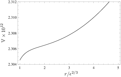
Two comments are in order: first, it is clear that exactly at the tip, i.e. $r=\epsilon^{2/3}$ the slow-roll parameter is simply $\varepsilon_{\mathrm{tip}}=0$. Second, away from the tip, $\varepsilon(r)$ can be reasonably small by choosing the parameters to allow for significant curvature perturbation spectrum at the end of inflation through the Lyth effect described in Section 3. In Fig. 1, we show the inflaton potential (5.22) and the slow-roll parameter $\varepsilon$ (5.26).

Figure 1: (Left) the inflaton potential (5.22) and (right) the slow-roll parameter $\varepsilon$ (5.26). We normalize $M_{\rm Pl}=1$ and for simplicity we set $A_{0}=1$. The point $r/\epsilon^{2/3}=1$ denotes the tip from which there is no further radial displacement. As shown in the right panel, the potential is very flat near the tip.

5.3 The angular stable trajectory and the degenerate residual isometry

In this section, we will argue that the angular stable trajectory near the tip region (5.12)-(5.14) for the Kuperstein embedding (5.7) is in fact valid along the entire deformed conifold by showing explicitly that the extremal values of the broken isometry directions along (5.12)-(5.14) are identical to the ones for the stable trajectory in the singular conifold (B.1), despite very different scalar potential in each region. Along this specific trajectory, we will then show that the proper distance associated with the residual isometry direction preserved by the Kuperstein embedding vanishes.

To begin with, we can rewrite the trajectory (5.12)-(5.14) in terms of the $\tau$ coordinate defined in (2.25) such that

$$z^{1}= -\epsilon\cosh\left(\frac{\tau}{2}\right)\,,$$ (5.32)

$$z^{2}= \pm i\epsilon\sinh\left(\frac{\tau}{2}\right)\,,$$ (5.33)

$$z^{3}= z^{4}=0\,.$$ (5.34)

Comparing the above with the deformed conifold coordinates (A.6)-(A.9), while one needs to solve transcendental equations in general, for sufficiently simple trajectory like (5.32)-(5.34), one can easily translate it in terms of the restriction on angular coordinates

$$+ : \theta_{1}=\theta_{2}=0\,,~~~\frac{\psi+(\phi_{1}+\phi_{2})}{2}=\pi\,,$$ (5.35)

$$- : \theta_{2}=\theta_{2}=\pi\,,~~~\frac{\psi-(\phi_{1}+\phi_{2})}{2}=0\,.$$ (5.36)

These two equivalent branches are the stabilized values of the isometry directions broken by the Kuperstein embedding (5.7). Exactly the same combinations of angles also appear when one compares the angular stable trajectory in the singular conifold (B.1) with the corresponding embedding coordinates written in terms of the angles. Since the embedding coordinates (A.6)-(A.9) interpolate the entire throat, and that the stabilized angular values are the same in both asymptotic regions, it is suggestive that the angular stable trajectory (5.12)-(5.14) is valid not only in the regions near or far away from the tip but also for the entire deformed conifold. It would be interesting to demonstrate this explicitly with the inflaton potential derived from the full warped deformed conifold metric.

One should note that on each branch, the dependence on the combination $[\psi\mp(\phi_{1}+\phi_{2})]/2$ vanishes from the scalar potential $V_{F}(z^{1}+\bar{z}^{1},|z^{1}|^{2},r,\sigma)$, despite the fact that $\psi$ and $(\phi_{1}+\phi_{2})/2$ appear individually in $z^{1}$ and $\bar{z}^{1}$. For each branch, the corresponding combination can take arbitrary value without affecting the resultant trajectory. Furthermore, it is also obvious that the combination $(\phi_{1}-\phi_{2})/2$ does not appear explicitly in $z^{1}$ or $\bar{z}^{1}$ hence in the scalar potential. Both $(\phi_{1}-\phi_{2})/2$ and one of $[\psi\mp(\phi_{1}+\phi_{2})]/2$ are the residual isometries preserved by the stable inflationary trajectory in the Kuperstein embedding (5.7).

The presence of the light additional residual isometries can in principle give significant contribution to the power spectrum by the Lyth effect we discussed in Section 3, by coupling them with the canonical inflaton through the tachyon potential at the end of the inflation. However the magnitude of such effect is also controlled by the stabilized values of broken isometry directions, and the dependence is encoded in the measure factors $\Gamma_{2}$ and $\Gamma_{3}$. We can easily calculate them by using (A.15)-(A.21) and writing out explicitly the metrics of $S^{2}$ and $S^{3}$ in terms of the deformed conifold angular coordinates as

$$d\Omega_{2}: ~\frac{(2/3)^{1/3}}{8}\left[(g_{1})^{2}+(g_{2})^{2}\right]\,,$$ (5.37)

$$d\Omega_{3}: ~\frac{(2/3)^{2/3}}{2}\left[(g_{3})^{2}+(g_{4})^{2}+\frac{1}{2}(g_{5})^{2}\right]\,.$$ (5.38)

Restricting them to the specific trajectories (5.35) and (5.36), we obtain

$$+ : ~d\Omega_{2}=0\,,~~~d\Omega_{3}=\frac{(2/3)^{2/3}}{2}\left\{d\left[\psi+(\phi_{1}+\phi_{2})\right]\right\}^{2}=0\,,$$ (5.39)

$$- : ~d\Omega_{2}=0\,,~~~d\Omega_{3}=\frac{(2/3)^{2/3}}{2}\left\{d\left[\psi-(\phi_{1}+\phi_{2})\right]\right\}^{2}=0\,.$$ (5.40)

Hence for both $(\phi_{1}-\phi_{2})/2$ and $[\psi\mp(\phi_{1}+\phi_{2})]/2$, their measure factors $\Gamma_{2}$ and $\Gamma_{3}$ vanish identically along (5.12)-(5.14), or equivalently (5.35) and (5.36). In other words, even though the $D3$-$\overline{D3}$ angular separations $\Delta[(\phi_{1}-\phi_{2})/2]$ and $\Delta\{[\psi\mp(\phi_{1}+\phi_{2})]/2\}$ can be finite, the proper separations along these directions in fact vanish. Therefore, despite having the necessary conditions, e.g. small slow-roll parameter $\varepsilon$ for the Lyth effect to be potentially significant, the calculations here demonstrate that, due to the degeneracy of the residual isometry directions, it in fact does not take place along the specific angular stable trajectory considered. However, for other embeddings that preserve some residual isometries on the $S^{3}$ at the tip of the conifold [31], our results in Section 3 can be used to estimate the size of these end of inflation effects. One can easily use for example the formula (3.13) to obtain the ratio between the power spectrum at the horizon exit and the end of inflation as

$$\frac{\mathcal{P}_{\zeta_{\rm e}}}{\mathcal{P}_{k}}=\frac{\varepsilon_{k}}{\varepsilon_{\rm e}}\frac{1}{2\left[(\vartheta_{\rm c}/\vartheta_{{\rm e}})^{2}-1\right]}\,.$$ (5.41)

The ratio $\varepsilon_{k}/\varepsilon_{\rm e}$ can be as large as ${\mathcal{O}}(1)$, while $(\theta_{c}/\theta_{\rm e})^{2}\gtrsim 1$, therefore in the scenario we described eariler, where Coulombic attraction is decoupled, $\mathcal{P}_{\zeta_{\rm e}}$ can possibly give comparable contribution to the power spectrum $\mathcal{P}_{k}$.

6 Discussion

In this paper, we studied the systematics of multi-field effects at the end of warped $D$ brane inflation. We discussed the necessary criteria for the isocurvature perturbations generated by the angular motion of a mobile $D3$ brane to be converted into the curvature perturbations usually associated with its radial motion in this scenario. We found that the significance of the end of inflation effects considered in Ref. [22] depends on the specific mechanism for uplifting the vacuum energy. If the uplifting is due to some distant $\overline{D3}$ branes or a $D$-term potential, the Coulombic potential can easily become subdominant even towards the end of inflation, and the effects described in Ref. [22] can in principle be significant. However, in the most explicit $D$ brane inflation constructed to date [12, 13], the $D7$ brane embedding chosen [24] does not yield such effects, regardless of the uplifting mechanism. This latter result is specific to the embedding of the moduli stabilizing branes as well as the infrared geometry of the throat. Along the stable trajectory for the embedding considered in Ref. [24], the proper distance for the residual isometry direction vanishes in the entire throat, the moduli space vanishes at the tip. It would be interesting to examine other $D7$ brane embeddings and/or other warped throats which leave a moduli space of vacua at the tip. Examples of such embeddings for the deformed conifold appeared in Ref. [31], where the residual isometry directions reside on the finite size $S^{3}$. However, finding an angular stable trajectory in these examples may remain challenging. Nevertheless, our results underscore the importance of multi-field effects in string inflation, as noted also in the context of DBI inflation recently in Ref. [54] (see also earlier discussions in Refs. [55, 56]).

As discussed in Section 3, the strength of the Lyth effect depends on the ratio $\varepsilon_{k}/\varepsilon_{e}$. Since the flat region of the inflaton potential considered in Refs. [12, 13] is an inflection point, $\varepsilon_{k}$ depends sensitively on where around the inflection point corresponds to the CMB scale. Given a $D$ brane inflation model which can yield the Lyth effect considered here, a precise determination of the amplitude of such effects would require the use of the full KS metric [37]. This is yet another context in which details of the warped geometries in the infrared can have significant effects on the CMB observations [57]. Furthermore, regardless of the Lyth effect studied here, a detailed comparison of the WMAP data with microscopic parameters of $D$ brane inflation requires identifying the relevant part of the inflaton potential which generates the observed CMB anisotropy, and the full KS metric is essential. Work along these lines is underway.

Finally, one may hope to also realize the curvaton mechanism [58] using these light fields. In the setup we discussed, however, inflation ends as $D3$ and $\overline{D3}$ annihilate and thus the would-be curvaton fields themselves disappear. For the same reason, any multi-field effect [59] after inflation will not be present as long as they are associated with $D3$ or $\overline{D3}$ branes. Nevertheless it would be interesting to implement the curvaton scenario in a different setup satisfying a number of constraints [60].

Acknowledgement

We are indebted to Bret Underwood for numerous valuable insights and discussions, and for collaboration at the initial stage of this project. We are also grateful to Misao Sasaki for discussions and comments on the manuscript. We thank Daniel Baumann, Chong-Sun Chu, Min-Xin Huang, David Lyth, Fernando Marchesano, Liam McAllister, Peter Ouyang, Sudhakar Panda, and Fernando Quevedo for helpful discussions. HYC would like to thank KITP at USCB and the Sixth Simons Workshop at SUNY Stony Brook for their hospitalities where part of the work was being carried out. JG is grateful to the Santa Fe 08 Cosmology Summer Workshop for hospitality where this work was being finished. The work of HYC and GS is supported in part by NSF Career Award No. PHY-0348093, DOE grant DE-FG-02-95ER40896, a Research Innovation Award and a Cottrell Scholar Award from Research Corporation, and a Vilas Associate Award from the University of Wisconsin. JG is partly supported by the Korea Research Foundation Grant KRF-2007-357-C00014 funded by the Korean Government.

Appendix A Details of the warped deformed conifold

Here we collect a few facts concerning the various coordinates parameterizing the deformed conifold. It is defined via the equation

$$\sum_{A=1}^{4}(z^{A})^{2}=\epsilon^{2}\,,$$ (A.1)

and the $D7$ brane embeddings we use are given in terms of one or the other of these sets of coordinates. These coordinates can be related to coordinates on the $S^{3}$ at the bottom of the throat as follows. We follow Ref. [61] with some modifications to their notation. We define the matrix $W$ as

$$W\equiv LW_{0}R^{\dagger}\,,$$ (A.2)

with

$$W_{0}\equiv\left(\begin{array}[]{cc}\epsilon/\sqrt{2}&\sqrt{r^{3}-\epsilon^{2}}\\ 0&-\epsilon/2\\ \end{array}\right)\,,$$ (A.3)

where $L$ and $R$ are $SU(2)$ matrices parameterized by three Euler angles (We are using the standard $r$-variable on the conifold, related to that in Ref. [61] by $r=r_{\mathrm{there}}^{2/3}$). We choose the convention

$$W=\begin{pmatrix}-w_{3}\;w_{2}\cr-w_{1}\;w_{4}\end{pmatrix}=-\frac{1}{\sqrt{2}}\begin{pmatrix}z^{3}+iz^{4}\;\;\;\;z^{1}-iz^{2}\cr z^{1}+iz^{2}\;\;-z^{3}+iz^{4}\end{pmatrix}\,,$$ (A.4)

where we have chosen the $w$’s so as to agree with (32)-(35) of Ref. [18] when we use the parameterization of Euler angles given in (2.24) and (2.25) of Ref. [61]. One indeed finds that

$${\rm det}\ W=w_{1}w_{2}-w_{3}w_{4}=-\frac{1}{2}\sum_{A=1}^{4}(z^{A})^{2}=-\frac{1}{2}\epsilon^{2}\,,$$ (A.5)

as required. At generic $r>\epsilon^{2/3}$, one of the six Euler angles in $L$ and $R$ is redundant, and the remaining five along with $r$ parameterize the deformed conifold. For $r\gg\epsilon^{2/3}$ the deformed conifold is well approximated by the singular conifold, with the angles parameterizing $T^{1,1}$.

The complex embedding coordinates of deformed conifold $\{z^{1},z^{2},z^{3},z^{4}\}$ can be expressed in terms of the real coordinates $\{\tau\in{\mathbb{R}\,,~\psi\in[0,4\pi]\,,~\theta_{1,2}\in[0,\pi]\,,~\phi_{1,2}\in[0,2\pi]}\}$, $\Xi=\tau+i\psi$ as

$$z^{1}= \epsilon\left[\cosh\left(\frac{\Xi}{2}\right)\cos\left(\frac{\theta_{1}+\theta_{2}}{2}\right)\cos\left(\frac{\phi_{1}+\phi_{2}}{2}\right)+i\sinh\left(\frac{\Xi}{2}\right)\cos\left(\frac{\theta_{1}-\theta_{2}}{2}\right)\sin\left(\frac{\phi_{1}+\phi_{2}}{2}\right)\right]\,,$$ (A.6)

$$z^{2}= \epsilon\left[-\cosh\left(\frac{\Xi}{2}\right)\cos\left(\frac{\theta_{1}+\theta_{2}}{2}\right)\sin\left(\frac{\phi_{1}+\phi_{2}}{2}\right)+i\sinh\left(\frac{\Xi}{2}\right)\cos\left(\frac{\theta_{1}-\theta_{2}}{2}\right)\cos\left(\frac{\phi_{1}+\phi_{2}}{2}\right)\right]\,,$$ (A.7)

$$z^{3}= \epsilon\left[-\cosh\left(\frac{\Xi}{2}\right)\sin\left(\frac{\theta_{1}+\theta_{2}}{2}\right)\cos\left(\frac{\phi_{1}-\phi_{2}}{2}\right)+i\sinh\left(\frac{\Xi}{2}\right)\sin\left(\frac{\theta_{1}-\theta_{2}}{2}\right)\sin\left(\frac{\phi_{1}-\phi_{2}}{2}\right)\right]\,,$$ (A.8)

$$z^{4}= \epsilon\left[-\cosh\left(\frac{\Xi}{2}\right)\sin\left(\frac{\theta_{1}+\theta_{2}}{2}\right)\sin\left(\frac{\phi_{1}-\phi_{2}}{2}\right)-i\sinh\left(\frac{\Xi}{2}\right)\sin\left(\frac{\theta_{1}-\theta_{2}}{2}\right)\cos\left(\frac{\phi_{1}-\phi_{2}}{2}\right)\right]\,.$$ (A.9)

At the tip of the throat $r=\epsilon^{2/3}$, we can reduce the complex coordinates $z^{A}$ in terms of the angles of the $S^{3}$ $\{\theta\,,\omega\,,\phi\}$ as

$$z^{1}= \epsilon\sin\left(\frac{\theta}{2}\right)\sin\left(\frac{\omega-\phi}{2}\right)\,,$$ (A.10)

$$z^{2}= \epsilon\sin\left(\frac{\theta}{2}\right)\cos\left(\frac{\omega-\phi}{2}\right)\,,$$ (A.11)

$$z^{3}= \epsilon\cos\left(\frac{\theta}{2}\right)\cos\left(\frac{\omega+\phi}{2}\right)\,,$$ (A.12)

$$z^{4}= \epsilon\cos\left(\frac{\theta}{2}\right)\sin\left(\frac{\omega+\phi}{2}\right)\,.$$ (A.13)

We see that in this case, $S^{3}$ is a real slice of each $z^{\alpha}$ coordinate and the metric is given by

$$d\Omega_{3}=(d\omega+\cos\theta d\phi)^{2}+d\theta^{2}+\sin^{2}\theta d\phi^{2}\,.$$ (A.14)

A.1 Metric

It is convenient to work in a diagonal basis of the metric by using the basis of one forms [37]

$$g^{1}\equiv \frac{e^{1}-e^{3}}{\sqrt{2}}\,,~~~g^{2}\equiv\frac{e^{2}-e^{4}}{\sqrt{2}}\,,$$

$$g^{3}\equiv \frac{e^{1}+e^{3}}{\sqrt{2}}\,,~~~g^{4}\equiv\frac{e^{2}+e^{4}}{\sqrt{2}}\,,$$

$$g^{5}\equiv e^{5}\,,$$ (A.15)

where

$$e^{1}\equiv -\sin\theta_{1}d\phi_{1}\,,$$ (A.16)

$$e^{2}\equiv d\theta_{1}\,,$$ (A.17)

$$e^{3}\equiv \cos\psi\sin\theta_{2}d\phi_{2}-\sin\psi d\theta_{2}\,,$$ (A.18)

$$e^{4}\equiv \sin\psi\sin\theta_{2}d\phi_{2}+\cos\psi d\theta_{2}\,,$$ (A.19)

$$e^{5}\equiv d\psi+\cos\theta_{1}d\phi_{1}+\cos\theta_{2}d\phi_{2}\,.$$ (A.20)

The metric of the deformed conifold is then

$$ds_{6}^{2}=\frac{1}{2}\epsilon^{4/3}K(\tau)\left\{\frac{1}{3[K(\tau)]^{3}}[d\tau^{2}+(g^{5})^{2}]+\cosh^{2}\left(\frac{\tau}{2}\right)\left[(g^{3})^{2}+(g^{4})^{2}\right]+\sinh^{2}\left(\frac{\tau}{2}\right)\left[(g^{1})^{2}+(g^{2})^{2}\right]\right\}\,,$$ (A.21)

where

$$K(\tau)=\frac{\left[\sinh(2\tau)-2\tau\right]^{1/3}}{2^{1/3}\sinh\tau}\,.$$ (A.22)

The ten dimensional metric takes the warped form

$$ds_{10}^{2}=e^{2A(y)}\eta_{\mu\nu}dx^{\mu}dx^{\nu}+e^{-2A(y)}ds_{6}^{2}\,,$$ (A.23)

where the warp factor is given by the expression [37]

$$e^{4A(\tau)}=2^{2/3}(g_{s}M\alpha^{\prime})^{2}\epsilon^{-8/3}I(\tau)\,,$$ (A.24)

where

$$I(\tau)\equiv\int_{\tau}^{\infty}dx\ \frac{x\coth x-1}{\sinh^{2}x}\left[\sinh(2x)-2x\right]^{1/3}\,.$$ (A.25)

A.2 Little Kähler potential

The warped deformed conifold metric (A.21) can be obtained from the “little” Kähler potential $k(z^{\alpha},\bar{z}^{\bar{\beta}})$ as

$$\tilde{g}_{\alpha\bar{\beta}}=\partial_{\alpha}\partial_{\bar{\beta}}k\,.$$ (A.26)

Because the angular directions of the warped deformed conifold are isometries they do not appear explicitly in the little Kähler potential, and in general the Kähler potential only depends on the radial coordinate $\tau$ through [61]

$$k(\tau)=\frac{\epsilon^{4/3}}{2^{1/3}}\int_{0}^{\tau}d\tau^{\prime}\left[\sinh(2\tau^{\prime})-2\tau^{\prime}\right]^{1/3}\,,$$ (A.27)

where without loss of generality we set the integration constant to zero. Using the relation between $\tau$ and $r$, we can approximately solve for the large and small $r$ limits as

$$k(r)\to\left\{\begin{split}&\frac{3}{2}r^{2}&\mbox{for }&r\gg\epsilon^{2/3}\,,\\ &k_{0}+\frac{c}{\epsilon^{2/3}}(r^{3}-\epsilon^{2})&\mbox{for }&r\approx\epsilon^{2/3}\,,\end{split}\right.$$ (A.28)

where $c=2^{1/6}/3^{1/3}\approx 1.61887$.

Appendix B Brief review of the “Delicate Universe”

In Refs. [12, 13], the authors considered the region of large $D3$-$\overline{D3}$ separation, so that the deformed conifold can be approximated by its singular limit. The expression for the $F$-term potential (2.14) is then greatly simplified. The non-perturbative superpotential is generated by $D3$ or $D7$ brane wrapping a four cycle of the conifold (made compact by the bulk geometry). Further, their presence partially breaks the full $SO(4)$ isometry group of the deformed conifold. For example, consider the simplest Kuperstein embedding given by holomorphic function (5.7) which breaks $SO(4)$ down to an $SO(3)$ subgroup rotating $\{z^{2},z^{3},z^{4}\}$. The trajectory of the canonical inflaton then further breaks it to $SO(2)$. One should note here that in the presence of the bulk NS-NS B-field, the $D7$ brane embedding (5.7) can remain supersymmetric without additional worldvolume flux: by contrast, the supersymmetric $D7$ embeddings considered in the singular conifold limit as given in Refs. [62, 63, 64] can only remain supersymmetric on these four cycles in the deformed conifold with additional worldvolume flux turned on [65].

Using the singular conifold metric and (5.7) to calculate $V_{F}$, the authors then included the Coulombic potential $V_{D3\overline{D3}}$ as given by (4.5) such that the cancellation of the negative vacuum energy of $V_{F}$ is due to the combination of the $\overline{D3}$ branes at the tip of the deformed conifold and distant bulk. They stabilize the isometry directions broken by $D7$ branes, and the resulting angular stable trajectory is given by

$$z^{1}=-\frac{r^{3/2}}{\sqrt{2}}\leftrightarrow\frac{\partial(V_{F}+V_{D3\overline{D3}})}{\partial\Psi_{i}}=0\,.$$ (B.1)

Here $\{\Psi_{i}\}$ runs through the broken isometry directions and (B.1) also imposes constraints on other embedding coordinates $z^{2}=\pm iz^{1}\,,~z^{3}=z^{4}=0$. The axion $\varsigma$ can also be stabilized by tuning the perturbative superpotential $W_{0}$ to be negative. To proceed obtaining single field inflation, an adiabatic approximation is taken to stabilize the volume modulus $\sigma$ by solving the equation

$$\left.\frac{\partial(V_{F}+V_{D3\overline{D3}})(r,\sigma)}{\partial\sigma}\right|_{\sigma_{\ast}}=0\,.$$ (B.2)

The authors approximated the solution of (B.2) by

$$\sigma_{\ast}(r)\approx\sigma_{0}\left[1+c_{3/2}\frac{r^{2}}{(2\mu^{2})^{2/3}}\right]\,,$$ (B.3)

where $\mu$ is the embedding parameter in (5.7) and the coefficient $c_{3/2}\approx[1-1/(2a\sigma_{F})]/(n\sigma_{F})$, and $\sigma_{0}$ is the stabilized volume at the tip of the throat after including the uplifting term $V_{D3\overline{D3}}$. Finally, the canonical inflaton $\phi$ was related to the radial coordinate of the mobile $D3$ brane via (2.29).

Putting everything together, the single inflaton potential derived at large brane separation for the trajectory (B.1) is subsequently given by

$${\mathbb{V}}({\phi_{r}})= \frac{\kappa^{2}a|A_{0}|^{2}e^{-2a\sigma_{\ast}}}{3[U({\phi_{r}},\sigma_{\star})]^{2}}h({\phi_{r}})^{2/n}\left\{2a\sigma_{\ast}+6-6e^{a\sigma_{\ast}}\frac{|W_{0}|}{|A_{0}|}h({\phi_{r}})^{1/n}+\frac{3}{nh({\phi_{r}})}\frac{{\phi_{r}}}{\phi_{\mu}}\left[c_{0}-h({\phi_{r}})\sqrt{\frac{{\phi_{r}}}{\phi_{\mu}}}\right]\right\}$$

$$+\frac{D_{0}+D_{\rm others}}{[U({\phi_{r}},\sigma_{\ast})]^{2}}\,,$$ (B.4)

where

$$h({\phi_{r}})= 1+\left(\frac{{\phi_{r}}}{\phi_{\mu}}\right)^{3/2}\,,$$ (B.5)

$$c_{0}= \frac{9}{4na\sigma_{0}\phi_{\mu}^{2}/M_{\rm Pl}^{2}}\,,$$ (B.6)

$$\phi_{\mu}^{2}= \frac{3}{2}T_{3}(2\mu^{2})^{2/3}\,.$$ (B.7)

Here the approximation $D({\phi_{r}})\approx D_{0}+D_{\rm others}$ is taken for large radius $r\gg\epsilon^{2/3}$. The explicit inflaton potential (B.4) represents one of the most well developed and top-down brane inflation model to date, which explicitly includes the effects of compactification and moduli stabilization. To obtain sufficiently flat region of ${\mathbb{V}}(\phi)$, the parameters in the inflaton potential need to be ‘delicately’ tuned. For the specific set of parameters considered in Ref. [13] (see below Fig. 2 there), the inflaton potential ${\mathbb{V}}(\phi)$ has a sharp drop, however it is induced by the $D3$-$\overline{D3}$ Coulombic interaction which only becomes significant near the tip of the throat, without which the inflaton potential is in fact smooth and inflation continues until much smaller radius into the deformed conifold. However in such region, the singular conifold approximation should break down. In Fig. 2 we show the effective potential (B.4) and the related slow-roll parameters.

Figure 2: (Upper left) the inflaton potential (B.4) and the resulting slow-roll parameters, (upper right) $\varepsilon$ and (lower left) $\eta$. We show both cases where the Coulombic piece proportional to $r^{-4}$ is present (solid line) and absent (dotted line). As can be seen, without the Coulombic term inflation proceeds deep inside the throat, i.e. very small $r$ region, but (B.4) is no more valid there. In the lower right panel, we show $-\dot{H}/H^{2}$ which is exactly equivalent to the acceleration of the scale factor: $-\dot{H}/H^{2}<1$ means acceleration. Clearly, the criteria $|\eta|=1$ does not guarantee that inflation ends at the corresponding point, especially when the Coulombic term is negligible which is the scenario we discussed in the main text.

Of course, it is possible that one can try to select a different set of parameters such that the slow-roll parameters $\varepsilon$ and $\eta$ become order one at much larger radius without including the Coulombic interaction. The point we would like to emphasize is that for the purpose of parameter scanning, consistently excluding the tip region in the analysis of inflation imposes further constraints (in addition to obtaining a sufficient number of $e$-folds, and the correct amplitude of the power spectrum, etc). However if we relax such constraints and allow the inflationary epoch to extend deep into the deformed conifold region, one needs to take into account the full deformed conifold metric. As we have explicitly shown in the main text, $\varepsilon$ can remain small in this region, using the metric near the tip of deformed conifold. In other words, inflation ends when the canonical inflaton reaches its limit in field range, rather than when $\varepsilon$ becomes large. In such case, there can potentially be an additional contribution to the curvature perturbation arising from quantum fluctuations in the light residual isometry directions, which can significantly modify the estimates made far from the tip.

In relation to the scenario we proposed in the main text, where $V_{\rm Coulomb}$ is neglected, the potential (B.4) should be regarded as the ultraviolet completion of our inflaton potential (5.22) with uplifting exclusively done by distant $\overline{D3}$ branes. Assuming that the flat region in (B.4) (near its inflection point) corresponds to the large observable scales, and that most but not all the $e$-folds are generated there, this allows us to have an estimate of $\varepsilon_{k}$ near the horizon exit. To make such statement precise of course requires the calculation of the inflaton potential with respect to the full deformed conifold metric, this is an interesting although potentially challenging direction, which we shall return in the near future.

Appendix C Stability analysis for angular extremum trajectory

In this appendix we will explicitly obtain the angular extremum trajectory for the Kuperstein embedding (5.7) in the near tip region of deformed conifold, and demonstrate its stability.

First, without lost of generality, we take both $\mu$ and $\epsilon$ to be real, and let us write the $F$-term scalar potential $V_{F}=V_{\mathrm{KKLT}}+\Delta V_{F}$ in the following form:

$$V_{\mathrm{KKLT}}= \frac{2a\kappa^{2}|A_{0}|^{2}e^{-2a\sigma}}{[U(r,\sigma)]^{2}}\left|1-\frac{z_{1}}{\mu}\right|^{2/n}\left\{1-e^{a\sigma}\frac{|W_{0}|}{|A_{0}|}\left|1-\frac{z_{1}}{\mu}\right|^{-1/n}+\frac{a}{6}\left[2\sigma-\gamma k_{0}+\gamma c\epsilon^{4/3}\left(1-\frac{{\epsilon^{2}}}{r^{3}}\right)\right]\right\}$$

$$= \mathcal{A}(r,\sigma)\left(1-\frac{z_{1}+\bar{z}_{1}}{\mu}+\frac{|z_{1}|^{2}}{\mu^{2}}\right)^{1/n}\left\{1-e^{a\sigma}\frac{|W_{0}|}{|A_{0}|}\left(1-\frac{z_{1}+\bar{z}_{1}}{\mu}+\frac{|z_{1}|^{2}}{\mu^{2}}\right)^{-1/(2n)}+\mathcal{B}(r,\sigma)\right\}\,,$$ (C.1)

and

$$\Delta{V}_{F}= \frac{\kappa^{2}|A_{0}|^{2}e^{-2a\sigma}}{3n^{2}[U(r,\sigma)]^{2}}\left|1-\frac{z_{1}}{\mu}\right|^{2(1/n-1)}\left\{\frac{\epsilon^{2/3}}{c\mu^{2}\gamma}\left(1-\frac{|z_{1}|^{2}}{r^{3}}\right)+\frac{an}{\mu}\left[\left(1-\frac{\bar{z}_{1}}{\mu}\right)\left(z_{1}-\bar{z}_{1}\frac{\epsilon^{2}}{r^{3}}\right)+c.c.\right]\right\}$$

$$= \mathcal{C}(r,\sigma)\left(1-\frac{z_{1}+\bar{z}_{1}}{\mu}+\frac{|z_{1}|^{2}}{\mu^{2}}\right)^{1/n-1}$$

$$\times\left\{\frac{\epsilon^{2/3}}{c\mu^{2}\gamma}\left(1-\frac{|z_{1}|^{2}}{r^{3}}\right)+an\left[\frac{z_{1}+\bar{z}_{1}}{\mu}\left(1-\frac{\epsilon^{2}}{r^{3}}\right)+\frac{(z_{1}+\bar{z}_{1})^{2}}{\mu^{2}}\frac{\epsilon^{2}}{r^{3}}-\frac{2|z_{1}|^{2}}{\mu^{2}}\left(1+\frac{\epsilon^{2}}{r^{3}}\right)\right]\right\}\,.$$ (C.2)

Such explicit forms (C.1) and (C.2) will be useful in the subsequent stability analysis. Note that both $\mathcal{A}$ and $\mathcal{C}$ have mass dimension 4 and the remaining terms are dimensionless, and we have rewritten the expressions in terms of $|z_{1}|^{2}$ and $z_{1}+\bar{z}_{1}$ wherever possible. From (C.1) and (C.2), $V_{F}$ now becomes a function of $\sigma$, $r$, $z_{1}+\bar{z}_{1}$ and $|z_{1}|^{2}$. To extract the light degree of freedom among all the isometry directions, we first try to stabilize as many angular directions explicitly broken by the presence of $D7$ as possible.

Recalling the analysis of Ref. [13], where the trajectory in the singular conifold along which the linear variations of $|z_{1}|^{2}$ and $z_{1}+\bar{z}_{1}$ vanish, we can again apply this analysis and write down the variation of $z_{1}$ being

$$\delta z_{1}^{(0)}=\sum_{j=2}^{4}\alpha_{j}z^{(0)}_{j}\ ,$$ (C.3)

with $\alpha_{i}\in{\mathbb{R}}$. Here $\left\{z^{(0)}_{1},z^{(0)}_{2},z^{(0)}_{3},z^{(0)}_{4}\right\}$ are the coordinates of a fiducial point and from here ${\alpha_{2},\alpha_{3},\alpha_{4},\beta_{3},\beta_{4}}\subset\{\Psi_{i}\}$ are local coordinates on the base of the cone. Vanishing of the linear variations can then be written as

$$\delta|z_{1}|^{2}= \sum^{4}_{j=2}\alpha_{j}\left[z^{(0)}_{1}\bar{z}^{(0)}_{j}+\bar{z}^{(0)}_{1}z^{(0)}_{j}\right]=0\,,$$ (C.4)

$$\delta(z_{1}+\bar{z}_{1})= i\sum_{j=2}^{4}\alpha_{j}\left[z^{(0)}_{j}-\bar{z}_{j}^{(0)}\right]=0\,.$$ (C.5)

For (C.4) to be satisfied for all $\{\alpha_{i}\}$, we need to have

$$z_{j}^{(0)}=i\varrho_{j}z_{1}^{(0)}\,,$$ (C.6)

where $\varrho_{j}\in\mathbb{R}$. Using the $SO(3)$ symmetry, one can set $\varrho_{2}\neq 0$ while $\varrho_{3}=\varrho_{4}=0$. (C.5) then implies $z_{1}^{(0)}$ is strictly real. Subjecting $z^{(0)}_{1}$ and $z^{(0)}_{2}$ to the constraint $\left(z_{1}^{(0)}\right)^{2}+\left(z_{2}^{(0)}\right)^{2}=\epsilon^{2}$ and the definition $r^{3}=|z_{1}|^{2}+|z_{2}|^{2}=\left(z_{1}^{(0)}\right)^{2}+\left|z_{2}^{(0)}\right|^{2}$, we can see that

$$\varrho_{2}=\pm\sqrt{\frac{r^{3}-\epsilon^{2}}{r^{3}+\epsilon^{2}}}\,,$$ (C.7)

leading to the angular extremum trajectory along

$$z_{1}^{(0)}= \pm\sqrt{\frac{r^{3}+\epsilon^{2}}{2}}\,,$$ (C.8)

$$z_{2}^{(0)}= \pm i\sqrt{\frac{r^{3}-\epsilon^{2}}{2}}\,.$$ (C.9)

Notice that in the singular conifold limit $\epsilon\to 0$, (C.8) and (C.9) reduce to the one in (B.1).

Let us now proceed with the stability analysis for (C.8) and (C.9). We first notice that along these trajectories the linear perturbations in $|z_{1}|^{2}$ and $z_{1}+\bar{z}_{1}$ disappear, and we can further see that

$$z_{1}= z_{1}^{(0)}\left[1-\frac{1}{2}\left(\alpha_{2}^{2}+\alpha_{3}^{2}+\alpha_{3}^{2}\right)+\frac{i}{2}\varrho_{2}\left(2\alpha_{2}-\alpha_{3}\beta_{3}-\alpha_{4}\beta_{4}\right)+\cdots\right]\,,$$ (C.10)

$$z_{1}+\bar{z}_{1}= 2z_{1}^{(0)}\left[1-\frac{1}{2}\left(\alpha_{2}^{2}+\alpha_{3}^{2}+\alpha_{3}^{2}\right)+\cdots\right]\,,$$ (C.11)

$$|z_{1}|^{2}= {z_{1}^{(0)}}^{2}\left[1-\left(\frac{2\epsilon^{2}}{r^{3}+\epsilon^{2}}\alpha_{2}^{2}+\alpha_{3}^{2}+\alpha_{4}^{2}\right)+\cdots\right]\,.$$ (C.12)

Then we find that

$$\left.\frac{\partial^{2}|z_{1}|^{2}}{\partial\Psi_{i}\partial\Psi_{j}}\right|_{0}= -(r^{3}+\epsilon^{2})\left(\frac{2\epsilon^{2}}{r^{3}+\epsilon^{2}}\delta_{i2}\delta_{j2}+\delta_{i3}\delta_{j3}+\delta_{i4}\delta_{j4}\right)\,,$$ (C.13)

$$\left.\frac{\partial^{2}(z_{1}+\bar{z}_{1})}{\partial\Psi_{i}\partial\Psi_{j}}\right|_{0}= \mp\sqrt{2(r^{3}+\epsilon^{2})}(\delta_{i2}\delta_{j2}+\delta_{i3}\delta_{j3}+\delta_{i4}\delta_{j4})\,,$$ (C.14)

so that the mass matrix along the extremal trajectory is given by

$$\left.\frac{\partial^{2}V}{\partial\Psi_{i}\partial\Psi_{j}}\right|_{0}=\left(\begin{array}[]{ccccc}X+2\epsilon^{2}Y/(r^{3}+\epsilon^{2})&0&0&0&0\\ 0&X+Y&0&0&0\\ 0&0&X+Y&0&0\\ 0&0&0&0&0\\ 0&0&0&0&0\\ \end{array}\right)\,,$$ (C.15)

where

$$X= \mp\sqrt{2(r^{3}+\epsilon^{2})}\left.\frac{\partial{V}}{\partial(z_{1}+\bar{z}_{1})}\right|_{0}\,,$$ (C.16)

$$Y= -(r^{3}+\epsilon^{2})\left.\frac{\partial{V}}{\partial|z_{1}|^{2}}\right|_{0}\,.$$ (C.17)

Therefore, three angular directions, viz. $\alpha_{2}$, $\alpha_{3}$ and $\alpha_{4}$ have definite masses squared no matter positive or negative, while $\beta_{3}$ and $\beta_{4}$ remain perfectly flat unless any other effect which breaks the symmetry is introduced, e.g. bulk mass terms. Hence, if we are to look for light angular directions which can give rise to interesting and/or dangerous effects at the end of inflation, there are two of them provided that the other three directions are stabilized. First we must check whether this is indeed achieved.

From (C.1) and (C.2), after some calculations, we can find that for $V_{\mathrm{KKLT}}$

$$\left.\frac{\partial{V_{\mathrm{KKLT}}}}{\partial(z_{1}+\bar{z}_{1})}\right|_{0}= -\frac{\mathcal{A}}{n\mu}\left|1\mp\frac{\sqrt{r^{3}+\epsilon^{2}}}{\sqrt{2}\mu}\right|^{-2(1-1/n)}\left(1-\frac{e^{a\sigma}}{2}\frac{|W_{0}|}{|A_{0}|}\left|1\mp\frac{\sqrt{r^{3}+\epsilon^{2}}}{\sqrt{2}\mu}\right|^{-1/n}+\mathcal{B}\right)\,,$$ (C.18)

$$\left.\frac{\partial{V_{\mathrm{KKLT}}}}{\partial|z_{1}|^{2}}\right|_{0}= \frac{\mathcal{A}}{n\mu^{2}}\left|1\mp\frac{\sqrt{r^{3}+\epsilon^{2}}}{\sqrt{2}\mu}\right|^{-2(1-1/n)}\left(1-\frac{e^{a\sigma}}{2}\frac{|W_{0}|}{|A_{0}|}\left|1\mp\frac{\sqrt{r^{3}+\epsilon^{2}}}{\sqrt{2}\mu}\right|^{-1/n}+\mathcal{B}\right)\,,$$ (C.19)

and for $\Delta{V}_{F}$

$$\left.\frac{\partial\Delta{V}_{F}}{\partial(z_{1}+\bar{z}_{1})}\right|_{0}= \frac{\mathcal{C}}{\mu}\left|1\mp\frac{\sqrt{r^{3}+\epsilon^{2}}}{\sqrt{2}\mu}\right|^{-2(2-1/n)}$$

$$\times\left\{\left(1-\frac{1}{n}\right)\left[\frac{\epsilon^{2/3}}{c\mu^{2}\gamma}\frac{r^{3}-\epsilon^{2}}{2r^{3}}-an\left(1-\frac{\varepsilon^{2}}{r^{3}}\right)\frac{\sqrt{2(r^{3}+\varepsilon^{2})}}{\mu}\left(\frac{\sqrt{r^{3}+\epsilon^{2}}}{\sqrt{2}\mu}\mp 1\right)\right]\right.$$

$$\hskip 14.22636pt\left.+an\left|1\mp\frac{\sqrt{r^{3}+\epsilon^{2}}}{\sqrt{2}\mu}\right|^{2}\left[\left(1-\frac{\epsilon^{2}}{r^{3}}\right)\pm\frac{2\sqrt{2(r^{3}+\epsilon^{2})}}{\mu}\frac{\epsilon^{2}}{r^{3}}\right]\right\}\,,$$ (C.20)

$$\left.\frac{\partial\Delta{V}_{F}}{\partial|z_{1}|^{2}}\right|_{0}= -\frac{\mathcal{C}}{\mu^{2}}\left|1\mp\frac{\sqrt{r^{3}+\epsilon^{2}}}{\sqrt{2}\mu}\right|^{-2(2-1/n)}$$

$$\times\left\{\left(1-\frac{1}{n}\right)\left[\frac{\epsilon^{2/3}}{c\mu^{2}\gamma}\frac{r^{3}-\epsilon^{2}}{2r^{3}}-an\left(1-\frac{\epsilon^{2}}{r^{3}}\right)\frac{\sqrt{2(r^{3}+\epsilon^{2})}}{\mu}\left(\frac{\sqrt{r^{3}+\epsilon^{2}}}{\sqrt{2}\mu}\mp 1\right)\right]\right.$$

$$\left.\hskip 14.22636pt+\left|1\mp\frac{\sqrt{r^{3}+\epsilon^{2}}}{\sqrt{2}\mu}\right|^{2}\left[\frac{\epsilon^{2/3}}{cr^{3}\gamma}+2an\left(1+\frac{\epsilon^{2}}{r^{3}}\right)\right]\right\}\,.$$ (C.21)

Thus, from

$$\mathcal{C}=\frac{\mathcal{A}}{6an^{2}}\,,$$ (C.22)

we can write

$$X= \pm\frac{\mathcal{A}}{n}\frac{\sqrt{2(r^{3}+\epsilon^{2})}}{\mu}\left|1\mp\frac{\sqrt{r^{3}+\epsilon^{2}}}{\sqrt{2}\mu}\right|^{-2(1-1/n)}$$

$$\times\left\{1-\frac{e^{a\sigma}}{2}\frac{|W_{0}|}{|A_{0}|}\left|1\mp\frac{\sqrt{r^{3}+\epsilon^{2}}}{\sqrt{2}\mu}\right|^{-1/n}+\mathcal{B}-\frac{1}{6}\left[\left(1-\frac{\epsilon^{2}}{r^{3}}\right)\pm\frac{2\sqrt{2(r^{3}+\epsilon^{2})}}{\mu}\frac{\epsilon^{2}}{r^{3}}\right]\right.$$

$$\left.\hskip 22.76228pt-\frac{1-1/n}{6}\left[\frac{\epsilon^{2/3}}{anc\mu^{2}\gamma}\frac{r^{3}-\epsilon^{2}}{2r^{3}}-\left(1-\frac{\epsilon^{2}}{r^{3}}\right)\frac{\sqrt{2(r^{3}+\epsilon^{2})}}{\mu}\left(\frac{\sqrt{r^{3}+\epsilon^{2}}}{\sqrt{2}\mu}\mp 1\right)\right]\right\}$$ (C.23)

$$Y= -\frac{\mathcal{A}}{n}\frac{r^{3}+\epsilon^{2}}{\mu^{2}}\left|1\mp\frac{\sqrt{r^{3}+\epsilon^{2}}}{\sqrt{2}\mu}\right|^{-2(1-1/n)}$$

$$\times\left\{1-\frac{e^{a\sigma}}{2}\frac{|W_{0}|}{|A_{0}|}\left|1\mp\frac{\sqrt{r^{3}+\epsilon^{2}}}{\sqrt{2}\mu}\right|^{-1/n}+\mathcal{B}-\frac{1}{6}\left[\frac{\epsilon^{2/3}}{ancr^{3}\gamma}+2\left(1+\frac{\epsilon^{2}}{r^{3}}\right)\right]\right.$$

$$\left.\hskip 22.76228pt-\frac{1-1/n}{6}\left[\frac{\epsilon^{2/3}}{anc\mu^{2}\gamma}\frac{r^{3}-\epsilon^{2}}{2r^{3}}-\left(1-\frac{\epsilon^{2}}{r^{3}}\right)\frac{\sqrt{2(r^{3}+\epsilon^{2})}}{\mu}\left(\frac{\sqrt{r^{3}+\epsilon^{2}}}{\sqrt{2}\mu}\mp 1\right)\right]\right\}\,.$$ (C.24)

Note that we can write $Y$ using $X$ as

$$Y=\mp\frac{\sqrt{r^{3}+\epsilon^{2}}}{\sqrt{2}\mu}X+\frac{\mathcal{A}}{6n\mu^{2}}(r^{3}+\epsilon^{2})\left|1\mp\frac{\sqrt{r^{3}+\epsilon^{2}}}{\sqrt{2}\mu}\right|^{-2(1-1/n)}\left\{1+\frac{\epsilon^{2/3}}{ancr^{3}\gamma}+\left[3\mp\frac{2\sqrt{2(r^{3}+\epsilon^{2})}}{\mu}\right]\frac{\epsilon^{2}}{r^{3}}\right\}\,.$$ (C.25)

To estimate the stability near the tip, let us take the limit $r^{3}\to\epsilon^{2}$, i.e. very close to the end of the inflationary epoch. Then, from (C.23) and (C.24), we can see that

$$X\to \pm\frac{2\mathcal{A}}{n}\frac{\epsilon}{\mu}\left|1\mp\frac{\epsilon}{\mu}\right|^{-2(1-1/n)}\left[1-\frac{e^{a\sigma}}{2}\frac{|W_{0}|}{|A_{0}|}\left|1\mp\frac{\epsilon}{\mu}\right|^{-1/n}+\frac{a}{6}(2\sigma-\gamma k_{0})\mp\frac{2\epsilon}{3\mu}\right]\,,$$ (C.26)

$$Y\to -\frac{2\mathcal{A}}{n}\left(\frac{\epsilon}{\mu}\right)^{2}\left|1\mp\frac{\varepsilon}{\mu}\right|^{-2(1-1/n)}\left[\frac{1}{3}-\frac{e^{a\sigma}}{2}\frac{|W_{0}|}{|A_{0}|}\left|1\mp\frac{\epsilon}{\mu}\right|^{-1/n}+\frac{a}{6}(2\sigma-\gamma k_{0})-\frac{1}{6anc\epsilon^{4/3}\gamma}\right]$$

$$=\mp\frac{\epsilon}{\mu}X+\frac{\mathcal{A}}{3n}\left(\frac{\epsilon}{\mu}\right)^{2}\left|1\mp\frac{\epsilon}{\mu}\right|^{-2(1-1/n)}\left[4\left(1\mp\frac{\epsilon}{\mu}\right)+\frac{1}{anc\epsilon^{4/3}\gamma}\right]\,.$$ (C.27)

Further, in this limit, all the eigenvalues in (C.15) become $X+Y$, so that for the angular stability along $\alpha_{2}$, $\alpha_{3}$ and $\alpha_{4}$ we require that

$$X+Y=\left(1\mp\frac{\epsilon}{\mu}\right)X+\frac{\mathcal{A}}{3n}\left(\frac{\epsilon}{\mu}\right)^{2}\left|1\mp\frac{\epsilon}{\mu}\right|^{-2(1-1/n)}\left[4\left(1\mp\frac{\epsilon}{\mu}\right)+\frac{1}{anc\epsilon^{4/3}\gamma}\right]>0\,.$$ (C.28)

To complete the analysis we therefore need extra information, e.g. the value of the stabilized volume modulus at the tip $\sigma_{0}$ and the ratio $\epsilon/\mu$. Since $\epsilon/\mu$ is the ratio of the size of the tip $\epsilon$ to the distance of the stack of $D7$ branes to the tip $\mu$, one can easily tune it such that $\epsilon/\mu<1$. Therefore it is sufficient to check the positivity of (C.26). For this, we apply the results we establish in the following appendix (D.4) and (D.9) related to $\sigma_{0}$: then the terms in the square brackets of (C.26) can be written as

$$1-\frac{e^{a\sigma}}{2}\frac{|W_{0}|}{|A_{0}|}\left|1\mp\frac{\epsilon}{\mu}\right|^{-1/n}+\frac{a}{6}(2\sigma-\gamma k_{0})\mp\frac{2\epsilon}{3\mu}\approx\frac{1}{2}-\frac{bs}{6}\mp\frac{2\epsilon}{3\mu}\approx\frac{1}{2}-\frac{bs}{6}\,.$$ (C.29)

Thus the angular stability depends on the product $bs$: if $bs>3$ we obtain negative sign while $bs<3$ it becomes positive. Since we know that the power $b$ for our uplifting potential is either 2 (for $V_{D3\overline{D3}}$) or 3 (for $V_{D\mathrm{-term}}$) and that $1<s\lesssim\mathcal{O}(3)$, the product $bs$ lies in the range

$$2<bs\lesssim\mathcal{O}(9)\,.$$ (C.30)

We can therefore see that the condition for angular stability $bs>3$ can be naturally satisfied. Thus we conclude that $z_{1}^{(0)}=-\sqrt{(r^{3}+\varepsilon^{2})/2}$ is the stable trajectory we have been searching for very near the tip.

Appendix D Derivation of approximated stabilized volume

Having derived the angular stable trajectory $z_{1}=-\sqrt{(r^{3}+\epsilon^{2})/2}$, we are left with a two-field potential $V_{F}(r,\sigma)=V_{\mathrm{KKLT}}(r,\sigma)+\Delta V_{F}(r,\sigma)$. In this appendix we will derive an approximate expression of the stabilized volume $\sigma_{\star}(r)$ in term of the radial coordinate $r$ that is given by (5.19).

D.1 Stabilized volume at the tip

Without taking into account of the uplifting term and the additional contribution from the $D3$ brane position, we have the usual anti de Sitter minimum of KKLT compactification, the stabilized volume modulus $\sigma_{F}$ is defined to be

$$\left.\frac{\partial{V}_{F}}{\partial\sigma}(r,\sigma)\right|_{r=\epsilon^{2/3},\sigma=\sigma_{F}}=0\,.$$ (D.1)

Explicitly $\sigma_{F}$ can be given by the transcendental equation

$$\frac{|W_{0}|}{|A_{0}|}e^{a\sigma_{F}}{\mathcal{G}}^{1/n}=1+\frac{aU_{F}}{3}\,,$$ (D.2)

where ${\mathcal{G}}$ is defined by (5.29) and

$$U_{F}=2\sigma_{F}-\gamma k_{0}\,.$$ (D.3)

Thus at the tip, the potential is given by

$$V_{F}(r=\varepsilon^{2/3},\sigma=\sigma_{F})=\left.V_{\rm KKLT}\right|_{r=\epsilon^{2/3}}=-\frac{a^{2}\kappa^{2}|A_{0}|^{2}e^{-2a\sigma_{F}}}{3U_{F}}{\mathcal{G}}^{-2/n}\,.$$ (D.4)

Notice that $\Delta V_{F}$ vanishes at $r=\epsilon^{2/3}$.

Now consider including the effect of uplifting term $V_{D}(r,\sigma)$ which we assume to take the form in (4.5). We expect such a term contributes a small shift to the stabilized volume at the tip of the throat $\sigma_{0}=\sigma_{F}+\delta\sigma$, which is formally defined as

$$\left.\frac{\partial{(V_{F}+V_{D})}}{\partial\sigma}\right|_{r=\varepsilon^{2/3},\sigma=\sigma_{0}}\approx\left.\frac{\partial^{2}V_{F}}{\partial\sigma^{2}}\right|_{\sigma_{F}}\delta\sigma+\left.\frac{\partial{V_{D}}}{\partial\sigma}\right|_{\sigma_{0}}=0\,,$$ (D.5)

where

$$\left.\frac{\partial V_{D}}{\partial\sigma}\right|_{\sigma_{0}}= -\frac{2bV_{D}}{2\sigma_{0}-\gamma k_{0}}\approx-\frac{bV_{D}}{\sigma_{F}}\left[1-(b+1)\left(\frac{\delta\sigma}{\sigma_{F}}+\frac{\gamma k_{0}}{2\sigma_{F}}\right)\right]\,.$$ (D.6)

Solving (D.5) and (D.6), we obtain

$$\frac{\delta\sigma}{\sigma_{F}}\approx\left[1-(b+1)\frac{\gamma k_{0}}{2\sigma_{F}}\right]\left[(b+1)+\left.\frac{\sigma_{F}^{2}}{bV_{D}}\frac{\partial^{2}V_{F}}{\partial\sigma^{2}}\right|_{\sigma_{F}}\right]^{-1}\,.$$ (D.7)

We can also find that

$$\left.\frac{\partial^{2}V_{F}}{\partial\sigma^{2}}\right|_{r=\varepsilon^{2/3},\sigma=\sigma_{F}}= \frac{2a\kappa^{2}|A_{0}|^{2}e^{-2a\sigma_{F}}}{U_{F}^{2}}{\mathcal{G}}^{-2/n}\left(\frac{a^{3}U_{F}}{3}+\frac{5}{3}a^{2}-\frac{16a}{3U_{F}}\right)$$

$$\approx 2a^{2}\frac{a^{2}\kappa^{2}|A_{0}|^{2}e^{-2a\sigma_{F}}}{3U_{F}}{\mathcal{G}}^{-2/n}$$

$$= 2a^{2}|V_{F}(r=\epsilon^{2/3},\sigma=\sigma_{F})|\,,$$ (D.8)

where we have used the fact that typically $\sigma_{F}\gg 1$. The shift of the stabilized volume can then be approximated as

$$\delta\sigma\approx\frac{bs}{2a^{2}\sigma_{F}}\,,$$ (D.9)

where the parameter $s$ is the uplifting ratio given by (4.9).

D.2 Radial dependence

Now let us also take into account the dependence of the stabilized volume on the brane position, denoted as $\sigma_{\star}(r)$. Formally this amounts to solving the equation

$$\left.\frac{\partial[V_{F}(r,\sigma)+V_{D}(r,\sigma)]}{\partial\sigma}\right|_{\sigma_{\star}(r)}=0\,.$$ (D.10)

From (5.15), (5.16) and (4.5) and the previous analysis, the volume modulus $\sigma$ appears in both the exponential and the polynomial, (D.10) is thus in fact a transcendental equation. To simplify the analysis, one notices that in the large $\sigma_{F}/\sigma_{0}$ limit, one can approximate $\sigma_{\star}(r)$ in the polynomial by $\sigma_{0}$ [13], as the difference is exponentially suppressed. Then we are left with a quadratic equation of $X\equiv\exp(-a\sigma_{\star})$ given by

$$A_{2}X^{2}+A_{1}X-A_{0}=0\,,$$ (D.11)

so that

$$\sigma_{\star}=\frac{1}{a}\log\left[\frac{2A_{2}}{A_{1}}\left(-1-\sqrt{1+\frac{4A_{0}A_{2}}{A_{1}^{2}}}\right)^{-1}\right]\,.$$ (D.12)

Two comments are in order: first, we note that

$$A_{0}=\frac{2bD(|\mathbf{y}-\mathbf{\bar{y}}|)}{U_{\sigma_{0}}^{b+1}}\propto\frac{1}{\sigma_{0}^{b+1}}\,,$$ (D.13)

with $b=2$ or 3. Therefore, unless we care for corrections beyond $\mathcal{O}(1/\sigma_{0}^{b+1})$, the factor $4A_{0}A_{2}/A_{1}^{2}$ in the square root does not alter the leading contribution if there exist terms up to $\mathcal{O}(1/\sigma_{0}^{b})$, which is indeed the case as will be shown. Second, since we are interested in the region very close to $r=\epsilon^{2/3}$, the primary expansion parameter will be $r-\epsilon^{2/3}$ which we denote by $x$ below. Thus we expect

$$\frac{2A_{2}}{A_{1}}\left(-1-\sqrt{1+\frac{4A_{0}A_{2}}{A_{1}^{2}}}\right)^{-1}= -\frac{A_{2}}{A_{1}}+\mathcal{O}\left(\frac{1}{\sigma_{0}^{b+1}}\right)$$

$$= e^{a\sigma_{F}}\left\{\left[\mathcal{O}(1)+\mathcal{O}\left(\frac{1}{\sigma_{0}}\right)+\cdots+\mathcal{O}\left(\frac{1}{\sigma_{0}^{b}}\right)\right]\right.$$

$$\left.\hskip 28.45274pt+\left[\mathcal{O}(1)+\mathcal{O}\left(\frac{1}{\sigma_{0}}\right)+\cdots+\mathcal{O}\left(\frac{1}{\sigma_{0}^{b}}\right)\right]x+\cdots\right\}\,.$$ (D.14)

After some calculations, we can find that schematically

$$-\frac{A_{2}}{A_{1}}=e^{a\sigma_{F}}\left(c_{0}+c_{1}x\right)\,,$$ (D.15)

where the coefficients are given such that

$$c_{0}= 1+\mathcal{O}\left(\frac{1}{\sigma_{F}^{2}}\right)\,,$$ (D.16)

$$c_{1}= \mp\frac{3\epsilon^{1/3}}{4n\mu}\left|1\pm\frac{\epsilon}{\mu}\right|^{-1}+\mathcal{O}\left(\frac{1}{\sigma_{F}}\right)\,,$$ (D.17)

so that

$$\sigma_{\star}\approx\sigma_{F}\left(1+\frac{c_{1}}{a\sigma_{F}}x\right)\,.$$ (D.18)

One notices that in contrast with Ref. [13], where the leading radial dependence enters at order $r^{3/2}$, here with the deformation parameter $\epsilon\neq 0$, we only have a rational expansion. Furthermore as $\sigma_{F}$ and $\sigma_{0}$ only differs at order $1/\sigma_{F}$, we can replace $\sigma_{F}$ by $\sigma_{0}$ in (D.18).

Appendix E Calculations of the slow-roll parameter

In this section we present explicit calculation of the slow-roll parameter $\varepsilon$ given in the main text. From (2.8), (5.19), (5.20) and (A.28), the derivatives of $\sigma_{\star}(r)$ and $U[r,\sigma_{\star}(r)]$ with respect to the radial coordinate $r$ are given by

$$\frac{\partial\sigma_{\star}(r)}{\partial{r}}= \frac{3\epsilon^{1/3}}{4an\mu}{\mathcal{G}}\,,$$ (E.1)

$$\frac{\partial U[r,\sigma_{\star}(r)]}{\partial{r}}= \frac{3\epsilon^{1/3}}{2an\mu}{\mathcal{G}}-\frac{3c\gamma}{\epsilon^{2/3}}r^{2}\,,$$ (E.2)

respectively, where ${\mathcal{G}}$ is again given by (5.29). Given these, now let us calculate the derivatives of $\mathbb{V}$ with respect to $r$ from (5.23), (5.24) and (5.25). For notational simplicity, from below let us denote

$$g(r)\equiv 1+\frac{\sqrt{r^{3}+\epsilon^{2}}}{\sqrt{2}\mu}\,.$$ (E.3)

We can find, after some simple calculations, that the first derivatives with respect to $r$ are given by

$$\frac{\partial{V_{\mathrm{KKLT}}}}{\partial{r}}= V_{\mathrm{KKLT}}\left\{-\frac{3\epsilon^{1/3}}{n\mu}\mathcal{G}\left(\frac{1}{2}+\frac{1}{aU}\right)+\frac{6c\gamma}{\epsilon^{2/3}U}r^{2}+\frac{3r^{2}}{2n\mu^{2}[g(r)-1]g(r)}\right\}$$

$$+\frac{2\kappa^{2}a|A_{0}|^{2}e^{-2a\sigma_{\star}}}{U^{2}}\left[g(r)\right]^{2/n}$$

$$\hskip 14.22636pt\times\left\{\frac{|W_{0}|}{|A_{0}|}e^{a\sigma_{\star}}\left[g(r)\right]^{-1/n}\left[-\frac{3\epsilon^{1/3}}{4n\mu}\mathcal{G}+\frac{3r^{2}}{4n\mu^{2}[g(r)-1]g(r)}\right]+\frac{a}{2}\left[\frac{\epsilon^{1/3}}{2an\mu}\mathcal{G}+c\gamma\frac{\epsilon^{10/3}}{r^{4}}\right]\right\}\,,$$ (E.4)

$$\frac{\partial\Delta{V_{F}}}{\partial{r}}= \Delta{V_{F}}\left\{-\frac{3\epsilon^{1/3}}{n\mu}\mathcal{G}\left(\frac{1}{2}+\frac{1}{aU}\right)+\frac{6c\gamma}{\epsilon^{2/3}U}r^{2}+\left(\frac{1}{n}-1\right)\frac{3r^{2}}{2\mu^{2}[g(r)-1]g(r)}\right\}$$

$$+\frac{\kappa^{2}|A_{0}|^{2}e^{-2a\sigma_{\star}}}{n^{2}U^{2}}\left[g(r)\right]^{2(1/n-1)}$$

$$\hskip 14.22636pt\times\left\{\left(1-\frac{\epsilon^{2}}{r^{3}}\right)\frac{(an-1)g(r)+1}{g(r)-1}\frac{r^{2}}{2\mu^{2}}+\frac{\epsilon^{2}}{r^{4}}\left[\frac{\epsilon^{2/3}}{2c\mu^{2}\gamma}-2an[g(r)-1]g(r)\right]\right\}\,,$$ (E.5)

$$\frac{\partial{V_{D}}}{\partial{r}}= \frac{1}{U^{b}}\left\{\frac{\partial{D(|\mathbf{y}-\mathbf{\bar{y}}|)}}{\partial{r}}-\frac{bD(|\mathbf{y}-\mathbf{\bar{y}}|)}{U}\left[\frac{3\epsilon^{1/3}}{2an\mu}\mathcal{G}-\frac{3c\gamma}{\epsilon^{2/3}}r^{2}\right]\right\}\,.$$ (E.6)

As can be read from the above expressions, in general $\varepsilon$ is a complex functions of $r$. To catch a clearer feeling, it would be useful to evaluate them at the tip, i.e. at $r=\epsilon^{2/3}$. (E.4), (E.5) and (E.6) then become

$$\left.\frac{\partial{V_{\mathrm{KKLT}}}}{\partial{r}}\right|_{r=\epsilon^{2/3}}= \left|V_{\mathrm{KKLT}}|_{r=\epsilon^{2/3}}\right|\frac{3}{U_{F}}\left[\frac{3\epsilon^{1/3}}{2an\mu}{\mathcal{G}}-c\gamma\epsilon^{2/3}\right]\,,$$ (E.7)

$$\left.\frac{\partial\Delta{V_{F}}}{\partial{r}}\right|_{r=\epsilon^{2/3}}= \left|V_{\mathrm{KKLT}}|_{r=\epsilon^{2/3}}\right|\frac{3}{a^{2}n^{2}U_{F}}{\mathcal{G}}^{2}\left[\frac{\epsilon^{2/3}}{2c\mu^{2}\gamma}-2an\frac{\epsilon}{\mu}{\mathcal{G}}^{-1}\right]\epsilon^{-2/3}\,,$$ (E.8)

$$\left.\frac{\partial{V_{D}}}{\partial{r}}\right|_{r=\epsilon^{2/3}}= \frac{1}{U_{F}^{b}}\left\{\left.\frac{\partial{D}}{\partial{r}}\right|_{r=\epsilon^{2/3}}-\frac{bD|_{r=\epsilon^{2/3}}}{U_{F}}\left[\frac{3\epsilon^{1/3}}{2an\mu}{\mathcal{G}}-3c\gamma\epsilon^{2/3}\right]\right\}\,,$$ (E.9)

where $V_{\mathrm{KKLT}}|_{r=\epsilon^{2/3}}$ is given by (D.4) and $U_{F}$ by (D.3). Hence, we have

$$\left.\frac{\partial{{\mathbb{V}}}}{\partial{r}}\right|_{r=\epsilon^{2/3}}= \frac{3\left|V_{\mathrm{KKLT}}|_{r=\epsilon^{2/3}}\right|}{U_{F}}\left\{\left[\frac{3\epsilon^{1/3}}{2an\mu}{\mathcal{G}}-c\gamma\epsilon^{2/3}\right]\right.\left.+\frac{{\mathcal{G}}^{2}}{a^{2}n^{2}\epsilon^{2/3}}\left[\frac{\epsilon^{2/3}}{2c\mu^{2}\gamma}-2an\frac{\epsilon}{\mu}{\mathcal{G}}^{-1}\right]\right\}$$

$$+\frac{1}{U_{F}^{b}}\left\{\left.\frac{\partial{D}}{\partial{r}}\right|_{r=\epsilon^{2/3}}-\frac{bD|_{r=\epsilon^{2/3}}}{U_{F}}\left[\frac{3\epsilon^{1/3}}{2an\mu}{\mathcal{G}}-3c\gamma\epsilon^{2/3}\right]\right\}\,.$$ (E.10)

Further, from (4.9) we can relate $V_{D}|_{r=\epsilon^{2/3}}$ with $V_{\mathrm{KKLT}}|_{r=\epsilon^{2/3}}$ by

$$V_{D}|_{r=\epsilon^{2/3}}=\frac{D|_{r=\epsilon^{2/3}}}{U_{F}^{b}}=s|V_{\mathrm{KKLT}}|_{r=\epsilon^{2/3}}|\,.$$ (E.11)

This further simplifies (E.10) into

$$\left.\frac{\partial{{\mathbb{V}}}}{\partial{r}}\right|_{r=\epsilon^{2/3}}= |V_{\mathrm{KKLT}}|_{r=\epsilon^{2/3}}|\left\{\frac{3-sb}{U_{F}}\left[\frac{3\epsilon^{1/3}}{4\pi\mu}{\mathcal{G}}-c\gamma\epsilon^{2/3}\right]+\frac{2sbc\gamma}{U_{F}}\epsilon^{2/3}+\frac{s}{D}\left.\frac{\partial{D}}{\partial{r}}\right|_{r=\epsilon^{2/3}}\right.$$

$$\hskip 71.13188pt\left.+\frac{3{\mathcal{G}}^{2}}{4\pi^{2}U_{F}}\left[\frac{\epsilon^{2/3}}{2c\mu^{2}\gamma}-4\pi\frac{\epsilon}{\mu}{\mathcal{G}}^{-1}\right]\epsilon^{2/3}\right\}\,.$$ (E.12)

Likewise, using the fact that $\Delta{V_{F}}|_{r=\epsilon^{2/3}}=0$,

$${\mathbb{V}}|_{r=\epsilon^{2/3}}= V_{\mathrm{KKLT}}|_{r=\epsilon^{2/3}}+\Delta{V_{F}}|_{r=\epsilon^{2/3}}+V_{D}|_{r=\epsilon^{2/3}}$$

$$= V_{\mathrm{KKLT}}|_{r=\epsilon^{2/3}}+V_{D}|_{r=\epsilon^{2/3}}$$

$$= (s-1)|V_{\mathrm{KKLT}}|_{r=\epsilon^{2/3}}|\,.$$ (E.13)

Thus, at the tip we obtain

$$\left.\frac{\partial{{\mathbb{V}}}/\partial{r}}{{\mathbb{V}}}\right|_{r=\epsilon^{2/3}}= \frac{1}{s-1}\left\{\frac{3-sb}{U_{F}}\left[\frac{3\epsilon^{1/3}}{4\pi\mu}{\mathcal{G}}-c\gamma\epsilon^{2/3}\right]+\frac{2sbc\gamma}{U_{F}}\epsilon^{2/3}+\frac{s}{D}\left.\frac{\partial{D}}{\partial{r}}\right|_{r=\epsilon^{2/3}}\right.$$

$$\hskip 34.14322pt\left.+\frac{3{\mathcal{G}}^{2}}{4\pi^{2}U_{F}}\left[\frac{\epsilon^{2/3}}{2c\mu^{2}\gamma}-4\pi\frac{\epsilon}{\mu}{\mathcal{G}}^{-1}\right]\epsilon^{2/3}\right\}\,.$$ (E.14)

Note that $D$ contains the factor $|\mathbf{y}-\mathbf{\bar{y}}|$ and that its derivative is given by

$$\frac{\partial|\mathbf{y}-\mathbf{\bar{y}}|}{\partial{r}}=2(r-\epsilon^{2/3})\,,$$ (E.15)

we can easily see that the term involving $\partial{D(|\mathbf{y}-\mathbf{\bar{y}}|)}/\partial{r}$ in fact vanishes at $r=\epsilon^{2/3}$ for $V_{D3\overline{D3}}$ with $b=2$, whereas for $V_{D\mathrm{-term}}$ with $b=3$ such term vanishes identically as $D(|\mathbf{y}-\mathbf{\bar{y}}|)=v_{D}$. In other words, $\varepsilon_{\rm end}$ for the two different uplifting mechanisms only differ in $b$. The canonically normalized inflaton near the tip is identified as in (2.31) and $\partial_{\phi_{\tau}}=(\partial r/\partial{\phi_{\tau}})\partial_{r}$. Note that $\epsilon$ and $\mu$, $\gamma$, and $r$ have mass dimension of –3/2, 2 and –1 respectively, so it can be easily seen that $(\partial{{\mathbb{V}}}/\partial{r})/{\mathbb{V}}$ has mass dimension 1 by counting the dimensionful parameters.

Since (E.14) is clearly finite, from the chain rule (5.27) one can easily see that the slow-roll parameter $\varepsilon$ in fact vanishes identically at the tip $r=\epsilon^{2/3}$, or ${\phi_{\tau}}=0$. However we can expand around the tip and obtain the lowest order approximation as

$$\varepsilon(r)\approx\left.\frac{M_{\rm Pl}^{2}}{3T_{3}\epsilon^{4/3}}\left(\frac{\partial{{\mathbb{V}}}/\partial{r}}{{\mathbb{V}}}\right)^{2}\right|_{r=\epsilon^{2/3}}\left(r^{2}-\epsilon^{4/3}\right)\,,$$ (E.16)

with $(\partial{{\mathbb{V}}}/\partial{r})/{\mathbb{V}}|_{r=\epsilon^{2/3}}$ given by (E.14). We can express $\varepsilon(r)$ in terms of the compactification parameters describing the bulk and throat geometries [13]. Several useful expressions are

$$\frac{\hat{r}_{\mathrm{UV}}}{\epsilon^{2/3}}= \sqrt{\frac{3}{2}}\frac{r_{\mathrm{UV}}}{\epsilon^{2/3}}=\exp\left(\frac{2\pi K}{3g_{s}M}\right)\equiv a_{0}^{-1}\,,$$ (E.17)

$$Q_{\mu}\equiv \frac{r_{\mathrm{UV}}}{r_{\mu}}=\frac{r_{\mathrm{UV}}}{(2\mu^{2})^{1/3}}=\frac{2^{1/6}}{3^{1/2}a_{0}}\left(\frac{\epsilon}{\mu}\right)^{2/3}\,,$$ (E.18)

$$\gamma\approx \frac{B_{4}}{B_{6}}\frac{2\log{Q_{\mu}}}{3\pi r_{\mathrm{UV}}^{2}}=\frac{B_{4}}{B_{6}}\frac{2\log{Q_{\mu}}}{3\pi(2\mu^{2})^{2/3}Q_{\mu}^{2}}\,,$$ (E.19)

$$M_{\rm Pl}^{2}= \frac{T_{3}^{2}}{\pi}V_{6}^{w}=\frac{3}{8}NB_{6}T_{3}(2\mu^{2})^{2/3}Q_{\mu}^{2}\,,$$ (E.20)

$$U_{F}\approx 2\sigma_{F}\approx\frac{3N}{2\pi}B_{4}\log{Q_{\mu}}\,.$$ (E.21)

Here $\hat{r}_{\mathrm{UV}}$ denotes the ultraviolet cutoff radius where the deformed conifold is attached to the bulk Calabi-Yau, $r_{\mu}$ is the minimal radius of $D7$, and $B_{4}$ and $B_{6}$ denote the contributions of the throat to the warped volume of the wrapped four cycle and to the total warped volume of the compact space $V_{6}^{w}$, respectively. Substituting these into (E.14) and (E.16) and after a little calculations, we find

$$\left.\frac{\partial{{\mathbb{V}}}/\partial{r}}{{\mathbb{V}}}\right|_{r=\epsilon^{2/3}}= \frac{\mu^{-2/3}}{s-1}\left\{\frac{3-sb}{3NB_{4}\log{Q_{\mu}}}\left[\frac{3}{2}3^{1/12}\left(\frac{a_{0}Q_{\mu}}{c}\right)^{1/2}\left(1+3^{1/4}\left(\frac{a_{0}Q_{\mu}}{c}\right)^{3/2}\right)\right.\right.$$

$$\left.\hskip 113.81102pt-\frac{B_{4}}{B_{6}}\frac{2\cdot 2^{1/3}c\log{Q_{\mu}}}{3Q_{\mu}^{2}}3^{1/12}\left(\frac{a_{0}Q_{\mu}}{c}\right)\right]+\frac{4\cdot 2^{1/3}sbc}{9NB_{6}Q_{\mu}^{2}}3^{1/6}\left(\frac{a_{0}Q_{\mu}}{c}\right)$$

$$\hskip 34.14322pt+\frac{2}{NB_{4}\log{Q_{\mu}}}\left[1+3^{1/4}\left(\frac{a_{0}Q_{\mu}}{c}\right)^{3/2}\right]^{-2}$$

$$\left.\hskip 42.67912pt\times\left[\frac{B_{6}}{B_{4}}\frac{3Q_{\mu}^{2}}{8\cdot 2^{1/3}c\log{Q_{\mu}}}-3^{1/12}\left(\frac{a_{0}Q_{\mu}}{c}\right)^{1/2}\left(1+3^{1/4}\left(\frac{a_{0}Q_{\mu}}{c}\right)^{3/2}\right)\right]\right\}\,.$$ (E.22)

We can also observe from above that for the two different uplifting mechanisms, the value of $\varepsilon(r)$ only differ in $b$.

References

- [1] A. H. Guth, Phys. Rev. D 23, 347 (1981). A. D. Linde, Phys. Lett. B 108, 389 (1982) ; A. Albrecht and P. J. Steinhardt, Phys. Rev. Lett. 48, 1220 (1982).
- [2] See, e.g. A. R. Liddle and D. H. Lyth, “Cosmological inflation and large-scale structure,” Cambridge, UK: Univ. Pr. (2000) 400 p ; V. Mukhanov, “Physical foundations of cosmology,” Cambridge, UK: Univ. Pr. (2005) 421 p ; S. Weinberg, “Cosmology,” Oxford, UK: Univ. Pr. (2008)
- [3] D. H. Lyth and A. Riotto, Phys. Rept. 314, 1 (1999) [arXiv:hep-ph/9807278].
- [4] D. N. Spergel et al. [WMAP Collaboration], Astrophys. J. Suppl. 170, 335 (2007) [arXiv:astro-ph/0603449] ; M. Tegmark et al. [SDSS Collaboration], Phys. Rev. D 74, 123507 (2006) [arXiv:astro-ph/0608632] ; [SDSS Collaboration], Astrophys. J. Suppl. 172, 634 (2007) [arXiv:0707.3380 [astro-ph]] ; E. Komatsu et al. [WMAP Collaboration], arXiv:0803.0547 [astro-ph].
- [5] J. E. Lidsey, A. R. Liddle, E. W. Kolb, E. J. Copeland, T. Barreiro and M. Abney, Rev. Mod. Phys. 69, 373 (1997) [arXiv:astro-ph/9508078] ; S. Habib, K. Heitmann and G. Jungman, Phys. Rev. Lett. 94, 061303 (2005) [arXiv:astro-ph/0409599] ; M. Joy, E. D. Stewart, J. O. Gong and H. C. Lee, JCAP 0504, 012 (2005) [arXiv:astro-ph/0501659].
- [6] G. R. Dvali and S. H. H. Tye, Phys. Lett. B 450, 72 (1999) [arXiv:hep-ph/9812483].
- [7] G. R. Dvali, Q. Shafi and S. Solganik, arXiv:hep-th/0105203.
- [8] C. P. Burgess, M. Majumdar, D. Nolte, F. Quevedo, G. Rajesh and R. J. Zhang, JHEP 0107, 047 (2001) [arXiv:hep-th/0105204].
- [9] A. Linde, eConf C040802, L024 (2004) [J. Phys. Conf. Ser. 24, 151 (2005 PTPSA,163,295-322.2006)] [arXiv:hep-th/0503195]; S. H. Henry Tye, Lect. Notes Phys. 737, 949 (2008) [arXiv:hep-th/0610221]. J. M. Cline, arXiv:hep-th/0612129; R. Kallosh, Lect. Notes Phys. 738, 119 (2008) [arXiv:hep-th/0702059]. C. P. Burgess, PoS P2GC, 008 (2006) [Class. Quant. Grav. 24, S795 (2007)] [arXiv:0708.2865 [hep-th]]. L. McAllister and E. Silverstein, Gen. Rel. Grav. 40, 565 (2008) [arXiv:0710.2951 [hep-th]].
- [10] S. Kachru, R. Kallosh, A. Linde, J. M. Maldacena, L. P. McAllister and S. P. Trivedi, JCAP 0310, 013 (2003) [arXiv:hep-th/0308055].
- [11] E. J. Copeland, A. R. Liddle, D. H. Lyth, E. D. Stewart and D. Wands, Phys. Rev. D 49, 6410 (1994) [arXiv:astro-ph/9401011].
- [12] D. Baumann, A. Dymarsky, I. R. Klebanov, L. McAllister and P. J. Steinhardt, Phys. Rev. Lett. 99, 141601 (2007) [arXiv:0705.3837 [hep-th]].
- [13] D. Baumann, A. Dymarsky, I. R. Klebanov and L. McAllister, JCAP 0801, 024 (2008) [arXiv:0706.0360 [hep-th]].
- [14] S. Panda, M. Sami and S. Tsujikawa, Phys. Rev. D 76, 103512 (2007) [arXiv:0707.2848 [hep-th]].
- [15] C. P. Burgess, J. M. Cline, K. Dasgupta and H. Firouzjahi, JHEP 0703 (2007) 027 [arXiv:hep-th/0610320].
- [16] A. Krause and E. Pajer, arXiv:0705.4682 [hep-th].
- [17] E. Pajer, JCAP 0804 (2008) 031 [arXiv:0802.2916 [hep-th]].
- [18] D. Baumann, A. Dymarsky, I. R. Klebanov, J. M. Maldacena, L. P. McAllister and A. Murugan, JHEP 0611 (2006) 031 [arXiv:hep-th/0607050].
- [19] O. J. Ganor, Nucl. Phys. B 499, 55 (1997) [arXiv:hep-th/9612077].
- [20] M. Berg, M. Haack and B. Kors, Phys. Rev. D 71, 026005 (2005) [arXiv:hep-th/0404087].
- [21] S. Kachru, R. Kallosh, A. Linde and S. P. Trivedi, Phys. Rev. D 68 (2003) 046005 [arXiv:hep-th/0301240].
- [22] D. H. Lyth, JCAP 0511 (2005) 006 [arXiv:astro-ph/0510443]; L. Alabidi and D. Lyth, JCAP 0608, 006 (2006) [arXiv:astro-ph/0604569].
- [23] D. H. Lyth and A. Riotto, Phys. Rev. Lett. 97 (2006) 121301 [arXiv:astro-ph/0607326].
- [24] S. Kuperstein, JHEP 0503 (2005) 014 [arXiv:hep-th/0411097].
- [25] S. B. Giddings, S. Kachru and J. Polchinski, Phys. Rev. D 66, 106006 (2002) [arXiv:hep-th/0105097].
- [26] K. Dasgupta, G. Rajesh and S. Sethi, JHEP 9908, 023 (1999) [arXiv:hep-th/9908088].
- [27] H. L. Verlinde, Nucl. Phys. B 580, 264 (2000) [arXiv:hep-th/9906182].
- [28] B. R. Greene, K. Schalm and G. Shiu, Nucl. Phys. B 584, 480 (2000) [arXiv:hep-th/0004103].
- [29] S. Gukov, C. Vafa and E. Witten, Nucl. Phys. B 584, 69 (2000) [Erratum-ibid. B 608, 477 (2001)] [arXiv:hep-th/9906070].
- [30] O. DeWolfe and S. B. Giddings, Phys. Rev. D 67, 066008 (2003) [arXiv:hep-th/0208123].
- [31] O. DeWolfe, L. McAllister, G. Shiu and B. Underwood, JHEP 0709 (2007) 121 [arXiv:hep-th/0703088].
- [32] S. B. Giddings and A. Maharana, Phys. Rev. D 73, 126003 (2006) [arXiv:hep-th/0507158].
- [33] A. R. Frey and A. Maharana, JHEP 0608, 021 (2006) [arXiv:hep-th/0603233].
- [34] C. P. Burgess, P. G. Camara, S. P. de Alwis, S. B. Giddings, A. Maharana, F. Quevedo and K. Suruliz, JHEP 0804, 053 (2008) [arXiv:hep-th/0610255].
- [35] G. Shiu, G. Torroba, B. Underwood and M. R. Douglas, JHEP 0806, 024 (2008) [arXiv:0803.3068 [hep-th]].
- [36] M. R. Douglas and G. Torroba, arXiv:0805.3700 [hep-th].
- [37] I. R. Klebanov, M. J. Strassler, JHEP 0008, 052 (2000) [arXiv:hep-th/0007191].
- [38] S. Sarangi and S. H. H. Tye, Phys. Lett. B 573 (2003) 181 [arXiv:hep-th/0307078].
- [39] C. M. Brown and O. DeWolfe, arXiv:0806.4399 [hep-th].
- [40] O. Aharony, Y. E. Antebi and M. Berkooz, Phys. Rev. D 72 (2005) 106009 [arXiv:hep-th/0508080].
- [41] A. Ceresole, G. Dall’Agata, R. D’Auria and S. Ferrara, Phys. Rev. D 61, 066001 (2000) [arXiv:hep-th/9905226].
- [42] A. Ceresole, G. Dall’Agata and R. D’Auria, JHEP 9911, 009 (1999) [arXiv:hep-th/9907216].
- [43] O. DeWolfe, S. Kachru and H. L. Verlinde, JHEP 0405 (2004) 017 [arXiv:hep-th/0403123].
- [44] L. Leblond and S. Shandera, JCAP 0701, 009 (2007) [arXiv:hep-th/0610321].
- [45] A. A. Starobinsky, JETP Lett. 42 (1985) 152 [Pisma Zh. Eksp. Teor. Fiz. 42 (1985) 124] ; M. Sasaki and E. D. Stewart, Prog. Theor. Phys. 95, 71 (1996) [arXiv:astro-ph/9507001] ; J. O. Gong and E. D. Stewart, Phys. Lett. B 538, 213 (2002) [arXiv:astro-ph/0202098] ; D. H. Lyth, K. A. Malik and M. Sasaki, JCAP 0505, 004 (2005) [arXiv:astro-ph/0411220].
- [46] E. Komatsu and D. N. Spergel, Phys. Rev. D 63, 063002 (2001) [arXiv:astro-ph/0005036].
- [47] M. Sasaki, arXiv:0805.0974 [astro-ph] ; A. Naruko and M. Sasaki, arXiv:0807.0180 [astro-ph].
- [48] C. P. Burgess, R. Kallosh and F. Quevedo, JHEP 0310 (2003) 056 [arXiv:hep-th/0309187].
- [49] H. Jockers and J. Louis, Nucl. Phys. B 718, 203 (2005) [arXiv:hep-th/0502059].
- [50] D. Cremades, M. P. Garcia del Moral, F. Quevedo and K. Suruliz, JHEP 0705 (2007) 100 [arXiv:hep-th/0701154].
- [51] G. Villadoro and F. Zwirner, Phys. Rev. Lett. 95 (2005) 231602 [arXiv:hep-th/0508167].
- [52] K. Choi, A. Falkowski, H. P. Nilles and M. Olechowski, Nucl. Phys. B 718 (2005) 113 [arXiv:hep-th/0503216].
- [53] M. Haack, D. Krefl, D. Lust, A. Van Proeyen and M. Zagermann, JHEP 0701 (2007) 078 [arXiv:hep-th/0609211].
- [54] D. Langlois, S. Renaux-Petel, D. A. Steer and T. Tanaka, arXiv:0804.3139 [hep-th]; D. Langlois, S. Renaux-Petel, D. A. Steer and T. Tanaka, arXiv:0806.0336 [hep-th].
- [55] M. x. Huang, G. Shiu and B. Underwood, Phys. Rev. D 77, 023511 (2008) [arXiv:0709.3299 [hep-th]].
- [56] D. A. Easson, R. Gregory, D. F. Mota, G. Tasinato and I. Zavala, JCAP 0802, 010 (2008) [arXiv:0709.2666 [hep-th]].
- [57] G. Shiu and B. Underwood, Phys. Rev. Lett. 98, 051301 (2007) [arXiv:hep-th/0610151]; S. Kecskemeti, J. Maiden, G. Shiu and B. Underwood, JHEP 0609, 076 (2006) [arXiv:hep-th/0605189].
- [58] A. D. Linde and V. F. Mukhanov, Phys. Rev. D 56, 535 (1997) [arXiv:astro-ph/9610219] ; D. H. Lyth and D. Wands, Phys. Lett. B 524, 5 (2002) [arXiv:hep-ph/0110002] ; T. Moroi and T. Takahashi, Phys. Lett. B 522, 215 (2001) [Erratum-ibid. B 539, 303 (2002)] [arXiv:hep-ph/0110096].
- [59] J. O. Gong, Phys. Rev. D 75, 043502 (2007) [arXiv:hep-th/0611293] ; K. Y. Choi and J. O. Gong, JCAP 0706, 007 (2007) [arXiv:0704.2939 [astro-ph]] ; J. O. Gong, Phys. Lett. B 657, 165 (2007) [arXiv:0706.3599 [astro-ph]].
- [60] J. O. Gong, Phys. Lett. B 637, 149 (2006) [arXiv:hep-ph/0602106].
- [61] P. Candelas and X. C. de la Ossa, Nucl. Phys. B 342, 246 (1990);
- [62] P. Ouyang, Nucl. Phys. B 699 (2004) 207 [arXiv:hep-th/0311084].
- [63] A. Karch and E. Katz, JHEP 0206 (2002) 043 [arXiv:hep-th/0205236].
- [64] D. Arean, D. E. Crooks and A. V. Ramallo, JHEP 0411 (2004) 035 [arXiv:hep-th/0408210].
- [65] H. Y. Chen, P. Ouyang, and G. Shiu, in preparation
- [66] J. O. Gong and E. D. Stewart, Phys. Lett. B 510, 1 (2001) [arXiv:astro-ph/0101225].