Infinite sequences of fixed point free pseudo-Anosov homeomorphisms.

Abstract. We construct infinite sequences of pseudo-Anosov homeomorphisms without fixed points and leaving invariant a sequence of orientable measured foliations on the same topological surface and the same stratum of the space of abelian differentials. The existence of such sequences shows that all pseudo-Anosov homeomorphisms fixing orientable measured foliations cannot be obtained by the Rauzy induction strategy.

2000 Mathematics Subject Classification. Primary: 37E30. ÊSecondary: 32G15, 57R30, 37B10
Key words and phrases. Pseudo Anosov homeomorphisms, Rauzy induction, fixed points, train-track maps

1 Introduction

This work started after a discussion between ÊA.Avila and P.Hubert. The question was : ”Is there a pseudo-Anosov homeomorphism fixing an orientable measured foliation and without fixed points of negative index?”

It turns out that one such example already existed in the litterature due to P.Arnoux and J.C.Yoccoz, [A.Y], [A]. It was constructed for a very different purpose and no general technics was available to build other examples.

Existence or non existence of fixed points is an interesting question in it’s own right but why this particular setting?

One motivation comes from interval exchange transformations (IET) that naturally define topological surfaces $S$ together with orientable measured foliations. It also define a natural transformation within the set of IET, the so called Rauzy induction that has been widely studied over the years, in particular because it gives a natural relationship between the combinatorics of IET and some orbits of the Teichmüller flow (see for instance [Ra], [Ve]). Some of the IET are called self-similar and correspond to periodic properties of the Rauzy induction or to periodic orbits of the Teichmüller flow in moduli space. They define elements in the mapping class group $\mathcal{M}(S)$ of the surface that are very often pseudo-Anosov, according to Thurston’s classification theorem (see [Th], [FLP] for definitions). All these pseudo-Anosov homeomorphisms obtained from the Rauzy induction strategy share one property, in addition to fixing orientable measured foliations: they all have a fixed point and a fixed separatrix starting at this fixed point. In other words they all have a fixed point with negative index. The above question is thus rephrased as: Is there some pseudo-Anosov homeomorphisms with orientable measured foliations that do not arise from the Rauzy induction strategy? Our first result gives a positive answer to that question. This was not a surprise because of Arnoux-Yoccoz’s example. The interest is more on the general construction, based on a tool called the train track automata that only appear in a weak and specific form in the litterature (see Ê[KLS] ). These automata allow to construct all pseudo-Anosov homeomorphisms fixing a measured foliation on a given stratum and are closely related to the train track complex of Hamenstädt [Ha]. These train track automata will not be needed here, we will instead use a more elementary notion of splitting sequence morphisms that are obtained from the $R,L$-splitting sequences described by Papadopoulos and Penner in [PaPe] by an algebraic adaptation. In [PaPe] the aim was to describe measured foliations combinatorially. Here it is a tool for constructing elements in the mapping class group by composition of elementary train track morphisms. Constructing just one example of pseudo-Anosov homeomorphisms without fixed point, using Êsplitting sequences, was a surprise and it became evident that such examples should be very rare on a given stratum and yet we obtain :

Theorem 1.1

There exists infinite sequences of pseudo-Anosov homeomorphisms with orientable invariant measured foliations on the same stratum of the space of measured foliations and without fixed points of negative index.

The existence of infinite sequences of pseudo-Anosov homeomorphisms without fixed points of negative index is counter intuitive at several level. The general belief, prior to these examples, was that on a given stratum, at most, finitely many such pseudo-Anosov homeomorphisms could exist. This would have been a justification for the Rauzy induction strategy to be used for counting periodic orbits of the Teichmüller flow. These examples indicate that another strategy should be developped for counting problems. The non finiteness is also counter intuitive at the growth rate level. Indeed for a sequence of pseudo-Anosov homeomorphisms whose growth rate goes to infinity it was expected that the number of fixed points should grow, these examples show this is not the case.

The paper is organised as follows. First the basic properties of train tracks and train track maps are reviewed in section 2, in particular with respect to the properties that we want to control: the fixed points and the orientability. Then the notion of splitting sequence morphisms will be discussed in section 3. Finally the particular sequences leading to the examples will be described and analysed.

It’s a great pleasure to thank Pascal Hubert and Erwan Lanneau for their support and questions during this work.

2 Train track maps and dynamics.

In this section we review some basic properties of train track maps that represents pseudo-Anosov homeomorphisms. In particular the relationship between the fixed points of the pseudo-Anosov homeomorphisms on the surface and those of the train track maps. For more details about train tracks, laminations and foliations the reader is refered to [PH] and [FLP].

2.1 Train track maps.

A train track $\tau$ on a surface $S$ is a pair $(\tau,h)$, where :
$\bullet$ ÊÊ$\tau$ is a graph, given by it’s collection of edges $E(\tau)$ and vertices $V(\tau)$, together with a smooth structure, that is a partition at each vertex $v\in V(\tau)$, of the set of incident edges $St(v)=In(v)\bigcup Out(v)$, each subset, called a side, being non empty (see Figure 1).

Figure 1: The smooth structure at a vertex.

$\bullet$ Ê$h:\tau\rightarrow S$ is an embedding that preserves the smooth structure and such that $S-h(\tau)$ is a finite union of discs with more than 3 cusps on its boundary and annuli (if $S$ has boundaries and/or punctures) with more than one cusp on one boundary, the other boundary (or puncture) being a boundary component (or a puncture) of the surface $S$. A cusp here is given by a pair of adjacent edges (with respect to the embedding $h$) in the same side $In(v)$ or $Out(v)$ at a vertex.

$\bullet$ ÊA regular neighborhood $N(h(\tau))$ on $S$ is a subsurface (with boundaries) and $h$ defines an embedding $\hat{h}:Ê\tau\rightarrow N(h(\tau))$. The neighborhood $N(h(\tau))$ admits a retraction
$\rho:ÊN(h(\tau))Ê\rightarrow\tau$ that is a homotopy inverse of $\hat{h}$ and $\{\rho^{-1}(t);t\in\tau\}$ is a foliation of $N(h(\tau))$ called the tie foliation. A leaf of the tie foliation that maps under $\rho$ to a vertex is called a singular leaf.

Figure 2: A regular neighborhood and the tie foliation.

$\bullet$ ÊA map $\varphi:\tau\rightarrow Ê\tau^{\prime}$ between two train tracks $(\tau,h)$ and Ê$(\tau^{\prime},h^{\prime})$ Êon $S$ that satisfies :
(i) Ê$\varphi$ is cellular, i.e. maps vertices to vertices and edges to edge paths,
(ii) $\varphi$ preserves the smooth structure,
is called a train track morphism, it is a train track map if $\tau$ and $\tau^{\prime}$ are isomorphic (as train tracks).
The last property (ii) means the following:
- If $\varphi(v)=w$ then the edges issued from one side ($In(v)$ or $Out(v)$) are mapped to edge paths starting at $w$ Êby edges on one side.
- If an edge path $\varphi(e)$ crosses a vertex $v$ then it enters the neighborhood of $v$ by one side and exits by the other side. Ê

$\bullet$ ÊÊIf $f:S\rightarrow S$ is a homeomorphism, then a train track map $\varphi:\tau\rightarrow Ê\tau$ is a representative of $[f]\in\mathcal{M}(S)$ if the following diagram commutes, up to isotopy:

$\begin{array}[]{ccc}\tau&\stackrel{{\scriptstyle h}}{{\longrightarrow}}&S\\ {{}_{\varphi}}{\downarrow}&ÊÊÊÊÊÊÊÊÊÊÊÊÊÊÊÊÊÊÊÊÊÊÊÊÊ&{\downarrow}{{}_{f}}\\ \tau&\stackrel{{\scriptstyle h}}{{\longrightarrow}}&S\end{array}$

The image graph $f\circ h(\tau)$ is supposed to be embedded into $N(h(\tau))$ and transverse to the tie foliation.
Such a triple $(\tau,h,\varphi)$ is called a train track representative of the mapping class element $[f]\in\mathcal{M}(S)$.
For train track maps there is a natural incidence matrix $M(\tau,\varphi)$ whose entries are labeled by the edge set and $M(\tau,\varphi)_{(e,e^{\prime})}$ is the number of occurences of $e^{\prime\pm 1}$ in the edge path $\varphi(e)$, this definition requires the edges to be oriented but the orientation is arbitrary. This matrix does not depends upon the embedding $h$.
The following proposition is due to Thurston and the proof to Papadopoulos and Penner [PaPe].

Proposition 2.1

Any pseudo-Anosov homeomorphism admits a train track representative whose incidence matrix is irreducible and non periodic.

The other direction is also true and gives a test to check if a given mapping class is pseudo-Anosov or not once we know a train track representative. The first proof of this result appears in the preprint version of the book by Casson and Bleiler [CB] but did not appear in the published version. A published proof can be obtained for instance from [BH].

Proposition 2.2

If a train track representative of $[f]\in\mathcal{M}(S)$ has an irreducible and non periodic incidence matrix then $[f]$ is pseudo-Anosov.

2.2 Dynamics of train track maps, orientability.

The relationship between the dynamics of a train track map representing a pseudo-Anosov mapping class and the dynamics of the pseudo-Anosov homeomorphism is rather well understood (see for instance [Bo] or [Lo]). In this paragraph we Êonly review the fixed point question that is much easier. The first observation is that condition (i) of a train track map implies the existence of a Markov partition for $\varphi$ and the classical combinatorial dynamics (see [ALM] for example) implies immediately :

Lemma 2.3

A train track map with irreducible incident matrix has a fixed point on an edge $e\in E(\tau)$ if and only if the edge path $\varphi(e)$ contains Ê $e^{\pm 1}$ ( i.e. $M(\tau,\varphi)_{(e,e)}\neq 0$).

From the train track map $\varphi:\tau\rightarrow\tau$ together with the embedding $h$ and the incident matrix there is a canonical construction of a rectangle partition of the subsurface $N(h(\tau))$ from which a Markov partition of the pseudo-Anosov homeomorphism is constructed. This construction gives in fact a proof of proposition 2.2 (see for instance[BH] or [Lo]). The immediate consequence for fixed points can be stated as :

Lemma 2.4

If $f:S\rightarrow S$ is a pseudo-Anosov homeomorphism that is represented by a train track map $(\tau,h,\varphi)$ then for each fixed point $x$ of $f$ that is not a singular point of the invariant foliation there is a unique fixed point $y$ of $\varphi$ Êso that $\rho(x)=y$. The possible missing fixed points (of $f$) are in one to one correspondance with the boundary components of $N(h(\tau))$ bounding discs on $S$, that are invariant up to homotopy under $\varphi$. Each such boundary component is a union of periodic Nielsen paths between boundary periodic points and the dynamics of these Nielsen paths (under $\varphi$) reflects the dynamics of $f$ restricted to the separatrices at the fixed singular points.

The details for the last statement relating boundary periodic points and Nielsen paths Êfor $\varphi$ with singular fixed points for $f$ can be found for instance in [FL].

Figure 3: Orientable and non orientable train tracks.

The notion of an orientable foliation or measured foliation is classical. We want to see this property at the train track level. The notion of being carried by a train track for a measured foliation (or a measured lamination) is also classical (see [PH]). If a measured foliation $(\mathcal{F},\mu)$ is carried by $\tau$ then each leaf $\Lambda$ of Ê$\mathcal{F}$ projects, under $\rho$, to an edge path that is compatible with the smooth structure (like Êproperty (ii) of a train track map). If $(\mathcal{F},\mu)$ is orientable then each leaf has a natural orientation and the oriented paths $\rho(\Lambda)$ are compatible with each others and induce an orientation on $\tau$ that is compatible with the smooth structure. If a train track satisfies this orientation compatibility property it is called orientable and we have the obvious:

Lemma 2.5

The train track $(\tau,h)$ on $S$ carries orientable measured foliations if and only if it is orientable.

3 Splitting morphism sequences.

In this section we introduce a general construction that produces train track maps and the corresponding mapping class elements fixing measured foliations in a given stratum of the space of measured foliations. The splitting operation is as old as the measured train tracks, going back to the original paper by Williams [Wi]. The first result that relates pseudo-Anosov homeomorphisms or more precisely measured foliations invariant under a pseudo-Anosov homeomorphism to combinatorial splitting sequences is probably due to Papadopoulos and Penner [PaPe]. Splitting sequences have been used recently by Hamenstädt [Ha] as a main tool to study for instance the curve complex. In this section we introduce the notion of splitting morphisms.

Let $\varphi:\tau\rightarrow\tau$ be a train track map representing $f:S\rightarrow ÊS$ then $h\circ\varphi:\tau\rightarrow N(h(\tau))$ is an embedding that is isotopic to $f\circ h$ and we assume that $f\circ h(\tau)$ is embedded in $N(h(\tau))$ transversely to the tie foliation. Let us consider a small regular neighborhood $N^{\prime}(f\circ h(\tau))$, small enough to be embedded in $N(h(\tau))$. This neighborhood is Êhomeomorphic to $N(h(\tau))$ by definition and thus $N(h(\tau))-N^{\prime}(f\circ h(\tau))$ is a union of annuli with the same number of cusps on each boundary component. For each cusp $C^{\prime}_{i}$ of $N^{\prime}(f\circ h(\tau))$ there exists a cusp $C_{i}$ of $N(h(\tau))$ and a path $\gamma_{i}$ in $N(h(\tau))-N^{\prime}(f\circ h(\tau))$ that connects $C^{\prime}_{i}$ to $C_{i}$ and is transverse to the tie foliation. Such a path is called a splitting path.

Figure 4: Splitting paths.

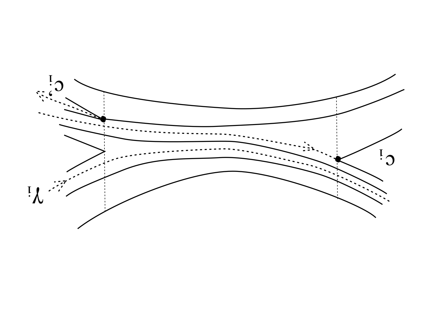
If we cut $N(h(\tau))$ along the finite collection of finite paths $\gamma_{i}$ we obtain a new surface $N_{1}(\tau,h,\varphi)$ that is obviously homeomorphic with $N(h(\tau))$. This observation implies the following lemma that appeared in [PaPe].

Lemma 3.1

Every train track map representing an element $[f]$ in the mapping class group is obtained by a finite sequence of ”elementary” splitting operations followed by a relabeling homeomorphism.

This statement is essencially obvious from the previous observation. Our goal now is to make the elementary splitting operations explicit, as well as the relabeling homeomorphism. Then we shall use these splitting operations for the reverse purpose, namely for constructing train track maps and the corresponding mapping class elements.

In their paper Papadopoulos and Penner [PaPe] Êwere interested to splitting sequences at generic train tracks, i.e. with only valency 3 vertices. For these sequences a very simple coding with 2 symbols is available, the so called R,L sequences. More recently Hamenstädt added the constraints that $(\tau,h)$ represents foliations in the principal stratum, i.e. with only triangles for the complementary components. We will not use these restrictions here, allowing the foliations to belong to more degenerate strata and encouraging the train tracks to have higher valency vertices. This enables to define explicitly splitting operations on labeled train tracks as train tracks morphisms, given by celular maps between two different train tracks that we call splitting morphisms.

Observe that splitting operations appeared also for interval exchange transformations and the Rauzy induction strategy is nothing but a very special splitting sequence at a very special class of train tracks.

A labeling is a map $\epsilon:E(\tau)\rightarrow\mathbb{A}$, where $\mathbb{A}$ is a finite alphabet. The map $\epsilon$ just names each edge. A splitting operation is defined for a given $N(h(\tau))$ at a specific cusp $C_{i}$, we want to fixe the alphabet once and for all and to avoid changing from one stratum to another. To this end we impose the following constraints:
(a) $\tau$ has at least a vertex of valency larger than 3.
(b) A splitting operation is not applied at a vertex of valency 3.
(c) At a vertex with more than 2 edges on one of it’s sides, only Êthe splittings at the extrem cusps and through the extrem edges are allowed.
(d) A splitting path do not connect a cusp of $N(h(\tau))$ to another cusp of Ê$N(h(\tau))$.

The notion of an extrem cusp or edge is clear from the context. A splitting operation is a cutting along a path $\gamma$ that connects a cusp $C_{i}$ of $N(h(\tau))$ to a point in the interior of a singular leaf of the tie foliation (condition (d)). A splitting is elementary if the path $\gamma$ do not intersects singular leaves except at it’s extrem points. The splitting operation then defines a new neighborhood $N(h^{\prime}(\tau^{\prime}))$ that is embedded into $N(h(\tau))$ and thus, via the retraction $\rho$, a map $S_{C_{i}}:(\tau,h)\leftarrow(\tau^{\prime},h^{\prime})$ (it will be written $\tau Ê\leftarrow\tau^{\prime}Ê$ if no confusion is possible).

Under the above conditions the following properties are obvious:
Every train track satisfying (a) admits some splitting operations.
The structure of the complementary components is preserved (by (d)).
ÊThe number of vertices and edges is preserved (by (b), (c), (d) ).
ÊÊThe map $S_{C_{i}}$ is injective on vertices (by (b), (c)).
Since the number of edges is fixed under the splitting operations we can fixe once and for all the alphabet $\mathbb{A}$.

Now let us consider a labeled train track $(\tau,h,\epsilon)$. We want to define explicitly the map $S_{C_{i}}$ called a splitting morphism, as a cellular map using the labels. To this end we give an arbitrary orientation to the edges in order to describe the images $S_{C_{i}}(e)$, for every edge $e\in E(\tau)$, as an edge path in $\tau$. A particular splitting morphism at a cusp $C_{i}$ is a local operation that changes the train track in a neighborhood of the vertex $v$ where $C_{i}$ is based. If $C_{i}$ is on one side of $v$ there are, at most, two possible splitting morphisms at $C_{i}$, by condition (c). Let us consider the particular case where $v$ has valency 4 with two edges on each side (see Figure Ê5), the general case is an obvious adaptation. Figure 5 shows a particular labeling and how the labeling is transformed under an elementary splitting. As observed above the transformation of the graph takes place in a neighborhood of $v$. The natural convention for the labeling of $\tau^{\prime}$ is to keep the same names as in $\tau$ for all the edges that still exist after the operation. Thus only one edge could be renamed after the operation but the alphabet is fixed and then only one name is available. This convention explains the unambiguous labeling of Figure 5.

Figure 5: ÊThe splitting morphisms.

In the particular cases of Figure 5, i.e. with two edges (labeled c or d) on the opposite side of $C_{i}$, there are two possible splittings (case I or II in Figure 5) and the two morphisms are given by the following maps :

$S_{C_{i}}:\tau^{\prime}\rightarrow\tau$

$aÊ\rightarrow Êa.c,Ê\hskip 8.53581ptÊÊxÊ\rightarrow x,$ for all $x\neq a$, in case I

$bÊ\rightarrow Êb.d,Ê\hskip 8.53581ptÊxÊ\rightarrow x,$ for all $x\neq b$, in case II.

Lemma 3.1 can be rephrased as:
Any train track map $\varphi:\tau\rightarrow\tau$ representing an element in the mapping class group is obtained as a composition of splitting morphisms $\{ÊS_{C_{i_{1}}},\cdots,ÊÊS_{C_{i_{n}}}\}$, followed by a train track automorphism Ê $\alpha$:

$\tau Ê\stackrel{{\scriptstyle S_{C_{i_{1}}}}}{{\leftarrow}}\tau_{1}\stackrel{{\scriptstyle S_{C_{i_{2}}}}}{{\leftarrow}}\tau_{2}\cdots\stackrel{{\scriptstyle S_{C_{i_{n}}}}}{{\leftarrow}}\tau_{n}\simeq\tau\stackrel{{\scriptstyle\alpha}}{{\leftarrow}}\tau$.

Along the sequence of splitting morphisms, each $\tau_{j}$ has a well defined labeling, obtained inductively from the one of $\tau$. In particular $\tau_{n}$ is homeomorphic with $\tau$ but the labeling is a priori different. The train track automorphism $\alpha$ induces, in particular, a relabeling. Observe that a given train track map might admits several splitting morphisms decompositions.

Let us now make an obvious but crutial observation for the fixed point problem. The first observation is that the train track automorphism might not be unique, that’s the case if $\tau$ admits a symmetry, i.e. a non trivial automorphism group. The splitting morphisms that are given above, together with lemma 2.3, shows that if $\tau^{\prime}$ is homeomorphic with $\tau$ and if the relabeling is the trivial one then many fixed points will exist. Therefore to avoid fixed points it is highly desirable for the train track $\tau$ to admit a non trivial automorphism group.

4 Construction of examples.

4.1 A preliminary example.

From the previous sections we are looking for a train track map $\varphi:\tau\rightarrow\tau$ satisfying the following properties :
(i) $\tau$ is orientable,
(ii) $\tau$ has a non trivial automorphism group,
(iii) $\varphi$ has no fixed points.

Of course the first two conditions are quite easy to satisfy and the real difficulty is to find a map $\varphi$ as a sequence of splitting morphisms satisfying (iii). The first example is obtained by an experiment on the labeled train track of Figure 6.

Figure 6: The initial labeled train track.

On this train track the orientability is obvious to check, at each vertex there is an orientation of the incident edges that is compatible with the In/Out partition of the smooth structure. The symmetry is of order two which means that the graph has two parts that are exchanged by the symmetry (an involution). With the labeling of ÊFigure 6 this involution is Êgiven by $\{a,b,c,d,k,l\}\rightarrow\{g,h,i,j,e,f\}$. Any splitting sequence produces a sequence of maps that increases the length of the image of some edge. Our main strategy is avoid any image to be ”too long” on it’s symmetric part.

The difficulty for constructing examples is easily expressed by observing that the train track $\tau$ of Figure 6 has 12 cusps and the maximal number of possible splittings at any train track along the sequence is 24. Thus the number of possibilities at each step is of order 24 and the growth is exponential with respect to the length of the sequence.

For describing the sequence we introduce a simple notation. First notice that starting from a labeled and oriented train track as in Figure 6 implies that after each splitting step, the new train track has a well defined orientation and labeling. A given edge $x\in\tau$, being oriented, has an initial vertex $i(x)$ and a terminal vertex $t(x)$. The splitting morphisms of Figure 5 can be described as ”sliding” the terminal part of $"a"$ over the initial part of $"c"$ in case I or the terminal part of $"b"$ over the initial part of $"d"$ in case II. For this reason the two possible morphisms are denoted $\frac{t(a)}{i(c)}$ or $\frac{t(b)}{i(d)}$, this notation is unambiguous and gives at the same time the cusp and the morphism.

The very first sequence we want to describe on the labeled train track of Figure 6, with this notation, is the following:

$\Big\{\frac{i(b)}{t(l)};\frac{t(b)}{i(d)};\frac{t(k)}{i(f)};\frac{i(k)}{t(j)};\frac{t(e)}{i(l)};\frac{t(c)}{i(a)};\frac{i(c)}{t(a)};\frac{i(e)}{t(d)};\frac{i(h)}{t(f)};Ê\frac{t(h)}{i(j)};\frac{t(f)}{i(g)};\frac{i(j)}{t(g)}\Big\}$.

The surprise is that such a short sequence gives back the same topological train track. The composition of all these elementary splittings gives the image train track as shown by Figure 7. The figure should be understood as embedded in the regular neighborhood of the topological Ê(i.e. without the labels) train track $\tau$ of Figure 6.

We observe that this image is indeed the same topological train track but with a different labeling, given by Figure 8. In addition, since the automorphism group has order two, then there are two ways to relabel the train track by a train track automorphism, this is shown in Figure 8.

Figure 7: The image train track, after the sequence of splittings, in the regular neighborhood of $\tau$.

Figure 8: The two possible labelings.

Let us now analyse this example. First a very simple computation shows that the train track $\tau$ is embedded in a surface of genus 3 with 2 boundary components, that are the boundary components of the regular neighborhood of $\tau$. With the labeling of Figure 8 these two boundary components are written as cyclic edge paths on $\tau$ given by :

$\partial_{1}=ij\overline{h}\overline{d}ea\overline{c}\overline{l}bf\overline{g}\overline{k}$ Êand $\partial_{2}=iÊ\overline{k}\overline{g}jb\overline{d}\overline{c}ae\overline{l}\overline{h}f$.

The notation $\overline{x}$ means that the oriented edge $x$ is crossed by the path with the opposite orientation.

In order to make the map $\varphi$ explicit we just have to chose one of the two possible labelings of Figure 8 and read the image of each edge as an edge path on $\tau$. Using the identification II of Figure 8 for $\tau$ and reading the paths of Figure 7 on this labeled train track gives the following celular map $\varphi_{1}$ :

$\bullet$ Ê$a\mapsto k,\hskip 5.69054pt$ $\bullet$ $b\mapsto fij,\hskip 5.69054pt$ $\bullet$ $c\mapsto kgk,\hskip 5.69054pt$ $\bullet$ $d\mapsto j,\hskip 5.69054pt$ $\bullet$ $e\mapsto jbf,\hskip 5.69054pt$ $\bullet$ $f\mapsto la,\hskip 5.69054pt$
$\bullet$ $g\mapsto a,\hskip 5.69054pt$ $\bullet$ Ê$h\mapsto lcd,\hskip 5.69054pt$ $\bullet$ $i\mapsto e,\hskip 5.69054pt$ $\bullet$ Ê$j\mapsto Êad,\hskip 5.69054pt$ $\bullet$ Ê$k\mapsto Êdhl,\hskip 5.69054pt$ $\bullet$ $l\mapsto f$.

The first very good news is that no letter appears in it’s own image. This is enougth to prove that $\varphi_{1}$ has no fixed points by lemma 2.3. This implies that the homeomorphism that $\varphi_{1}$ represents on the genus 3 surface with 2 boundary components has no fixed points in it’s interior. We need now to check what happens for the boundaries. A simple computation shows that $\varphi_{1}(\partial_{i}),i=1,2$ is a word that cyclically reduces to a cyclic permutation of $\partial_{i},i=1,2$. Thus each boundary component is invariant under $\varphi_{1}$, i.e. the image is isotopic to itself, as a closed curve, but with a non trivial rotation because of the cyclic permutation.

This proves first that $\varphi_{1}$ is induced by a homeomorphism $f_{1}$ Êand $f_{1}$ has no fixed points on the genus 3 surface with 2 boundary components.

Now we observe that each boundary curve $\partial_{i},i=1,2$, as an edge path in $\tau$, has six cusps and thus is a union of six periodic Nielsen paths (lemma 2.4). The same $\varphi_{1}$ defines a homeomorphism $\widehat{f_{1}}$ on a closed surface of genus 3 with two 6-prong singularities and, since $\varphi_{1}(\partial_{i})\sim Ê\partial_{i},i=1,2$, these two singularities are fixed under $\widehat{f_{1}}$. In addition, for each of these two fixed points, the six separatrices are permuted non trivially under $\widehat{f_{1}}$ since Ê${f_{1}}_{|\partial_{i}}$ is a non trivial rotation (see [FL] for more details). The transformation of the surface with boundaries to a closed surface is similar to the ”zipped rectangles” operation of Veech [Ve], the zipping being given here by the periodic Nielsen paths.

It seems that we have an anwer to our question…We obtain a homeomorphism without fixed points on a surface with boundaries or without fixed points of negative index on a closed surface both fixing an orientable measured foliation.
The bad news is that these two homeomorphisms are not pseudo-Anosov… Indeed the incidence matrix $M(\tau,\varphi_{1})$ fails to be irreducible. This can be checked for instance by observing that the proper subgraph $\tau_{0}$ of $\tau$ that consists of the edges $\{a,c,d,f,g,h,j,k,l\}$ is invariant under $\varphi_{1}$ and therefore the matrix $M(\tau,\varphi_{1})$ has a block structure and proposition 2.2 does not apply.

4.2 Infinite sequence of pseudo-Anosov homeomorphisms.

The idea to create a sequence of pseudo-Anosov homeomorphisms from the map $\varphi_{1}$ already obtained, is to compose it with an infinite sequence of Dehn twists along a curve $C$ that belongs to only one part of $\tau$, with respect to the symmetry, and do not change the map on the symmetric part of $\tau$. In other words this particular curve $C$ has the property that it’s image under the homeomorphism $f_{1}$ is disjoint from itself. An arbitrary train track map will certainly not admit such a curve. Our previous example admits a curve, given in the labeled train track of Figure 8 by the edge path $C=i.g$ whose image is $\varphi_{1}(C)=C^{\prime}=e.a$ that is disjoint from $C$.

Let us describe this particular Dehn twist on $\tau$ with the labeling of Figure 8 as a splitting sequence. It is given by :

$\Big\{\frac{t(f)}{i(i)};\frac{i(j)}{t(i)};\frac{i(k)}{t(g)}Ê;Ê\frac{t(k)}{i(g)}\Big\}$. Ê

The new train track $\tau^{\prime}$ is homeomorphic to $\tau$ with a relabeling map $\alpha:\tau\rightarrow\tau^{\prime}$ given by:

$i\rightarrow g,\hskip 5.69054ptg\rightarrow i,Êx\rightarrow x$ for all $x\neq\{i,g\}$.

The image of $\tau^{\prime}$ is shown by Figure 9 and the twist map, along the closed curve $(i,g)$, Ê$T(i,g):\tau^{\prime}\rightarrow\tau$ is given by:

$f\rightarrow f.i,\hskip 5.69054ptj\rightarrow i.j,\hskip 5.69054ptk\rightarrow g.k.g$ Êand $x\rightarrow x$ for all $x\neq\{f,j,k\}$ .

Figure 9: ÊThe Dehn twist $T(i,g)$.

The composition of all these maps : $Ê\hskip 14.22636pt\varphi_{2}:\tau^{\prime}Ê\stackrel{{\scriptstyle T(i,g)}}{{\rightarrow}}\tau\stackrel{{\scriptstyle\varphi_{1}}}{{\rightarrow}}\tau\stackrel{{\scriptstyle\alpha}}{{\rightarrow}}\tau^{\prime}$ gives the following :

$\bullet$ Ê$a\mapsto k,\hskip 5.69054pt$ $\bullet$ $b\mapsto fgj,\hskip 5.69054pt$ $\bullet$ $c\mapsto kik,\hskip 5.69054pt$ $\bullet$ $d\mapsto j,\hskip 5.69054pt$ $\bullet$ $e\mapsto jbf,\hskip 5.69054pt$ $\bullet$ $f\mapsto lae,\hskip 5.69054pt$
$\bullet$ $g\mapsto a,\hskip 5.69054pt$ $\bullet$ Ê$h\mapsto lcd,\hskip 5.69054pt$ $\bullet$ $i\mapsto e,\hskip 5.69054pt$ $\bullet$ Ê$j\mapsto ead,\hskip 5.69054pt$ $\bullet$ Ê$k\mapsto adhla,\hskip 5.69054pt$ $\bullet$ $l\mapsto f$.

We check immediately that $\varphi_{2}$ has no fixed points by lemma 2.3. The two boundary components are, as before, invariant up to homotopy under $\varphi_{2}$, and the induced rotations are non trivial. We finally check that the incidence matrix $M(\tau^{\prime},\varphi_{2})$ is irreducible. Therefore, from proposition 2.2, $\varphi_{2}$ represents a pseudo-Anosov homeomorphism either on a surface of genus 3 with 2 boundary components, without fixed points, or on a closed surface of genus 3 with two fixed 6-prong singularities of positive index (the separatrices are permutted). In both cases the pseudo-Anosov have orientable invariant foliations. We thus obtained our first example.

The construction of an infinite sequence is now quite clear from this example, we just have to iterate the twist map. In fact since the two train tracks $\tau$ and $\tau^{\prime}$ differs just by an order two relabeling ( $\alpha$) there is another sequence of splitting for the next twist that we denote $T(g,i):\tau\rightarrow\tau^{\prime}$ and is given by the following splitting sequence:

$\Big\{\frac{t(f)}{i(g)};\frac{i(j)}{t(g)};\frac{i(k)}{t(i)}Ê;Ê\frac{t(k)}{i(i)}\Big\}$. Ê

The next map in the sequence is obtained by the composition: $Ê\hskip 14.22636pt\varphi_{3}:\tau Ê\stackrel{{\scriptstyle T(g,i)}}{{\rightarrow}}\tau^{\prime}Ê\stackrel{{\scriptstyle T(i,g)}}{{\rightarrow}}\tau\stackrel{{\scriptstyle\varphi_{1}}}{{\rightarrow}}\tau Ê$.
Observe that the relabeling $\alpha$ is not needed here and this map $\varphi_{3}$ is written combinatorially as :

$\bullet$ Ê$a\mapsto k,\hskip 5.69054pt$ $\bullet$ $b\mapsto fij,\hskip 5.69054pt$ $\bullet$ $c\mapsto kgk,\hskip 5.69054pt$ $\bullet$ $d\mapsto j,\hskip 5.69054pt$ $\bullet$ $e\mapsto jbf,\hskip 5.69054pt$ $\bullet$ $f\mapsto laea,\hskip 5.69054pt$
$\bullet$ $g\mapsto a,\hskip 5.69054pt$ $\bullet$ Ê$h\mapsto lcd,\hskip 5.69054pt$ $\bullet$ $i\mapsto e,\hskip 5.69054pt$ $\bullet$ Ê$j\mapsto aead,\hskip 5.69054pt$ $\bullet$ Ê$k\mapsto eadhlae,\hskip 5.69054pt$ $\bullet$ $l\mapsto f$.
This new map $\varphi_{3}$ satisfies exactly the same properties than $\varphi_{2}$.

The simplest infinite sequence can then be written as: $Ê\hskip 14.22636pt\varphi_{2n+1}:\Big\{\tau Ê\stackrel{{\scriptstyle T(g,i)}}{{\rightarrow}}\tau^{\prime}Ê\stackrel{{\scriptstyle T(i,g)}}{{\rightarrow}}\tau{\Big\}}^{n}\stackrel{{\scriptstyle\varphi_{1}}}{{\rightarrow}}\tau Ê$,
where the notation $\{...\}^{n}$ is the natural $n$ times composition of splitting morphisms. The combinatorial map is given on the train track $\tau$ of Figure 8, with identification II, as:

$\bullet$ Ê$a\mapsto k,\hskip 5.69054pt$ $\bullet$ $b\mapsto fij,\hskip 5.69054pt$ $\bullet$ $c\mapsto kgk,\hskip 5.69054pt$ $\bullet$ $d\mapsto j,\hskip 5.69054pt$ $\bullet$ $e\mapsto jbf,\hskip 5.69054pt$ $\bullet$ $f\mapsto la(ea)^{n},\hskip 5.69054pt$
$\bullet$ $g\mapsto a,\hskip 5.69054pt$ $\bullet$ Ê$h\mapsto lcd,\hskip 5.69054pt$ $\bullet$ $i\mapsto e,\hskip 5.69054pt$ $\bullet$ Ê$j\mapsto(ae)^{n}ad,\hskip 5.69054pt$ $\bullet$ Ê$k\mapsto(ea)^{n}dhl(ae)^{n},\hskip 5.69054pt$ $\bullet$ $l\mapsto f$.

These maps satisfy all the same properties than $\varphi_{3}$ and this completes the proof of our theorem. The fixed point property is obvious to check by inspection. The pseudo-Anosov property is checked inductively. The fact that all these examples belong to the same stratum comes from the fact that the boundary curves $\partial_{1},\partial_{2}$ have the same 6-cusps structure. Observe that the maps in this sequence have incidence matrices whose norm is strictly growing and thus the growth rate of the corresponding pseudo-Anosov goes to infinity.

For completeness, the maps $\varphi_{2n+1}$ is written, as a splitting sequence with the above notations as:

$\Big\{ÊÊ\big\{\frac{i(b)}{t(l)};\frac{t(b)}{i(d)};\frac{t(k)}{i(f)};\frac{i(k)}{t(j)};\frac{t(e)}{i(l)};\frac{t(c)}{i(a)};\frac{i(c)}{t(a)};\frac{i(e)}{t(d)};\frac{i(h)}{t(f)};Ê\frac{t(h)}{i(j)};\frac{t(f)}{i(g)};\frac{i(j)}{t(g)}\big\}\big\{\frac{t(f)}{i(i)};\frac{i(j)}{t(i)};\frac{i(k)}{t(g)}Ê;Ê\frac{t(k)}{i(g)}.\frac{t(f)}{i(g)};\frac{i(j)}{t(g)};\frac{i(k)}{t(i)}Ê;Ê\frac{t(k)}{i(i)}\big\}^{n}\Big\}$.

With the same basic ingredients there is another infinite sequence that is given by the composition: $Ê\hskip 14.22636pt\psi_{n}:Ê\tau Ê\stackrel{{\scriptstyle\varphi_{1}}}{{\rightarrow}}\Big\{\tau Ê\stackrel{{\scriptstyle T(g,i)}}{{\rightarrow}}\tau^{\prime}Ê\stackrel{{\scriptstyle T(i,g)}}{{\rightarrow}}\tau{\Big\}}^{n}Ê$,

The corresponding combinatorial maps on the labelled train track of Figure 8 are given by:
$\bullet$ Ê$a\mapsto(ig)^{n}k(gi)^{n},\hskip 5.69054pt$ $\bullet$ ÊÊ$b\mapsto f(ig)^{n}Êi(gi)^{n}Êj,\hskip 5.69054pt$ $\bullet$ ÊÊ$c\mapsto(ig)^{n}k(gi)^{n}ÊgÊ(ig)^{n}ÊkÊ(gi)^{n},\hskip 5.69054pt$ $\bullet$ ÊÊÊ$d\mapsto(gi)^{n}Êj,\hskip 5.69054pt$
$\bullet$ ÊÊÊÊ$e\mapsto Ê(gi)^{n}jbf(ig)^{n},\hskip 5.69054pt$ $\bullet$ ÊÊÊ$f\mapsto la,\hskip 5.69054pt$ $\bullet$ ÊÊÊÊ$g\mapsto a,\hskip 5.69054pt$ $\bullet$ ÊÊÊÊÊ$h\mapsto lcd,\hskip 5.69054pt$ $\bullet$ ÊÊÊÊÊ$i\mapsto e,\hskip 5.69054pt$ $\bullet$ ÊÊÊÊÊÊ$j\mapsto Êad,\hskip 5.69054pt$ $\bullet$ ÊÊÊÊ$k\mapsto Êdhl,\hskip 5.69054pt$
$\bullet$ ÊÊÊÊ$l\mapsto f(ig)^{n}\hskip 5.69054pt$.

This sequence is different from the previous one and all these maps satisfy again the same properties with respect to the fixed points question.

These sequences are really very special in particular because the Dehn twists are directly realized as splitting sequences. Similar examples on other surfaces should be obtained the same way Êbut each surface and each stratum requires a specific study. For genus two surfaces this approach by hand did’nt succeed yet. ÊA systematic study of all the pseudo-Anosov homeomorphisms on a given stratum would require to develop the specific train track automata theory. For practical purposes such automata are huge and an algorithmic description is probably necessary, in particular for counting problems.

References

[ALM] ÊL.Alseda, J.Llibre, M.Misiurewicz. Combinatorial dynamics and entropy in dimension one. World scientific, Advances series in non linear dynamics, Vol 5, (1993).

[A] P.Arnoux. Un exemple de semi-conjugaison entre un échange d’intervalles et une translation du tore. Bull. Soc. Math. France, 116 (1988), nÁ4, pp 489-500.

æ[A.Y] P. Arnoux , J.C.æYoccoz. æConstruction de diff?omorphismes pseudo-Anosov.æ C. R. Acad. Sci. Paris S?r. I Math.æ292æ(1981), no. 1, 75–78.æ

[BH] M.Bestvina, M.Handel. Train tracks for surface homeomorphisms. Topology, 34 (1995) 109-140.

[Bo] P.Boyland. Topological methods in surface dynamics. Top. Appl. Ê58, ( 1994), pp 223-298.

[CB] A.Casson, S.Bleiler. Automorphisms of surfaces after Nielsen and Thurston Cambridge University Press, Cambridge (1988).

[FLP] A.Fathi, F.Laudenbach, V.Poenaru. Travaux de Thurston sur les surfaces Astérisque vol 66-67 (1979).

[FL] J.Fehrenbach, J.Los. Roots, symmetry and conjugacy of pseudo-Anosov homeomorphims. Preprint 2007.

[Ha] U.Hamenstädt. Train tracks and the Gromov boundary of the complex of curves in ”Spaces of Kleinian groups” Ê(Y.Minsky, M.Sakuma, C.Series, Eds.) Lond. Math.Soc..Lec.Notes 329 (2005).

[KLS] K.H.Ko, J.Los, W.T.Song. Entropy of braids. Jour. Knot. Theo. ramif, 11, 4, (2002), 647-666.

[Lo] J.Los. On the forcing relation for surface homeomorphisms. Publ.Math. IHES, 85, (1997), 5-61.

[PaPe] A.Papadopoulos, ÊR.Penner. A characterization of Pseudo-Anosov foliations. ÊPac. Journ.Math. 130, 2 (1987), pp 359-377.

[PH] R.C.Penner with J.L.Harer. Combinatorics of train tracks Annals of Math.Studies, 125, (1992).

[Ra] G.Rauzy. Echanges d’intervalles et transformations induites. Acta.Arith. 34, (1979), 315-328.

[Th] W. Thurston. On the geometry and dynamics of diffeomorphisms on surfaces, Bull. A.M.S. 19 (1988) pp. 417-431.

[Ve] ÊW.A.Veech. Teichmüller geodesic flow. Annals of Math. 124, (1986), 441-530.

[Wi] R.Williams. One dimentional non wandering sets. Topology, 6, ( 1967), 473-487.

Laboratoire d’Analyse, Topologie, Probabilité (LATP), UMR CNRS 6632
Université de Provence,
39 rue F.Joliot Curie
13453 Marseille Cedex 13,
France.
E-mail adresse : los@cmi.univ-mrs.fr