Real-time synchronization feedbacks for single-atom frequency standards Thanks: This work was partially supported by the ”Agence Nationale de la Recherche” (ANR), Projet Blanc CQUID number 06-3-13957.

Abstract

Simple feedback loops, inspired from extremum-seeking, are proposed to lock a probe-frequency to the transition frequency of a single quantum system following quantum Monte-Carlo trajectories. Two specific quantum systems are addressed, a 2-level one and a 3-level one that appears in coherence population trapping and optical pumping. For both systems, the feedback algorithm is shown to be convergent in the following sense: the probe frequency converges in average towards the system-transition one and its standard deviation can be made arbitrarily small. Closed-loop simulations illustrate robustness versus jump-detection efficiency and modeling errors.

1 Introduction

The SI second is defined to be “the duration of 9 192 631 770 periods of the radiation corresponding to the transition between the two hyperfine levels of the ground state of the caesium 133 atom” [1]. A primary frequency standard is a device that realizes this definition. Extremum seeking techniques (see, e.g, [3] for a recent exposure) are usually used in high precision spectroscopy to achieve frequency lock with an atomic transition frequency [15, 14]. For micro atomic-clocks [9] synchronization is achieved when the output signal of a photo-detector is maximum (or minimum). This characterizes perfect resonance between the probe laser frequency with the atomic one. As sketched on figure 1, such synchronization feedback schemes are based on a modulation of the probe frequency, the input $u$, with a sinusoidal variation $a\sin(\omega t)$ of small amplitude $a$ and fixed (low) frequency $\omega$, on a high-pass filtering (transfer function $\frac{s}{s+h}$) of the photo-detector signal (the output $y$), on a multiplier and finally an integrator giving the mean input value.

Fig. 1: The basic extremum seeking feedback loop for a non-linear static system $y=f(u)$ ($s=\frac{d}{dt}$ is the Laplace variable and $(h,k,a,\omega)$ are constant design parameters).

In such synchronization scheme the system corresponds to a population of identical quantum systems with few mutual interactions (the vapor cell) having reached its asymptotic statistical regime described by a density matrix solution of a static Lindblad-Kossakovski master equation. In this paper, we propose to adapt this feedback strategy to a single quantum system. Such a system cannot be described by a static non-linear input/output map but it obeys a stochastic jump dynamics [5, 8]. The output signal is no more continuous since it corresponds to a counter giving the jump times. As shown in [4], all the spectroscopic information and in particular the value of the atomic transition frequency are contained in the statistics of these jump-time series. Thus it is not surprising that such feedback loops are possible. The contribution of this paper is to propose for the first time (as far as we know) a real-time synchronization feedback scheme that can be implemented on electronic circuits of similar complexity to those used for extremum-seeking loops. In the feedback loop, we avoid thus the use of quantum filters [7] and records of jump-times sequences required by usual statistical treatments.

We consider here two kinds of quantum systems. The first system is the simplest one we can imagine. It has a stable ground state and an excited unstable one. These two states are in interaction with a quasi-resonant electromagnetic field characterized by a complex amplitude $u+\imath v$ and a frequency $\Omega$ close to the transition frequency between the ground and excited states. The measure corresponds then to the photon emitted by the excited state when it relaxes to the ground state by spontaneous emission. The complex amplitude is then modulated according to $\bar{u}+\imath\bar{v}\cos(\omega t)$ ($(\bar{u},\bar{v})$ positive parameters, modulation frequency $\omega\ll\Omega$). The synchronization feedback (playing the role of the integrator in figure 1) corresponds essentially to the recurrence $\Omega_{N+1}=\Omega_{N}-\delta\sin(\omega t_{N})$ where $N$ is the jump-index, $t_{N}$ the jump-time, and $\Omega_{N}$ the probe frequency between time $t_{N-1}$ and time $t_{N}$ ($\delta$ positive parameter). The second system corresponds to a typical $\Lambda$-system appearing in coherent population trapping phenomena and optical pumping [2]. Such 3-level configurations are also present in micro atomic clocks. The synchronization feedback is very similar to the previous one (see subsection 3.2). Both feedback schemes are illustrated by closed-loop quantum Monte-Carlo simulations and rely on two formal results (theorems 1 and 3) ensuring the convergence of the mean frequency de-tuning to $0$ with a standard deviation that can be made arbitrary small.

The model considered in this paper corresponds to quantum Monte Carlo trajectories. Note that, although quantum trajectories represent a useful simulation method for the quantum master equation, they are interesting in their own right, since they model the measurement process itself and the resulting conditioned dynamics. In fact, some of the original work that motivated quantum trajectories [4, 17] was to understand experiments on quantum jumps (for atoms with a vee configuration) [13, 16]. Therefore, through the paper, one should understand the “quantum Monte Carlo” trajectories as the model and not as a numerical method. We refer to [8] for more details.

The paper is organized as follows. Section 2 is devoted to the two-level system: the stochastic jump dynamics are depicted in subsection 2.1; the synchronization feedback is detailed in subsection 2.2; the remaining two subsections deal with closed-loop simulations illustrating theorem 1. Section 3 deals with the $\Lambda$-system and admits exactly the same structure as section 2. The two last sections 4 and 5 are devoted to the proofs of the two main results, theorems 1 and 3.

The authors thank Guilhem Dubois from LKB and André Clairon from SYRTE for interesting discussions, suggestions and references in physics journals.

2 The two-level system

2.1 Monte-Carlo trajectories

This 2-level system is defined on the Hilbert space ${\mathcal{H}}=\text{span}\left\{\left|g\right>,\left|e\right>\right\}$: the ground state $\left|g\right>$ is stable whereas the excited state $\left|e\right>$ is unstable with life time $1/\Gamma$ and relaxes to $\left|g\right>$. The system is submitted to a near-resonant laser field whose complex amplitude is assumed to be slowly variable with respect to the transition frequency. Its dynamics are stochastic with quantum Monte-Carlo trajectories [8] described here below.

In the absence of quantum jump, the density matrix $\rho$ evolves through the dynamics

$$\frac{d}{dt}\rho=-\imath[\frac{H}{\hbar},\rho]-\frac{1}{2}\left\{L^{\dagger}L,\rho\right\}+\text{Tr}\left(L^{\dagger}L\rho\right)\rho$$

where $\left\{L^{\dagger}L,\rho\right\}=L^{\dagger}L\rho+\rho L^{\dagger}L$ stands for the anti-commutator. Note that, the nonlinear term in the above dynamics is being added to ensure that the density matrix remains normalized to trace 1. In fact, the usual formulation for quantum Monte Carlo trajectories uses the wavefunction language and normalizes the wavefunction at each step. Here, without loss of generality and for simplicity sakes we have translated these dynamics to the density matrix one.

The Hamiltonian $\frac{H}{\hbar}=\frac{\Delta}{2}\sigma_{z}+u\sigma_{x}+v\sigma_{y}$ is attached to the conservative part of the dynamics: $(\sigma_{x},\sigma_{y},\sigma_{z})$ are the Pauli matrices; $\Delta$ denotes the laser-atom detuning; $u$ and $v$ are the real coefficients of the complex laser amplitude. The jump operator $L=\sqrt{\Gamma}\left|g\right>\left<e\right|,$ is associated to the dissipative dynamics with $\Gamma>0$ denoting the decoherence rate. Note that, the above Hamiltonian is the result of a common rotating wave approximation, where the detuning and the decoherence rates are smaller than the transition frequencies of the atom [8].

At each time step $dt$ the system may jump on the ground state $\left|g\right>\left<g\right|$ with a probability given by

$$p_{\text{jump}}(\rho\rightarrow\left|g\right>\left<g\right|)=\text{Tr}\left(L^{\dagger}L\rho\right)dt=\Gamma\text{Tr}\left(\left|e\right>\left<e\right|\rho\right)dt=\Gamma~\left<e\right|\rho\left|e\right>dt.$$

Each jump is associated to the spontaneous emission of a photon that is detected by the photo-detector: the measurement is just a simple click and we know that just after the click the system is at the ground state, i.e., $\rho=\left|g\right>\left<g\right|$.

In the sequel, we will use this stochastic dynamics in the $\Gamma$-scale. This just consists in replacing $u$ by $u\Gamma$, $v$ by $v\Gamma$, $\Delta$ by $\Delta\Gamma$, and $t$ by $t/\Gamma$ in the equations. In this de-coherence time-scale, the density matrix $\rho$ evolves through the dynamics

$$\frac{d}{d\bar{t}}\rho=-\imath\left[\frac{\Delta}{2}\sigma_{z}+u\sigma_{x}+v\sigma_{y},\rho\right]-\frac{1}{2}\left\{\left|e\right>\left<e\right|,\rho\right\}+\left<e\right|\rho\left|e\right>\rho$$ (1)

and the jump probability between $t$ and $t+dt$ reads

$$p_{\text{jump}}(\rho\rightarrow\left|g\right>\left<g\right|)=\left<e\right|\rho\left|e\right>dt.$$ (2)

Just after each jump, $\rho$ coincides with $\left|g\right>\left<g\right|$. The atom/laser detuning is $\Delta$ and the laser complex amplitude is $u+\imath v$.

2.2 The synchronization feedback

We consider here the two-level system described, in the decoherence time-scale, by (1) (2). The quantum jumps lead to the emission of photons that will be detected with a certain efficiency $\eta\in(0,1]$.

The main goal of this paper is to provide a real-time algorithm so that, using the information obtained through the detected photons, we can synchronize the laser with the atomic transition frequency and therefore make $\Delta$ converge to zero.

Note that, in practice we have a certain knowledge of the transition frequency and therefore, we can always tune our laser so that the detuning $|\Delta|$ does not get larger than a fixed constant $C$.

In the aim of providing a synchronization algorithm inspired from extremum-seeking, we consider a laser field amplitude of the form

$$u=\bar{u},\quad v=\bar{v}\cos(\omega t)$$

where the modulation frequency $\omega$ is of order $1$ but where $\bar{u}$ and $\bar{v}$ are small: $\bar{u},\bar{v}\ll 1$.

The main strategy for the correction of the detuning is to wait for the matured quantum jumps (clicks of the photo-detector). This means that we choose a certain time constant $T\gg 1$ and if the distance between two jumps is more than $T$, we will correct the detuning according to the time when the second jump happens. Note that, one can easily show that these matured quantum jumps, almost surely, happen within a finite horizon. Here is the explicit feedback algorithm:

1. Start with a certain detuning $\Delta_{0}$ with $|\Delta_{0}|\leq C$ and set the switching parameter $S=0$ and the counter $N=0$.

2. Wait for a first click and meanwhile evolve the switching parameter through $\frac{d}{dt}S=1$.

3. If the click happens while $S\leq T$ then switch the parameter $S$ to zero and go back to the step 2.

4. If the click happens while $S>T$ then switch the parameter $S$ to zero, change the counter value to $N+1$, correct the detuning $\Delta_{N}$ as follows:

   $$\left\{\begin{aligned} &\Delta_{N+1}=\Delta_{N}-\delta\sin(\omega t)\qquad&\text{if }|\Delta_{N}-\delta\sin(\omega t)|\leq C,\\ &\Delta_{N+1}=C,\qquad&\text{otherwise}\end{aligned}\right.$$

   and go back to the step 2.

Here we have chosen the correction gain $\delta\ll 1$. Our claim is that such an algorithm provides an approximate synchronization of laser frequency: given any small $\epsilon$, we can adjust the design parameters $\bar{u}$, $\bar{v}$ and $\bar{\delta}$ small enough such that with the above algorithm, the detuning $\Delta_{N}$ converges in average to an $O(\epsilon^{2})$-neighborhood of 0 with a deviation of order $O(\epsilon)$ (in the $\Gamma$-scale): according to theorem 1, it suffices to take $\bar{u},\bar{v}\sim\epsilon$, $\delta\sim\epsilon^{2}$ and $(\omega,C)$ such that $4\omega^{2}>1+4C^{2}$ to ensure such convergence. In theorem 1, the ”dead-time” $T$ between two jumps is chosen mostly for technical reasons during the proof of theorem 1. It is related to the convergence time for the jump-free dynamics (1) starting with $\left|g\right>\left<g\right|$ towards an $\epsilon^{4}$-neighborhood of its asymptotic regime. Since the convergence is exponential, $T$ is linear in $-\log\epsilon$, this explain the fact that we can choose $T$ around $1$, even if $\epsilon$ is very small. However, in simulation, we have observed no convergence difference between $T>0$ large (around $10$) and $T=0$. Therefore, this dead time does not seem to be necessary in practice and one can take it simply to be 0. Finally, notice that, such algorithm is very simple and can be implemented via a standard electronic circuit. Indeed, the feedback loop only adapts the atom/laser detuning $\Delta$ that is of several orders of magnitude smaller that the optical transition frequency involving femto-second time-scales. For the two-level system, the adaptation update frequency is directly related to the time-interval between detector clicks and thus is less than $\Gamma$, the inverse of the life time of the unstable excited state. Since, in several physical situations [14, 15], $\Gamma$ lies in the radio frequency domain, the adaptation algorithm can be realized via a simple analogue circuit in the GHz range.

2.3 Numerical simulations

Let us now show the performance of this algorithm on some simulations. For the simulations of Figure 2, we take ($\Gamma=1$ in the decoherence time-scale)

$$C=1/2,\quad\eta=0.9,\quad\bar{u}=\bar{v}=6.0~10^{-2},\quad\omega=1.0,\quad\delta=9.0~10^{-4}.$$

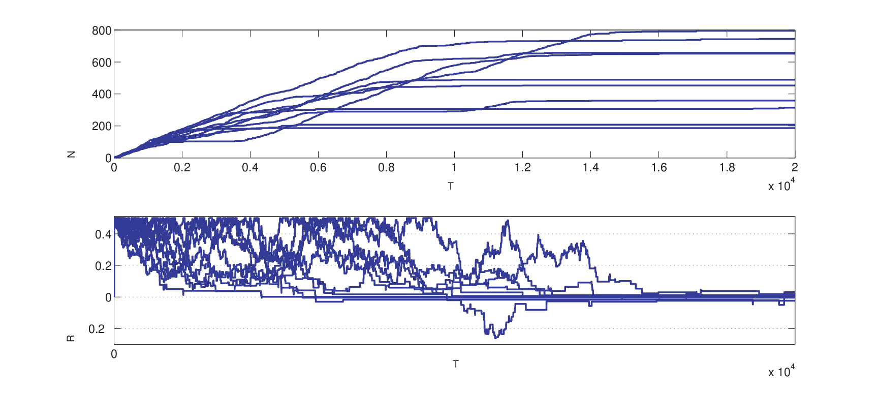
Figure 2 correspond to 10 random trajectories of the system starting with the same initial condition $\rho_{0}=\left|g\right>\left<g\right|$ and detuning $\Delta_{0}=C=1/2$. The first plot provides the number of clicks (quantum jumps) while the second one gives the evolution of the detuning $\Delta_{N}$. As it can be noted, the detuning converge to $0$ in average with a standard deviation of order $\epsilon$ (here $\epsilon\sim 10^{-2}$). In these simulations, we take the parameters $T=0$.

Fig. 2: The detuning evolution versus the number of quantum jumps for the synchronization algorithm of Subsection (2.2).

2.4 Formal result

The proof of the following theorem underlying the above simulations is given in section 4. we have the following theorem

Theorem 1.

Consider the Monte-Carlo trajectories described by (1)-(2). Assume a perfect jump-detection efficiency $\eta=1$ and take the synchronization-feedback presented in subsection 2.2 with

$$\overline{u},\overline{v}\sim\epsilon\ll 1.$$ (3)

Assume that

$$\delta\sim\epsilon^{2},\quad 4C^{2}+1<4\omega^{2}.$$ (4)

We can fix then the dead-time $T$ in the algorithm large enough so that:

$$\limsup_{N\rightarrow\infty}{\mathbb{E}}(\Delta_{N}^{2})\leq O(\epsilon^{2}).$$ (5)

Corollary 2.

Under the assumptions of the Theorem 1, one has

$$\limsup_{N\rightarrow\infty}P(|\Delta_{N}|>\sqrt{\epsilon})\leq O(\epsilon).$$ (6)

This corollary results from the Markov inequality:

$$P(|\Delta_{N}|>\sqrt{\epsilon})=P(\Delta_{N}^{2}>\epsilon)\leq\frac{{\mathbb{E}}(\Delta_{N}^{2})}{\epsilon}.$$

Therefore applying (5), one deduces (6).

Remark 1.

The assumption (4) is not so restrictive. Indeed, for an a priori knowledge of the detuning magnitude, by taking a large enough frequency $\omega$, one can ensure the relevance of this assumption.

3 The $\Lambda$-system

3.1 Monte-Carlo trajectories

Here, we consider a three time-scale system where a laser irradiates a 3-level $\Lambda$-system. The system is composed of 2 (fine or hyperfine) ground states $\left|g_{1}\right>$ and $\left|g_{2}\right>$ having energy separation in the radio-frequency or microwave region, and an excited state $\left|e\right>$ coupled to the lower ones by optical transitions at frequencies $\omega_{1}$ and $\omega_{2}$. The decay times for the optical coherences are assumed to be much shorter than those corresponding to the ground state transitions (here assumed to be metastable).

Applying near-resonant laser fields and under the rotating wave approximations, while assuming the transition frequencies $\omega_{1}$ and $\omega_{2}$ much higher than the other frequencies, we can remove one of the time scales. Then, the quantum Markovian master equation of Lindblad type, modeling the evolution of a statistical ensemble of identical systems given by Figure 3, reads (see [8], chapter 4, for a tutorial and exposure on such master equation):

$$\frac{d}{dt}\rho=-\frac{\imath}{\hbar}[\tilde{H},\rho]+\frac{1}{2}\sum_{j=1}^{2}(2Q_{j}\rho Q_{j}^{\dagger}-Q_{j}^{\dagger}Q_{j}\rho-\rho Q_{j}^{\dagger}Q_{j}),$$ (7)

where

$$\frac{\tilde{H}}{\hbar}=\frac{\Delta}{2}(\left|g_{2}\right>\left<g_{2}\right|-\left|g_{1}\right>\left<g_{1}\right|)+\left(\Delta_{e}+\frac{\Delta}{2}\right)(\left|g_{1}\right>\left<g_{1}\right|+\left|g_{2}\right>\left<g_{2}\right|)\\ +\widetilde{\Omega}_{1}\left|g_{1}\right>\left<e\right|+\widetilde{\Omega}_{1}^{\ast}\left|e\right>\left<g_{1}\right|)+\widetilde{\Omega}_{2}\left|g_{2}\right>\left<e\right|+\widetilde{\Omega}_{2}^{\ast}\left|e\right>\left<g_{2}\right|)$$

and $Q_{j}=\sqrt{\Gamma_{j}}\left|g_{j}\right>\left<e\right|$. Here, $\Delta$ represents the Raman detuning, $|\widetilde{\Omega}_{1}|$ and $|\widetilde{\Omega}_{2}|$ are the so-called Rabi frequencies and $\Gamma_{1}$ and $\Gamma_{2}$ are decoherence rates.

Fig. 3: Relevant energy levels, transition and decoherence terms for the $\Lambda$-system (7).

Assuming the decoherence rates $\Gamma_{1}$ and $\Gamma_{2}$ much larger than the Rabi frequencies $|\widetilde{\Omega}_{1}|$, $|\widetilde{\Omega}_{2}|$, and the detuning frequencies $\Delta$ and $\Delta_{e}$, we may apply the singular perturbation theory to remove these fast and stable dynamics. Indeed, the dynamics corresponding to the excited state $\left|e\right>$ represent the fast dynamics and can be removed in order to obtain a system living on the 2-level subspace $\text{span}\{\left|g_{1}\right>,\left|g_{2}\right>\}$. The reduced Markovian master equation is still of Lindblad type and reads (see [12] for a detailed proof)

$$\frac{d}{dt}\rho=-\frac{\imath}{\hbar}[H,\rho]+\frac{1}{2}\sum_{j=1}^{2}(2L_{j}\rho L_{j}^{\dagger}-L_{j}^{\dagger}L_{j}\rho-\rho L_{j}^{\dagger}L_{j}),$$ (8)

where the reduced slow-Hamiltonian $H$ is given, up-to a global phase change, by

$$\frac{H}{\hbar}=\frac{\Delta}{2}(\left|g_{2}\right>\left<g_{2}\right|-\left|g_{1}\right>\left<g_{1}\right|)=\frac{\Delta}{2}\sigma_{z}$$ (9)

and

$$L_{j}=\sqrt{\tilde{\gamma}_{j}}\left|g_{j}\right>\left<b_{\widetilde{\Omega}}\right|\qquad\text{with}\qquad\tilde{\gamma}_{j}=4\frac{|\widetilde{\Omega}_{1}|^{2}+|\widetilde{\Omega}_{2}|^{2}}{(\Gamma_{1}+\Gamma_{2})^{2}}\Gamma_{j}.$$ (10)

Here, $\left|b_{\tilde{\Omega}}\right>$ represents the bright state (in the coherent population trapping)

$$\left|b_{\widetilde{\Omega}}\right>=\frac{\widetilde{\Omega}_{1}}{\sqrt{|\widetilde{\Omega}_{1}|^{2}+|\widetilde{\Omega}_{2}|^{2}}}\left|g_{1}\right>+\frac{\widetilde{\Omega}_{2}}{\sqrt{|\widetilde{\Omega}_{1}|^{2}+|\widetilde{\Omega}_{2}|^{2}}}\left|g_{2}\right>.$$

From now on, we deal with the 2-level system (8) instead of (7).

In order to characterize the Monte-Carlo trajectories of the system, we note that in the absence of the quantum jumps the reduced slow system evolves through the dynamics:

$$\frac{d}{dt}\rho=-\imath\frac{\Delta}{2}[\sigma_{z},\rho]-\frac{1}{2}\sum_{j=1}^{2}\left\{L_{j}^{\dagger}L_{j},\rho\right\}+\sum_{j=1}^{2}\text{Tr}\left(L_{j}^{\dagger}L_{j}\rho\right)\rho,$$

the Lindblad operators $L_{j}$ being given by (10). Since $L_{j}^{\dagger}L_{j}=\tilde{\gamma}_{j}\left|b_{\widetilde{\Omega}}\right>\left<b_{\widetilde{\Omega}}\right|$ we have, with $\tilde{\gamma}=\tilde{\gamma}_{1}+\tilde{\gamma}_{2}$,

$$\frac{1}{\tilde{\gamma}}\frac{d}{dt}\rho=-\imath\frac{\Delta}{2\tilde{\gamma}}[\sigma_{z},\rho]-\frac{1}{2}\left\{\left|b_{\widetilde{\Omega}}\right>\left<b_{\widetilde{\Omega}}\right|,\rho\right\}+\text{Tr}\left(\left|b_{\widetilde{\Omega}}\right>\left<b_{\widetilde{\Omega}}\right|\rho\right)\rho.$$ (11)

At each time step $dt$ the system may jump towards the state $\left|g_{j}\right>\left<g_{j}\right|$ with a probability given by:

$$P_{\text{jump}}(\rho\rightarrow\left|g_{j}\right>\left<g_{j}\right|)=\text{Tr}\left(L^{\dagger}_{j}L_{j}\rho\right)dt=\tilde{\gamma}_{j}\text{Tr}\left(\left|b_{\widetilde{\Omega}}\right>\left<b_{\widetilde{\Omega}}\right|\right)dt,\quad j=1,2.$$ (12)

As it can be seen this probability is proportional to the population of the bright state $\left|b_{\widetilde{\Omega}}\right>$ (this is actually the reason to call $\left|b_{\widetilde{\Omega}}\right>$ the bright state).

3.2 The synchronization feedback

In this subsection, we consider the 2-level system as the slow subsystems of the $\Lambda$-system presented in subsection 3.1. The only change we admit is that instead of constant amplitude laser fields $\widetilde{\Omega}_{1}$ and $\widetilde{\Omega}_{2}$, we consider amplitudes varying with a frequency much lower than the decoherence rate $\Gamma_{1}$ and $\Gamma_{2}$. Consider two positive constant Rabi-frequencies $\Omega_{1}$ and $\Omega_{2}$ ($\Omega_{1},\Omega_{2}\ll\Gamma_{1},\Gamma_{2}$) and take the following modulations

$$\widetilde{\Omega}_{1}=\Omega_{1}+\imath\epsilon\Omega_{2}\cos(\omega t),\quad\widetilde{\Omega}_{2}=\Omega_{2}-\imath\epsilon\Omega_{1}\cos(\omega t)$$ (13)

with $\epsilon\ll 1$ and $\omega\ll\Gamma_{1},\Gamma_{2}$. Following subsection 3.1, consider the orthogonal basis

$$\left|b\right>=\frac{\Omega_{1}\left|g_{1}\right>+\Omega_{2}\left|g_{2}\right>}{\sqrt{\Omega_{1}^{2}+\Omega_{2}^{2}}},\quad\left|d\right>=\frac{\Omega_{2}\left|g_{1}\right>-\Omega_{1}\left|g_{2}\right>}{\sqrt{\Omega_{1}^{2}+\Omega_{2}^{2}}}$$ (14)

and set

$$\gamma_{j}=4\frac{\Omega_{1}^{2}+\Omega_{2}^{2}}{(\Gamma_{1}+\Gamma_{2})^{2}}\Gamma_{j},\quad\text{for~}j=1,2\quad\text{and~}\gamma=\gamma_{1}+\gamma_{2}.$$ (15)

Here, $\left|b\right>=\left|b_{\Omega}\right>$ (resp. $\left|d\right>=\left|d_{\Omega}\right>$) denote the bright (resp. dark) state of the unperturbed non-oscillating system.

If we replace $\Delta/\gamma$ by $\Delta$, $\omega/\gamma$ by $\omega$ and $\gamma t$ by $t$ in the stochastic dynamics (11) and jump probability (12), we get the quantum jump dynamics in the $1/\gamma$ scale, the optical-pumping scale, that reads:

• In the absence of quantum jumps, the systems density matrix $\rho$ evolves through the dynamics

  $$\frac{d}{dt}\rho=-\imath\left[\frac{\Delta}{2}\sigma_{z},\rho\right]-\frac{1}{2}\left\{\left|b+\iota\epsilon\cos(\omega t)d\right>\left<b+\iota\epsilon\cos(\omega t)d\right|,\rho\right\}\\ +\text{Tr}\left(\left|b+\iota\epsilon\cos(\omega t)d\right>\left<b+\iota\epsilon\cos(\omega t)d\right|\rho\right)\rho.$$ (16)

  with $\left|b\right>=\cos\alpha\left|g_{1}\right>+\sin\alpha\left|g_{2}\right>$, $\left|d\right>=-\sin\alpha\left|g_{1}\right>+\cos\alpha\left|g_{2}\right>$ ($\alpha\in\left[0,\frac{\pi}{2}\right]$ is the argument of $\Omega_{1}+\imath\Omega_{2}$).

• At each time step $dt$ the system may jump on the ground state $\left|g_{j}\right>$ ($j=1,2$) with a probability given by

  $$p_{\text{jump}}(\rho\rightarrow\left|g_{j}\right>\left<g_{j}\right|)=\frac{\gamma_{j}}{\gamma}\text{Tr}\left(\left|b+\imath\epsilon\cos(\omega t)d\right>\left<b+\imath\epsilon\cos(\omega t)d\right|\rho\right)dt$$ (17)

  This quantum jump leads to the emission of a photon that will be detected with certain efficiencies: $\eta_{j}\in(0,1]$ for the jumps to the state $\left|g_{j}\right>$.

We assume a broad band detection process and thus the only information available with such measure is just the jump time. The type of jump (either to $\left|g_{1}\right>$ or $\left|g_{2}\right>$) is not available here. Thus the total jump probability reads

$$p_{\text{jump}}=\text{Tr}\left(\left|b+\imath\epsilon\cos(\omega t)d\right>\left<b+\imath\epsilon\cos(\omega t)d\right|\rho\right)dt$$ (18)

After each jump, $\rho$ coincides with $\left|g_{1}\right>\left<g_{1}\right|$ or $\left|g_{2}\right>\left<g_{2}\right|$.

Similarly to the last subsection, we are interested in synchronizing the lasers with the system’s frequencies and therefore make $\Delta$ converge to zero. As for the two-level case, we have a certain knowledge of the system’s frequencies and therefore, we can always tune our lasers so that the detuning $|\Delta|$ does not get larger than a fixed constant $C$.

Assume that $\epsilon\ll 1\ll\omega$ and consider the following synchronization algorithm:

1. Start with a certain detuning $\Delta_{0}$ with $|\Delta_{0}|\leq C$ and set the switching parameter $S=0$ and the counter $N=0$.

2. Wait for a first click and meanwhile evolve the switching parameter through $\frac{d}{dt}S=1$.

3. If the click happens while $S\leq T$ then switch the parameter $S$ to zero and go back to the step 2.

4. If the click happens while $S>T$ then switch the parameter $S$ to zero, change the counter value to $N+1$, correct the detuning $\Delta_{N}$ as follows:

   $$\left\{\begin{aligned} &\Delta_{N+1}=\Delta_{N}-\delta\sin(2\alpha)\cos(\omega t)\qquad&\text{if }|\Delta_{N}-\delta\sin(2\alpha)\cos(\omega t)|\leq C,\\ &\Delta_{N+1}=C,\qquad&\text{otherwise}\end{aligned}\right.$$

   and go back to the step 2.

Here, we have chosen the correction gain $\delta\ll 1$. Similarly to the last subsection, we claim that, given any small $\epsilon$, we can adjust the parameters $\omega$ large and $\delta$ small enough such that with the above algorithm, the detuning $\Delta_{N}$ converges in average to an $O(\epsilon^{2})$-neighborhood of 0 with a deviation of order $O(\epsilon)$. Here again, the time constant $T$ is a technical parameter and is necessary for the proof of the theorem. The numerical simulations illustrate that this is not necessary in practice and one can take it simply to be 0.

3.3 Numerical simulations

Let us now show the performance of this algorithm on some simulations. In the simulations of Figure 4, we apply the above synchronization strategy directly on the main $\Lambda$-system (and not on the slow 2-level subsystem).

We take the parameters $C=0.5$, $\Omega_{1}=\Omega_{2}=1$ (i.e. $\alpha=\pi/4$), $\Gamma_{1}=\Gamma_{2}=3.0$ (i.e. $\gamma_{1}=\gamma_{2}=0.6667$), $\eta_{1}=0.9$, $\eta_{2}=1.0$, $\epsilon=0.03$, $\gamma/\omega=0.05$ and $\delta=0.015$. The simulations of Figure 2, then, illustrate 10 random trajectories of the system starting at $\Delta_{0}=.5$ and $\rho_{0}=\left|d\right>\left<d\right|$ where $\left|d\right>=\frac{1}{\sqrt{2}}(\left|g_{1}\right>-\left|g_{2}\right>)$. The first plot provides the number of clicks (quantum jumps) while the second one gives the evolution of the detuning $\Delta_{N}$. As it can be noted, the detuning converges to a small neighborhood of zero within at most $1000$ clicks.

Fig. 4: The detuning evolution versus the number of quantum jumps for the synchronization algorithm of Subsection (2.2).

3.4 Formal result

The proof of the following theorem is given in section 5.

Theorem 3.

Consider the Monte-Carlo trajectories described by (16)-(17) where

$$\left|b\right>=\cos\alpha\left|g_{1}\right>+\sin\alpha\left|g_{2}\right>~\quad\text{with}\quad 0<\alpha<\frac{\pi}{2}.$$ (19)

Moreover, we assume perfect detection efficiency $\eta_{1}=\eta_{2}=1$ and

$$\epsilon\ll 1,\qquad\frac{1}{\omega}\sim\epsilon^{2}.$$ (20)

Consider then the synchronization algorithm of subsection 3.2 with

$$C<1/2\qquad\text{and}\qquad\delta\sim\epsilon^{3}.$$ (21)

We can fix then the time constant $T$ in the algorithm large enough so that:

$$\limsup_{N\rightarrow\infty}{\mathbb{E}}(\Delta_{N}^{2})\leq O(\epsilon^{2}).$$ (22)

Remark 2.

Following the steps of the proof and changing the assumptions  (20) and (21) to

$$1/\omega\sim\epsilon\qquad\text{and}\qquad\delta\sim\epsilon^{2},$$ (23)

one can show that, the detuning reaches an $O(\epsilon)$-neighborhood of $0$ with a deviation of order $\sqrt{\epsilon}$.

This is actually the assumption (23) that is relevant for the real system and that is considered in the simulations of the subsection 3.2. In fact, through this assumption the slow/fast approximation of [12] is still available and therefore the system (16) is a relevant approximation of the real $\Lambda$-system.

Remark 3.

Similarly to the two-level case, we have

$$\limsup_{N\rightarrow\infty}P(|\Delta_{N}|>\sqrt{\epsilon})\leq O(\epsilon).$$

4 Proof of theorem 1

In order to simplify the notations, we assume

$$\overline{u}=\epsilon\kappa_{1},\qquad\overline{v}=\epsilon\kappa_{2},\qquad\delta=\epsilon^{2}\kappa_{3},$$

where $\kappa_{1},\kappa_{2},\kappa_{3}\sim 1$.

We proceed the proof of the Theorem 1 in two main steps:

Step 1

We consider the evolution in the absence of the quantum jumps through the system 1. We study the asymptotic regime of the dynamics. The constant time $T$ will then be chosen to ensure the non-jumping system to reach an $\epsilon^{4}$-neighborhood of the limit regime.

Step 2

In the second step, applying the result of the first step, we calculate the conditional expectation of $\Delta_{N+1}$ having fixed $\Delta_{N}$. Finally, we sum up all these results in order to find the limit (5).

4.1 Step 1: asymptotic regime of the non-jumping system

We are interested in the dynamics of the system

$$\frac{d}{dt}\rho=-\imath\left[\frac{\Delta}{2}\sigma_{z},\rho\right]-\frac{1}{2}\left\{\left|e\right>\left<e\right|,\rho\right\}+\text{Tr}\left(\left|e\right>\left<e\right|\rho\right)\rho\\ +\epsilon\left[\kappa_{1}\sigma_{x}+\kappa_{2}\cos(\omega t)\sigma_{y},\rho\right].$$ (24)

In this aim, we apply the averaging theorem (see e.g. [6], page 168). The un-perturbed dynamics, given by the first line of (24), admits an asymptotically stable hyperbolic equilibrium given by $\left|g\right>\left<g\right|$. Therefore, applying the averaging theorem, for small enough $\epsilon$, the perturbed system (24) admits an asymptotically stable hyperbolic periodic orbit in an $\epsilon$-neighborhood of $\left|g\right>\left<g\right|$. The main objective through the first step of the proof is to characterize this periodic orbit.

Before going any further and in order to simplify the computations, we change the language to the Bloch sphere coordinates. Taking

$$X=\text{Tr}\left(\sigma_{x}\rho\right),\quad Y=\text{Tr}\left(\sigma_{y}\rho\right),\quad Z=\text{Tr}\left(\sigma_{z}\rho\right),$$

the system (24) reads

$$\frac{dX}{dt} =-\Delta Y-\frac{1}{2}X+\frac{1}{2}(1+Z)X+2\epsilon\kappa_{2}\cos(\omega t)Z,$$ (25)

$$\frac{dY}{dt} =\Delta X-\frac{1}{2}Y+\frac{1}{2}(1+Z)Y-2\epsilon\kappa_{1}Z,$$ (26)

$$\frac{dZ}{dt} =-\frac{1}{2}(1-Z)(1+Z)+2\epsilon\kappa_{1}Y-2\epsilon\kappa_{2}\cos(\omega t)X.$$ (27)

We proceed the characterization of the periodic orbit through a perturbative development similar to the Kapitsa shortcut method (see e.g. [10], page 147). We are looking for a periodic orbit of the form

$$\begin{pmatrix}\widetilde{X}(t)\\ \widetilde{Y}(t)\\ \widetilde{Z}(t)\\ \end{pmatrix}=\begin{pmatrix}0\\ 0\\ -1\\ \end{pmatrix}+\epsilon\begin{pmatrix}X_{1}(t)\\ Y_{1}(t)\\ 0\\ \end{pmatrix}+\epsilon^{2}\begin{pmatrix}X_{2}(t)\\ Y_{2}(t)\\ Z_{2}(t)\\ \end{pmatrix}+\epsilon^{3}\begin{pmatrix}X_{3}(t)\\ Y_{3}(t)\\ Z_{3}(t)\\ \end{pmatrix}+O(\epsilon^{4}),$$

where for the first order approximation, $(X_{1},Y_{1},Z_{1})$, $Z_{1}$ is taken to be 0 as the vector must be orthogonal to the unit sphere at $(0,0,-1)$. Similarly to the Kapitsa method, we choose $X_{1}(t)$ and $Y_{1}(t)$ to be of the form

$$X_{1}=\alpha_{1}\cos(\omega t)+\beta_{1}\sin(\omega t)+\gamma_{1}\quad\text{and}\quad Y_{1}=\alpha_{2}\cos(\omega t)+\beta_{2}\sin(\omega t)+\gamma_{2}.$$ (28)

Inserting (28) in (25), developing and considering just the first order terms while regrouping the $\sin$ and $\cos$ terms, we find the following system:

$$\left\{\begin{aligned} \Delta\beta_{2}+\frac{1}{2}\beta_{1}-\omega\alpha_{1}&=&0\\ -\Delta\alpha_{2}-\frac{1}{2}\alpha_{1}-\omega\beta_{1}&=&2\kappa_{2}\\ -\Delta\beta_{1}+\frac{1}{2}\beta_{2}-\omega\alpha_{2}&=&0\\ \Delta\alpha_{1}-\frac{1}{2}\alpha_{2}-\omega\beta_{2}&=&0\end{aligned}\right.\hskip 18.49988pt\text{and}\hskip 18.49988pt\left\{\begin{aligned} \Delta\gamma_{2}+\frac{1}{2}\gamma_{1}&=&0\\ -\Delta\gamma_{1}+\frac{1}{2}\gamma_{2}&=&2\kappa_{1}\end{aligned}\right.$$

This system admits for solution

$$\alpha_{1} =-4\kappa_{2}\frac{4\omega^{2}+4\Delta^{2}+1}{\Xi},\hskip 9.24994pt\alpha_{2}=8\kappa_{2}\Delta\frac{4\omega^{2}-4\Delta^{2}-1}{\Xi},$$

$$\beta_{1} =-8\kappa_{2}\omega\frac{4\omega^{2}-4\Delta^{2}+1}{\Xi},\hskip 9.24994pt\beta_{2}=-32\kappa_{2}\omega\Delta\frac{1}{\Xi},$$

$$\gamma_{1} =-8\kappa_{1}\Delta\frac{1}{1+4\Delta^{2}},\hskip 9.24994pt\gamma_{2}=4\kappa_{1}\frac{1}{1+4\Delta^{2}},$$ (29)

where

$$\Xi=16\Delta^{4}+8\Delta^{2}+1+8\omega^{2}+16\omega^{4}-32\Delta^{2}\omega^{2}.$$

Let us go further and consider the second order terms now. Through the requirement of $\widetilde{X}^{2}+\widetilde{Y}^{2}+\widetilde{Z}^{2}=1$, one easily has

$$Z_{2}(t)=\frac{X_{1}^{2}(t)+Y_{1}^{2}(t)}{2}.$$

Moreover, developing the two first equations of (25) up to the second order terms, we have

$$\frac{d}{dt}X_{2} =-\Delta Y_{2}-\frac{1}{2}X_{2},$$

$$\frac{d}{dt}Y_{2} =\Delta X_{2}-\frac{1}{2}Y_{2}.$$

The functions $X_{2}(t)$ and $Y_{2}(t)$ being periodic the only possibility is

$$X_{2}(t)=Y_{2}(t)=0.$$

Finally, we develop only the third equation of (25) up to the third order terms to obtain

$$\frac{d}{dt}Z_{3}=-Z_{3},$$

and as $Z_{3}$ is periodic the only possibility is $Z_{3}(t)\equiv 0$. Thus we have

$$\widetilde{Z}(t)=-1+\epsilon^{2}\frac{X_{1}^{2}+Y_{1}^{2}}{2}+O(\epsilon^{4}).$$

This yields

$$\widetilde{Z}(t)=-1+\epsilon^{2}C_{1}+\epsilon^{2}C_{2}\cos(2\omega t)+\epsilon^{2}C_{3}\sin(2\omega t)+\epsilon^{2}C_{4}\cos(\omega t)+\epsilon^{2}C_{5}\sin(\omega t)+O(\epsilon^{4}),$$ (30)

where

$$C_{1} =\frac{\alpha_{1}^{2}+\alpha_{2}^{2}}{4}+\frac{\beta_{1}^{2}+\beta_{2}^{2}}{4}+\frac{\gamma_{1}^{2}+\gamma_{2}^{2}}{2},$$

$$C_{2} =\frac{\alpha_{1}^{2}+\alpha_{2}^{2}}{4}-\frac{\beta_{1}^{2}+\beta_{2}^{2}}{4},\qquad C_{3}=(\alpha_{1}\beta_{1}+\alpha_{2}\beta_{2}),$$

$$C_{4} =2(\alpha_{1}\gamma_{1}+\alpha_{2}\gamma_{2}),\qquad C_{5}=2(\beta_{1}\gamma_{1}+\beta_{2}\gamma_{2}).$$ (31)

This periodic orbit being hyperbolically stable, we have proved the following lemma:

Lemma 4.

Consider the system (24) with $\rho(0)=\left|g\right>\left<g\right|$. For any small enough $\epsilon>0$, there exists a time constant $T>0$ such that

$$\text{Tr}\left(\sigma_{z}\rho(t)\right)=\widetilde{Z}(t)+O(\epsilon^{4}),\qquad\text{for }t\geq T,$$ (32)

where $\widetilde{Z}$ is given by (30).

We are now ready to attack the real quantum system with its jumps. The time constant $T$ in the tuning algorithm of the subsection 2.2 is fixed through the Lemma 4.

4.2 Step 2: conditional evolution of detuning

We are interested in the conditional expectations of $\Delta_{N+1}$ and $\Delta_{N+1}^{2}$ knowing the value of $\Delta_{N}$. Due to the synchronization algorithm $\Delta_{N+1}=\Delta_{N}-\delta\sin(\omega t)$, the value of $\Delta_{N+1}$ only depends on the phase $\phi=\omega t\mod(2\pi)$. We update $\Delta_{N+1}$ only if the time interval with respect to the previous jump is large enough to ensure that the solution of the no-jump dynamics (1) has reached its asymptotic regime. Thus $(1+Z)/2=\left<e|\rho|e\right>$ is given by (30) and the jump probability defined by (2) depends only on $\phi=\omega t\mod(2\pi)$. Since the probability of having a phase $\phi$ during the update $\Delta_{N}$ to $\Delta_{N+1}$ is proportional to $\left<e|\rho|e\right>$, this probability admits a density with respect to the Lebesgue measure on $[0,2\pi]$, given by

$$P_{\varphi,N}=\frac{1}{2\pi}+\frac{C_{2}}{2\pi C_{1}}\cos(2\varphi)+\frac{C_{3}}{2\pi C_{1}}\sin(2\varphi)+\frac{C_{4}}{2\pi C_{1}}\cos(\varphi)+\frac{C_{5}}{2\pi C_{1}}\sin(\varphi)+O(\epsilon^{2}).$$ (33)

Here the index $N$ denotes the dependence through (4.1) and (4.1) of the constants $\{C_{j}\}_{j=1,\ldots,5}$ on the detuning $\Delta_{N}$.

Removing the threshold $C$ in the algorithm by allowing the detuning to get large, the value of $\Delta_{N+1}$, having fixed $\Delta_{N}$, is given as follows

$$\Delta_{N+1}=\Delta_{N}-\delta\sin(\varphi)$$ (34)

with a probability density $P_{\varphi,N}$. Thus

$${\mathbb{E}}(\Delta_{N+1}~|~\Delta_{N})=\Delta_{N}-\delta\int_{0}^{2\pi}\sin(\varphi)P_{\varphi,N}d\varphi=\Delta_{N}-\delta\frac{C_{5}}{2C_{1}}+O(\epsilon^{4}).$$

Similarly for $\Delta_{N+1}^{2}$ one has

$$\Delta_{N+1}^{2}=\Delta_{N}^{2}-2\delta\sin(\varphi)\Delta_{N}+\delta^{2}\sin^{2}(\varphi)$$ (35)

with a probability density $P_{\varphi,N}$. Inserting (33) into (35) and with $\delta=\kappa_{3}\epsilon^{2}$, we have

$${\mathbb{E}}(\Delta_{N+1}^{2}~|~\Delta_{N}) =\Delta_{N}^{2}-2\delta\Delta_{N}\int_{0}^{2\pi}\sin(\varphi)P_{\varphi,N}d\varphi+\delta^{2}\int_{0}^{2\pi}\sin^{2}(\varphi)P_{\varphi,N}d\varphi$$

$$=\Delta_{N}^{2}-\kappa_{3}\epsilon^{2}\frac{C_{5}}{C_{1}}\Delta_{N}+O(\epsilon^{4}),$$ (36)

where ${\mathbb{E}}(\Delta_{N+1}^{2}~|~\Delta_{N})$ denotes the conditional expectation of $\Delta_{N+1}^{2}$ having fixed $\Delta_{N}$.

Applying (4.1) and (4.1), we have

$$C_{5}=128\kappa_{1}\kappa_{2}\frac{\omega(4\omega^{2}-4\Delta_{N}^{2}-1)}{\Xi_{N}(1+4\Delta_{N}^{2})}\Delta_{N}.$$ (37)

with

$$\Xi_{N}=16\Delta_{N}^{4}+8\Delta_{N}^{2}+1+8\omega^{2}+16\omega^{4}-32\Delta_{N}^{2}\omega^{2}.$$

Now, taking into account the threshold $C$ for the growth of the detuning $\Delta_{N+1}$, applying the assumption (4) and through some simple computations, we have

$$\frac{4\omega^{2}-4\Delta_{N}^{2}-1}{\Xi_{N}(1+4\Delta_{N}^{2})} \geq\frac{4\omega^{2}-4C^{2}-1}{(16\omega^{4}+8\omega^{2}+8C^{2}+1)(1+4C^{2})}>0,$$

$$\alpha_{1}^{2}\leq 16\kappa_{2}^{2},~\alpha_{2}^{2}\leq 16\kappa_{2}^{2}C^{2}, \quad\beta_{1}^{2}\leq 64\kappa_{2}^{2}\omega^{2},~\beta_{2}^{2}\leq 64\kappa_{2}^{2}C^{2},\quad\gamma_{1}^{2}\leq 16\kappa_{1}^{2},~\gamma_{2}^{2}\leq 16\kappa_{1}^{2}.$$

Note in particular that the last line implies

$$0<C_{1}\leq 4\kappa_{2}^{2}(1+5C^{2}+4\omega^{2})+16\kappa_{1}^{2}=:\varrho.$$

Therefore, we can change the equation (4.2) to the inequality

$${\mathbb{E}}(\Delta_{N+1}^{2}~|~\Delta_{N})\leq\Delta_{N}^{2}-\epsilon^{2}\varsigma\Delta_{N}^{2}+O(\epsilon^{4})$$ (38)

where

$$\varsigma=64\kappa_{1}\kappa_{2}\kappa_{3}\omega\varrho\frac{4\omega^{2}-4C^{2}-1}{(4C^{2}+1)\left(16\omega^{4}+8\omega^{2}+1+8C^{2}\right)}>0.$$ (39)

Taking now the expectation of the both sides of (38), we have

$${\mathbb{E}}(\Delta_{N+1}^{2})\leq\left(1-\epsilon^{2}\varsigma\right){\mathbb{E}}(\Delta_{N}^{2})+O(\epsilon^{4}),$$ (40)

where we have applied the relation ${\mathbb{E}}({\mathbb{E}}(X|Y))={\mathbb{E}}(X)$. Simple computations with

$$1+(1-\epsilon^{2}\varsigma)+\ldots+(1-\epsilon^{2}\varsigma)^{N}\leq\frac{1}{\epsilon^{2}\varsigma}$$

yield to the following lemma:

Lemma 5.

Considering the Monte-Carlo trajectories described by (1)-(2) and applying the synchronization algorithm of Subsection 2.2, we have

$${\mathbb{E}}(\Delta_{N}^{2})\leq\left(1-\epsilon^{2}\varsigma\right)^{N}\Delta_{0}^{2}+O(\epsilon^{2}),$$

where the positive constant $\varsigma$ is given in (39).

This trivially finishes the proof of the Theorem 1 and we have

$$\limsup_{N\rightarrow\infty}{\mathbb{E}}(\Delta_{N}^{2})\leq O(\epsilon^{2}).$$

5 Proof of theorem 3

We proceed the proof of the Theorem 3 in a similar way to that of the Theorem 1. We assume

$$1/\omega=\epsilon^{2}\kappa_{1},\qquad\delta=\epsilon^{3}\kappa_{2},$$

where $\kappa_{1},\kappa_{2}\sim 1$.

As for theorem 1, the proof admits 2 main steps:

Step 1

We consider the evolution in the absence of the quantum jumps through the system (16). We study the asymptotic regime of the dynamics. The constant time $T$ will then be chosen to ensure the non-jumping system to reach an $\epsilon^{3}$-neighborhood of the limit regime.

Step 2

In the second step, applying the result of the first step, we calculate the conditional expectation of $\Delta_{N+1}$ having fixed $\Delta_{N}$. Finally, we sum up all these results in order to find the limit (22).

5.1 Step 1: asymptotic regime of the non-jumping system

We are interested in the dynamics of the system (16). In this aim, we apply the Kapitsa shortcut method. Note that,

$$\left|b+\iota\epsilon\cos(\omega t)d\right>\left<b+\iota\epsilon\cos(\omega t)d\right|=\left|b\right>\left<b\right|+\frac{\epsilon^{2}}{2}\left|d\right>\left<d\right|\\ +\iota\epsilon\cos(\omega t)(\left|b\right>\left<d\right|-\left|d\right>\left<b\right|)+\frac{\epsilon^{2}}{2}\cos(2\omega t)\left|d\right>\left<d\right|.$$

Applying the Kapitsa method, the variable $\rho$ may be developed as

$$\rho=\widetilde{\rho}+O(\frac{\epsilon}{\omega})=\widetilde{\rho}+O(\epsilon^{3}),$$ (41)

where $\widetilde{\rho}$ represents the unperturbed trajectory. In the next part, we study the dynamics of the unperturbed part $\widetilde{\rho}$.

5.1.1 Unperturbed no-jump dynamics on the Bloch Sphere

The unperturbed part, $\widetilde{\rho}$, satisfies the dynamics:

$$\frac{d}{dt}\widetilde{\rho}=-\imath\frac{\Delta}{2}\left[\sigma_{z},\widetilde{\rho}\right]-\frac{1}{2}\left\{\left|b\right>\left<b\right|+\frac{\epsilon^{2}}{2}\left|d\right>\left<d\right|,\widetilde{\rho}\right\}\\ +\text{Tr}\left(\left(\left|b\right>\left<b\right|+\frac{\epsilon^{2}}{2}\left|d\right>\left<d\right|\right)\widetilde{\rho}\right)\widetilde{\rho}.$$ (42)

In order to study the asymptotic behavior of (42), we begin with the case $\epsilon\equiv 0$ and we study first the system

$$\frac{d}{dt}\widehat{\rho}=-\imath\frac{\Delta}{2}\left[\sigma_{z},\widehat{\rho}\right]-\frac{1}{2}\left\{\left|b\right>\left<b\right|,\widehat{\rho}\right\}+\text{Tr}\left(\left|b\right>\left<b\right|\widehat{\rho}\right)\widehat{\rho}.$$ (43)

The dynamics in the Bloch sphere coordinates, $X=\text{Tr}\left(\sigma_{x}\widehat{\rho}\right)$, $Y=\text{Tr}\left(\sigma_{y}\widehat{\rho}\right)$, $Z=\text{Tr}\left(\sigma_{z}\widehat{\rho}\right)$, are given as follows:

$$\frac{d}{dt}X =-\Delta Y-\frac{\sin(2\alpha)}{2}+\left(\frac{\sin(2\alpha)}{2}X+\frac{\cos(2\alpha)}{2}Z\right)X$$

$$\frac{d}{dt}Y =\Delta X+\left(\frac{\sin(2\alpha)}{2}X+\frac{\cos(2\alpha)}{2}Z\right)Y$$

$$\frac{d}{dt}Z =-\frac{\cos(2\alpha)}{2}+\left(\frac{\sin(2\alpha)}{2}X+\frac{\cos(2\alpha)}{2}Z\right)Z,$$

where we have applied $\left|b\right>=\cos\alpha\left|g_{1}\right>+\sin\alpha\left|g_{2}\right>$. Taking

$${}^{\prime}=2\frac{d}{dt},\quad p=2\Delta,\quad\beta=2\alpha,$$

we have the following dynamical system

$$\begin{array}[]{rl}X^{\prime}&=-pY-\sin\beta+(\sin\beta X+\cos\beta Z)X\\ Y^{\prime}&=pX+(\sin\beta X+\cos\beta Z)Y\\ Z^{\prime}&=-\cos\beta+(\sin\beta X+\cos\beta Z)Z.\end{array}$$ (44)

living on ${\mathbb{R}}^{3}$. Since the two transformations $(X,Y,Z,p,\beta)\mapsto(-X,-Y,-Z,\beta+\pi)$ and $(X,Y,Z,p,\beta)\mapsto(X,Y,-Z,\pi-\beta)$ leave the above equations unchanged, we can always consider, for the study of this dynamical system versus the parameter $p$ and $\beta$, that the angle $\beta\in[0,\frac{\pi}{2}]$ and $p\in{\mathbb{R}}$. Since $X^{2}+Y^{2}+Z^{2}=1$ is invariant, these 3 differential equations define a dynamical system on the two dimensional sphere ${\mathbb{S}}^{2}$, the Bloch sphere.

Consider the element of Euclidean length $\delta s^{2}=(\delta X)^{2}+(\delta Y)^{2}+(\delta Z)^{2}$ and its evolution along the dynamics defined by (44) on ${\mathbb{S}}^{2}$. We have

$$\left(\delta s^{2}\right)^{\prime}=2\left(\delta X\delta X^{\prime}+\delta Y\delta Y^{\prime}+\delta Z\delta Z^{\prime}\right)$$

with $(\delta X^{\prime},\delta Y^{\prime},\delta Z^{\prime})$ given by the first variation of (44):

$$\delta X^{\prime} =-p\delta Y+(\sin\beta X+\cos\beta Z)\delta X+X(\sin\beta\delta X+\cos\beta\delta Z)$$

$$\delta Y^{\prime} =p\delta X+(\sin\beta X+\cos\beta Z)\delta Y+Y(\sin\beta\delta X+\cos\beta\delta Z)$$

$$\delta Z^{\prime} =(\sin\beta X+\cos\beta Z)\delta Z+Z(\sin\beta\delta X+\cos\beta\delta Z).$$

Since $X\delta X+Y\delta Y+Z\delta Z=0$, we obtain the simple relation

$$\left(\delta s^{2}\right)^{\prime}=2(\sin\beta X+\cos\beta Z)\delta s^{2}.$$ (45)

Thus ${\mathbb{S}}^{2}$ splits into two hemispheres: the open hemisphere ${\mathbb{S}}^{2}_{+}$ corresponding to $\sin\beta X+\cos\beta Z>0$ and where the dynamics is a strict dilation in any direction; the open hemisphere ${\mathbb{S}}^{2}_{-}$ corresponding to $\sin\beta X+\cos\beta Z<0$ where the dynamics is a strict contraction (see [11]). The boundary between these two hemispheres is given by the intersection of the plane $\sin\beta X+\cos\beta Z=0$ with ${\mathbb{S}}^{2}$. We have

$$(\sin\beta X+\cos\beta Z)^{\prime}=-1-p\sin\beta Y-(\sin\beta X+\cos\beta Z)^{2}.$$

Thus, when $|p\sin\beta|\leq 1$, ${\mathbb{S}}^{2}_{+}$ is negatively invariant and ${\mathbb{S}}^{2}_{-}$ positively invariant.

Assume first that $p\neq 0$ and $\beta\in]0,\frac{\pi}{2}[$ and consider the equilibrium on ${\mathbb{S}}^{2}$. Simple computations prove that we have only two equilibria associated to the point $M_{+}\in{\mathbb{S}}^{2}_{+}$ and $M_{-}\in{\mathbb{S}}^{2}_{-}$ of coordinates $(X_{+},Y_{+},Z_{+})$ and $(X_{-},Y_{-},Z_{-})$ given by

$$\begin{array}[]{rl}X_{\pm}&=\pm\left(\frac{\cos\beta}{\sin\beta}\right)\frac{\sqrt{(p^{2}-1)^{2}+4p^{2}\cos^{2}\beta}-p^{2}-1}{\sqrt{2p^{2}}\sqrt{p^{2}-1+\sqrt{(p^{2}-1)^{2}+4p^{2}\cos^{2}\beta}}}\\ Y_{\pm}&=\frac{\sqrt{(p^{2}-1)^{2}+4p^{2}\cos^{2}\beta}-p^{2}-1}{2p\sin\beta}\\ Z_{\pm}&=\pm\sqrt{\frac{p^{2}-1+\sqrt{(p^{2}-1)^{2}+4p^{2}\cos^{2}\beta}}{2p^{2}}}\end{array}$$

When $p=0$, the above formula can be extended by continuity to get the two equilibria:

$$X_{\pm}=\pm\sin\beta,\quad Y_{\pm}=0,\quad Z_{\pm}=\pm\cos\beta.$$

When $\beta=0$, similarly we obtain the two equilibria

$$X_{\pm}=0,\quad Y_{\pm}=0,\quad Z_{\pm}=\pm 1.$$

When $\beta=\frac{\pi}{2}$ the situation is slightly different:

• for $|p|<1$ we have two equilibria

  $$X_{\pm}=\pm\sqrt{1-p^{2}},\quad Y_{\pm}=-p,\quad Z_{\pm}=0.$$

• for $|p|=1$ we have a unique equilibrium

  $$X_{\pm}=0,\quad Y_{\pm}=-p,\quad Z_{\pm}=0.$$

• for $|p|>1$ we have two equilibria

  $$X_{\pm}=0,\quad Y_{\pm}=-\frac{1}{p},\quad Z_{\pm}=\pm\sqrt{1-\frac{1}{p^{2}}}.$$

With all the above properties we deduce the following lemma

Lemma 6.

Consider the differential equations (44) defining an autonomous dynamical system on the Bloch Sphere ${\mathbb{S}}^{2}$ with the parameters $p\in{\mathbb{R}}$ and $\beta\in[0,\frac{\pi}{2}]$. Then

1. for $(|p|,\beta)\neq(1,\pi/2)$, we have two distinct equilibrium points $M_{+}$ and $M_{-}$ defined here above by (5.1.1). The two Lyapounov exponents at $M_{+}$ (resp. $M_{-}$) have strictly positive (resp. negative) real parts: $M_{+}$ is locally exponentially unstable (in all direction) and $M_{-}$ is locally exponentially stable.

2. For $|p\sin\beta|<1$, all the trajectories (except the unstable equilibrium $M_{+}$) converge asymptotically to the equilibrium point $M_{-}$ that is exponentially stable: the attraction region of $M_{-}$ is ${\mathbb{S}}^{2}/\{M_{+}\}$.

Proof of Lemma 6. The first point result from (45) applied locally around $M_{+}$ and $M_{-}$ and from $\sin\beta X_{+}+\cos\beta Z_{+}>0$ whereas $\sin\beta X_{-}+\cos\beta Z_{-}<0$.

The second point comes from the negative invariance of ${\mathbb{S}}^{2}_{+}$, positive invariance of ${\mathbb{S}}^{2}_{-}$ and the Poincare-Bendixon theory for autonomous systems on the sphere: an hypothetic limit cycle $C$ cannot intersect ${\mathbb{S}}^{2}_{+}$ and ${\mathbb{S}}^{2}_{-}$ simultaneously and thus must be included in ${\mathbb{S}}^{2}_{+}$ or ${\mathbb{S}}^{2}_{-}$; strict surface dilation (resp. contraction) in ${\mathbb{S}}^{2}_{+}$ (resp. ${\mathbb{S}}^{2}_{-}$) is incompatible with the existence of $C\subset{\mathbb{S}}^{2}_{+}$ (resp. $C\in{\mathbb{S}}^{2}_{-}$) because of the Gauss theorem; since there is no limit cycle and since there exist only two equilibrium points, $M_{+}$ exponentially unstable in all direction and $M_{-}$ exponentially stable, the attraction domain of $M_{-}$ is the all sphere without the unstable point $M_{+}$.

Remark 4.

It is tempting to conjecture that, for all values of the parameters $p$ and $\beta$ ensuring two separate equilibria $M_{+}$ and $M_{-}$ defined here above, we have a quasi-global convergence towards $M_{-}$, the locally exponentially stable equilibrium. This is not true since for $\beta=\pi/2$ and $|p|>1$ we have the coexistence of the periodic orbit $X^{2}+Y^{2}=1$ with $Z=0$ with the two equilibria

$$X_{\pm}=0,\quad Y_{\pm}=-\frac{1}{p},\quad Z_{\pm}=\pm\sqrt{1-\frac{1}{p^{2}}}$$

and thus a trajectory starting with $Z>0$ remains with $Z>0$ for all the time and cannot converge to $M_{-}$ since $Z_{-}<0$.

5.1.2 Perturbed no-jump dynamics

Under the assumption of the Theorem 3 on $C$, we know that the detuning $\Delta$ can not get larger than $1/2$ and therefore in the above notations $p<1$. This trivially implies $|p\sin\beta|<1$ and therefore we are in the settings of the second point of the Lemma 6. Hence, the system (43) admits two distinct equilibria $\overline{\rho}_{-}$ and $\overline{\rho}_{+}$ given by (5.1.1) in the Bloch sphere coordinates. Moreover the trajectories of the system, not starting at $\overline{\rho}_{+}$, necessarily converge towards the equilibria $\overline{\rho}_{-}$.

Applying this characterization of the dynamics, one easily gets

Lemma 7.

Under the assumption of the Theorem 3 for $\left|b\right>$ and the assumption $|\Delta|<\frac{1}{2}$, and for small enough $\epsilon$, the system (42) admits a locally asymptotically stable equilibrium $\overline{\rho}_{\epsilon}$ of the form

$$\overline{\rho}_{\epsilon}=\overline{\rho}_{-}+\epsilon^{2}\overline{\rho}_{1}+O(\epsilon^{4}),$$

where $\overline{\rho}_{-}$ is given by (5.1.1) in the Bloch sphere coordinates. Moreover the trajectories starting at $\left|g_{1}\right>\left<g_{1}\right|$ or $\left|g_{2}\right>\left<g_{2}\right|$ converge towards this equilibrium.

For the proof of this lemma, note that, as $\alpha\neq 0$, $\left|g_{1}\right>\left<g_{1}\right|$ and $\left|g_{2}\right>\left<g_{2}\right|$ are not the equilibriums of the system (43). Thus, taking $\epsilon$ small enough, they will not be an equilibrium of (42) neither, and therefore the trajectories starting at $\left|g_{1}\right>\left<g_{1}\right|$ and $\left|g_{2}\right>\left<g_{2}\right|$ necessarily converge towards the perturbed asymptotically stable equilibrium $\overline{\rho}_{\epsilon}$.

The Lemma 7, together with (41), implies that the trajectories $\rho(t)$ of the system (16) starting at $\left|g_{1}\right>\left<g_{1}\right|$ or $\left|g_{2}\right>\left<g_{2}\right|$ converge to an $O(\epsilon^{3})$-neighborhood of $\overline{\rho}_{-}+\epsilon^{2}\overline{\rho}_{1}$.

We may therefore choose the time constant $T$ in the synchronization algorithm of the Subsection 3.2 such that

$$\rho(t)=\overline{\rho}_{-}+\epsilon^{2}\overline{\rho}_{1}+O(\epsilon^{3}),\qquad\forall t>T.$$ (49)

5.2 Step 2: conditional evolution of detuning

Similarly to the last section, we are interested in the conditional expectations of $\Delta_{N+1}$ and $\Delta_{N+1}^{2}$ knowing the value of $\Delta_{N}$. Due to the synchronization algorithm $\Delta_{N+1}=\Delta_{N}-\delta\sin(2\alpha)\cos(\omega t)$, the value of $\Delta_{N+1}$ only depends on the phase $\phi=\omega t\mod(2\pi)$. We update $\Delta_{N+1}$ only if the time interval with respect to the previous jump is large enough to ensure that the solution of the no-jump dynamics (16) has reached its asymptotic regime (49). Thus $\text{Tr}\left(\left|b+\imath\epsilon\cos(\omega t)d\right>\left<b+\imath\epsilon\cos(\omega t)d\right|\rho\right)$ is given inserting the limit (49). The jump probability defined by (18) depends only on $\phi=\omega t\mod(2\pi)$. Since the probability of having a phase $\phi$ during the update $\Delta_{N}$ to $\Delta_{N+1}$ is proportional to $\text{Tr}\left(\left|b+\imath\epsilon\cos(\phi)d\right>\left<b+\imath\epsilon\cos(\phi)d\right|\rho\right)$, this probability admits a density with respect to the Lebesgue measure on $[0,2\pi]$, given by

$$P_{\phi,N}=\frac{1}{{\mathcal{Z}}_{N}(\epsilon)}\Big(\text{Tr}\left(\left|b\right>\left<b\right|\overline{\rho}_{-}\right)+\epsilon^{2}\cos^{2}(\varphi)\text{Tr}\left(\left|d\right>\left<d\right|\overline{\rho}_{-}\right)+\epsilon^{2}\text{Tr}\left(\left|b\right>\left<b\right|\overline{\rho}_{1}\right)\\ -\epsilon\cos(\varphi)\text{Tr}\left(\sigma_{y}\overline{\rho}_{-}\right)+O(\epsilon^{3})\Big),\qquad\phi\in[0,2\pi),$$ (50)

where the index $N$ in $P_{\phi,N}$ denotes, in particular, the dependence of $\overline{\rho}_{-}$ and $\overline{\rho}_{1}$ to the detuning $\Delta_{N}$. Furthermore, the constant ${\mathcal{Z}}_{N}(\epsilon)>0$ is a normalization constant given by the integral over $[0,2\pi]$ of the term between parentheses. In particular, one easily has

$$0<O(\epsilon^{2})<{\mathcal{Z}}_{N}(\epsilon)<O(1).$$

Removing the threshold $C$ in the algorithm by allowing the detuning to get large, the value of $\Delta_{N+1}$, having fixed $\Delta_{N}$, is given as follows

$$\Delta_{N+1}=\Delta_{N}-\delta\sin(2\alpha)\cos(\varphi)$$ (51)

with a probability density $P_{\varphi,N}$.

Similarly for $\Delta_{N+1}^{2}$ one has

$$\Delta_{N+1}^{2}=\Delta_{N}^{2}-2\delta\sin(2\alpha)\cos(\varphi)\Delta_{N}+\delta^{2}\sin^{2}(2\alpha)\cos^{2}(\varphi),$$ (52)

with a probability density $P_{\varphi,N}$.

Inserting (50) into (52), we have

$${\mathbb{E}}(\Delta_{N+1}^{2}~|~\Delta_{N}) =\Delta_{N}^{2}-\pi\epsilon\frac{\delta}{{\mathcal{Z}}_{N}(\epsilon)}\frac{\Theta_{N}}{2}+O\left(\frac{\delta^{2}}{{\mathcal{Z}}_{N}(\epsilon)}\right)+O\left(\frac{\delta\epsilon^{3}}{{\mathcal{Z}}_{N}(\epsilon)}\right),$$ (53)

where

$$\Theta_{N}=4\Delta_{N}^{2}+1-\sqrt{(4\Delta_{N}^{2}-1)^{2}+16\Delta_{N}^{2}\cos^{2}(2\alpha)}.$$

Note, in particular, that $\Theta_{N}>0$ as $\alpha\neq 0$.

Now, taking into account the threshold $C$ for the growth of the detuning $\Delta_{N+1}$, we can easily see that

$$\Theta_{N}=\frac{16\Delta_{N}^{2}\sin^{2}(2\alpha)}{2+16\Delta_{N}^{2}\cos^{2}(2\alpha)+32\Delta_{N}^{4}}\geq\frac{8\sin^{2}(2\alpha)}{1+8\cos^{2}(2\alpha)C^{2}+16C^{4}}\Delta_{N}^{2}.$$

Therefore, noting by

$$\varsigma=\pi\kappa_{2}\frac{4\sin^{2}(2\alpha)}{1+8\cos^{2}(2\alpha)C^{2}+16C^{4}}>0,$$ (54)

where $\delta=\kappa_{2}\epsilon^{3}$, we have

$${\mathbb{E}}(\Delta_{N+1}^{2}~|~\Delta_{N})\leq\Delta_{N}^{2}-~\frac{\epsilon^{4}}{{\mathcal{Z}}_{N}(\epsilon)}\varsigma\Delta_{N}^{2}+O(\frac{\epsilon^{6}}{{\mathcal{Z}}_{N}(\epsilon)}).\\$$ (55)

Taking now the expectation of the both sides, we have

$${\mathbb{E}}(\Delta_{N+1}^{2})\leq\left(1-\frac{\epsilon^{4}}{{\mathcal{Z}}_{N}(\epsilon)}\varsigma\right){\mathbb{E}}(\Delta_{N}^{2})+O(\frac{\epsilon^{6}}{{\mathcal{Z}}_{N}(\epsilon)}),$$ (56)

where we have applied the relation ${\mathbb{E}}({\mathbb{E}}(X|Y))={\mathbb{E}}(X)$. Noting that

$$0<O(\epsilon^{4})\leq\frac{\epsilon^{4}}{{\mathcal{Z}}_{N}(\epsilon)}\leq O(\epsilon^{2}),$$

the system (56) is a contracting one and a similar computation to that of the last sub-section yields the following lemma:

Lemma 8.

Considering the Monte-Carlo trajectories described by (16)- (17) and applying the synchronization algorithm of the Subsection 3.2, we have

$${\mathbb{E}}(\Delta_{N}^{2})\leq\prod_{k=0}^{N-1}\left(1-\frac{\epsilon^{4}}{{\mathcal{Z}}_{k}(\epsilon)}\varsigma\right)^{N}\Delta_{0}^{2}+O(\epsilon^{2}),$$

where the positive constant $\varsigma$ is given in (54).

This trivially finishes the proof of the Theorem 3 and we have

$$\limsup_{N\rightarrow\infty}{\mathbb{E}}(\Delta_{N}^{2})\leq O(\epsilon^{2}).$$

Furthermore, note that as the detuning $\Delta_{N}$ gets near 0, the normalization constant ${\mathcal{Z}}_{N}(\epsilon)$ converges to an $O(\epsilon^{2})$. This, in particular, leads to a higher convergence rate in the Lemma 8.

6 Concluding remark

For 2-level and $\Lambda$-systems, we have proposed synchronization feedback loops to lock the probe-frequency to the atomic one. Simulations illustrate the interest and robustness of such simple feedbacks. Theorems 1 and 3 constitute a first tentative proving the stability and convergence under assumptions that seem to be conservative since they can be relaxed in simulations. In particular assumptions relative to 100% detection efficiently and relative to the minimum time-delay $T$ between two successive jumps are not fulfilled in simulations of figures 2 and 4. We have observed no difference when they are satisfied. Thus, we conjecture that extension of theorems 1 and 3 to partial detection and $T=0$.

References

• [1] 13ème Conférence Générale des Poids et Mesures. Resolution 1. Metrologia, 4:41–45, 1968.
• [2] E. Arimondo. Coherent population trapping in laser spectroscopy. Progr. Optics, 35:257, 1996.
• [3] K.B. Ariyur and M. Krstic. Real-Time Optimization by Extremum-Seeking Control. Wiley-Interscience, 2003.
• [4] C. Cohen-Tannoudji and J. Dalibard. Single-atom laser spectroscopy. looking for dark periods in fluorescence light. Europhysics Letters, 1(9):441–448, 1986.
• [5] J. Dalibard, Y. Castin, and K. Mölmer. Wave-function approach to dissipative processes in quantum optics. Phys. Rev. Lett., 68(5):580–583, 1992.
• [6] J. Guckenheimer and P. Holmes. Nonlinear Oscillations, Dynamical Systems and Bifurcations of Vector Fields. Springer, New York, 1983.
• [7] R. Van Handel, J. K. Stockton, and H. Mabuchi. Feedback control of quantum state reduction. IEEE Trans. Automat. Control, 50:768–780, 2005.
• [8] S. Haroche and J.M. Raimond. Exploring the Quantum: Atoms, Cavities and Photons. Oxford University Press, 2006.
• [9] J. Kitching, S. Knappe, N. Vukicevic, L. Hollberg, R. Wynands, and W. Weidemann. A microwave frequency reference based on vcsel-driven dark line resonance in cs vapor. IEEE Trans. Instrum. Meas., 49:1313–1317, 2000.
• [10] L. Landau and E. Lifshitz. Mechanics. Mir, Moscow, 4th edition, 1982.
• [11] W. Lohmiler and J.J.E. Slotine. On metric analysis and observers for nonlinear systems. Automatica, 34(6):683–696, 1998.
• [12] M. Mirrahimi and P. Rouchon. Singular perturbations and lindblad-kossakowski differential equations. Accepted for publication in IEEE Trans. Automatic Control, 2008. (preliminary version: arXiv:0801.1602v1 [math-ph]).
• [13] W. Nagourney, J. Sandberg, and H. Dehmelt. Shelved optical electron amplifier: Observation of quantum jumps. Physical Review Letters, 56:2797, 1986.
• [14] E. Peik, T. Schneider, and Ch. Tamm. Laser frequency stabilisation to a single ion. J. Phys. At. Mol. Opt. Phys., 39:145–158, 2006.
• [15] E. Riis and A.G. Sinclair. Optimum measurement strategies for trapped ion optical frequency standards. J. Phys. At. Mol. Opt. Phys., 37:4719–4732, 2004.
• [16] Th. Sauter, W. Neuhauser, R. Blatt, and P.E. Toschek. Observation of quantum jumps. Physical Review Letters, 57:1969, 1986.
• [17] P. Zoller, M. Marte, and D.F. Walls. Quantum jumps in atomic system. Physical Review A, 35:198, 1987.