arXiv is now an independent nonprofit! Learn more
License: arXiv.org perpetual non-exclusive license
arXiv:0804.3920v1 [math.DG] 23 Apr 2008

CMC tori of revolution in 𝕊3\mathbb{S}^{3}: additional data on the spectra of their Jacobi operators

Wayne Rossman Address: Department of Mathematics, Kobe University, Kobe 657-8501, Japan Email address: wayne@math.kobe-u.ac.jp and Nahid Sultana Address: Department of Mathematics, Kobe University, Kobe 657-8501, Japan Email address: nahid@math.kobe-u.ac.jp
Date: August 24, 2026
Abstract.

We prove a theorem about elliptic operators with symmetric potential functions, defined on a function space over a closed loop. The result is similar to a known result for a function space on an interval with Dirichlet boundary conditions. These theorems provide accurate numerical methods for finding the spectra of those operators over either type of function space. As an application, we numerically compute the Morse index of constant mean curvature tori of revolution in the unit 33-sphere 𝕊3\mathbb{S}^{3}, confirming that every such torus has Morse index at least five, and showing that other known lower bounds for this Morse index are close to optimal.

1. Introduction

Our goal is to study the Morse index of constant mean curvature (CMC) tori of revolution in the spherical 33-space 𝕊3\mathbb{S}^{3}, where the Morse index is the number of negative eigenvalues of the Jacobi operators of those surfaces. The central tool we use is a result about the number of nodes of eigenfunctions of those Jacobi operators. The result, proven with the standard Sturm comparison technique in ordinary differential equations and closely related to classically known results, is proven here before being applied to the index of CMC surfaces of revolution in 𝕊3\mathbb{S}^{3}. So let us start by considering an operator of the form

=d2dx2V,i.e.(f)=d2dx2fVf,\mathcal{L}=-\tfrac{d^{2}}{dx^{2}}-V\;,\;\;\;\text{i.e.}\;\;\mathcal{L}(f)=-\tfrac{d^{2}}{dx^{2}}f-V\cdot f\;,

on function spaces p\mathcal{F}_{p} over a closed loop or 0\mathcal{F}_{0} over an interval [0,a][0,a] with Dirichlet boundary conditions:

p=\displaystyle\mathcal{F}_{p}= p(a)=\displaystyle\mathcal{F}_{p}(a)= {f:C|f(x)=f(x+a)},\displaystyle\{f:\mathbb{R}\stackrel{{\scriptstyle C^{\infty}}}{{\longrightarrow}}\mathbb{R}\;|\;f(x)=f(x+a)\}\;,
0=\displaystyle\mathcal{F}_{0}= 0(a)=\displaystyle\mathcal{F}_{0}(a)= {f:[0,a]C|f(0)=f(a)=0},a>0.\displaystyle\{f:[0,a]\stackrel{{\scriptstyle C^{\infty}}}{{\longrightarrow}}\mathbb{R}\;|\;f(0)=f(a)=0\}\;,\;\;a>0\;.

We assume the potential function V=V(x)V=V(x) is real-valued and real-analytic on the closed interval [0,a][0,a], and VpV\in\mathcal{F}_{p} when the function space p\mathcal{F}_{p} is used. However, we do not assume VV is in 0\mathcal{F}_{0} when the function space 0\mathcal{F}_{0} is used, that is, we do not assume V(0)V(0) and V(a)V(a) are zero.

The eigenvalue problem is to find λ\lambda\in\mathbb{R} and fpf\in\mathcal{F}_{p} (or 0\mathcal{F}_{0}) that solve the second-order ordinary differential equation (ODE)

(1.1) (f)=λf.\mathcal{L}(f)=\lambda f\;.

The operator -\mathcal{L} is elliptic and it is well-known ([2], [3], [12], [19]) that the eigenvalues of \mathcal{L} are real and form a discrete sequence

λ1<λ2λ3+\lambda_{1}<\lambda_{2}\leq\lambda_{3}\leq...\uparrow+\infty

(each considered with multiplicity 1) whose first eigenvalue λ1\lambda_{1} is simple. The eigenvalues form a discrete spectrum, and corresponding eigenfunctions

f1,f2,f3,inpor in0,(fj)=λjfj,f_{1},f_{2},f_{3},...\;\;\text{in}\;\;\mathcal{F}_{p}\;\;\text{or in}\;\;\mathcal{F}_{0}\;,\;\;\;\mathcal{L}(f_{j})=\lambda_{j}f_{j}\;,

can be chosen to form an orthonormal basis with respect to the standard L2L^{2} norm on p\mathcal{F}_{p} or 0\mathcal{F}_{0} over [0,a][0,a].

Let

Σp=/(xx+a)andΣ0=[0,a]\Sigma_{p}=\mathbb{R}/(x\sim x+a)\;\;\;\text{and}\;\;\;\Sigma_{0}=[0,a]

denote the domains of the functions in p\mathcal{F}_{p} and 0\mathcal{F}_{0}, respectively. The nodes of an eigenfunction fpf\in\mathcal{F}_{p} (or 0\mathcal{F}_{0}) are those points of Σp\Sigma_{p} (or Σ0\Sigma_{0}) at which ff vanishes. When ff is not identically zero, the fact that \mathcal{L} is second-order and linear implies all zeros of ff are isolated and of lowest order, i.e. if f(0)=0f(0)=0, then (ddxf)(0)0(\tfrac{d}{dx}f)(0)\neq 0.

We have the following two theorems, the second of which uses a symmetry condition on VV. The first theorem is well-known and can be proven using Sturm comparison and Courant’s nodal domain theorem (see [5], [6], [7], [8], for example):

Theorem 1.1.

Consider the operator \mathcal{L} on the function space 0\mathcal{F}_{0} of CC^{\infty} functions over Σ0\Sigma_{0} with Dirichlet boundary conditions. Then all eigenspaces are 11-dimensional, and to find a nonzero solution f0f\in\mathcal{F}_{0} of (f)=λf\mathcal{L}(f)=\lambda f for some eigenvalue λ\lambda, without loss of generality we may assume:

f(0)=0,(ddxf)(0)=1.f(0)=0\;\;,\;\;(\tfrac{d}{dx}f)(0)=1\;.

Furthermore, any eigenfunction associated to the jj’th eigenvalue λj\lambda_{j} of \mathcal{L} has exactly j+1j+1 nodes.

The following theorem can be similarly proven, but is a bit more complicated, because in this case the eigenvalues are not always simple. We will prove Theorem 1.2 here (and in the process also prove Theorem 1.1). The conclusions about the initial conditions in these two theorems are quite trivial; it is the conclusions about the number of nodes of the eigenfunctions that are of the most interest to us.

Theorem 1.2.

Consider the operator \mathcal{L} on the function space p\mathcal{F}_{p} of CC^{\infty} periodic functions over Σp\Sigma_{p}. Suppose the real-analytic function VpV\in\mathcal{F}_{p} has the symmetry

(1.2) V(x)=V(x)x.V(x)=V(-x)\;\;\forall x\in\mathbb{R}\;.

Let λ1<λ2λ3+\lambda_{1}<\lambda_{2}\leq\lambda_{3}\leq...\uparrow+\infty be the spectrum of \mathcal{L} with a corresponding basis f1,f2,f3,pf_{1},f_{2},f_{3},...\in\mathcal{F}_{p} of eigenfunctions. Then the eigenspaces are each at most 22-dimensional, and to find a basis for the eigenspace associated to λj\lambda_{j}, we may assume:

  • When the eigenspace for λj\lambda_{j} is 11-dimensional, we may take fjf_{j} so that one of

    fj(0)=1,(ddxfj)(0)=0orfj(0)=0,(ddxfj)(0)=1holds.f_{j}(0)=1\;\;,\;\;(\tfrac{d}{dx}f_{j})(0)=0\;\;\;\;\;\;\;\text{or}\;\;\;\;\;\;\;f_{j}(0)=0\;\;,\;\;(\tfrac{d}{dx}f_{j})(0)=1\;\;\;\;\;\text{holds.}
  • When the eigenspace for λj\lambda_{j} is 22-dimensional, and λj=λj+1\lambda_{j}=\lambda_{j+1}, we may take

    fj(0)=1,(ddxfj)(0)=0andfj+1(0)=0,(ddxfj+1)(0)=1.f_{j}(0)=1\;\;,\;\;(\tfrac{d}{dx}f_{j})(0)=0\;\;\;\;\;\;\;{\text{a}nd}\;\;\;\;\;\;\;f_{j+1}(0)=0\;\;,\;\;(\tfrac{d}{dx}f_{j+1})(0)=1\;.

Furthermore, any eigenfunction in p\mathcal{F}_{p} associated to λj\lambda_{j} has exactly jj nodes if jj is even, and j1j-1 nodes otherwise.

After proving these results in Section 2, we will see in Section 3 that Theorem 1.2 gives a method to numerically compute the spectra of the operator \mathcal{L}. Then, in Section 4, we apply that method to study the index of CMC surfaces of revolution in the round 33-sphere.

In [13], a method was given for computing the eigenvalues for the Jacobi operator of a Wente torus, involving the Rayleigh-Ritz method and restricting to finite dimensional subspaces of function spaces defined over tori. Then in [14], both this method and a second more direct method were given for computing the first eigenvalue of the Jacobi operator of a Delaunay surface with respect to periodic functions, and the second method depended on Delaunay surfaces being surfaces of revolution. It was argued in [14] that, although the second method was clearly the simpler of the two, the first method was still of value because it could compute any eigenvalue of the Jacobi operator, while the second method computed only the first eigenvalue. However, via Theorem 1.2, the second method in [14] in fact extends to a method that gives any eigenvalue and hence is both simpler and equally as robust as the first method. Additionally, this extended second method involves only using any standard ODE solver, such as the Euler algorithm or the Runge-Kutta algorithm, and so has only as much numerical error as those algorithms have, whereas the first method involves restrictions to finite dimension subspaces for which the numerical error cannot be easily estimated and appears to be very much larger than for the extended second method. (This can be seen by comparing the respective errors of the two methods in cases where the spectra are explicitly known.)

Certainly the first method was necessary in [13], because Wente surfaces are not surfaces of revolution. But for the above reasons, the method we give here is in every way superior to the methods found in [13] and [14], in the case of CMC surfaces of revolution.

Refer to caption
Refer to caption
Refer to caption
Refer to caption
Refer to caption
Refer to caption
Refer to caption
Refer to caption
Refer to caption
Refer to caption
Refer to caption
Refer to caption
Refer to caption
Refer to caption
Refer to caption
Refer to caption
Refer to caption
Figure 1. Profile curves for surfaces that we label UiU_{i} for i=1,2,,17i=1,2,...,17 (U1U_{1},…,U9U_{9} from left to right in the upper row, U10U_{10},…,U17U_{17} from left to right in the lower row). These are profile curves of CMC tori of revolution, shown in totally geodesic hemispheres having the rotation axis as boundary. The images are stereographic projections from 𝕊3\mathbb{S}^{3} to 3{}\mathbb{R}^{3}\cup\{\infty\}. The outer circle is the rotation axis, with profile curve inside. All of these surfaces are unduloidal, in the sense that the projections of these curves to the nearest points in the rotation axis are everywhere continuous local injections.

A surface of revolution in the unit 3-sphere 𝕊3\mathbb{S}^{3} is generated by revolving a given planar curve about a geodesic line in the geodesic plane containing this given curve. The given curve is called the profile curve and the geodesic line is called the axis of revolution. The profile curves of non-spherical non-flat CMC surfaces of revolution in 𝕊3\mathbb{S}^{3} will periodically have minimal and maximal distances to the axis of revolution [9]. We call the points of minimal distance the necks, and the points of maximal distance the bulges. In general, when these surfaces close to become compact surfaces without boundary, they are of the following 3 types:

  • round spheres, every point of which is the same distance from a fixed point (the center),

  • flat CMC tori, every point of which is the same distance from a closed geodesic (the axis of revolution),

  • non-flat CMC tori, where the distances from the axis of revolution to the necks and bulges are not equal.

Because these surfaces are closed, the number of negative eigenvalues of their Jacobi operators, counted with multiplicity and called the Morse index, is finite. The Morse index is of interest because it is a measure of the degree of instability of the surface. In the first two cases above, the Morse index is easily explicitly computed [16], being 11 for the first case (this is closely related to the fact that spheres are stable [1]) and always at least 55 for the second case. Regarding the third case, the authors proved the following in [16]:

Theorem 1.3.

Let 𝒮\mathcal{S} be a non-flat closed CMC torus of revolution in 𝕊3\mathbb{S}^{3}, with kk bulges and kk necks. Let ww denote the wrapping number of the projection of a profile curve of 𝒮\mathcal{S} to the axis circle of revolution. Then:

  • 𝒮\mathcal{S} has index at least max(5,2k+1)\max(5,2k+1).

  • If 𝒮\mathcal{S} is nodoidal with k2k\geq 2, then 𝒮\mathcal{S} has index at least max(11,2k+5)\max(11,2k+5).

  • If 𝒮\mathcal{S} is unduloidal with w2w\geq 2, then 𝒮\mathcal{S} has index at least max(6w1,2k+4w3)\max(6w-1,2k+4w-3).

Refer to caption
Refer to caption
Refer to caption
Refer to caption
Refer to caption
Refer to caption
Refer to caption
Refer to caption
Refer to caption
Refer to caption
Refer to caption
Figure 2. Profile curves for surfaces that we label NiN_{i} for i=1,2,,11i=1,2,...,11 (N1N_{1},…,N9N_{9} from left to right in the upper row, N10N_{10}, N11N_{11} from left to right in the lower row). All of these surfaces are nodoidal, i.e. they are not unduloidal.

The numerical results here show the lower bounds in the above theorem are very close to the true value for the Morse index in the case of unduloids. For example, using Table 1 and Lemma 4.2, the numerically computed index of the unduloid U1U_{1} (resp. U2U_{2}, U3U_{3}, …, U17U_{17}) is 66 (resp. 88, 1010, 1212, 1414, 1212, 1616, 2020, 2424, 2020, 2424, 3232, 2828, 3232, 3636, 3636, 4444), while the above theorem gives the lower bound 55 (resp. 77, 99, 1111, 1313, 1111, 1515, 1919, 2323, 1919, 2323, 3131, 2727, 3131, 3535, 3535, 4343) for the index. In all cases, the lower bound in Theorem 1.3 differs from the numerically computed value for the index by only 11, thus the lower bound is quite sharp.

Refer to caption
Refer to caption
Refer to caption
Figure 3. Half of each of the surfaces U1U_{1}, U2U_{2}, U7U_{7}.

The lower bounds in Theorem 1.3 are not as sharp in the case of nodoids, but still are greater than half of the numerically computed value for all of the surfaces shown in Figure 2. The numerically computed index of the nodoid N1N_{1} (resp. N2N_{2}, N3N_{3}, …, N11N_{11}) is 1212 (resp. 1212, 1818, 1818, 2424, 3030, 2020, 3232, 3434, 5252, 4848), while the above theorem gives the lower bound 1111 (resp. 1111, 1313, 1313, 1515, 1717, 1515, 1919, 2121, 2727, 2727) for the index.

2. Proofs of the Theorems 1.1 and 1.2.

To prove Theorems 1.1 and 1.2, we give a series of lemmas. We first note that:

  • For each λ\lambda, it is easily shown that the space of solutions of (1.1) amongst functions f:f:\mathbb{R}\to\mathbb{R} is 22-dimensional.

  • Consider the eigenvalue problem (1.1) over the function space 0\mathcal{F}_{0} on the interval Σ0\Sigma_{0} with Dirichlet boundary conditions. Suppose f^1\hat{f}_{1} and f^2\hat{f}_{2} are two linearly independent eigenfunctions corresponding to some eigenvalue λ\lambda. Noting that (ddxf^1)(0)(\tfrac{d}{dx}\hat{f}_{1})(0) and (ddxf^2)(0)(\tfrac{d}{dx}\hat{f}_{2})(0) are both nonzero, take the linear combination f^3=(ddxf^2)(0)f^1(ddxf^1)(a)f^2\hat{f}_{3}=(\tfrac{d}{dx}\hat{f}_{2})(0)\cdot\hat{f}_{1}-(\tfrac{d}{dx}\hat{f}_{1})(a)\cdot\hat{f}_{2}. Then f^3(0)=(ddxf^3)(0)=0\hat{f}_{3}(0)=(\tfrac{d}{dx}\hat{f}_{3})(0)=0, and it follows that f3f_{3} is identically zero, contradicting the linear independence of f1f_{1} and f2f_{2}. Hence the eigenvalues are simple. Hence the eigenvalues are always simple for the Dirichlet eigenvalue problem. Furthermore, multiplying by a scalar factor if necessary, we may assume the initial conditions for an eigenfunction ff is f(0)=0f(0)=0 and (ddxf)(0)=1(\tfrac{d}{dx}f)(0)=1.

For the closed eigenvalue problem (1.1) with fpf\in\mathcal{F}_{p}, the eigenspace associated to any eigenvalue λ\lambda is either 11 or 22 dimensional, and we have the following lemma regarding the initial conditions to find a basis for the eigenspace:

Refer to caption
Refer to caption
Figure 4. Half of each of the surfaces N1N_{1}, N6N_{6}.
Lemma 2.1.

Suppose VpV\in\mathcal{F}_{p} has the symmetry (1.2). Let λ1<λ2λ3+\lambda_{1}<\lambda_{2}\leq\lambda_{3}\leq...\uparrow+\infty be the spectrum of \mathcal{L} over the space p\mathcal{F}_{p} with a corresponding basis f1,f2,,f3,f_{1},f_{2},,f_{3},... of eigenfunctions. Then the eigenspaces are each at most 22-dimensional, and to find a basis for {fp|(f)=λjf}\{f\in\mathcal{F}_{p}\,|\,\mathcal{L}(f)=\lambda_{j}f\} for some eigenvalue λj\lambda_{j}, we may assume:

  • When the eigenspace for λj\lambda_{j} is 11-dimensional, we may take a single eigenfunction fjpf_{j}\in\mathcal{F}_{p} such that

    eitherfj(0)=1,(ddxfj)(0)=0orfj(0)=0,(ddxfj)(0)=1.\text{either}\;\;f_{j}(0)=1\;\;,\;\;(\tfrac{d}{dx}f_{j})(0)=0\;\;\text{or}\;\;f_{j}(0)=0\;\;,\;\;(\tfrac{d}{dx}f_{j})(0)=1\;.
  • When the eigenspace for λj=λj+1\lambda_{j}=\lambda_{j+1} is 22-dimensional, we may take two eigenfunctions fj,fj+1pf_{j},f_{j+1}\in\mathcal{F}_{p} such that

    fj(0)=1,(ddxfj)(0)=0andfj+1(0)=0,(ddxfj+1)(0)=1.f_{j}(0)=1\;\;,\;\;(\tfrac{d}{dx}f_{j})(0)=0\;\;{\text{a}nd}\;\;f_{j+1}(0)=0\;\;,\;\;(\tfrac{d}{dx}f_{j+1})(0)=1\;.
Proof.

First we consider the case of a 11-dimensional eigenspace. Let fjpf_{j}\in\mathcal{F}_{p} be a basis element of this eigenspace. If fjf_{j} has neither the symmetry fj(x)=fj(x)f_{j}(x)=f_{j}(-x) nor fj(x)=fj(x)f_{j}(-x)=-f_{j}(x), then fj(x)f_{j}(x) and fj(x)f_{j}(-x) would be two linearly independent eigenfunctions with eigenvalue λj\lambda_{j}, a contradiction. Hence fj(x)=fj(x)f_{j}(x)=f_{j}(-x) or fj(x)=fj(x)f_{j}(-x)=-f_{j}(x) for all xx\in\mathbb{R}, and so fj(0)=0f_{j}(0)=0 or (ddxfj)(0)=0(\tfrac{d}{dx}f_{j})(0)=0. Furthermore, because multiplying fjf_{j} by a real constant still gives a solution to (1.1) with λ=λj\lambda=\lambda_{j}, we may assume either fj(0)=1f_{j}(0)=1 or (ddxfj)(0)=1(\tfrac{d}{dx}f_{j})(0)=1. Hence the first part of the lemma is shown.

For the case of a 22-dimensional eigenspace, any CC^{\infty} solution f:f:\mathbb{R}\to\mathbb{R} to (1.1) with λ=λj\lambda=\lambda_{j} lies in p\mathcal{F}_{p}, hence we can choose a basis fj,fj+1pf_{j},f_{j+1}\in\mathcal{F}_{p} with the initial conditions as in the second part of the lemma. ∎

The following lemma is known as Courant’s nodal domain theorem, and the proof, which applies in our setting with either function space p\mathcal{F}_{p} or 0\mathcal{F}_{0}, can be found in [4] (see also [15]).

Lemma 2.2.

(Courant’s nodal domain theorem.) The number of nodes of any eigenfunction for (1.1) in p\mathcal{F}_{p} (resp. 0\mathcal{F}_{0}) associated to the jj’th eigenvalue λj\lambda_{j} is at most jj (resp. j+1j+1).

Lemma 2.2 may be strengthened using Sturm comparison, as we will see in the course of proving Theorems 1.1 and 1.2.

The following lemma is a slight generalization of a result in [8]:

Lemma 2.3.

Consider the following two equations

(2.1) d2dx2f+(V+λ)f=0,d2dx2f^+(V+λ^)f^=0\tfrac{d^{2}}{dx^{2}}f+(V+\lambda)f=0\;,\;\;\;\tfrac{d^{2}}{dx^{2}}\hat{f}+(V+\hat{\lambda})\hat{f}=0

with VV as in (1.1) and λ<λ^\lambda<\hat{\lambda}. Suppose that the first equation in (2.1) has a solution f(x)0f(x)\not\equiv 0 having two consecutive zeros at x=ξ1x=\xi_{1} and x=ξ2x=\xi_{2}, with ξ1<ξ2\xi_{1}<\xi_{2}. Let f^(x)\hat{f}(x) be a solution of the second equation in (2.1), then f^(x)\hat{f}(x) has at least one zero x=ξ3x=\xi_{3} with ξ1<ξ3<ξ2\xi_{1}<\xi_{3}<\xi_{2}.

Proof.

Multiplying the first equation in (2.1) by f^\hat{f} and the second equation in (2.1) by ff, then subtracting the first expression from the second and integrating, we have

(2.2) ξ1ξ2(λ^λ)ff^𝑑x=[(ddxf)f^(ddxf^)f]ξ1ξ2=(ddxf)(ξ2)f^(ξ2)(ddxf)(ξ1)f^(ξ1),\int_{\xi_{1}}^{\xi_{2}}(\hat{\lambda}-\lambda)f\hat{f}\;dx=\left[(\tfrac{d}{dx}f)\hat{f}-(\tfrac{d}{dx}\hat{f})f\right]_{\xi_{1}}^{\xi_{2}}=(\tfrac{d}{dx}f)(\xi_{2})\hat{f}(\xi_{2})-(\tfrac{d}{dx}f)(\xi_{1})\hat{f}(\xi_{1})\;,

as here f(ξ1)=f(ξ2)=0f(\xi_{1})=f(\xi_{2})=0. Multiplying by the scalar 1-1 if necessary, we may assume f(x)>0f(x)>0 for x(ξ1,ξ2)x\in(\xi_{1},\xi_{2}), so (ddxf)(ξ1)>0(\tfrac{d}{dx}f)(\xi_{1})>0 and (ddxf)(ξ2)<0(\tfrac{d}{dx}f)(\xi_{2})<0. If f^(x)\hat{f}(x) is positive everywhere in (ξ1,ξ2)(\xi_{1},\xi_{2}), then ξ1ξ2(λ^λ)ff^𝑑x>0\int_{\xi_{1}}^{\xi_{2}}(\hat{\lambda}-\lambda)f\hat{f}\,dx>0 and (ddxf)(ξ2)f^(ξ2)(ddxf)(ξ1)f^(ξ1)0(\tfrac{d}{dx}f)(\xi_{2})\hat{f}(\xi_{2})-(\tfrac{d}{dx}f)(\xi_{1})\hat{f}(\xi_{1})\leq 0, contradicting (2.2). Similarly, f^(x)\hat{f}(x) cannot be negative everywhere in (ξ1,ξ2)(\xi_{1},\xi_{2}). ∎

Lemma 2.4.

Consider the eigenvalue problem (1.1) on 0\mathcal{F}_{0} over the interval Σ0\Sigma_{0} with Dirichlet boundary conditions, and with corresponding spectrum λ1<λ2<\lambda_{1}<\lambda_{2}<... of simple eigenvalues. Then any eigenfunction associated with λj\lambda_{j} has exactly j+1j+1 nodes.

Proof.

Denote a nonzero eigenfunction corresponding to eigenvalue λj\lambda_{j} by fjf_{j}. Lemma 2.2 implies f1f_{1} has exactly two nodes (at x=0x=0 and x=ax=a). Assume fjf_{j} has exactly j+1j+1 nodal domains and let us prove fj+1f_{j+1} has exactly j+2j+2 nodes. From (1.1) we have d2dx2fj+Vfj+λjfj=0\tfrac{d^{2}}{dx^{2}}f_{j}+Vf_{j}+\lambda_{j}f_{j}=0 and d2dx2fj+1+Vfj+1+λj+1fj+1=0\tfrac{d^{2}}{dx^{2}}f_{j+1}+Vf_{j+1}+\lambda_{j+1}f_{j+1}=0. Let ξ1,ξ2,,ξj1\xi_{1},\xi_{2},...,\xi_{j-1} be the zeros of fjf_{j} in the interval (0,a)(0,a). Since λj+1>λj\lambda_{j+1}>\lambda_{j}, applying Lemma 2.3, we conclude that fj+1f_{j+1} must vanish in each the intervals (0,ξ1),(ξ1,ξ2),,(ξj1,a)(0,\xi_{1}),(\xi_{1},\xi_{2}),...,(\xi_{j-1},a) and hence that it has at least j+2j+2 nodes. Lemma 2.2 implies it has exactly j+2j+2 nodes. ∎

The following lemma is proven in [8]:

Lemma 2.5.

Let ff and f^\hat{f} be two linearly independent solutions of Equation (1.1) for the same λ\lambda, and suppose that ff has two consecutive zeros ξ1\xi_{1} and ξ2\xi_{2} such that ξ1<ξ2\xi_{1}<\xi_{2}, then f^\hat{f} has one and only one zero in (ξ1,ξ2)(\xi_{1},\xi_{2}).

Proof.

We may assume ff is positive for all x(ξ1,ξ2)x\in(\xi_{1},\xi_{2}), then we have (ddxf)(ξ1)>0(\tfrac{d}{dx}f)(\xi_{1})>0 and (ddxf)(ξ2)<0(\tfrac{d}{dx}f)(\xi_{2})<0. Because ff and f^\hat{f} are independent, f^(ξk)0\hat{f}(\xi_{k})\neq 0 for k=1,2k=1,2. Here ddx((ddxf^)f(ddxf)f^)=0\tfrac{d}{dx}((\tfrac{d}{dx}\hat{f})f-(\tfrac{d}{dx}f)\hat{f})=0 for all xx, so (ddxf)(ξ1)f^(ξ1)=(ddxf)(ξ2)f^(ξ2)(\tfrac{d}{dx}f)(\xi_{1})\hat{f}(\xi_{1})=(\tfrac{d}{dx}f)(\xi_{2})\hat{f}(\xi_{2}). Hence f^\hat{f} cannot keep a constant sign throughout the interval (ξ1,ξ2)(\xi_{1},\xi_{2}), i.e. f^\hat{f} has at least one zero in (ξ1,ξ2)(\xi_{1},\xi_{2}).

Now suppose η1\eta_{1} and η2\eta_{2} are two zeros of f^\hat{f} in (ξ1,ξ2)(\xi_{1},\xi_{2}). If we interchange the roles of ff and f^\hat{f} in the above argument, we conclude that ff has at least one zero in (η1,η2)(\eta_{1},\eta_{2}), a contradiction. Hence f^\hat{f} has exactly one zero in (ξ1,ξ2)(\xi_{1},\xi_{2}). ∎

Lemma 2.6.

Any two eigenfunctions of (1.1) in p\mathcal{F}_{p} associated with equal eigenvalues have the same number of nodes.

Proof.

Let ff and f^\hat{f} be two eigenfunctions associated with λj=λj+1\lambda_{j}=\lambda_{j+1} in the spectrum of \mathcal{L} over p\mathcal{F}_{p}. If ff and f^\hat{f} are linearly dependent, then the lemma clearly holds, so we assume they are linearly independent.

Suppose ff has kk nodes ξ1,ξ2,,ξk[0,a)\xi_{1},\xi_{2},...,\xi_{k}\in[0,a). Then f^(ξ)0\hat{f}(\xi_{\ell})\neq 0 for =1,,k\ell=1,...,k, and by Lemma 2.5, f^\hat{f} has a unique node in each of (ξ1,ξ2)(\xi_{1},\xi_{2}), (ξ2,ξ3)(\xi_{2},\xi_{3}), …, (ξk1,ξk)(\xi_{k-1},\xi_{k}) and (ξk,ξ1+a)(\xi_{k},\xi_{1}+a). Hence f^\hat{f} has exactly kk nodes. ∎

Lemma 2.7.

Take λj\lambda_{j} as in Theorem (1.2). Let fjf_{j} and fkf_{k} in p\mathcal{F}_{p} be two eigenfunctions of \mathcal{L} corresponding to eigenvalues λj\lambda_{j} and λk\lambda_{k} with λj<λk\lambda_{j}<\lambda_{k}, and with either of the initial conditions as in Lemma (2.1). Let njn_{j} and nkn_{k} denote the number of nodes in Σp\Sigma_{p} of fjf_{j} and fkf_{k}, respectively. If fjf_{j} and fkf_{k} have the same initial conditions, resp. different initial conditions, then nknj+2n_{k}\geq n_{j}+2, resp. nknjn_{k}\geq n_{j}.

Proof.

Suppose fj(0)=fk(0)=0f_{j}(0)=f_{k}(0)=0, (ddxfj)(0)=(ddxfk)(0)=1(\tfrac{d}{dx}f_{j})(0)=(\tfrac{d}{dx}f_{k})(0)=1. So fjf_{j} has nj1n_{j}-1 nodes between x=0x=0 and x=ax=a. Then by Lemma 2.3, fkf_{k} has at least njn_{j} nodes in the open interval (0,a)(0,a), and so nk>njn_{k}>n_{j}. Since njn_{j} and nkn_{k} are both even, nknj+2n_{k}\geq n_{j}+2.

Now suppose fj(0)=fk(0)=1f_{j}(0)=f_{k}(0)=1, (ddxfj)(0)=(ddxfk)(0)=0(\tfrac{d}{dx}f_{j})(0)=(\tfrac{d}{dx}f_{k})(0)=0, then fjf_{j} has njn_{j} nodes ξ1,,ξj\xi_{1},...,\xi_{j} in the open interval (0,a)(0,a). Also, fjf_{j} and fkf_{k} have the symmetry fj(x)=fj(x)f_{j}(x)=f_{j}(-x) and fk(x)=fk(x)f_{k}(x)=f_{k}(-x) for all x[0,a]x\in[0,a], by the symmetry (1.2). By Lemma 2.3, fkf_{k} has a node in each interval (ξ,ξ+1)(\xi_{\ell},\xi_{\ell+1}) for =1,,nj1\ell=1,...,n_{j}-1. Also, it has a node in (ξ1,ξ1)(-\xi_{1},\xi_{1}), so by the above symmetry, it has at least two nodes in (ξ1,ξ1)(-\xi_{1},\xi_{1}), implying nk>njn_{k}>n_{j} and so nknj+2n_{k}\geq n_{j}+2.

If fjf_{j} and fkf_{k} have different initial conditions, then Lemma 2.3 immediately implies nknjn_{k}\geq n_{j}. ∎

Lemma 2.8.

Take λj\lambda_{j} as in Theorem (1.2). Let fj1f_{j-1}, fjf_{j} and fj+1f_{j+1} in p\mathcal{F}_{p} be three consecutive eigenfunctions associated with λj1\lambda_{j-1}, λj\lambda_{j} and λj+1\lambda_{j+1}, respectively, each with either of the initial conditions as in Lemma (2.1). Let nj1n_{j-1}, njn_{j} and nj+1n_{j+1} denote the number of nodes of fj1f_{j-1}, fjf_{j} and fj+1f_{j+1} respectively. Then nj+1nj1+2n_{j+1}\geq n_{j-1}+2.

Proof.

Here each of the eigenfunctions fj1f_{j-1}, fjf_{j} and fj+1f_{j+1} has either of the two initial conditions given in Lemma (2.1). Thus two of these functions will have the same initial conditions, hence by Lemma 2.7 we have at least one of njnj1+2n_{j}\geq n_{j-1}+2 or nj+1nj1+2n_{j+1}\geq n_{j-1}+2 or nj+1nj+2n_{j+1}\geq n_{j}+2. Lemma 2.7 also implies nj1njnj+1n_{j-1}\leq n_{j}\leq n_{j+1}, hence the result is shown. ∎

All of the lemmas in this section (Section 2) immediately imply Theorems 1.1 and 1.2.

3. Computation of the spectrum of \mathcal{L} over p\mathcal{F}_{p} with symmetric VV

A numerical method for computing the spectrum of \mathcal{L} on the function space p\mathcal{F}_{p} is as follows:

  1. (1)

    The eigenfunctions are in p\mathcal{F}_{p} and so are periodic, and the real-analytic VpV\in\mathcal{F}_{p} is assumed to have the symmetry (1.2). Theorem 1.2 implies we can numerically solve (1.1) for ff with the initial conditions just either f(0)=1f(0)=1, (ddxf)(0)=0(\tfrac{d}{dx}f)(0)=0 or f(0)=0f(0)=0, (ddxf)(0)=1(\tfrac{d}{dx}f)(0)=1 by a numerical ODE solver, and search for the values of λ\lambda that give periodic solutions ff, i.e. give fpf\in\mathcal{F}_{p}. Such values of λ\lambda are amongst the λj\lambda_{j}.

  2. (2)

    By Theorem 1.2, we know the eigenspaces are at most 22-dimensional. If, for some λ=λj\lambda=\lambda_{j}, one of the two types of initial conditions in Theorem 1.2 for ff gives a solution fpf\in\mathcal{F}_{p} and the other does not, then the eigenspace of λj\lambda_{j} is 11-dimensional; if both types of initial conditions give solutions fpf\in\mathcal{F}_{p}, then the eigenspace of λj\lambda_{j} is 22-dimensional.

  3. (3)

    From Theorem 1.2, we know that any eigenfunction ff associated to λj\lambda_{j} has exactly jj nodes when jj is even, and j1j-1 nodes otherwise. So the value of jj is determined simply by counting the number of nodes of ff. Because we can determine jj, we will know when we have found all λjM\lambda_{j}\leq M for any given MM\in\mathbb{R}.

4. Application to CMC surfaces of revolution in 𝕊3\mathbb{S}^{3}

surface nonpositive eigenvalues λ1,0,λ2,0,,λk,0\lambda_{1,0},\lambda_{2,0},...,\lambda_{k,0} (where λk,0=0\lambda_{k,0}=0 and λk+1,0>0\lambda_{k+1,0}>0), for the operator ^\hat{\mathcal{L}}
U1U_{1} -1.28, -1, -1, -0.25, 0
U2U_{2} -1.08, -1, -1, -0.76, -0.76, -0.51, 0
U3U_{3} -1.04, -1, -1, -0.87, -0.87, -0.67, -0.67, -0.52, 0
U4U_{4} -1.03, -1, -1, -0.91, -0.91, -0.78, -0.78, -0.6, -0.6, -0.48, 0
U5U_{5} -1.02, -1, -1, -0.94, -0.94, -0.84, -0.84, -0.714, -0.714, -0.57,-0.57,-0.48, 0
U6U_{6} -1.64, -1.48, -1.48, -1, -1,-0.36, 0
U7U_{7} -1.13, -1.1, -1.1, -1, -1, -0.84, -0.84, -0.64, -0.64, -0.5, 0
U8U_{8} -1.05, -1.04, -1.04, -1, -1, -0.94, -0.94, -0.86, -0.86, -0.77, -0.77, -0.68, -0.68, -0.64, 0
U9U_{9} -1.029, -1.022, -1.022, -1, -1, -0.96, -0.96, -0.92, -0.92, -0.86, -0.86, -0.79, -0.79, -0.72, -0.72, -0.66, -0.66, -0.63, 0
U10U_{10} -1.28, -1.25, -1.25, -1.15, -1.15, -1, -1, -0.83, -0.83, -0.72, 0
U11U_{11} -1.11, -1.1, -1.1, -1.06, -1.06, -1, -1, -0.92, -0.92, -0.83, -0.83, -0.75, -0.75, -0.71, 0
U12U_{12} -1.04, -1.03, -1.03, -1.02, -1.02, -1, -1, -.97, -.97, -0.94, -0.94, -0.896, -0.896, -0.85, -0.85, -0.8, -0.8, -0.76, -0.76, -0.73, -0.73, -0.72, 0
U13U_{13} -1.14, -1.13, -1.13, -1.1, -1.1, -1.06, -1.06, -1, -1, -0.94, -0.94, -0.88, -0.88, -0.86, 0
U14U_{14} -1.14, -1.13, -1.13, -1.1, -1.1, -1.06, -1.06, -1, -1, -0.93, -0.93, -0.84, -0.84, -0.75, -0.75, -0.67, -0.67, -0.63, 0
U15U_{15} -1.07, -1.06, -1.06, -1.05, -1.05, -1.03, -1.03, -1, -1, -0.96, -0.96, -0.92, -0.92, -0.87, -0.87, -0.83, -0.83, -0.78, -0.78, -0.75, -0.75, -0.74, 0
U16U_{16} -1.11, -1.1, -1.1, -1.09, -1.09, -1.07, -1.07, -1.04, -1.04, -1, -1, -0.96,-0.96, -0.93, -0.93, -0.9, -0.9, -0.89, 0
U17U_{17} -1.26, -1.25, -1.25, -1.23, -1.23, -1.19, -1.19, -1.14, -1.14, -1.08, -1.08, -1, -1, -0.91, -0.91, -0.81, -0.81, -0.71, -0.71, -0.62, -0.62, -0.59, 0
N1N_{1} -1.26, -1.19, -1.19, -1, -1, -0.85, 0
N2N_{2} -1.42, -1.31, -1.31, -1, -1, -0.696, 0
N3N_{3} -1.43, -1.37, -1.37, -1.22, -1.22, -1, -1, -0.85, 0
N4N_{4} -1.85, -1.76, -1.76, -1.47, -1.47, -1, -1, -0.55, 0
N5N_{5} -1.67, -1.62, -1.62, -1.49, -1.49, -1.27, -1.27, -1, -1, -0.83, 0
N6N_{6} -1.7, -1.67, -1.67, -1.58, -1.58, -1.43, -1.43, -1.22, -1.22, -1, -1, -0.88, 0
N7N_{7} -1.09, -1.08, -1.08, -1.05, -1.05, -1, -1, -0.95, -0.95, -0.93, 0
N8N_{8} -1.47, -1.45, -1.45, -1.39, -1.39, -1.29, -1.29, -1.16, -1.16, -1, -1, -0.84, -0.84, -0.75, 0
N9N_{9} -1.18, -1.176, -1.176, -1.15, -1.15, -1.11, -1.11, -1.06, -1.06, -1, -1, -0.94, -0.94, -0.89, -0.89, -0.87, 0
N10N_{10} -1.31, -1.3, -1.3, -1.29, -1.29, -1.26, -1.26, -1.22, -1.22, -1.18, -1.18, -1.12, -1.12, -1.06, -1.06, -1, -1, -0.94, -0.94, -0.9, -0.9, -0.89, 0
N11N_{11} -1.19, -1.18, -1.18, -1.17, -1.17, -1.15, -1.15, -1.12, -1.12, -1.09, -1.09, -1.05, -1.05, -1, -1, -0.95, -0.95, -0.91, -0.91, -0.89, -0.89, -0.88, 0
Table 1. Numerical estimates for the nonpositive eigenvalues of the operator ^\hat{\mathcal{L}} for the specific examples of CMC non-flat tori of revolution shown in Figures 1 and 2. The values are rounded off to the nearest hundredth or thousandth.

As an application of the numerical approach described in Section 3, we consider CMC tori of revolution in the unit 33-sphere 𝕊34\mathbb{S}^{3}\subset\mathbb{R}^{4} and compute the spectra of their Jacobi operators. This gives us a numerical evaluation of the Morse index of these surfaces.

Let 𝒮(x,y):𝒯={(x,y)2|(x,y)(x+a,y)(x,y+2π)}𝕊3\mathcal{S}(x,y):\mathcal{T}=\{(x,y)\in\mathbb{R}^{2}|(x,y)\equiv(x+a,y)\equiv(x,y+2\pi)\}\rightarrow\mathbb{S}^{3} be a conformal immersion from the torus 𝒯\mathcal{T} to 𝕊3\mathbb{S}^{3}, with mean curvature HH and Gauss curvature KK. When HH is constant, 𝒮\mathcal{S} is critical for a variation problem whose associated Jacobi operator is

ΔV^withV^=4+4H22K,-\Delta-\hat{V}\;\;\text{with}\;\;\hat{V}=4+4H^{2}-2K\;,

where Δ\Delta is the Laplace-Beltrami operator of the induced metric ds2=g(dx2+dy2)ds^{2}=g(dx^{2}+dy^{2}) for some smooth function g=g(x,y)g=g(x,y) (gg is in fact real-analytic in the application here). We take 𝒮\mathcal{S} to be a non-flat CMC torus of revolution.

Let us define

=gΔgV^=2x22y2V,\mathcal{L}=-g\Delta-g\hat{V}=\tfrac{\partial^{2}}{\partial x^{2}}-\tfrac{\partial^{2}}{\partial y^{2}}-V\;,

where V=gV^V=g\hat{V}. Then the eigenvalues of \mathcal{L} form a discrete sequence whose corresponding eigenfunctions can be chosen to form an orthonormal basis for the L2L^{2} norm over 𝒯\mathcal{T} with respect to the Euclidean metric dx2+dy2dx^{2}+dy^{2}. Let

λ1<λ2λ3+\lambda_{1}<\lambda_{2}\leq\lambda_{3}\leq...\uparrow+\infty

be the spectrum of \mathcal{L}.

By using Rayleigh quotient characterizations for eigenvalues it can be shown that \mathcal{L} and ΔV^-\Delta-\hat{V} will give the same number of negative eigenvalues (counted with multiplicity), although these two operators will have different eigenvalues. Hence we can use either \mathcal{L} or ΔV^-\Delta-\hat{V} to find the Morse index of the surface 𝒮\mathcal{S}:

Definition 4.1.

The Morse index Ind(𝒮)\text{Ind}(\mathcal{S}) of 𝒮\mathcal{S} is the sum of multiplicities of the negative eigenvalues of ΔV^-\Delta-\hat{V} with function space the smooth functions from 𝒯\mathcal{T} to \mathbb{R}. Equivalently, it is the sum of the multiplicities of the negative eigenvalues of \mathcal{L} over the same function space.

numerical
surf- value
ace ss tt a kk ww 1\mathcal{B}_{1} 2\mathcal{B}_{2} 3\mathcal{B}_{3} for
𝒮\mathcal{S} Ind(𝒮\mathcal{S})
U1U_{1} 0.40780.4078 0.15830.1583 11.705311.7053 22 11 00 11 11 66
U2U_{2} 0.43920.4392 0.08120.0812 21.121521.1215 33 11 00 11 33 88
U3U_{3} 0.43520.4352 0.07580.0758 28.959328.9593 44 11 00 11 55 1010
U4U_{4} 0.42750.4275 0.07960.0796 36.083536.0835 55 11 00 11 77 1212
U5U_{5} 0.42590.4259 0.07890.0789 43.518543.5185 66 11 00 11 99 1414
U6U_{6} 0.47030.4703 0.16970.1697 15.657215.6572 33 22 00 33 11 1212
U7U_{7} 0.44310.4431 0.08810.0881 34.097834.0978 55 22 00 33 55 1616
U8U_{8} 0.45610.4561 0.05590.0559 53.619253.6192 77 22 00 33 99 2020
U9U_{9} 0.45260.4526 0.05450.0545 69.830969.8309 99 22 00 33 1313 2424
U10U_{10} 0.49490.4949 0.07070.0707 33.781833.7818 55 33 00 55 33 2020
U11U_{11} 0.47380.4738 0.05280.0528 53.023553.0235 77 33 00 55 77 2424
U12U_{12} 0.46670.4667 0.04260.0426 89.253889.2538 1111 33 00 55 1515 3232
U13U_{13} 0.49870.4987 0.03540.0354 56.656656.6566 77 44 00 77 55 2828
U14U_{14} 0.46590.4659 0.06750.0675 64.334764.3347 99 44 00 77 99 3232
U15U_{15} 0.473020.47302 0.04380.0438 87.727387.7273 1111 44 00 77 1313 3636
U16U_{16} 0.49930.4993 0.02690.0269 77.707577.7075 99 55 00 99 77 3636
U17U_{17} 0.47190.4719 0.08930.0893 71.55171.551 1111 66 00 1111 99 4444
N1N_{1} 0.51120.5112 0.0502-0.0502 21.794621.7946 33 11 00 33 11 1212
N2N_{2} 0.50610.5061 0.089-0.089 18.633418.6334 33 11 00 33 11 1212
N3N_{3} 0.52920.5292 0.068-0.068 26.068826.0688 44 11 00 55 11 1818
N4N_{4} 0.52570.5257 0.155-0.155 20.142920.1429 44 11 00 55 11 1818
N5N_{5} 0.55010.5501 0.095-0.095 28.674328.6743 55 11 00 77 11 2424
N6N_{6} 0.560020.56002 0.092-0.092 34.336734.3367 66 11 00 99 11 3030
N7N_{7} 0.50270.5027 0.0197-0.0197 46.008446.0084 55 22 00 55 33 2020
N8N_{8} 0.51990.5199 0.087-0.087 43.014343.0143 77 22 00 99 33 3232
N9N_{9} 0.50470.5047 0.039-0.039 62.45262.452 88 33 00 99 55 3434
N10N_{10} 0.52110.5211 0.051-0.051 78.455178.4551 1111 33 00 1515 55 5252
N11N_{11} 0.50640.5064 0.039-0.039 86.072386.0723 1111 44 00 1313 77 4848
Table 2. Here 1\mathcal{B}_{1} is the number of eigenvalues less than 4-4, 2\mathcal{B}_{2} is the number of eigenvalues in [4,1)[-4,-1), and 3\mathcal{B}_{3} is the number of eigenvalues in (1,0)(-1,0), all counted with multiplicity.
Refer to caption
Refer to caption
Refer to caption
Refer to caption
Refer to caption
Figure 5. Eigenfunctions associated to the eigenvalues λ1,0\lambda_{1,0}, …, λ4,0\lambda_{4,0}, λ5,0=0\lambda_{5,0}=0 of the surface U1U_{1}.
Refer to caption
Refer to caption
Refer to caption
Refer to caption
Refer to caption
Refer to caption
Refer to caption
Figure 6. Eigenfunctions associated to the eigenvalues λ1,0\lambda_{1,0}, …, λ6,0\lambda_{6,0}, λ7,0=0\lambda_{7,0}=0 of the surface U2U_{2}.
Refer to caption
Refer to caption
Refer to caption
Refer to caption
Refer to caption
Refer to caption
Refer to caption
Refer to caption
Refer to caption
Figure 7. Eigenfunctions associated to the eigenvalues λ1,0\lambda_{1,0}, …, λ8,0\lambda_{8,0}, λ9,0=0\lambda_{9,0}=0 of the surface U3U_{3}.
Refer to caption
Refer to caption
Refer to caption
Refer to caption
Refer to caption
Refer to caption
Refer to caption
Refer to caption
Refer to caption
Refer to caption
Refer to caption
Figure 8. Eigenfunctions associated to the eigenvalues λ1,0\lambda_{1,0}, …, λ10,0\lambda_{10,0}, λ11,0=0\lambda_{11,0}=0 of the surface U4U_{4}.
Refer to caption
Refer to caption
Refer to caption
Refer to caption
Refer to caption
Refer to caption
Refer to caption
Refer to caption
Refer to caption
Refer to caption
Refer to caption
Refer to caption
Refer to caption
Figure 9. Eigenfunctions associated to the eigenvalues λ1,0\lambda_{1,0}, …, λ12,0\lambda_{12,0}, λ13,0=0\lambda_{13,0}=0 of the surface U5U_{5}.
Refer to caption
Refer to caption
Refer to caption
Refer to caption
Refer to caption
Refer to caption
Refer to caption
Figure 10. Eigenfunctions associated to the eigenvalues λ1,0\lambda_{1,0}, …, λ6,0\lambda_{6,0}, λ7,0=0\lambda_{7,0}=0 of the surface U6U_{6}.
Refer to caption
Refer to caption
Refer to caption
Refer to caption
Refer to caption
Refer to caption
Refer to caption
Refer to caption
Refer to caption
Refer to caption
Refer to caption
Figure 11. Eigenfunctions associated to the eigenvalues λ1,0\lambda_{1,0}, …, λ10,0\lambda_{10,0}, λ11,0=0\lambda_{11,0}=0 of the surface U7U_{7}.

A CC^{\infty} function f=f(x,y):𝒯f=f(x,y):\mathcal{T}\rightarrow\mathbb{R} can be decomposed into a series of spherical harmonics as follows:

(4.1) f=j=0uj,1(x)cos(jy)+uj,2(x)sin(jy),f=\sum_{j=0}^{\infty}u_{j,1}(x)\cos(jy)+u_{j,2}(x)\sin(jy)\;,

where uj,1,uj,2pu_{j,1},u_{j,2}\in\mathcal{F}_{p} for Σp\Sigma_{p} with the given a>0a>0. The operator ^\hat{\mathcal{L}} on the function space p\mathcal{F}_{p} is defined by

^=d2dx2V,\hat{\mathcal{L}}=-\tfrac{d^{2}}{dx^{2}}-V\;,

and the spectrum

λ1,0<λ2,0λ3,0+\lambda_{1,0}<\lambda_{2,0}\leq\lambda_{3,0}\leq...\uparrow+\infty

of ^\hat{\mathcal{L}} has all the analogous properties as those of the spectrum for \mathcal{L}. Furthermore, by uniqueness of the spherical harmonics decomposition, ff is an eigenfunction of \mathcal{L} for the eigenvalue λ\lambda if and only if each uj,ku_{j,k}, k=1,2k=1,2, is an eigenfunction of ^\hat{\mathcal{L}} for the eigenvalue λj2\lambda-j^{2}. And if ff is not identically zero, then some uj,ku_{j,k} will also be not identically zero. Thus we can say:

  • λ\lambda is an eigenvalue for the operator \mathcal{L} if and only if λn2\lambda-n^{2} is an eigenvalue for the operator ^\hat{\mathcal{L}} for some n{0}n\in\mathbb{N}\cup\{0\}.

  • For any eigenvalue λj,0<n2\lambda_{j,0}<-n^{2}, n[2,)n\in\mathbb{N}\cap[2,\infty), of ^\hat{\mathcal{L}}, with associated eigenfunction fjpf_{j}\in\mathcal{F}_{p}, the eigenvalues of \mathcal{L} associated to the eigenfunctions fjcos(ky)f_{j}\cdot\cos(ky) and fjsin(ky)f_{j}\cdot\sin(ky), for integers k[0,n]k\leq[0,n], will be negative.

Furthermore, we can conclude the following:

Lemma 4.2.

We have

Ind(𝒮)=jλj,0(λj,0),where(λ)={0ifλ0,2i1ifλ[i2,(i1)2)fori.\text{Ind}(\mathcal{S})=\sum_{j\in\mathbb{N}}\lambda_{j,0}\cdot\ell(\lambda_{j,0})\;,\;\;\;\text{where}\;\;\;\ell(\lambda)=\left\{\begin{array}[]{ll}0&\text{if}\;\;\lambda\geq 0\;,\\ 2i-1&\text{if}\;\;\lambda\in[-i^{2},-(i-1)^{2})\;\;\text{for}\;\;i\in\mathbb{N}\;.\end{array}\right.
Proof.

Let E(λ)E(\lambda), resp. E0(λ)E_{0}(\lambda), denote the eigenspace of solutions of (f)=λf\mathcal{L}(f)=\lambda f for smooth f:𝒯f:\mathcal{T}\to\mathbb{R}, resp. ^(f)=λf\hat{\mathcal{L}}(f)=\lambda f for fpf\in\mathcal{F}_{p}. Then dimE(λ)=0\dim E(\lambda)=0, resp. dimE0(λ)=0\dim E_{0}(\lambda)=0 whenever λ\lambda is not an eigenvalue of \mathcal{L}, resp. ^\hat{\mathcal{L}}, and is a positive integer otherwise. Then, by the uniqueness of the spherical harmonics decomposition,

λ<0dimE(λ)=λ<0(dimE0(λ)+2j1dimE0(λj2))=(λ<0dimE0(λ))+2j1λ<j2dimE0(λ).\sum_{\lambda<0}\dim E(\lambda)=\sum_{\lambda<0}\left(\dim E_{0}(\lambda)+2\sum_{j\geq 1}\dim E_{0}(\lambda-j^{2})\right)=\left(\sum_{\lambda<0}\dim E_{0}(\lambda)\right)+2\sum_{j\geq 1}\sum_{\lambda<-j^{2}}\dim E_{0}(\lambda)\;.

Here 𝒮\mathcal{S} is a CMC surface of revolution, so, following [16], we can consider

=2x22y22v232s2t2v2and^=d2dx22v232s2t2v2,\mathcal{L}=-\tfrac{\partial^{2}}{\partial x^{2}}-\tfrac{\partial^{2}}{\partial y^{2}}-2v^{2}-32s^{2}t^{2}v^{-2}\;\;\;\text{and}\;\;\;\hat{\mathcal{L}}=-\tfrac{d^{2}}{dx^{2}}-2v^{2}-32s^{2}t^{2}v^{-2}\;,

where s+s\in\mathbb{R}^{+}, t(s,s){0}t\in(-s,s)\setminus\{0\}, γ(0,π/4]\gamma\in(0,\pi/4], and ss, tt, γ\gamma (we note that cot(2γ)\cot(2\gamma) is the mean curvature of 𝒮\mathcal{S}) satisfy the conditions (s+t)24stsin2γ=1/4(s+t)^{2}-4st\sin^{2}\gamma=1/4 and

st((16sin2γ)1,0)(0,(16cos2γ)1),st\in\left(-(16\sin^{2}\gamma)^{-1},0\right)\cup\left(0,(16\cos^{2}\gamma)^{-1}\right)\;,

and v=v(x)v=v(x) is the elliptic function

v=2tdnτ(2sx)with periodx0=1s01dϱ(1ϱ2)(1τ2ϱ2),whereτ=1t2/s2.v=\frac{2t}{\text{dn}_{\tau}(2sx)}\;\;\text{with period}\;\;x_{0}=\frac{1}{s}\int_{0}^{1}\frac{d\varrho}{\sqrt{(1-\varrho^{2})(1-\tau^{2}\varrho^{2})}}\;,\;\;\;\text{where}\;\;\tau=\sqrt{1-t^{2}/s^{2}}\;.

When st>0st>0, we have unduloidal surfaces. When st<0st<0, we have either nodoidal or unduloidal surfaces (see [16]).

Using the method in Section 3, we can numerically compute the negative eigenvalues of ^\hat{\mathcal{L}}, and can then apply Lemma 4.2 to find Ind(𝒮\mathcal{S}). We do this for the CMC tori of revolution shown in Figures 1 and 2. In [16], it is shown that 00 is an eigenvalue of ^\hat{\mathcal{L}}, and 1-1 is an eigenvalue of ^\hat{\mathcal{L}} with multiplicity 22. Since (λ)\ell(\lambda) is discontinuous at λ=0\lambda=0 and λ=1\lambda=-1, it is crucial to know that both 00 and 1-1 are eigenvalues of ^\hat{\mathcal{L}} in order to determine Ind(𝒮\mathcal{S}). Furthermore, as the eigenvalue 1-1 has multiplicity 22 and λ1,0\lambda_{1,0} must be simple, we have λ1,0<1\lambda_{1,0}<-1. (In the numerical experiments here, we find that 00 is always a simple eigenvalue.)

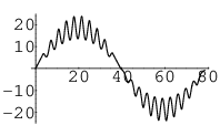
Tables 1, 2 and Figures 5-32 show results of our numerical computations.

Refer to caption
Refer to caption
Refer to caption
Refer to caption
Refer to caption
Refer to caption
Refer to caption
Refer to caption
Refer to caption
Refer to caption
Refer to caption
Refer to caption
Refer to caption
Refer to caption
Refer to caption
Figure 12. Eigenfunctions associated to the eigenvalues λ1,0\lambda_{1,0}, …, λ14,0\lambda_{14,0}, λ15,0=0\lambda_{15,0}=0 of the surface U8U_{8}.
Refer to caption
Refer to caption
Refer to caption
Refer to caption
Refer to caption
Refer to caption
Refer to caption
Refer to caption
Refer to caption
Refer to caption
Refer to caption
Refer to caption
Refer to caption
Refer to caption
Refer to caption
Refer to caption
Refer to caption
Refer to caption
Refer to caption
Figure 13. Eigenfunctions associated to the eigenvalues λ1,0\lambda_{1,0}, …, λ18,0\lambda_{18,0}, λ19,0=0\lambda_{19,0}=0 of the surface U9U_{9}.
Refer to caption
Refer to caption
Refer to caption
Refer to caption
Refer to caption
Refer to caption
Refer to caption
Refer to caption
Refer to caption
Refer to caption
Refer to caption
Figure 14. Eigenfunctions associated to the eigenvalues λ1,0\lambda_{1,0}, …, λ10,0\lambda_{10,0}, λ11,0=0\lambda_{11,0}=0 of the surface U10U_{10}.
Refer to caption
Refer to caption
Refer to caption
Refer to caption
Refer to caption
Refer to caption
Refer to caption
Refer to caption
Refer to caption
Refer to caption
Refer to caption
Refer to caption
Refer to caption
Refer to caption
Refer to caption
Figure 15. Eigenfunctions associated to the eigenvalues λ1,0\lambda_{1,0}, …, λ14,0\lambda_{14,0}, λ15,0=0\lambda_{15,0}=0 of the surface U11U_{11}.
Refer to caption
Refer to caption
Refer to caption
Refer to caption
Refer to caption
Refer to caption
Refer to caption
Refer to caption
Refer to caption
Refer to caption
Refer to caption
Refer to caption
Refer to caption
Refer to caption
Refer to caption
Refer to caption
Refer to caption
Refer to caption
Refer to caption
Refer to caption
Refer to caption
Refer to caption
Refer to caption
Figure 16. Eigenfunctions associated to the eigenvalues λ1,0\lambda_{1,0}, …, λ22,0\lambda_{22,0}, λ23,0=0\lambda_{23,0}=0 of the surface U12U_{12}.
Refer to caption
Refer to caption
Refer to caption
Refer to caption
Refer to caption
Refer to caption
Refer to caption
Refer to caption
Refer to caption
Refer to caption
Refer to caption
Refer to caption
Refer to caption
Refer to caption
Refer to caption
Figure 17. Eigenfunctions associated to the eigenvalues λ1,0\lambda_{1,0}, …, λ14,0\lambda_{14,0}, λ15,0=0\lambda_{15,0}=0 of the surface U13U_{13}.

References

  • [1] L. Barbosa, M. do Carmo and J. Eschenburg, Stability of hypersurfaces of constant mean curvature in Riemannian manifolds, Math. Z. 197 (1988), 123-138.
  • [2] P. Berard, Spectral Geometry: Direct and Inverse Problems, Lecture notes in Mathematics 1207 (1986).
  • [3] M. Berger, P. Gauduchon, E. Mazet, Le Spectre d’une Variete Riemannienne, Lecture Notes in Math. 194 (1971).
  • [4] S.-Y. Cheng, Eigenfunctions and nodal sets, Comment. Math. Helvetici 51 (1976), 43-55.
  • [5] R. Courant and D. Hilbert, Methods of mathematical physics, Volume I, Interscience publishers, Inc., New York, 1937.
  • [6] J. Diedonne, Foundation of Mathematical Analysis, Academic Press, 1960.
  • [7] P. Hartman, Ordinary differential equations, John Wiley and Sons, Inc., 1964.
  • [8] E. Hille, Lectures on ordinary differential equations, Addison-Wesley publishing company, 1969.
  • [9] W. Y. Hsiang, On generalization of theorems of A. D. Alexandrov and C. Delaunay on hypersurfaces of constant mean curvature, Duke Math. J. 49(3) (1982), 485-496.
  • [10] W. Y. Hsiang and W. C. Yu, A generalization of a theorem of Delaunay, J. Diff. Geom. 16 (1981), 161-177.
  • [11] H. B. Lawson Jr., Complete minimal surfaces in S3S^{3}, Ann. of Math. 92(2) (1970), 335-374.
  • [12] S. G. Mikhlin, Variational methods in mathematical physics, Pergamon Press (1964).
  • [13] W. Rossman, The Morse index of Wente tori, Geometria Dedicata 86 (2001), 129-151.
  • [14] W. Rossman, The first bifurcation point for Delaunay nodoids, J. Exp. Math. 14(3) (2005), 331-342.
  • [15] W. Rossman, Lower bounds for Morse index of constant mean curvature tori, Bull. London Math. Soc. 34 (2002), 599-609.
  • [16] W. Rossman and N. Sultana, Morse index of constant mean curvature tori of revolution in the 3-sphere, preprint, arXiv:math.DG/0605127.
  • [17] N. Schmitt, M. Kilian, S-P. Kobayashi, W. Rossman, Constant mean curvature surfaces with Delaunay ends in 33-dimensional space forms, to appear in J. London Math. Soc.
  • [18] N. Sultana, Explicit parametrization of Delaunay surfaces in space forms via loop group methods, Kobe Journal of Mathematics Vol. 22, No. 1-2 (2005).
  • [19] H. Urakawa, Geometry of Laplace-Beltrami operator on a complete Riemannian manifold, Progress on Diff. Geometry, Adv. Stud. Pure Math. 22 (1993), 347-406.
Refer to caption
Refer to caption
Refer to caption
Refer to caption
Refer to caption
Refer to caption
Refer to caption
Refer to caption
Refer to caption
Refer to caption
Refer to caption
Refer to caption
Refer to caption
Refer to caption
Refer to caption
Refer to caption
Refer to caption
Refer to caption
Refer to caption
Figure 18. Eigenfunctions associated to the eigenvalues λ1,0\lambda_{1,0}, …, λ18,0\lambda_{18,0}, λ19,0=0\lambda_{19,0}=0 of the surface U14U_{14}.
Refer to caption
Refer to caption
Refer to caption
Refer to caption
Refer to caption
Refer to caption
Refer to caption
Refer to caption
Refer to caption
Refer to caption
Refer to caption
Refer to caption
Refer to caption
Refer to caption
Refer to caption
Refer to caption
Refer to caption
Refer to caption
Refer to caption
Refer to caption
Refer to caption
Refer to caption
Refer to caption
Figure 19. Eigenfunctions associated to the eigenvalues λ1,0\lambda_{1,0}, …, λ22,0\lambda_{22,0}, λ23,0=0\lambda_{23,0}=0 of the surface U15U_{15}.
Refer to caption
Refer to caption
Refer to caption
Refer to caption
Refer to caption
Refer to caption
Refer to caption
Refer to caption
Refer to caption
Refer to caption
Refer to caption
Refer to caption
Refer to caption
Refer to caption
Refer to caption
Refer to caption
Refer to caption
Refer to caption
Refer to caption
Figure 20. Eigenfunctions associated to the eigenvalues λ1,0\lambda_{1,0}, …, λ18,0\lambda_{18,0}, λ19,0=0\lambda_{19,0}=0 of the surface U16U_{16}.
Refer to caption
Refer to caption
Refer to caption
Refer to caption
Refer to caption
Refer to caption
Refer to caption
Refer to caption
Refer to caption
Refer to caption
Refer to caption
Refer to caption
Refer to caption
Refer to caption
Refer to caption
Refer to caption
Refer to caption
Refer to caption
Refer to caption
Refer to caption
Refer to caption
Refer to caption
Refer to caption
Figure 21. Eigenfunctions associated to the eigenvalues λ1,0\lambda_{1,0}, …, λ22,0\lambda_{22,0}, λ23,0=0\lambda_{23,0}=0 of the surface U17U_{17}.
Refer to caption
Refer to caption
Refer to caption
Refer to caption
Refer to caption
Refer to caption
Refer to caption
Figure 22. Eigenfunctions associated to the eigenvalues λ1,0\lambda_{1,0}, …, λ6,0\lambda_{6,0}, λ7,0=0\lambda_{7,0}=0 of the surface N1N_{1}.
Refer to caption
Refer to caption
Refer to caption
Refer to caption
Refer to caption
Refer to caption
Refer to caption
Figure 23. Eigenfunctions associated to the eigenvalues λ1,0\lambda_{1,0}, …, λ6,0\lambda_{6,0}, λ7,0=0\lambda_{7,0}=0 of the surface N2N_{2}.
Refer to caption
Refer to caption
Refer to caption
Refer to caption
Refer to caption
Refer to caption
Refer to caption
Refer to caption
Refer to caption
Figure 24. Eigenfunctions associated to the eigenvalues λ1,0\lambda_{1,0}, …, λ8,0\lambda_{8,0}, λ9,0=0\lambda_{9,0}=0 of the surface N3N_{3}.
Refer to caption
Refer to caption
Refer to caption
Refer to caption
Refer to caption
Refer to caption
Refer to caption
Refer to caption
Refer to caption
Figure 25. Eigenfunctions associated to the eigenvalues λ1,0\lambda_{1,0}, …, λ8,0\lambda_{8,0}, λ9,0=0\lambda_{9,0}=0 of the surface N4N_{4}.
Refer to caption
Refer to caption
Refer to caption
Refer to caption
Refer to caption
Refer to caption
Refer to caption
Refer to caption
Refer to caption
Refer to caption
Refer to caption
Figure 26. Eigenfunctions associated to the eigenvalues λ1,0\lambda_{1,0}, …, λ10,0\lambda_{10,0}, λ11,0=0\lambda_{11,0}=0 of the surface N5N_{5}.
Refer to caption
Refer to caption
Refer to caption
Refer to caption
Refer to caption
Refer to caption
Refer to caption
Refer to caption
Refer to caption
Refer to caption
Refer to caption
Refer to caption
Refer to caption
Figure 27. Eigenfunctions associated to the eigenvalues λ1,0\lambda_{1,0}, …, λ12,0\lambda_{12,0}, λ13,0=0\lambda_{13,0}=0 of the surface N6N_{6}.
Refer to caption
Refer to caption
Refer to caption
Refer to caption
Refer to caption
Refer to caption
Refer to caption
Refer to caption
Refer to caption
Refer to caption
Refer to caption
Figure 28. Eigenfunctions associated to the eigenvalues λ1,0\lambda_{1,0}, …, λ10,0\lambda_{10,0}, λ11,0=0\lambda_{11,0}=0 of the surface N7N_{7}.
Refer to caption
Refer to caption
Refer to caption
Refer to caption
Refer to caption
Refer to caption
Refer to caption
Refer to caption
Refer to caption
Refer to caption
Refer to caption
Refer to caption
Refer to caption
Refer to caption
Refer to caption
Figure 29. Eigenfunctions associated to the eigenvalues λ1,0\lambda_{1,0}, …, λ14,0\lambda_{14,0}, λ15,0=0\lambda_{15,0}=0 of the surface N8N_{8}.
Refer to caption
Refer to caption
Refer to caption
Refer to caption
Refer to caption
Refer to caption
Refer to caption
Refer to caption
Refer to caption
Refer to caption
Refer to caption
Refer to caption
Refer to caption
Refer to caption
Refer to caption
Refer to caption
Refer to caption
Figure 30. Eigenfunctions associated to the eigenvalues λ1,0\lambda_{1,0}, …, λ16,0\lambda_{16,0}, λ17,0=0\lambda_{17,0}=0 of the surface N9N_{9}.
Refer to caption
Refer to caption
Refer to caption
Refer to caption
Refer to caption
Refer to caption
Refer to caption
Refer to caption
Refer to caption
Refer to caption
Refer to caption
Refer to caption
Refer to caption
Refer to caption
Refer to caption
Refer to caption
Refer to caption
Refer to caption
Refer to caption
Refer to caption
Refer to caption
Refer to caption
Refer to caption
Figure 31. Eigenfunctions associated to the eigenvalues λ1,0\lambda_{1,0}, …, λ22,0\lambda_{22,0}, λ23,0=0\lambda_{23,0}=0 of the surface N10N_{10}.
Refer to caption
Refer to caption
Refer to caption
Refer to caption
Refer to caption
Refer to caption
Refer to caption
Refer to caption
Refer to caption
Refer to caption
Refer to caption
Refer to caption
Refer to caption
Refer to caption
Refer to caption
Refer to caption
Refer to caption
Refer to caption
Refer to caption
Refer to caption
Refer to caption
Refer to caption
Refer to caption
Figure 32. Eigenfunctions associated to the eigenvalues λ1,0\lambda_{1,0}, …, λ22,0\lambda_{22,0}, λ23,0=0\lambda_{23,0}=0 of the surface N11N_{11}.