A Quasi-Newton Approach to
Nonsmooth Convex Optimization

Abstract

We extend the well-known BFGS quasi-Newton method and its limited-memory variant LBFGS to the optimization of nonsmooth convex objectives. This is done in a rigorous fashion by generalizing three components of BFGS to subdifferentials: The local quadratic model, the identification of a descent direction, and the Wolfe line search conditions. We apply the resulting subLBFGS algorithm to $L_{2}$-regularized risk minimization with the binary hinge loss. To extend our algorithm to the multiclass and multilabel settings we develop a new, efficient, exact line search algorithm. We prove its worst-case time complexity bounds, and show that it can also extend a recently developed bundle method to the multiclass and multilabel settings. We also apply the direction-finding component of our algorithm to $L_{1}$-regularized risk minimization with logistic loss. In all these contexts our methods perform comparable to or better than specialized state-of-the-art solvers on a number of publicly available datasets. Open source software implementing our algorithms is freely available for download.

1 Introduction

The BFGS quasi-Newton method (Nocedal and Wright, 1999) and its memory-limited LBFGS variant are widely regarded as the workhorses of smooth nonlinear optimization due to their combination of computational efficiency and good asymptotic convergence. Given a smooth objective function $J:\RR^{d}\rightarrow\RR$ and a current iterate $\bm{w}_{t}\in\RR^{d}$, BFGS forms a local quadratic model of $J$:

$$Q_{t}(\bm{p})~:=~J(\bm{w}_{t})+\half\bm{p}^{\top}\bm{B}_{t}^{-1}\bm{p}+\nabla J(\bm{w}_{t})^{\top}{\bm{p}},$$ (1)

where $\bm{B}_{t}\succ 0$ is a positive-definite estimate of the inverse Hessian of $J$, and $\nabla J$ denotes the gradient. Minimizing $Q_{t}(\bm{p})$ gives the quasi-Newton direction

$$\bm{p}_{t}:=-\bm{B}_{t}\nabla J(\bm{w}_{t}),$$ (2)

which is used for the parameter update:

$$\bm{w}_{t+1}=\bm{w}_{t}+\eta_{t}\bm{p}_{t}.$$ (3)

The step size $\eta_{t}>0$ is normally determined by a line search obeying the Wolfe conditions:

$$J(\bm{w}_{t+1})~\leq~J(\bm{w}_{t})+c_{1}\eta_{t} \nabla J(\bm{w}_{t})^{\top}\bm{p}_{t}\mbox{~~~~~~~~(sufficient decrease)}$$ (4)

$$\mbox{and~~~}\nabla J(\bm{w}_{t+1})^{\top}\bm{p}_{t}~\geq~c_{2} \nabla J(\bm{w}_{t})^{\top}\bm{p}_{t},\mbox{~~~~~~~(curvature)}$$ (5)

with $0<c_{1}<c_{2}<1$. The matrix $\bm{B}_{t}$ is then modified via the incremental rank-two update

$$\bm{B}_{t+1}=(\bm{I}-\rho_{t}\bm{s}_{t}\bm{y}_{t}^{\top})\bm{B}_{t}(\bm{I}-\rho_{t}\bm{y}_{t}\bm{s}_{t}^{\top})+\rho_{t}\bm{s}_{t}\bm{s}_{t}^{\top},$$ (6)

where $\bm{s}_{t}:=\bm{w}_{t+1}-\bm{w}_{t}$ and $\bm{y}_{t}:=\nabla J(\bm{w}_{t+1})-\nabla J(\bm{w}_{t})$ denote the most recent step along the optimization trajectory in parameter and gradient space, respectively, and $\rho_{t}:=(\bm{y}_{t}^{\top}\bm{s}_{t})^{-1}$. The BFGS update (6) enforces the secant equation $\bm{B}_{t+1}\bm{y}_{t}=\bm{s}_{t}$. Given a descent direction $\bm{p}_{t}$, the Wolfe conditions ensure that $(\forall t)~\bm{s}_{t}^{\top}\bm{y}_{t}>0$ and hence $\bm{B}_{0}\succ 0\implies(\forall t)~\bm{B}_{t}\succ 0$.

Limited-memory BFGS (LBFGS) is a variant of BFGS designed for solving large-scale optimization problems where the $O(d^{2})$ cost of storing and updating $\bm{B}_{t}$ would be prohibitively expensive. LBFGS approximates the quasi-Newton direction (2) directly from the last $m$ pairs of $\bm{s}_{t}$ and $\bm{y}_{t}$ via a matrix-free approach. This reduces the cost to $O(md)$ space and time per iteration, with $m$ freely chosen (Nocedal and Wright, 1999).

Smoothness of the objective function is essential for standard (L)BFGS because both the local quadratic model (1) and the Wolfe conditions (4, 5) require the existence of the gradient $\nabla J$ at every point. Even though nonsmooth convex functions are differentiable everywhere except on a set of Lebesgue measure zero (Hiriart-Urruty and Lemaréchal, 1993), in practice (L)BFGS often fails to converge on such problems (Lukšan and Vlček, 1999; Haarala, 2004). Various subgradient-based approaches, such as subgradient descent (Nedich and Bertsekas, 2000) or bundle methods (Joachims, 2006; Teo et al., 2007; Franc and Sonnenburg, 2008), are therefore preferred.

Although a convex function might not be differentiable everywhere, a subgradient always exists (Rockafellar, 1970). Let $\bm{w}$ be a point where a convex function $J$ is finite. Then a subgradient is the normal vector of any tangential supporting hyperplane of $J$ at $\bm{w}$. Formally, $\bm{g}$ is called a subgradient of $J$ at $\bm{w}$ if and only if (Rockafellar, 1970)

$$J(\bm{w}^{\prime})~\geq~J(\bm{w})+(\bm{w}^{\prime}-\bm{w})^{\top}\!\bm{g}\quad\forall\bm{w}^{\prime}.$$ (7)

The set of all subgradients at a point is called the subdifferential, and is denoted $\partial J(\bm{w})$. If this set is not empty then $J$ is said to be subdifferentiable at $\bm{w}$. If it contains exactly one element, i.e., $\partial J(\bm{w})=\{\nabla J(\bm{w})\}$, then $J$ is differentiable at $\bm{w}$. Figure 1 gives geometric intuition.

Figure 1: Geometric intuition of a subgradient. The dashed lines are tangential to the hinge function (solid blue line). The normal vectors to these lines are subgradients.

In this paper we systematically modify the standard (L)BFGS algorithm so as to make it amenable to subgradients. This results in sub(L)BFGS, a new subgradient quasi-Newton method which is applicable to many nonsmooth convex optimization problems. In particular, by exploiting knowledge about the subgradients of the binary hinge loss and its generalizations to the multiclass and multilabel settings we apply our algorithm to a variety of machine learning problems.

In the next section we describe our new algorithm generically, before we discuss its application to $L_{2}$-regularized risk minimization with the binary hinge loss in Section 3. We describe a new efficient algorithm to identify the subdifferentiable points of a one-dimensional pointwise maximum of linear functions in Section 4, then use it to develop an exact line search to extend our algorithm to the multiclass and multilabel settings in Section 5. Section 6 compares and contrasts our work with other recent efforts in this area. We report our experimental results on a number of public datasets in Section 7, and conclude with a discussion and outlook in Section 8.

2 Subgradient BFGS Method

We modify the standard BFGS algorithm to derive our new algorithm (subBFGS, Algorithm 1) for nonsmooth convex optimization. Our modifications can be grouped into three areas, which we elaborate on in turn: generalizing the local quadratic model, finding a descent direction, and finding a step size that obeys a subgradient reformulation of the Wolfe conditions.

Algorithm 1  Subgradient BFGS (subBFGS)

1:  Initialize: $t:=0,\bm{w}_{0}=\bm{0},\bm{B}_{0}=\bm{I}$

2:  Set direction-finding stopping tolerances $\epsilon,k_{\text{max}}\in\RR_{+}$

3:  Compute (sub)gradient $\bm{g}_{0}\in\partial J(\bm{w}_{0})$

4:  while not converged do

5:   $\bm{p}_{t}={\tt descentDirection}(\bm{g}_{t},\epsilon,k_{\text{max}})$ (Algorithm 2)

6:   if $\bm{p}_{t}=\text{failure}$ then

7:    return $\bm{w}_{t}$

8:   end if

9:   Find $\eta_{t}$ that obeys (16) (e.g. Algorithm 3 or 5)

10:   $\bm{s}_{t}=\eta_{t}\bm{p}_{t}$

11:   $\bm{w}_{t+1}=\bm{w}_{t}+\bm{s}_{t}$

12:   Compute (sub)gradient $\bm{g}_{t+1}\in\partial J(\bm{w}_{t+1})$ (choose an arbitrary subgradient    if $J$ is subdifferentiable at $\bm{w}_{t+1}$)

13:   $\bm{y}_{t}=\bm{g}_{t+1}-\bm{g}_{t}$

14:   Update $\bm{B}_{t+1}$ via (6)

15:   $t:=t+1$

16:  end while

2.1 Generalizing the Local Quadratic Model

Recall that BFGS assumes that the objective function $J$ is differentiable everywhere, so that at the current iterate $\bm{w}_{t}$ we can construct a local quadratic model (1) of $J(\bm{w}_{t})$. For a nonsmooth objective function, such a model becomes ambiguous at non-differentiable points (Figure 2, left). To resolve the ambiguity, we could simply replace the gradient $\nabla J(\bm{w}_{t})$ in (1) with an arbitrary subgradient $\bm{g}_{t}\in\partial J(\bm{w}_{t})$. However, as will be discussed later, the resulting quasi-Newton direction $\bm{p}_{t}:=-\bm{B}_{t}\bm{g}_{t}$ is not necessarily a descent direction. To address this fundamental modeling problem, we first generalize the local quadratic model (1) as follows:

$$Q_{t}(\bm{p})~:=~J(\bm{w}_{t})+M_{t}(\bm{p}),\mbox{~~where}$$

$$M_{t}(\bm{p})~:=~\half\bm{p}^{\top}\bm{B}_{t}^{-1}\bm{p}~+\!\!\!\sup_{\bm{g}\in\partial J(\bm{w}_{t})}\!\!\!\bm{g}^{\top}\bm{p}.$$ (8)

Note that where $J$ is differentiable, (8) reduces to the familiar BFGS quadratic model (1). At non-differentiable points, however, the model is no longer quadratic, as the supremum may be attained at different elements of $\partial J(\bm{w}_{t})$ for different directions $\bm{p}$. Instead it can be viewed as the tightest pseudo-quadratic fit to $J$ at $\bm{w}_{t}$ (Figure 2, right).

Figure 2: Left: Many possible quadratic models (dotted lines) for the objective (solid blue line) at a subdifferentiable point. Right: The tightest pseudo-quadratic fit (8) (bold red dashes); note that it is not a quadratic.

Ideally, we would like to minimize $Q_{t}(\bm{p})$, or equivalently $M_{t}(\bm{p})$, in (8) to obtain the best search direction,

$$\bm{p}^{*}:=\arginf_{\bm{p}\in\RR^{d}}M_{t}(\bm{p}).$$ (9)

This is generally intractable due to the presence of a supremum over the entire subdifferential set $\partial J(\bm{w}_{t})$. In many machine learning problems, however, the set $\partial J(\bm{w}_{t})$ has some special structure that simplifies calculation of the supremum in (8). In what follows, we develop an iteration that is guaranteed to find a quasi-Newton descent direction, assuming an oracle that supplies $\argsup_{\bm{g}\in\partial J(\bm{w}_{t})}\bm{g}^{\top}{\bm{p}}$ for a given direction $\bm{p}\in\RR^{d}$. Efficient oracles for this purpose can be derived for many machine learning settings; in this paper we provide such oracles for $L_{2}$-regularized risk minimization with binary hinge loss (Section 3.1), multiclass and multilabel hinge losses (Section 5), and $L_{1}$-regularized logistic loss (Section 7.3).

2.2 Finding a Descent Direction

A direction $\bm{p}_{t}$ is a descent direction if and only if ${\bm{g}}^{\top}\!\bm{p}_{t}<0~\forall{\bm{g}}\in\partial J(\bm{w}_{t})$ (Belloni, 2005), or equivalently

$$\sup_{{\bm{g}}\in\partial J(\bm{w}_{t})}\!\!\!{\bm{g}}^{\top}\bm{p}_{t}~<~0.$$ (10)

In particular, for a smooth convex function the quasi-Newton direction (2) is always a descent direction because $\nabla J(\bm{w}_{t})^{\top}\bm{p}_{t}=-\nabla J(\bm{w}_{t})^{\top}\bm{B}_{t}\nabla J(\bm{w}_{t})<0$ holds due to the positivity of $\bm{B}_{t}$.

For nonsmooth functions, however, the quasi-Newton direction $\bm{p}_{t}:=-\bm{B}_{t}\bm{g}_{t}$ for a given $\bm{g}_{t}\in\partial J(\bm{w}_{t})$ may not fulfill the descent condition (10), making it impossible to find a step that obeys the Wolfe conditions (4, 5), thus causing a failure of the line search. We now present an iterative approach to finding a quasi-Newton descent direction.

Algorithm 2  $\bm{p}_{t}={\tt descentDirection}(\bm{g}^{(1)},\epsilon,k_{\text{max}})$

1:  input (sub)gradient $\bm{g}^{(1)}\in\partial J(\bm{w}_{t})$, tolerance $\epsilon>0$, iteration limit $k_{\text{max}}>0$,           and an oracle to calculate $\argsup_{\bm{g}\in\partial J(\bm{w})}=\bm{g}^{\top}\bm{p}$ for any given $\bm{w}$ and $\bm{p}$

2:  output descent direction $\bm{p}_{t}$

3:  Initialize: $i=1,~\bar{\bm{g}}^{(1)}=\bm{g}^{(1)},~\bm{p}^{(1)}=-\bm{B}_{t}\bm{g}^{(1)}$

4:  $\bm{g}^{(2)}=\argsup_{\bm{g}\in\partial J(\bm{w}_{t})}\bm{g}^{\top}\bm{p}^{(1)}$

5:  $\epsilon^{(1)}:=\bm{p}^{(1)\top}\bm{g}^{(2)}-\bm{p}^{(1)\top}\bar{\bm{g}}^{(1)}$

6:  while $(\bm{g}^{(i+1)\top}\bm{p}^{(i)}>0$ or $\epsilon^{(i)}>\epsilon)$ and $i<k_{\text{max}}$ do

7:   $\mu^{*}:=\min\left[1,\frac{(\bar{\bm{g}}^{(i)}-\bm{g}^{(i+1)})^{\top}\bm{B}_{t}\bar{\bm{g}}^{(i)}}{(\bar{\bm{g}}^{(i)}-\bm{g}^{(i+1)})^{\top}\bm{B}_{t}(\bar{\bm{g}}^{(i)}-\bm{g}^{(i+1)})}\right]$ (cf. (104))

8:   $\bar{\bm{g}}^{(i+1)}=(1-\mu^{*})\bar{\bm{g}}^{(i)}+\mu^{*}\bm{g}^{(i+1)}$

9:   $\bm{p}^{(i+1)}=(1-\mu^{*})\bm{p}^{(i)}-\mu^{*}\bm{B}_{t}\bm{g}^{(i+1)}$

10:   $\bm{g}^{(i+2)}=\argsup_{\bm{g}\in\partial J(\bm{w}_{t})}\bm{g}^{\top}\bm{p}^{(i+1)}$

11:   $\epsilon^{(i+1)}:=\min_{j\leq(i+1)}\left[\bm{p}^{(j)\top}\bm{g}^{(j+1)}-\half(\bm{p}^{(j)\top}\bar{\bm{g}}^{(j)}+\bm{p}^{(i+1)\top}\bar{\bm{g}}^{(i+1)})\right]$

12:   $i:=i+1$

13:  end while

14:  if $\bm{g}^{(i+1)\top}\bm{p}^{(i)}>0$ then

15:   return failure;

16:  else

17:   return $\argmin_{j\leq i}M_{t}(\bm{p}^{(j)})$.

18:  end if

Inspired by bundle methods (Teo et al., 2007), we build the following convex lower bound on $M_{t}(\bm{p})$ at iteration $i$:

$$M_{t}^{(i)}(\bm{p})~:=~\half\bm{p}^{\top}\bm{B}_{t}^{-1}\bm{p}\,+\,\sup_{j\leq i}\bm{g}^{(j)\top}\bm{p},$$ (11)

where $i,j\in\NN$ and $\bm{g}^{(j)}\in\partial J(\bm{w}_{t})~\forall j\leq i$. Given a $\bm{p}^{(i)}\in\RR^{d}$ the lower bound (11) is successively tightened by computing

$$\bm{g}^{(i+1)} :=\argsup_{\bm{g}\in\partial J(\bm{w}_{t})}\bm{g}^{\top}\bm{p}^{(i)},$$ (12)

such that $M_{t}^{(i)}(\bm{p})\leq M_{t}^{(i+1)}(\bm{p})\leq M_{t}(\bm{p})~\forall\bm{p}\in\RR^{d}$. Here we set $\bm{g}^{(1)}\in\partial J(\bm{w}_{t})$ arbitrarily, and assume that $\bm{g}^{(i+1)}$ is provided by an oracle (e.g. as described in Section 3.1). To solve $\inf_{\bm{p}\in\RR^{d}}M_{t}^{(i)}(\bm{p})$, we rewrite it as a constrained optimization problem:

$$\inf_{\bm{p},\xi}\;\left(\half\bm{p}^{\top}\bm{B}_{t}^{-1}\bm{p}+\xi\right)\mbox{~~s.t.~~}\bm{g}^{(j)\top}\bm{p}\leq\xi~~\forall j\leq i.$$ (13)

This problem can be solved exactly via quadratic programming, but doing so may incur substantial computational expense. Instead we adopt an alternative approach (Algorithm 2) which does not solve $\inf_{\bm{p}\in\RR^{d}}M_{t}^{(i)}(\bm{p})$ to optimality. The key idea is to write the proposed descent direction at iteration $i+1$ as a convex combination of $\bm{p}^{(i)}$ and $-\bm{B}_{t}\bm{g}^{(i+1)}$. The optimal combination coefficient $\mu^{*}$ can be computed exactly (Line 7 of Algorithm 2) using an argument based on maximizing dual progress (Smola et al., 2007, see also). Finally, to derive an implementable stopping criterion, we define

$$\epsilon^{(i)}:=\min_{j\leq i}\left[\bm{p}^{(j)\top}\bm{g}^{(j+1)}-\half(\bm{p}^{(j)\top}\bar{\bm{g}}^{(j)}+\bm{p}^{(i)\top}\bar{\bm{g}}^{(i)})\right],$$ (14)

where $\bar{\bm{g}}^{(i)}$ is an aggregated subgradient (Line 8 of Algorithm 2) which lies in the convex hull of $\bm{g}^{(j)}\in\partial J(\bm{w}_{t})~\forall j\leq i$. $\epsilon^{(i)}$ is monotonically decreasing, and upper bounds the distance from the optimal value of the dual of $M_{t}(\bm{p})$, leading us to a practical stopping criterion (Line 6 of Algorithm 2) for our direction-finding procedure.

A detailed derivation of Algorithm 2 is given in Appendix A; in Appendix B we prove that it converges to an $\epsilon$ precision solution in $O(1/\epsilon)$ iterations.

2.3 Subgradient Line Search

Figure 3: Geometric interpretation of the subgradient Wolfe conditions (16). Solid disks are subdifferentiable points; the slopes of dashed lines are indicated.

Given the current iterate $\bm{w}_{t}$ and a search direction $\bm{p}_{t}$, the task of a line search is to find a step size $\eta>0$ which decreases the objective function along the line $\bm{w}_{t}+\eta\bm{p}_{t}$, i.e.,

$$\mini_{\eta}\Phi(\eta):=J(\bm{w}_{t}+\eta\bm{p}_{t}).$$ (15)

The sufficient decrease condition (4) is used in line search routines to enforce a sufficient decrease in the objective value; and the curvature condition excludes unnecessarily small step sizes (Nocedal and Wright, 1999). However, the original Wolfe conditions require the objective function to be smooth. To extend them to nonsmooth convex problems, we propose the following subgradient reformulation:

$$J(\bm{w}_{t+1})~\leq~J(\bm{w}_{t})~+~c_{1}\eta_{t} \sup_{\bm{g}\in\partial J(\bm{w}_{t})}\bm{g}^{\top}\bm{p}_{t}$$

$$\mbox{and~~~~}\sup_{\bm{g}^{\prime}\in\partial J(\bm{w}_{t+1})}\bm{g}^{\prime\top}\bm{p}_{t}~\geq~c_{2} \sup_{\bm{g}\in\partial J(\bm{w}_{t})}\bm{g}^{\top}\bm{p}_{t},$$ (16)

where $0<c_{1}<c_{2}<1$. Figure 3 illustrates how these conditions enforce acceptance of non-trivial step sizes that decrease the objective value. In Appendix C we formally show that for any given descent direction we can always find a positive step size that satisfies (16).

2.4 A Toy Example

Figure 4: Left: the nonsmooth convex function (17); optimization trajectory of BFGS with inexact line search (center) and subBFGS (right) on this function.

We present a simple example to illustrate the problems faced by BFGS when working with a nonsmooth objective function, and how subBFGS with exact line search overcomes these problems. Consider the problem of minimizing

$$f(x,y)=10\;|x|+|y|$$ (17)

with respect to $x$ and $y$. Clearly, $f(x,y)$ is convex but nonsmooth, with the minimum located at $(0,0)$ (Figure 4, left). It is subdifferentiable whenever $x$ or $y$ is zero: $\partial_{x}f(0,\cdot)=[-10,10]$ and $\partial_{y}f(\cdot,0)=[-1,1]$. We call such lines of subdifferentiability in parameter space hinges.

We can minimize (17) with the standard BFGS algorithm, employing a backtracking line search (Nocedal and Wright, 1999, Procedure 3.1) that starts with a step size that obeys the curvature condition (5), then exponentially decays it until both Wolfe conditions (4, 5) are satisfied. The curvature condition forces BFGS to jump across at least one hinge, thus ensuring that the gradient displacement vector $\bm{y}_{t}$ in (6) is non-zero; this prevents BFGS from diverging. Moreover, with such an inexact line search BFGS will generally not step on any hinges directly, thus avoiding (in an ad-hoc manner) the problem of non-differentiablility. Although this algorithm quickly decreases the objective from the starting point $(1,1)$, it is then slowed down by heavy oscillations around the optimum (Figure 4, center), caused by the utter mismatch between BFGS’ quadratic model and the actual function.

A generally sensible strategy to eliminate oscillations and improve convergence is to use an exact line search that finds the optimum along a given descent direction (cf. Section 3.2.1). However, this optimum will often lie on a hinge (as it does in our toy example), where the function is not differentiable. If an arbitrary subgradient is supplied instead, the BFGS update (6) can produce a search direction which is not a descent direction, causing the next line search to fail. In our toy example, standard BFGS with exact line search consistently fails after the first step, which takes it to the hinge at $x=0$.

Unlike standard BFGS, subBFGS can handle hinges and thus reap the benefits of an exact line search. As Figure 4 (right) shows, once the first iteration of subBFGS lands it on the hinge at $x=0$, its direction-finding routine (Algorithm 2) finds a descent direction for the next step. In fact, on this simple example Algorithm 2 yields a vector with zero $x$ component, which takes subBFGS straight to the optimum on the second step.

Although the local model (8) of subLBFGS is nonsmooth, it only incorporates those hinges present at the current location — all others are smoothly approximated by the quasi-Newton mechanism. Thus subBFGS relies on an exact line search to land it directly on a hinge if that is the optimal step, so as to incorporate that hinge into its local model.

2.5 Limited-Memory Subgradient BFGS (subLBFGS)

It is straightforward to implement an LBFGS variant of our subBFGS algorithm: We simply modify Algorithms 1 and 2 to compute all products between $\bm{B}_{t}$ and a vector by means of the standard LBFGS matrix-free scheme (Nocedal and Wright, 1999).

3 subBFGS for $L_{2}$-Regularized Binary Hinge Loss

Many machine learning algorithms can be viewed as minimizing the $L_{2}$-regularized risk

$$J(\bm{w})~:=~\frac{\lambda}{2}\|\bm{w}\|^{2}\,+\,\frac{1}{n}\sum_{i=1}^{n}l(\bm{x}_{i},z_{i},\bm{w}),$$ (18)

where $\bm{x}_{i}\in\Xcal\subseteq\RR^{d}$ are the training instances, $z_{i}\in\Zcal\subseteq\ZZ$ the corresponding labels, and the loss $l$ is a non-negative convex function of $\bm{w}$ which measures the discrepancy between $z_{i}$ and the predictions arising from using $\bm{w}$. A loss function commonly used for binary classification is the binary hinge loss

$$l(\bm{x},z,\bm{w})~:=~\max(0,1-z\,\bm{w}^{\top}\bm{x}),$$ (19)

where $z\in\{\pm 1\}$. $L_{2}$-regularized risk minimization with the binary hinge loss is a convex but nonsmooth optimization problem; in this section we show how subBFGS (Algorithm 1) can be applied to this problem.

Let $\Ecal$, $\Mcal$, and $\Wcal$ index the set of points which are in error, on the margin, and well-classified, respectively:

$$\Ecal :=\{i\in\{1,2,\ldots,n\}:1-z_{i}\bm{w}^{\top}\bm{x}_{i}>0\},$$

$$\Mcal :=\{i\in\{1,2,\ldots,n\}:1-z_{i}\bm{w}^{\top}\bm{x}_{i}=0\},$$ (20)

$$\Wcal :=\{i\in\{1,2,\ldots,n\}:1-z_{i}\bm{w}^{\top}\bm{x}_{i}<0\}.$$

Differentiating (18) after plugging in (19) then yields

$$\partial J(\bm{w}) ~=~\lambda\,\bm{w}-\frac{1}{n}\sum_{i=1}^{n}\beta_{i}z_{i}\bm{x}_{i}~=~\bar{\bm{w}}-\frac{1}{n}\sum_{i\in\Mcal}\beta_{i}z_{i}\bm{x}_{i},$$ (21)

$$\mbox{where~~~}\bar{\bm{w}} :=\lambda\,\bm{w}-\frac{1}{n}\sum_{i\in\Ecal}z_{i}\bm{x}_{i}\mbox{~~~and~~~}\beta_{i}:=\left\{\begin{array}[]{cllr}1&\mbox{if}&i\in\Ecal,\\ \left[0,1\right]&\mbox{if}&i\in\Mcal,\\ 0&\mbox{if}&i\in\Wcal.\end{array}\right.$$

3.1 Efficient Oracle for the Direction-Finding Method

Recall that our subBFGS algorithm requires an oracle that provides $\argsup_{\bm{g}\in\partial J(\bm{w}_{t})}\bm{g}^{\top}\bm{p}$ for a given direction $\bm{p}$. For $L_{2}$-regularized risk minimization with binary hinge loss we can implement such an oracle at a computational cost of $O(d\,|\Mcal_{t}|)$, where $d$ is the dimension of $\bm{p}$ and $|\Mcal_{t}|$ the number of current margin points, which is normally much less than $n$. Towards this end we use (21) to obtain

$$\sup_{\bm{g}\in\partial J(\bm{w}_{t})}\bm{g}^{\top}\bm{p}~~ =\sup_{\beta_{i},i\in\Mcal_{t}}\left(\bar{\bm{w}}_{t}-\frac{1}{n}\sum_{i\in\Mcal_{t}}\beta_{i}z_{i}\bm{x}_{i}\right)^{\!\!\top}\!\!\bm{p}$$

$$=~\bar{\bm{w}}_{t}^{\top}\bm{p}\,-\frac{1}{n}\sum_{i\in\Mcal_{t}}\inf_{\beta_{i}\in[0,1]}(\beta_{i}z_{i}\bm{x}_{i}^{\top}\bm{p}).$$ (25)

Since for a given $\bm{p}$ the first term of the right-hand side of (25) is a constant, the supremum is attained when we set $\beta_{i}~\forall i\in\Mcal_{t}$ via the following strategy:

$$\beta_{i}:=\begin{cases}0&\text{if~~}z_{i}\bm{x}_{i}^{\top}\bm{p}_{t}\,\geq\,0,\\ 1&\text{if~~}z_{i}\bm{x}_{i}^{\top}\bm{p}_{t}\,<\,0.\end{cases}$$ (26)

3.2 Implementing the Line Search

Figure 5: Left: Piecewise quadratic function $\Phi$ of step size $\eta$; solid disks in the zoomed inset are subdifferentiable points. Right: The subgradient of $\Phi(\eta)$ increases monotonically with $\eta$, and jumps discontinuously at subdifferentiable points.

The one-dimensional convex function $\Phi$ (15) (Figure 5, left) obtained by restricting (18) to a line can be evaluated efficiently. To see this, rewrite the objective function as

$$J(\bm{w})~:=~\frac{\lambda}{2}\,\|\bm{w}\|^{2}\,+~\frac{1}{n}\,\bm{1}^{\top}\!\max(\bm{0},~\bm{1}-\bm{z}\cdot\bm{X}\bm{w}),$$ (27)

where $\bm{0}$ and $\bm{1}$ are column vectors of zeros and ones, respectively, $\cdot$ denotes the Hadamard (component-wise) product, and $\bm{z}\in\RR^{n}$ collects correct labels corresponding to each row of data in $\bm{X}:=[\bm{x}_{1},\bm{x}_{2},\cdots,\bm{x}_{n}]^{\top}\in\RR^{n\times d}$. Given a search direction $\bm{p}$ at a point $\bm{w}$, this allows us to write

$$\Phi(\eta) ~:=~J(\bm{w}+\eta\bm{p})$$

$$~~=~\frac{\lambda}{2}\,\|\bm{w}\|^{2}+\,\lambda\,\eta\,\bm{w}^{\top}\bm{p}\,+\,\frac{\lambda\,\eta^{2}}{2}\,\|\bm{p}\|^{2}\,+~\frac{1}{n}\,\bm{1}^{\top}\max\left[0,~(\bm{1}-(\bm{f}+\eta\,\Delta\bm{f}))\right],$$ (28)

where $\bm{f}:=\bm{z}\cdot\bm{X}\bm{w}$ and $\Delta\bm{f}:=\bm{z}\cdot\bm{X}\bm{p}$. Differentiating (28) with respect to $\eta$ gives the subdifferential of $\Phi$:

$$\partial\Phi(\eta)=\lambda\bm{w}^{\top}\bm{p}+\eta\lambda\|\bm{p}\|^{2}-\frac{1}{n}\bm{\delta}(\eta)^{\top}\Delta\bm{f},$$ (29)

where $\bm{\delta}(\eta)$ is an indicator function that outputs a vector $[\delta_{1}(\eta),\delta_{2}(\eta),\cdots,\delta_{n}(\eta)]^{\top}$ with

$$\delta_{i}(\eta):=\left\{\begin{array}[]{cll}1&\text{if}&f_{i}+\eta\,\Delta f_{i}\,<\,1,\\ \left[0,1\right]&\text{if}&f_{i}+\eta\,\Delta f_{i}\,=\,1,\\ 0&\text{if}&f_{i}+\eta\,\Delta f_{i}\,>\,1.\end{array}\right.$$

We cache $\bm{f}$ and $\Delta\bm{f}$, expending $O(nd)$ computational effort and using $O(n)$ storage. We also cache the scalars $\frac{\lambda}{2}\|\bm{w}\|^{2}$, $\lambda\,\bm{w}^{\top}\bm{p}$, and $\frac{\lambda}{2}\|\bm{p}\|^{2}$, each of which requires $O(d)$ work. The evaluation of $\bm{1}-(\bm{f}+\eta\,\Delta\bm{f})$, $\bm{\delta}(\eta)$, their inner product, and inner product in the final term of (28) all take $O(n)$ effort. Given the cached terms, all other terms in (28) can be computed in constant time, thus reducing the cost of evaluating $\Phi(\eta)$ (resp. its subgradient) to $O(n)$. Furthermore, from (3.2) we see that $\Phi(\eta)$ is differentiable everywhere except at

$$\eta_{i}:=(1-f_{i})/\Delta f_{i}\mbox{~~with~~}\Delta f_{i}\neq 0,$$ (33)

where it becomes subdifferentiable. At these points an element of the indicator vector (3.2) changes from $0$ to $1$ or vice versa (causing the subgradient to jump, as shown in Figure 5, right); otherwise $\bm{\delta}(\eta)$ remains constant. Using this property of $\bm{\delta}(\eta)$, we can update the last term of (29) in constant time when passing a hinge point (Line 25 of Algorithm 3). We are now in a position to introduce an exact line search which takes advantage of this scheme.

3.2.1 Exact Line Search

Figure 6: Nonsmooth convex function $\Phi$ of step size $\eta$. Solid disks are subdifferentiable points; the optimal step $\eta^{*}$ either falls on such a point (left), or lies between two such points (right).

Given a direction $\bm{p}$, the exact line search finds the optimal step size $\eta^{*}:=\argmin_{\eta\geq 0}\Phi(\eta)$ that satisfies $0\in\partial\Phi(\eta^{*})$, or equivalently

$$\inf\partial\Phi(\eta^{*})\leq 0\leq\sup\partial\Phi(\eta^{*}).$$ (34)

Since Algorithm 2 gives a descent direction, the optimal step is always positive. To see this, we use the chain rule to write $\partial\Phi(\eta)=\{\bm{g}^{\top}\bm{p}:\bm{g}\in\partial J(\bm{w}+\eta\bm{p})\}$, and hence

$$\sup\partial\Phi(\eta)=\sup_{\bm{g}\in\partial J(\bm{w}+\eta\bm{p})}\bm{g}^{\top}\bm{p}.$$ (35)

The descent condition (10) implies that

$$\sup\partial\Phi(0)=\sup_{\bm{g}\in\partial J(\bm{w})}\bm{g}^{\top}\bm{p}<0.$$ (36)

For the piecewise quadratic function $\Phi(\eta)$ it is easy to prove that $\sup\partial\Phi(\eta)$ is monotonically increasing with $\eta$ (Hiriart-Urruty and Lemaréchal, 1993, Part I, VI.6, Proposition 6.1.1); hence, from (36) and (34) we have $\sup\partial\Phi(\eta^{*})>\sup\partial\Phi(0)\Rightarrow\eta^{*}>0$.

Using the monotonicity of $\sup\partial\Phi(\eta)$, our line search starts with $\eta=0$, and then walks through a sorted (in non-descending order) list of positive subdifferentiable points until it locates an interval $[\eta_{a},\eta_{b}]$ between two subdifferential points with $\sup\partial\Phi(\eta_{a})\leq 0$ and $\sup\partial\Phi(\eta_{b})\geq 0$. We now know that the optimal step size either coincides with $\eta_{b}$ (Figure 6, left), or lies in $(\eta_{a},\eta_{b})$ (Figure 6, right). It is easy to check whether $\eta^{*}=\eta_{b}$: simply check if $0\in\sup\partial\Phi(\eta_{b})$. If on the other hand $\eta^{*}$ lies in the smooth interval $(\eta_{a},\eta_{b})$, then setting (29) to zero gives

$$\eta^{*}=\frac{\bm{\delta}(\eta^{\prime})^{\top}\Delta\bm{f}/n-\lambda\,\bm{w}^{\top}\bm{p}}{\lambda\,\|\bm{p}\|^{2}},~~\eta^{\prime}\in(\eta_{a},\eta_{b}).$$ (37)

See Algorithm 3 for the detailed implementation.

Algorithm 3  Exact Line Search for $L_{2}$-Regularized Binary Hinge Loss

1:  input $\bm{w},\bm{p},\lambda,\bm{f},$ and $\Delta\bm{f}$ as in (28)

2:  output optimal step size

3:  $h=\lambda\|\bm{p}\|^{2},~j:=1$

4:  $\bm{\eta}:=[(\bm{1}-\bm{f})./\Delta\bm{f},0]$ (vector of subdifferentiable points & zero)

5:  $\bm{\pi}={\tt argsort}(\bm{\eta})$ (indices sorted by non-descending value of $\bm{\eta}$)

6:  while $\eta_{\pi_{j}}\leq 0$ do

7:   $j:=j+1$

8:  end while

9:  $\eta:=\eta_{\pi_{j}}/2$

10:  for $i:=1$ to $\bm{f}.{\tt size}$ do

11:    $\delta_{i}:=\left\{\begin{array}[]{rl}1&\text{if~~}f_{i}+\eta\,\Delta f_{i}<1\\ 0&\text{otherwise}\end{array}\right.$ (value of $\bm{\delta}(\eta)$ (3.2) for any $\eta\in(0,\eta_{\pi_{j}})$)

12:  end for

13:  $\varrho:=\bm{\delta}^{\top}\Delta\bm{f}/n-\lambda\bm{w}^{\top}\!\bm{p}$

14:  $\eta:=0,~\varrho^{\prime}:=0$

15:  $g:=-\varrho$ (value of $\sup\partial\Phi(0)$)

16:  while $g<0$ do

17:   $\varrho^{\prime}:=\varrho$

18:   if $j>\bm{\pi}.{\tt size}$ then

19:    $\eta:=\infty$ (no more subdifferentiable points)

20:    break

21:   else

22:    $\eta:=\eta_{\pi_{j}}$

23:   end if

24:   repeat

25:    $\varrho:=\left\{\begin{array}[]{rl@{\hspace{19ex}}r}\varrho-\Delta f_{\pi_{j}}/n&\text{if~~}\delta_{\pi_{j}}=1\hfil\hskip 81.8053pt&\text{(move to next subdifferentiable~}\\ \varrho+\Delta f_{\pi_{j}}/n&\text{otherwise}\hfil\hskip 81.8053pt&\text{point and update $\varrho$ accordingly)}\end{array}\right.$

26:    $j:=j+1$

27:   until $\eta_{\pi_{j}}\neq\eta_{\pi_{j-1}}$ and $j\leq\bm{\pi}.{\tt size}$

28:   $g:=\eta h-\varrho$ (value of $\sup\partial\Phi(\eta_{\pi_{j-1}})$)

29:  end while

30:  return $\min(\eta,~\varrho^{\prime}/h)$

4 Segmenting a Pointwise Maximum of 1-D Linear Functions

The line search of Algorithm 3 requires a vector $\bm{\eta}$ listing the subdifferentiable points along the line $\bm{w}+\eta\bm{p}$, and sorts it in non-descending order (Line 5). For an objective function like (18) whose nonsmooth component is just a sum of hinge losses (19), this vector is very easy to compute (Line 4 of Algorithm 3). In order to apply our line search approach to multiclass and multilabel losses, however, we must solve a more general problem: We need to efficiently find the subdifferentiable points of a one-dimensional piecewise linear function $\varrho:\RR\to\RR$ defined to be the pointwise maximum of $r$ lines:

$$\varrho(\eta)=\max_{1\leq p\leq r}(b_{p}+\eta\,a_{p}),$$ (38)

where $a_{p}$ and $b_{p}$ denote the slope and offset of the $p^{\rm th}$ line, respectively. Clearly $\varrho$ is convex since it is the pointwise maximum of linear functions (Boyd and Vandenberghe, 2004, section 3.2.3), cf. Figure 7(a). The difficulty here is that although $\varrho$ consists of at most $r$ line segments bounded by at most $r-1$ subdifferentiable points, there are $r(r-1)/2$ candidates for these points, namely all intersections between any two of the $r$ lines. A naive algorithm to find the subdifferentiable points of $\varrho$ would therefore take $O(r^{2})$ time. In what follows, however, we show how this can be done in just $O(r\log r)$ time. In Section 5 we will then use this technique (Algorithm 4) to perform efficient exact line search in the multiclass and multilabel settings.

Algorithm 4 Segmenting a Pointwise Maximum of 1-D Linear Functions

1:  input vectors $\bm{a}$ and $\bm{b}$ of slopes and offsets          lower bound $L$, upper bound $U$, with $0\leq L<U\leq\infty$

2:  output sorted stack of subdifferentiable points $\bm{\eta}$            and corresponding active line indices $\bm{\xi}$

3:  $\mathbf{y}:=\bm{b}+L\bm{a}$

4:  $\bm{\pi}:={\tt argsort}(-\mathbf{y})$ (indices sorted by non-ascending value of $\mathbf{y}$)

5:  $S.\mathrm{\tt push}~(L,\pi_{1})$ (initialize stack)

6:  for $q:=2\;\;\mathbf{to}\;\;\mathbf{y}.{\tt size}$ do

7:   while not $S.{\tt empty}$ do

8:    $(\eta,\xi):=S.{\tt top}$

9:    $\displaystyle\rule{0.0pt}{17.22217pt}\eta^{\prime}:=\frac{b_{\pi_{q}}-b_{\xi}}{\text{\raisebox{8.61108pt}{$a_{\xi}-a_{\pi_{q}}$}}}$ (intersection of two lines)

10:    if $L<\eta^{\prime}\leq\eta$ or ($\eta^{\prime}=L$ and $a_{\pi_{q}}>a_{\xi}$) then

11:     $S.{\tt pop}$ (cf. Figure 7(c))  

12:    else

13:     break

14:    end if

15:   end while

16:   if $L<\eta^{\prime}\leq U$ or ($\eta^{\prime}=L$ and $a_{\pi_{q}}>a_{\xi}$) then

17:    $S.{\tt push}~(\eta^{\prime},\pi_{q})$ (cf. Figure 7(b))  

18:   end if

19:  end for

20:  return $S$

We begin by specifying an interval $[L,U]~(0\leq L<U<\infty)$ in which to find the subdifferentiable points of $\varrho$, and set $\mathbf{y}:=\bm{b}+L\bm{a}$, where $\bm{a}=[a_{1},a_{2},\cdots,a_{r}]$ and $\bm{b}=[b_{1},b_{2},\cdots,b_{r}]$. In other words, $\mathbf{y}$ contains the intersections of the $r$ lines defining $\varrho(\eta)$ with the vertical line $\eta=L$. Let $\bm{\pi}$ denote the permutation that sorts $\mathbf{y}$ in non-ascending order, i.e., $p<q\implies y_{\pi_{p}}\geq y_{\pi_{q}}$, and let $\varrho^{(q)}$ be the function obtained by considering only the top $q\leq r$ lines at $\eta=L$, i.e., the first $q$ lines in $\bm{\pi}$:

$$\varrho^{(q)}(\eta)=\max_{1\leq p\leq q}(b_{\pi_{p}}+\eta\,a_{\pi_{p}}).$$ (39)

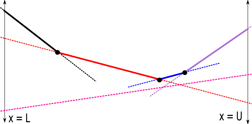
It is clear that $\varrho^{(r)}=\varrho$. Let $\bm{\eta}$ contain all $q^{\prime}\leq q-1$ subdifferentiable points of $\varrho^{(q)}$ in $[L,U]$ in ascending order, and $\bm{\xi}$ the indices of the corresponding active lines, i.e., the maximum in (39) is attained for line $\xi_{j-1}$ over the interval $[\eta_{j-1},\eta_{j}]$: $\xi_{j-1}:=\pi_{p^{*}}$, where $p^{*}=\argmax_{1\leq p\leq q}(b_{\pi_{p}}+\eta a_{\pi_{p}})\text{~for~}\eta\in[\eta_{j-1},\eta_{j}]$, and lines $\xi_{j-1}$ and $\xi_{j}$ intersect at $\eta_{j}$. Initially we set $\eta_{0}:=L$ and $\xi_{0}:=\pi_{1}$, the leftmost bold segment in Figure 7(a). Algorithm 4 goes through lines in $\bm{\pi}$ sequentially, and maintains a stack $S$ which at the end of the $q^{\rm th}$ iteration consists of the tuples $(\eta_{0},\xi_{0}),(\eta_{1},\xi_{1}),\ldots,(\eta_{q^{\prime}},\xi_{q^{\prime}})$ in order of ascending $\eta_{i}$, with $(\eta_{q^{\prime}},\xi_{q^{\prime}})$ at the top. After $r$ iterations $S$ contains a sorted list of all subdifferentiable points (and the corresponding active lines) of $\varrho=\varrho^{(r)}$ in $[L,U]$, as required by our line searches.

In iteration $q+1$ Algorithm 4 examines the intersection $\eta^{\prime}$ between lines $\xi_{q^{\prime}}$ and $\pi_{q+1}$: If $\eta^{\prime}>U$, line $\pi_{q+1}$ is irrelevant, and we proceed to the next iteration. If $\eta_{q^{\prime}}<\eta^{\prime}\leq U$ as in Figure 7(b), then line $\pi_{q+1}$ is becoming active at $\eta^{\prime}$, and we simply push $(\eta^{\prime}\!,\pi_{q+1})$ onto the stack. If $\eta^{\prime}\leq\eta_{q^{\prime}}$ as in Figure 7(c), on the other hand, then line $\pi_{q+1}$ dominates line $\xi_{q^{\prime}}$ over the interval $(\eta^{\prime}\!,\infty)$ and hence over $(\eta_{q^{\prime}},U]\subset(\eta^{\prime}\!,\infty)$, so we pop $(\eta_{q^{\prime}},\xi_{q^{\prime}})$ from the stack (deactivating line $\xi_{q^{\prime}}$), decrement $q^{\prime}\!$, and repeat the comparison.

(a) Pointwise maximum of lines

(b) Case 1

(c) Case 2

Figure 7: (a) Convex piecewise linear function defined as the maximum of 5 lines, but comprising only 4 active line segments (bold) separated by 3 subdifferentiable points (black dots). (b, c) Two cases encountered by our algorithm: (b) The new intersection (black cross) lies to the right of the previous one (red dot) and is therefore pushed onto the stack; (c) The new intersection lies to the left of the previous one. In this case the latter is popped from the stack, and a third intersection (blue square) is computed and pushed onto it.

Theorem 1.

The total running time of Algorithm 4 is $O(r\log r)$.

Proof.

Computing intersections of lines as well as pushing and popping from the stack require $O(1)$ time. Each of the $r$ lines can be pushed onto and popped from the stack at most once; amortized over $r$ iterations the running time is therefore $O(r)$. The time complexity of Algorithm 4 is thus dominated by the initial sorting of $\mathbf{y}$ (i.e., the computation of $\bm{\pi}$), which takes $O(r\log r)$ time. ∎

5 subBFGS for Multiclass and Multilabel Hinge Losses

We now use the algorithm developed in Section 4 to generalize the subBFGS method of Section 3 to the multiclass and multilabel settings with finite label set $\Zcal$. We assume that given an instance $\bm{x}$ our classifier predicts the label $z^{*}=\argmax_{z\in\Zcal}f(\bm{w},\bm{x},z)$, where $f$ is a linear function of $\bm{w}$, i.e., $f(\bm{w},\bm{x},z)={\bm{w}}^{\!\top}\!{\phi(\bm{x},z)}$ for some feature map $\phi(\bm{x},z)$.

5.1 Multiclass Hinge Loss

A variety of multiclass hinge losses have been proposed in the literature that generalize the binary hinge loss and enforce a margin of separation between the true label $z_{i}$ and every other label. We focus on the following rather general variant (Taskar et al., 2004):

$$l(\bm{x}_{i},z_{i},\bm{w})~:=~\max_{z\in\Zcal}\,[\Delta(z,z_{i})+f(\bm{w},\bm{x}_{i},z)-f(\bm{w},\bm{x}_{i},z_{i})],$$ (40)

where $\Delta(z,z_{i})\geq 0$ is the label loss specifying the margin required between labels $z$ and $z_{i}$. For instance, a uniform margin of separation is achieved by setting $\Delta(z,z^{\prime}):=\tau>0~\forall z\neq z^{\prime}$ (Crammer and Singer, 2003a). By requiring that $\forall z\in\Zcal:\Delta(z,z)=0$ we ensure that (40) always remains non-negative. Adapting (18) to the multiclass hinge loss (40) we obtain

$$J(\bm{w})~:=~\frac{\lambda}{2}\|\bm{w}\|^{2}+\frac{1}{n}\sum_{i=1}^{n}\max_{z\in\Zcal}\,[\Delta(z,z_{i})+f(\bm{w},\bm{x}_{i},z)-f(\bm{w},\bm{x}_{i},z_{i})].$$ (41)

For a given $\bm{w}$, consider the set

$$\Zcal_{i}^{*}:=\,\argmax_{z\in\Zcal}[\Delta(z,z_{i})+f(\bm{w},\bm{x}_{i},z)-f(\bm{w},\bm{x}_{i},z_{i})]$$ (42)

of maximum-loss labels (possibly more than one) for the $i^{\rm th}$ training instance. Since $f(\bm{w},\bm{x},z)={\bm{w}}^{\!\top}\!{\phi(\bm{x},z)}$, the subdifferential of (41) can then be written as

$$\partial J(\bm{w}) ~=~\lambda\bm{w}+\frac{1}{n}\sum_{i=1}^{n}\sum_{z\in\Zcal}\beta_{i,z}\,\phi(\bm{x}_{i},z)$$ (43)

$$\text{with~~~}\beta_{i,z} ~=~\left\{\begin{array}[]{rl}[0,1]&\text{if~}z\in\Zcal_{i}^{*}\\ 0&\text{otherwise}\end{array}\right\}\,-\,\delta_{z,z_{i}}\text{~~s.t.~~}\sum_{z\in\Zcal}\beta_{i,z}=0,$$

where $\delta$ is the Kronecker delta: $\delta_{a,b}=1$ if $a=b$, and 0 otherwise.

5.2 Efficient Multiclass Direction-Finding Oracle

For $L_{2}$-regularized risk minimization with multiclass hinge loss, we can use a similar scheme as described in Section 3.1 to implement an efficient oracle that provides $\argsup_{\bm{g}\in\partial J(\bm{w})}\bm{g}^{\!\top}\!\bm{p}$ for the direction-finding procedure (Algorithm 2). Using (43), we can write

$$\sup_{\bm{g}\in\partial J(\bm{w})}\!\bm{g}^{\!\top}\!\bm{p}~=~\lambda\bm{w}^{\!\top}\!\bm{p}\,+\,\frac{1}{n}\sum^{n}_{i=1}\,\sum_{z\in\Zcal}\,\sup_{\beta_{i,z}}\left(\beta_{i,z}\,\phi(\bm{x}_{i},z)^{\!\top}\!\bm{p}\right).$$ (46)

This supremum is attained when we pick, from the choices offered by (5.1),

$$\beta_{i,z}\,:=\,\delta_{z,z_{i}^{*}}-\delta_{z,z_{i}},\text{~~where~~~}z_{i}^{*}\,:=\,\argmax_{z\in\Zcal_{i}^{*}}\phi(\bm{x}_{i},z)^{\!\top}\!\bm{p}.$$ (47)

5.3 Implementing the Multiclass Line Search

Let $\Phi(\eta):=J(\bm{w}+\eta\bm{p})$ be the one-dimensional convex function obtained by restricting (41) to a line along direction $\bm{p}$. Letting $\varrho_{i}(\eta):=l(\bm{x}_{i},z_{i},\bm{w}+\eta\bm{p})$ we can write

$$\Phi(\eta)~=~\frac{\lambda}{2}\|\bm{w}\|^{2}+\,\lambda\eta{\bm{w}}^{\!\top}\!{\bm{p}}\,+\frac{\lambda\eta^{2}}{2}\|\bm{p}\|^{2}\,+\,\frac{1}{n}\sum_{i=1}^{n}\varrho_{i}(\eta).$$ (48)

Each $\varrho_{i}(\eta)$ is a piecewise linear convex function. To see this, observe that $f(\bm{w}+\eta\bm{p},\bm{x},z):={(\bm{w}+\eta\bm{p})}^{\!\top}\!{\phi(\bm{x},z)}=f(\bm{w},\bm{x},z)+\eta f(\bm{p},\bm{x},z)$ and hence

$$\varrho_{i}(\eta)\,:=\,\max_{z\in\Zcal}\;[\underbrace{\Delta(z,z_{i})+f(\bm{w},\bm{x}_{i},z)-f(\bm{w},\bm{x}_{i},z_{i})}_{=:\>b_{z}^{(i)}}\,+~\eta\underbrace{(f(\bm{p},\bm{x}_{i},z)-f(\bm{p},\bm{x}_{i},z_{i}))}_{=:\>a_{z}^{(i)}}],$$ (49)

which has the functional form of (38) with $r=|\!\Zcal\!|$. Algorithm 4 can therefore be used to compute a sorted vector $\bm{\eta}^{(i)}$ of all subdifferentiable points of $\varrho_{i}(\eta)$ and corresponding active lines $\bm{\xi}^{(i)}\!$ in the interval $[0,\infty)$ in $O(|\!\Zcal\!|\log|\!\Zcal\!|)$ time. With some abuse of notation, we now have

$$\eta\in[\eta_{j}^{(i)},\eta_{j+1}^{(i)}]~\implies~\varrho_{i}(\eta)\,=\,b_{\xi_{j}^{(i)}}+\,\eta\,a_{\xi_{j}^{(i)}}.$$ (50)

The first three terms of (48) are constant, linear, and quadratic (with non-negative coefficient) in $\eta$, respectively. The remaining sum of piecewise linear convex functions $\varrho_{i}(\eta)$ is also piecewise linear and convex, and so $\Phi(\eta)$ is a piecewise quadratic convex function.

5.3.1 Exact Multiclass Line Search

Our exact line search employs a similar two-stage strategy as discussed in Section 3.2.1 for locating its minimum $\eta^{*}:=\argmin_{\eta>0}\Phi(\eta)$: We first find the first subdifferentiable point $\check{\eta}$ past the minimum, then locate $\eta^{*}$ within the differentiable region to its left. We precompute and cache a vector $\bm{a}^{(i)}$ of all the slopes $a_{z}^{(i)}$ (offsets $b_{z}^{(i)}\!$ are not needed), the subdifferentiable points $\bm{\eta}^{(i)}$ (sorted in ascending order via Algorithm 4), and the corresponding indices $\bm{\xi}^{(i)}$ of active lines of $\varrho_{i}$ for all training instances $i$, as well as $\|\bm{w}\|^{2}\!$, ${\bm{w}}^{\!\top}\!{\bm{p}}$, and $\lambda\|\bm{p}\|^{2}\!$.

Algorithm 5 Exact Line Search for $L_{2}$-Regularized Multiclass Hinge Loss

1:  input base point $\bm{w}$, descent direction $\bm{p}$, regularization parameter $\lambda$, vector $\bm{a}$ of          all slopes as defined in (49), for each training instance $i$: sorted stack $S_{i}$ of          subdifferentiable points and active lines as produced by Algorithm 4

2:  output optimal step size

3:  $\bm{a}:=\bm{a}/n,~h:=\lambda\|\bm{p}\|^{2}$

4:  $\varrho:=\lambda{\bm{w}}^{\!\top}\!{\bm{p}}$

5:  for $i:=1$ to $n$ do

6:   while not $S_{i}.{\tt empty}$ do

7:    $R_{i}.{\tt push}~S_{i}.{\tt pop}$ (reverse the stacks)  

8:   end while

9:   $(\cdot,\xi_{i}):=R_{i}.{\tt pop}$

10:   $\varrho:=\varrho+a_{\xi_{i}}$

11:  end for

12:  $\eta:=0,~\varrho^{\prime}=0$

13:  $g:=\varrho$ (value of $\sup\partial\Phi(0)$)

14:  while $g<0$ do

15:   $\varrho^{\prime}:=\varrho$

16:   if $\forall i:R_{i}.{\tt empty}$ then

17:    $\eta:=\infty$ (no more subdifferentiable points)

18:    break

19:   end if

20:   $\Ical:=\argmin_{1\leq i\leq n}~\eta^{\prime}:~(\eta^{\prime},\cdot)=R_{i}.{\tt top}$ (find the next subdifferentiable point)

21:   $\varrho:=\varrho-\sum_{i\in\Ical}a_{\xi_{i}}$

22:   $\Xi:=\{\xi_{i}:(\eta,\xi_{i}\!):=R_{i}.{\tt pop},~~i\in\Ical\}$

23:   $\varrho:=\varrho+\sum_{\xi_{i}\in\Xi}a_{\xi_{i}}$

24:   $g:=\varrho\!+\eta\,h$ (value of $\sup\partial\Phi(\eta)$)  

25:  end while

26:  return $\min(\eta,\,-\varrho^{\prime}\!/h)$

Since $\Phi(\eta)$ is convex, any point $\eta<\eta^{*}$ cannot have a non-negative subgradient. The first subdifferentiable point $\check{\eta}\geq\eta^{*}$ therefore obeys

$$\check{\eta} ~:=~\min\eta\in\{\bm{\eta}^{(i)}\!,\,i=1,2,\ldots,n\}:\eta\geq\eta^{*}$$ (51)

$$~~=~\min\eta\in\{\bm{\eta}^{(i)}\!,\,i=1,2,\ldots,n\}:\sup\,\partial\,\Phi(\eta)\geq 0.$$ (52)

We find $\check{\eta}$ via a simple linear search: Starting from $\eta=0$, we walk from one subdifferentiable point to the next until $\sup\,\partial\,\Phi(\eta)\geq 0$. To perform this walk efficiently, define a vector $\bm{\psi}\in\NN^{n}$ of indices into the sorted vector $\bm{\eta}^{(i)}$ resp. $\bm{\xi}^{(i)}$; initially $\bm{\psi}:=\bm{0}$, indicating that $(\forall i)~\eta_{0}^{(i)}=0$. Given the current index vector $\bm{\psi}$, the next subdifferentiable point is then

$$\eta^{\prime}:=\eta_{(\psi_{i^{\prime}}+1)}^{(i^{\prime})},\text{~~where~~}i^{\prime}=\argmin_{1\leq i\leq n}\eta_{(\psi_{i}+1)}^{(i)};$$ (53)

the step is completed by incrementing $\psi_{i^{\prime}}$, i.e., $\psi_{i^{\prime}}:=\psi_{i^{\prime}}+1$, so as to remove $\eta_{\psi_{i^{\prime}}}^{(i^{\prime})}$ from future consideration. Note that computing the $\argmin$ in (53) takes $O(\log n)$ time (e.g. using a priority queue). Inserting (50) into (48) and differentiating, we find that

$$\sup\,\partial\,\Phi(\eta^{\prime})~=~\lambda{\bm{w}}^{\!\top}\!{\bm{p}}+\lambda\eta^{\prime}\|\bm{p}\|^{2}+\frac{1}{n}\sum_{i=1}^{n}a_{\xi_{\psi_{i}}^{(i)}}.$$ (54)

The key observation here is that after the initial calculation of $\sup\partial\Phi(0)=\lambda{\bm{w}}^{\!\top}\!{\bm{p}}+\frac{1}{n}\sum_{i=1}^{n}a_{\xi_{0}^{(i)}}$ for $\eta=0$, the sum in (54) can be updated incrementally in constant time through the addition of $a_{\xi_{\psi_{i^{\prime}}}^{(i^{\prime})}}-a_{\xi_{(\psi_{i^{\prime}}-1)}^{(i^{\prime})}}\!$.

Suppose we find $\check{\eta}=\eta_{\psi_{i^{\prime}}}^{(i^{\prime})}$ for some $i^{\prime}$. We then know that the minimum $\eta^{*}$ is either equal to $\check{\eta}$ (Figure 6, left), or found within the quadratic segment immediately to its left (Figure 6, right). We thus decrement $\psi_{i^{\prime}}$ (i.e., take one step back) so as to index the segment in question, set the right-hand side of (54) to zero, and solve for $\eta^{\prime}$ to obtain

$$\eta^{*}~=~\min\!\left(\check{\eta},~~\frac{\lambda{\bm{w}}^{\!\top}\!{\bm{p}}+\frac{1}{n}\sum^{n}_{i=1}a_{\xi_{\psi_{i}}^{(i)}}}{-\lambda\|\bm{p}\|^{2}}\right).$$ (55)

This only takes constant time: We have cached ${\bm{w}}^{\!\top}\!{\bm{p}}$ and $\lambda\|\bm{p}\|^{2}$, and the sum in (55) can be obtained incrementally by adding $a_{\xi_{\psi_{i^{\prime}}}^{(i^{\prime})}}-a_{\xi_{(\psi_{i^{\prime}}+1)}^{(i^{\prime})}}\!$ to its last value in (54).

To locate $\check{\eta}$ we have to walk at most $O(n|\!\Zcal\!|)$ steps, each requiring $O(\log n)$ computation. Given $\check{\eta}$, the exact minimum $\eta^{*}$ can be obtained in $O(1)$. Including the preprocessing cost (for invoking Algorithm 4), our exact multiclass line search therefore takes $O(n|\!\Zcal\!|(\log n+\log|\!\Zcal\!|))$ time in the worst case. Algorithm 5 provides an implementation which instead of an index vector $\bm{\psi}$ directly uses the sorted stacks of subdifferentiable points and active lines produced by Algorithm 4. (The cost of reversing those stacks in Lines 6–8 of Algorithm 5 can easily be avoided through the use of double-ended queues.)

5.4 Multilabel Hinge Loss

Recently, there has been interest in extending the concept of the hinge loss to multilabel problems. Multilabel problems generalize the multiclass setting in that each training instance $\bm{x}_{i}$ is associated with a set of labels $\Zcal_{i}\subseteq\Zcal$ (Crammer and Singer, 2003b). For a uniform margin of separation $\tau$, a hinge loss can be defined in this setting as follows:

$$l(\bm{x}_{i},\Zcal_{i},\bm{w})\,:=\,\max[\,0,~\tau+\max_{z^{\prime}\notin\Zcal_{i}}f(\bm{w},\bm{x}_{i},z^{\prime})-\min_{z\in\Zcal_{i}}f(\bm{w},\bm{x}_{i},z)].$$ (56)

We can generalize this to a not necessarily uniform label loss $\Delta(z^{\prime},z)\geq 0$ as follows:

$$l(\bm{x}_{i},\Zcal_{i},\bm{w})\,:=\,\max_{\begin{subarray}{c}(z,z^{\prime}):\>z\in\Zcal_{i}\\ z^{\prime}\notin\,\Zcal_{i}\!\backslash\{z\}\end{subarray}}[\Delta(z^{\prime},z)+f(\bm{w},\bm{x}_{i},z^{\prime})-f(\bm{w},\bm{x}_{i},z)],$$ (57)

where as before we require that $\Delta(z,z)=0~\forall z\in\Zcal$, so that by explicitly allowing $z^{\prime}=z$ we can ensure that (57) remains non-negative. For a uniform margin $\Delta(z^{\prime},z)=\tau~\forall z^{\prime}\neq z$ our multilabel hinge loss (57) reduces to the decoupled version (56), which in turn reduces to the multiclass hinge loss (40) if $\Zcal_{i}:=\{z_{i}\}$ for all $i$.

For a given $\bm{w}$, let

$$\Zcal_{i}^{*}:=\argmax_{\begin{subarray}{c}(z,z^{\prime}):\>z\in\Zcal_{i}\\ z^{\prime}\notin\,\Zcal_{i}\!\backslash\{z\}\end{subarray}}[\Delta(z^{\prime},z)+f(\bm{w},\bm{x}_{i},z^{\prime})-f(\bm{w},\bm{x}_{i},z)]$$ (58)

be the set of worst label pairs (possibly more than one) for the $i^{\rm th}$ training instance. The subdifferential of the multilabel analogue of the $L_{2}$-regularized multiclass objective (41) can then be written just as in (43), with coefficients

$$\beta_{i,z}:=\!\!\!\!\!\sum_{z^{\prime}:\,(z^{\prime}\!,z)\in\Zcal_{i}^{*}}\!\!\!\!\!\gamma^{(i)}_{z^{\prime}\!,z}~-\!\!\!\!\!\sum_{z^{\prime}:\,(z,z^{\prime})\in\Zcal_{i}^{*}}\!\!\!\!\!\gamma^{(i)}_{z,z^{\prime}}\,,\text{~~where~~~}(\forall i)\!\!\sum_{(z,z^{\prime})\in\Zcal_{i}^{*}}\!\!\!\gamma^{(i)}_{z,z^{\prime}}\,=\,1\mbox{~~and~~}\gamma^{(i)}_{z,z^{\prime}}\geq 0.$$ (59)

Now let $(z_{i},z^{\prime}_{i}):=\argmax_{(z,z^{\prime})\in\Zcal_{i}^{*}}[\phi(\bm{x}_{i},z^{\prime})-\phi(\bm{x}_{i},z)]^{\top}\!\bm{p}$ be a single steepest worst label pair in direction $\bm{p}$. We obtain $\argsup_{\bm{g}\in\partial J(\bm{w})}\bm{g}^{\top}\bm{p}$ for our direction-finding procedure by picking, from the choices offered by (59), $\gamma^{{}_{(i)}}_{z,z^{\prime}}:=\delta_{z,z_{i}}\delta_{z^{\prime}\!,z^{\prime}_{i}}$.

Finally, the line search we described in Section 5.3 for the multiclass hinge loss can be extended in a straightforward manner to our multilabel setting. The only caveat is that now $\varrho_{i}(\eta):=l(\bm{x}_{i},\Zcal_{i},\bm{w}+\eta\bm{p})$ must be written as

$$\varrho_{i}(\eta)\,:=\!\!\max_{\begin{subarray}{c}(z,z^{\prime}):\>z\in\Zcal_{i}\\ z^{\prime}\notin\,\Zcal_{i}\!\backslash\{z\}\end{subarray}}[\underbrace{\Delta(z^{\prime},z)+f(\bm{w},\bm{x}_{i},z^{\prime})-f(\bm{w},\bm{x}_{i},z)}_{=:\>b^{(i)}_{z,z^{\prime}}}+\,\eta\underbrace{(f(\bm{p},\bm{x}_{i},z^{\prime})-f(\bm{p},\bm{x}_{i},z))}_{=:\>a^{(i)}_{z,z^{\prime}}}],\>$$ (60)

which in the worst case could be the piecewise maximum of $O(|\!\Zcal\!|^{2})$ lines, thus increasing the overall complexity of the line search. In practice the set of true labels $\Zcal_{i}$ is usually small, typically of size 2 or 3 (e.g., Crammer and Singer, 2003b, Figure 3). As long as $\forall i:|\!\Zcal_{i}\!|=O(1)$, our complexity estimates of Section 5.3.1 still apply.

6 Related Work

We discuss related work in two areas: Nonsmooth convex optimization, and the problem of segmenting the pointwise maximum of a set of one-dimensional linear functions.

6.1 Nonsmooth Convex Optimization

There are four main approaches to nonsmooth convex optimization: Quasi-Newton methods, bundle methods, stochastic dual methods, and smooth approximation. We discuss each of these briefly and compare and contrast our work with the state of the art.

6.1.1 Nonsmooth Quasi-Newton Methods

These methods try to find a descent quasi-Newton direction at every iteration, and invoke a line search to minimize the one-dimensional convex function along that direction. We note that the line search routines we describe in Sections 3–5 are applicable to all such methods. An example of this class of algorithms is the work of Lukšan and Vlček (1999), who propose an extension of BFGS to nonsmooth convex problems. Their algorithm samples (sub)gradients around non-differentiable points in order to obtain a descent direction. In many machine learning problems evaluating the objective function and its (sub)gradient is very expensive, making such an approach inefficient. In contrast, given a current iterate $\bm{w}_{t}$, our direction-finding routine (Algorithm 2) samples subgradients from the set $\partial J(\bm{w}_{t})$ via the oracle. Since this avoids the cost of explicitly evaluating new (sub)gradients, it is computationally more efficient.

Recently, Andrew and Gao (2007) introduced a variant of LBFGS, the Orthant-Wise Limited-memory Quasi-Newton (OWL-QN) algorithm, suitable for optimizing $L_{1}$-regularized log-linear models:

$$J(\bm{w}):=\lambda\|\bm{w}\|_{1}+\underbrace{\frac{1}{n}\sum_{i=1}^{n}\ln(1+e^{-z_{i}{\bm{w}}^{\!\top}\!{\bm{x}_{i}}})}_{\text{logistic loss}},$$ (61)

where the logistic loss is smooth, but the regularizer is only subdifferentiable at points where $\bm{w}$ has zero elements. From the optimization viewpoint this objective is very similar to the $L_{2}$-regularized hinge loss; the direction finding and line search methods that we discussed in Sections 2.2 and 2.3, respectively, can be applied to this problem with slight modifications.

OWL-QN is based on the observation that the $L_{1}$ regularizer is linear within any given orthant. Therefore, it maintains an approximation $\bm{B}^{\text{ow}}$ to the inverse Hessian of the logistic loss, and uses an efficient scheme to select orthants for optimization. In fact, its success greatly depends on its direction-finding subroutine, which demands a specially chosen subgradient $\bm{g}^{\text{ow}}$ (Andrew and Gao, 2007, Equation 4) to produce the quasi-Newton direction, $\bm{p}^{\text{ow}}=\pi(\bm{p},\bm{g}^{\text{ow}})$, where $\bm{p}:=-\bm{B}^{\text{ow}}\bm{g}^{\text{ow}}$ and the projection $\pi$ returns a search direction by setting the $i^{\text{th}}$ element of $\bm{p}$ to zero whenever $p_{i}g^{\text{ow}}_{i}>0$. As shown in Section 7.3, the direction-finding subroutine of OWL-QN can be replaced by our Algorithm 2, which makes OWL-QN more robust to the choice of subgradients.

6.1.2 Bundle Methods

Bundle method solvers (Hiriart-Urruty and Lemaréchal, 1993) use past (sub)gradients to build a model of the objective function. The (sub)gradients are used to lower-bound the objective by a piecewise linear function which is minimized to obtain the next iterate. This fundamentally differs from the BFGS approach of using past gradients to approximate the (inverse) Hessian, hence building a quadratic model of the objective function.

Bundle methods have recently been adapted to the machine learning context, where they are known as SVMStruct (Tsochantaridis et al., 2005) resp. BMRM (Smola et al., 2007). One notable feature of these variants is that they do not employ a line search. This is justified by noting that a line search involves computing the value of the objective function multiple times, a potentially expensive operation.

Franc and Sonnenburg (2008) speed up the convergence of SVMStruct for the $L_{2}$-regularized binary hinge loss. The main idea of their optimized cutting plane algorithm, OCAS, is to perform a line search along the line connecting two successive iterates of a bundle method solver. Although developed independently, their line search is very similar to the method we describe in Section 3.2.1.

6.1.3 Stochastic Dual Methods

Distinct from the above two classes of primal algorithms are methods which work in the dual domain. A prominent member of this class is the LaRank algorithm of Bordes et al. (2007), which achieves state-of-the-art results on multiclass classification problems. While dual algorithms are very competitive on clean datasets, they tend to be slow on noisy datasets. Furthermore, because of their stochastic nature these algorithms often suffer from poor convergence guarantees.

6.1.4 Smooth Approximation

Another possible way to bypass the complications caused by the nonsmoothness of an objective function is to work on a smooth approximation instead — see for instance the recent work of Nesterov (2005) and Nemirovski (2005). Some machine learning applications have also been pursued along these lines (Chapelle, 2007; Zhang and Oles, 2001). Although this approach can be effective, it is unclear how to build a smooth approximation in general. Furthermore, smooth approximations often sacrifice dual sparsity, which may be needed to prove generalization bounds.

6.2 Segmenting the Pointwise Maximum of 1-D Linear Functions

The problem of computing the line segments that comprise the pointwise maximum of a given set of line segments has received attention in the area of computational geometry; see Agarwal and Sharir (2000) for a survey. Hershberger (1989) for instance proposed a divide-and-conquer algorithm for this problem with the same time complexity as our Algorithm 4. The Hershberger (1989) algorithm solves a slightly harder problem — his function is the pointwise maximum of line segments, as opposed to our lines — but our algorithm is conceptually simpler and easier to implement.

A similar problem has also been studied under the banner of kinetic data structures by Basch (1999), who proposed a heap-based algorithm for this problem and proved a worst-case $O(r\log^{2}r)$ bound, where $r$ is the number of line segments. Basch (1999) also maintains that the lower bound is $O(r\log r)$; our Algorithm 4 achieves this bound.

7 Experiments

We evaluated the performance of our subLBFGS algorithm with direction-finding tolerance $\epsilon=10^{-5}$, and compared it to other state-of-the-art nonsmooth optimization methods on $L_{2}$-regularized binary, multiclass, and multilabel hinge loss minimization problems. We also compared OWL-QN with a variant that uses our direction-finding routine on $L_{1}$-regularized logistic loss minimization tasks. On strictly convex problems such as these every convergent optimizer will reach the same solution; comparing generalisation performance is therefore pointless. Hence we concentrate on empirically evaluating the convergence behavior (objective function value vs. CPU seconds). All experiments were carried out on a Linux machine with dual 2.4 GHz Intel Core 2 processors and 4 GB of RAM.

In all experiments the regularization parameter was chosen from the set $10^{\{-6,-5,\cdots,-1\}}$ so as to achieve the highest prediction accuracy on the test dataset, while convergence behavior (objective function value vs. CPU seconds) is reported on the training dataset. To see the influence of the regularization parameter $\lambda$, we also compared the time required by each algorithm to reduce the objective function value to within $2\%$ of the optimal value. For all algorithms the initial iterate $\bm{w}_{0}$ was set to be $\bm{0}$.

The subgradient for the construction of the subLBFGS search direction (Line 12 of Algorithm 1) was chosen arbitrarily from the subdifferential. For binary hinge loss minimization (Section 7.2), for instance, we picked an arbitrary subgradient by randomly setting the coefficient $\beta_{i}~\forall i\in\Mcal$ in (21) to be either 0 or 1.

C++ code implementing our algorithms and experiments is freely available for download from http://users.rsise.anu.edu.au/~jinyu/Code/nonsmoothOpt.tar.gz.

7.1 Size of subLBFGS Buffer

Figure 8: Performance of subLBFGS with varying buffer size on sample $L_{2}$-regularized risk minimization problems with binary hinge loss (left), multiclass hinge loss (center), and multilabel hinge loss (right).

The size $m$ of the subLBFGS buffer determines the number of parameter and gradient displacement vectors $\bm{s}_{t}$ and $\bm{y}_{t}$ used in the construction of the quasi-Newton direction. Figure 8 shows that the performance of subLBFGS is not sensitive to the particular value of $m$ within the range $5\leq m\leq 25$. We therefore simply set $m=15$ a priori for all subsequent experiments; this is a typical value for LBFGS (Nocedal and Wright, 1999).

7.2 $L_{2}$-Regularized Binary Hinge Loss

Table 1: The binary datasets used in our experiments of Sections 7.2 and 7.3.

Dataset	Train/Test Set Size	Dimensionality	Sparsity
Covertype	522911/58101	54	77.8%
CCAT	781265/23149	47236	99.8%
Astro-physics	29882/32487	99757	99.9%
MNIST-binary	60000/10000	780	80.8%
Adult9	32561/16281	123	88.7%
Real-sim	57763/14438	20958	99.8%

For our first set of experiments, we applied subLBFGS with exact line search (Algorithm 3) to the task of $L_{2}$-regularized binary hinge loss minimization. Our control methods are the bundle method solver BMRM (Teo et al., 2007) and the optimized cutting plane algorithm OCAS (Franc and Sonnenburg, 2008), both of which were shown to perform competitively on this task. SVMStruct (Tsochantaridis et al., 2005) is another well-known bundle method solver that is widely used in the machine learning community. For $L_{2}$-regularized optimization problems BMRM is identical to SVMStruct, hence we omit comparisons with SVMStruct.

Table 2: Regularization parameter $\lambda$ and overall number $k$ of direction-finding iterations in our experiments of Sections 7.2 and 7.3, respectively.

	$L_{1}$-reg. logistic loss			$L_{2}$-reg. binary loss
Dataset	$\lambda_{L_{1}}$	$k_{L_{1}}$	$k_{L_{1}r}$	$\lambda_{L_{2}}$	$k_{L_{2}}$
Covertype	$10^{-5}$	1	2	$10^{-6}$	0
CCAT	$10^{-6}$	284	406	$10^{-6}$	0
Astro-physics	$10^{-5}$	1702	1902	$10^{-4}$	0
MNIST-binary	$10^{-4}$	55	77	$10^{-6}$	0
Adult9	$10^{-4}$	2	6	$10^{-5}$	1
Real-sim	$10^{-6}$	1017	1274	$10^{-5}$	1

Figure 9: Objective function value vs. CPU seconds on $L_{2}$-regularized binary hinge loss minimization tasks.

Table 1 lists the six datasets we used: The Covertype dataset of Blackard, Jock & Dean, CCAT from the Reuters RCV1 collection, the Astro-physics dataset of abstracts of scientific papers from the Physics ArXiv (Joachims, 2006), the MNIST dataset of handwritten digits with two classes: even and odd digits, the Adult9 dataset of census income data, and the Real-sim dataset of real vs. simulated data. Table 2 lists our parameter settings, and reports the overall number $k_{L_{2}}$ of iterations through the direction-finding loop (Lines 6–13 of Algorithm 2) for each dataset. The very small values of $k_{L_{2}}$ indicate that on these problems subLBFGS only rarely needs to correct its initial guess of a descent direction.

It can be seen from Figure 9 that subLBFGS (solid) reduces the objective function value considerably faster than BMRM (dashed). On the MNIST dataset, for instance, the objective function value of subLBFGS after 10 CPU seconds is 25% lower than that of BMRM. In this set of experiments the performance of subLBFGS and OCAS (dotted) are very similar.

Figure 10: Regularization parameter $\lambda\in\{10^{-6},\cdots,10^{-1}\}$ vs. CPU seconds taken to reduce the objective function to within 2% of the optimal value.

Figure 10 shows that all algorithms converge faster for larger values of the regularization constant $\lambda$. However, in most cases subLBFGS converges faster than BMRM across a wide range of $\lambda$ values, exhibiting a speedup of up to more than two orders of magnitude. SubLBFGS and OCAS show similar performance here: For small values of $\lambda$ OCAS converges slightly faster than subLBFGS on the Astro-physics dataset, but is outperformed by subLBFGS on the binary MNIST dataset.

7.3 $L_{1}$-Regularized Logistic Loss

To demonstrate the utility of our direction-finding routine (Algorithm 2) in its own right, we plugged it into the OWL-QN algorithm (Andrew and Gao, 2007) as an alternative direction-finding method, such that $\bm{p}^{\text{ow}}={\tt descentDirection}(\bm{g}^{\text{ow}},\epsilon,k_{\text{max}})$, and compared this variant (denoted OWL-QN*) with the original on $L_{1}$-regularized minimization of the logistic loss (61), on the same datasets as in Section 7.2.

An oracle that supplies $\argsup_{\bm{g}\in\partial J(\bm{w})}\bm{g}^{\top}\bm{p}$ for this objective is easily constructed by noting that (61) is nonsmooth whenever at least one component of the parameter vector $\bm{w}$ is zero. Let $w_{i}=0$ be such a component; the corresponding component of the subdifferential $\partial\,\lambda\|\bm{w}\|_{1}$ of the $L_{1}$ regularizer is the interval $[-\lambda,\lambda]$. The supremum of $\bm{g}^{\top}\bm{p}$ is attained at the interval boundary whose sign matches that of the corresponding component of the direction vector $\bm{p}$, i.e., at $\lambda\sgn(p_{i})$.

Figure 11: Objective function value vs. CPU seconds on $L_{1}$-regularized logistic loss minimization tasks.

Using the stopping criterion suggested by Andrew and Gao (2007), we ran experiments until the averaged relative change in the objective value over the previous 5 iterations fell below $10^{-5}$. As shown in Figure 11, the only clear difference in convergence between the two algorithms is found on the Astro-physics dataset where OWL-QN^∗ is outperformed by the original OWL-QN method. This is because finding a descent direction via Algorithm 2 is particularly difficult on the Astro-physics dataset (as indicated by the large inner loop iteration number $k_{L_{1}}$ in Table 2); the slowdown on this dataset can also be found in Figure 12 for other values of $\lambda$. Although finding a descent direction can be challenging for the generic direction-finding routine of OWL-QN^∗, in the following experiment we show that this routine is very robust to the choice of initial subgradients.

Figure 12: Regularization parameter $\lambda\in\{10^{-6},\cdots,10^{-1}\}$ vs. CPU seconds taken to reduce the objective function to within 2% of the optimal value. No point is plotted if the initial parameter $\bm{w}_{0}=\bm{0}$ is optimal.

To examine the algorithms’ sensitivity to the choice of subgradients, we also ran them with subgradients randomly chosen from the set $\partial J(\bm{w})$ (as opposed to the specially chosen subgradient $\bm{g}^{\text{ow}}$ used in the previous set of experiments) fed to their corresponding direction-finding routines. OWL-QN relies heavily on its particular choice of subgradients, hence breaks down completely under these conditions: The only dataset where we could even plot its (poor) performance was Covertype (dotted “OWL-QNr” line in Figure 11). Our direction-finding routine, by contrast, is self-correcting and thus not affected by this manipulation: The curves for OWL-QN*r lie on top of those for OWL-QN*. Table 2 shows that in this case more direction-finding iterations are needed though: $k_{L_{1}r}>k_{L_{1}}$. This empirically confirms that as long as $\argsup_{\bm{g}\in\partial J(\bm{w})}\bm{g}^{\top}\bm{p}$ is given, Algorithm 2 can indeed be used as a generic quasi-Newton direction-finding routine that is able to recover from a poor initial choice of subgradients.

7.4 $L_{2}$-Regularized Multiclass and Multilabel Hinge Loss

We incorporate our exact line search of Section 5.3.1 into both subLBFGS and OCAS (Franc and Sonnenburg, 2008), thus enabling them to deal with multiclass and multilabel losses. We refer to our generalized version of OCAS as line search BMRM (ls-BMRM). Using the variant of the multiclass and multilabel hinge loss which enforces a uniform margin of separation ($\Delta(z,z^{\prime})=1~\forall z\neq z^{\prime}$), we experimentally evaluate both algorithms on a number of publicly available datasets (Table 3).

Table 3: The multiclass (top 6 rows) and multilabel (bottom 3 rows) datasets used, values of the regularization parameter, and overall number $k$ of direction-finding iterations in our multiclass and multilabel hinge loss experiments (Section 7.4).

Dataset	Train/Test Set Size	Dimensionality	$|\!\Zcal\!|$	Sparsity	$\lambda$	$k$
Letter	16000/4000	16	26	0.0%	$10^{-6}$	65
USPS	7291/2007	256	10	3.3%	$10^{-3}$	14
Protein	14895/6621	357	3	70.7%	$10^{-2}$	1
MNIST	60000/10000	780	10	80.8%	$10^{-3}$	1
INEX	6053/6054	167295	18	99.5%	$10^{-6}$	5
News20	15935/3993	62061	20	99.9%	$10^{-2}$	12
Scene	1211/1196	294	6	0.0%	$10^{-1}$	14
TMC2007	21519/7077	30438	22	99.7%	$10^{-5}$	19
RCV1	21149/2000	47236	103	99.8%	$10^{-5}$	4

7.4.1 Performance on Multiclass Problems

This set of experiments is designed to demonstrate the convergence properties of multiclass subLBFGS, compared to the BMRM bundle method (Teo et al., 2007) and ls-BMRM.

Figure 13: Objective function value vs. CPU seconds on $L_{2}$-regularized multiclass hinge loss minimization tasks.

Figure 13 shows that subLBFGS comprehensively outperforms BMRM on all datasets. On the Letter dataset the objective function value of subLBFGS after 20 CPU seconds is 24% lower than that of BMRM. On 4 out of 6 datasets subLBFGS outperforms ls-BMRM early on, but slows down later, for an overall performance comparable to ls-BMRM. On the MNIST dataset, for instance, subLBFGS takes only about half as much CPU time as ls-BMRM to reduce the objective function value to 0.3, yet both algorithms reach 2% above the optimal value at about the same time (cf. Figure 14, bottom left). We hypothesize that subLBFGS’ local model (8) of the objective function facilitates rapid early improvement but is less appropriate for final convergence to the optimum (see Section 8). Bundle methods, on the other hand, are slower initially because they need to accumulate a sufficient number of gradients to build a faithful piecewise linear model of the objective function. These results suggest that a hybrid approach that first runs subLBFGS then switches to ls-BMRM may be promising.

Figure 14: Regularization parameter $\lambda\in\{10^{-6},\cdots,10^{-1}\}$ vs. CPU seconds taken to reduce the objective function to within 2% of the optimal value. No point is plotted if an algorithm fails to reach the threshold value within $10^{4}$ seconds.

Similar to what we saw in the binary setting (Figure 10), Figure 14 shows that all algorithms tend to converge faster for large values of $\lambda$. Generally, subLBFGS converges faster than BMRM across a wide range of $\lambda$ values; for small values of $\lambda$ it can greatly outperform BMRM (as seen on Letter, Protein, and News20). The performance of subLBFGS is worse than that of BMRM in two instances: on USPS for small values of $\lambda$, and on INEX for large values of $\lambda$. The poor performance on USPS is due to a limitation of subLBFGS’ local model (8) that causes it to slow down on final convergence (see Section 8). On INEX the initial point $\bm{w}_{0}=\bm{0}$ is nearly optimal for large values of $\lambda$; in this situation there is no advantage in using subLBFGS.

Leveraging its exact line search (Algorithm 5), ls-BMRM is competitive on all datasets and across all $\lambda$ values, exhibiting performance comparable to subLBFGS in many cases. From Figure 14 we find that the best optimizer is always either subLBFGS or ls-BMRM.

7.4.2 Performance on Multilabel Problems

Figure 15: Objective function value vs. CPU seconds in $L_{2}$-regularized multilabel hinge loss minimization tasks.

In our final set of experiments we switch to the multilabel setting. Figure 15 shows that on the Scene dataset the performance of subLBFGS is similar to that of BMRM, while on the larger TMC2007 and RCV1 sets, subLBFGS outperforms both of its competitors initially but slows down later on, resulting in performance no better than BMRM. Comparing performance across different values of $\lambda$ (Figure 16), we again find that the best optimizer is always either ls-BMRM or subLBFGS. In contrast to the multiclass setting, however, the improvement conveyed by ls-BMRM or subLBFGS is only marginal here. The primary reason for this is that the exact line search used by ls-BMRM and subLBFGS requires substantially more computational effort in the multilabel than in the multiclass setting. There is an inherent trade-off here: subLBFGS and ls-BMRM expend computation in an exact line search, while BMRM focuses on improving its local model of the objective function instead. In situations where the line search is very expensive, the latter strategy seems to work similarly well.

Figure 16: Regularization parameter $\lambda\in\{10^{-6},\cdots,10^{-1}\}$ vs. CPU seconds taken to reduce the objective function to within 2% of the optimal value. No point is plotted if an algorithm fails to reach the threshold value within $10^{4}$ seconds

8 Discussion and Outlook

We proposed subBFGS (resp. subLBFGS), an extension of the BFGS quasi-Newton method (resp. its limited-memory variant) for handling nonsmooth convex optimization problems. We applied our algorithm to a variety of machine learning problems employing the $L_{2}$-regularized binary hinge loss and its multiclass and multilabel generalizations, as well as $L_{1}$-regularized risk minimization with logistic loss. Our experiments show that our algorithm is versatile, applicable to many problems, and often outperforms specialized solvers.

Our solver is easy to parallelize: The master node computes the search direction and transmits it to the slaves. The slaves compute the (sub)gradient and loss value on subsets of data, which is aggregated at the master node. This information is used to compute the next search direction, and the process repeats. Similarly, the line search, which is the expensive part of the computation on multiclass and multilabel problems, is easy to parallelize: The slaves run Algorithm 4 on subsets of the data; the results are fed back to the master which can then run Algorithm 5 to compute the step size.

In many of our experiments we observe that subLBFGS decreases the objective function rapidly at the beginning but slows down closer to the optimum. We hypothesize that this is due to an averaging effect: Initially (i.e., when sampled sparsely at a coarse scale) a superposition of many hinges may look sufficiently like a smooth function for optimization of a quadratic local model to work well. (Recall that a nonsmooth convex function is differentiable almost everywhere.) Later on, when the objective is sampled at finer resolution near the optimum, the few nearest hinges begin to dominate the picture, making a smooth local model less appropriate.

Even though the local model (8) of sub(L)BFGS is nonsmooth, it only explicitly models the hinge(s) at its present location — all others are subject to smooth quadratic approximation. Apparently this strategy works sufficiently well during early iterations to provide for rapid improvement on multiclass problems, which typically comprise a large number of hinges. The exact location of the optimum, however, may depend on individual nearby hinges which are not represented in (8), resulting in the observed slowdown.

Bundle method solvers, by contrast, exhibit slow initial progress but tend to be competitive asymptotically. This is because they build a piecewise linear lower bound of the objective function, which initially is not very good but through successive tightening eventually becomes a faithful model. To take advantage of this we are contemplating hybrid solvers that switch over from sub(L)BFGS to a bundle method at the right time.

While bundle methods like BMRM have an exact, implementable stopping criterion, based on the duality gap, no such stopping criterion exists for BFGS, and other quasi-Newton algorithms. Therefore, it is customary to use the relative change in the function value as an implementable stopping criterion. Developing a stopping criterion for sub(L)BFGS based on duality arguments remains an important open question.

sub(L)BFGS relies on an efficient exact line search. We proposed such line searches for the multiclass hinge loss and its extension to the multilabel setting, based on a conceptually simple yet optimal algorithm to segment the pointwise maximum of lines. A crucial assumption we had to make is that the number $|\!\Zcal\!|$ of labels is manageable, as it takes $O(|\!\Zcal\!|\log|\!\Zcal\!|)$ time to identify the hinges associated with each training instance. In certain structured prediction problems (Tsochantaridis et al., 2005) which have recently gained prominence in machine learning, the set $\Zcal$ could be exponentially large — for instance, predicting binary labels on a chain of length $n$ produces $2^{n}$ possible labellings. Clearly our line searches are not efficient in such cases; we are investigating trust region variants of sub(L)BFGS to bridge this gap.

We are also investigating the use of sub(L)BFGS to address computational problems in multiview geometry (Hartley and Kahl, 2007; Kahl and Hartley, 2008). Under the $L_{\infty}$ norm, the objective functions in these tasks are the pointwise maximum of quartic ($4^{\rm th}$-order) polynomials; they are not convex but quasi-convex, i.e., they have convex sublevel sets. We are working to adapt sub(L)BFGS to these circumstances, so as to improve the dominant second-order cone programming (SOCP) approach to these problems.

Finally, to put our contributions in perspective, recall that we modified three aspects of the standard BFGS algorithm, namely the quadratic model (Section 2.1), the descent direction finding (Section 2.2), and the Wolfe conditions (Section 2.3). Each of these modifications is versatile enough to be used as a component in other nonsmooth optimization algorithms. This not only offers the promise of improving existing algorithms, but may also help clarify connections between them. We hope that our research will focus attention on the core subroutines that need to be made more efficient in order to handle larger and larger datasets.

Appendix A Bundle Search for a Descent Direction

Recall from Section 2.2 that at a subdifferential point $\bm{w}$ our goal is to find a descent direction $\bm{p}^{*}$ which minimizes the pseudo-quadratic model:

$$M(\bm{p}):=\half\bm{p}^{\top}\bm{B}^{-1}\bm{p}+\sup_{\bm{g}\in\partial J(\bm{w})}\bm{g}^{\top}\bm{p}.$$ (62)

This is generally intractable due to the presence of a supremum over the entire subdifferential $\partial J(\bm{w})$. We therefore propose a bundle-based descent direction finding procedure (Algorithm 2) which progressively approaches $M(\bm{p})$ from below via a series of convex functions $M^{(1)}(\bm{p}),\cdots,M^{(i)}(\bm{p})$, each taking the same form as $M(\bm{p})$ but with the supremum defined over a countable subset of $\partial J(\bm{w})$. At step $i$ our convex lower bound $M^{(i)}(\bm{p})$ takes the form

$$M^{(i)}(\bm{p}) :=\half\bm{p}^{\top}\bm{B}^{-1}\bm{p}+\sup_{\bm{g}\in V^{(i)}}\bm{g}^{\top}\bm{p},\mbox{~where~}$$

$$V^{(i)} :=\{\bm{g}^{(j)}:j\leq i,~i,j~\in\NN\}\subseteq\partial J(\bm{w}).$$ (63)

Given an iterate $\bm{p}^{(j-1)}\in\RR^{d}$ we find a violating subgradient $\bm{g}^{(j)}$ via

$$\bm{g}^{(j)}:=\argsup_{\bm{g}\in\partial J(\bm{w})}\bm{g}^{\top}\bm{p}^{(j-1)}.$$ (64)

Violating subgradients recover the true objective $M(\bm{p})$ at the iterates $\bm{p}^{(j-1)}$:

$$M(\bm{p}^{(j-1)})=M^{(j)}(\bm{p}^{(j-1)})=\half\bm{p}^{(j-1)\top}\bm{B}^{-1}\bm{p}^{(j-1)}+\bm{g}^{(j)\top}\bm{p}^{(j-1)}.$$ (65)

To produce the iterates $\bm{p}^{(i)}$, we rewrite $\inf_{\bm{p}\in\RR^{d}}M^{(i)}(\bm{p})$ as a constrained optimization problem, which allows us to write the Lagrangian of (63) as

$$L^{(i)}(\bm{p},\xi,\bm{\alpha}):=\half\bm{p}^{\top}\bm{B}^{-1}\bm{p}+\xi-{\bm{\alpha}}^{\top}(\xi\bm{1}-{{\bm{G}}^{(i)}}^{\top}\bm{p}),\hskip 5.0pt$$ (66)

where $\bm{G}^{(i)}:=[\bm{g}^{(1)}\!,\,\bm{g}^{(2)}\!,\,\ldots,\,\bm{g}^{(i)}]\in\RR^{d\times i}$ collects past violating subgradients, and $\bm{\alpha}$ is a column vector of non-negative Lagrange multipliers. Setting the derivative of the Lagrangian w.r.t. the primal variables $\xi$ and $\bm{p}$ to zero, respectively, yields

$${\bm{\alpha}}^{\top}\bm{1}=1\text{ and}$$ (67)

$$\bm{p}=-\bm{B}\bm{G}^{(i)}\bm{\alpha}.$$ (68)

The primal variable $\bm{p}$ and the dual variable $\bm{\alpha}$ are related via the dual connection (68). To eliminate the primal variables $\xi$ and $\bm{p}$, we plug (67) and (68) back into the Lagrangian to obtain the dual of $M^{(i)}(\bm{p})$:

$$D^{(i)}(\bm{\alpha}):=-\half(\bm{G}^{(i)}\bm{\alpha})^{\top}\bm{B}(\bm{G}^{(i)}\bm{\alpha}),$$ (69)

$$\mbox{~s.t.~}\bm{\alpha}\in[0,1]^{i},~\|\bm{\alpha}\|_{1}=1.$$

The dual objective $D^{(i)}(\bm{\alpha})$ (resp. primal objective $M^{(i)}(\bm{p})$) can be maximized (resp. minimized) exactly via quadratic programming. However, doing so may incur substantial computational expense. Instead we adopt an iterative scheme which is cheap and easy to implement yet guarantees dual improvement:

Let $\bm{\alpha}^{(i)}\in[0,1]^{i}$ be a feasible solution for $D^{(i)}(\bm{\alpha})$. The corresponding primal solution $\bm{p}^{(i)}$ can be found by using (68). This in turn allows us to compute the next violating subgradient $\bm{g}^{(i+1)}$ via (64). With the new violating subgradient the dual becomes

$$D^{(i+1)}(\bm{\alpha}):=-\half(\bm{G}^{(i+1)}\bm{\alpha})^{\top}\bm{B}(\bm{G}^{(i+1)}\bm{\alpha}),$$ (70)

$$\mbox{~s.t.~}\bm{\alpha}\in[0,1]^{i+1},~\|\bm{\alpha}\|_{1}=1,$$

where the subgradient matrix is now extended:

$$\bm{G}^{(i+1)}=[\bm{G}^{(i)}\!,\,\bm{g}^{(i+1)}].$$ (71)

Our iterative strategy constructs a new feasible solution $\bm{\alpha}\in[0,1]^{i+1}$ for $D^{(i+1)}(\bm{\alpha})$ by constraining it to take the following form:

$$\bm{\alpha}=\left[\!\begin{array}[]{c}(1-\mu)\bm{\alpha}^{(i)}\\ \mu\end{array}\!\right],\text{~~where~~}\mu\in[0,1].$$

In other words, we maximize a one-dimensional function $\bar{D}^{(i+1)}:[0,1]\rightarrow\RR$:

$$\bar{D}^{(i+1)}(\mu) ~:=~-\half\left(\bm{G}^{(i+1)}\bm{\alpha}\right)^{\top}\bm{B}\left(\bm{G}^{(i+1)}\bm{\alpha}\right)$$ (74)

$$~~=~-\half\left((1-\mu)\bar{\bm{g}}^{(i)}+\mu\bm{g}^{(i+1)}\right)^{\top}\bm{B}\left((1-\mu)\bar{\bm{g}}^{(i)}+\mu\bm{g}^{(i+1)}\right),$$

where

$$\bar{\bm{g}}^{(i)}:=\bm{G}^{(i)}\bm{\alpha}^{(i)}\in\partial J(\bm{w})$$ (75)

lies in the convex hull of $~\bm{g}^{(j)}\in\partial J(\bm{w})~\forall j\leq i$ (and hence in the convex set $\partial J(\bm{w})$) because $~\bm{\alpha}^{(i)}\in[0,1]^{i}$ and $\|\bm{\alpha}^{(i)}\|_{1}=1$. Moreover, $\mu\in[0,1]$ ensures the feasibility of the dual solution. Noting that $\bar{D}^{(i+1)}(\mu)$ is a concave quadratic function, we set

$$\partial\bar{D}^{(i+1)}(\mu) =\left(\bar{\bm{g}}^{(i)}-\bm{g}^{(i+1)}\right)^{\top}\bm{B}\left((1-\eta)\bar{\bm{g}}^{(i)}+\eta\bm{g}^{(i+1)}\right)=0$$ (76)

to obtain the optimum

$$\mu^{*}:=\argmax_{\mu\in[0,1]}\bar{D}^{(i+1)}(\mu)=\min\left(1,\max\left(0,\frac{(\bar{\bm{g}}^{(i)}-\bm{g}^{(i+1)})^{\top}\bm{B}\bar{\bm{g}}^{(i)}}{(\bar{\bm{g}}^{(i)}-\bm{g}^{(i+1)})^{\top}\bm{B}(\bar{\bm{g}}^{(i)}-\bm{g}^{(i+1)})}\right)\right).$$ (77)

Our dual solution at step $i+1$ then becomes

$$\bm{\alpha}^{(i+1)}:=\left[\!\begin{array}[]{c}(1-\mu^{*})\bm{\alpha}^{(i)}\\ \mu^{*}\end{array}\!\right].$$

Furthermore, from (71), (A), and (75) it follows that $\bar{\bm{g}}^{(i)}$ can be maintained via an incremental update (Line 8 of Algorithm 2):

$$\bar{\bm{g}}^{(i+1)}:=\bm{G}^{(i+1)}\bm{\alpha}^{(i+1)}=(1-\mu^{*})\bar{\bm{g}}^{(i)}+\mu^{*}\bm{g}^{(i+1)},$$ (80)

which combined with the dual connection (68) gives an update for the primal solution (Line 9 of Algorithm 2):

$$\bm{p}^{(i+1)}:=-\bm{B}\bar{\bm{g}}^{(i+1)}=-(1-\mu^{*})\bm{B}\bar{\bm{g}}^{(i)}-\mu^{*}\bm{B}\bm{g}^{(i+1)}=(1-\mu^{*})\bm{p}^{(i)}-\mu^{*}\bm{B}\bm{g}^{(i+1)}.$$ (81)

This means that computing a primal solution (Lines 7–9 of Algorithm 2) costs a total of $O(d^{2})$ time (resp. $O(md)$ time for LBFGS with buffer size $m$), where $d$ is the dimensionality of the optimization problem. Note that maximizing $D^{(i+1)}(\bm{\alpha})$ directly via quadratic programming generally results in a larger progress than that obtained by our approach:

$$0~\leq~D^{(i+1)}(\bm{\alpha}^{(i+1)})-D^{(i+1)}\!\left(\left[\!\!\begin{array}[]{l}\bm{\alpha}^{(i)}\\ ~0\end{array}\!\!\right]\right)~\leq~\max_{\begin{subarray}{c}\bm{\alpha}\in[0,1]^{i+1}\!,\\ \|\bm{\alpha}\|_{1}=1\end{subarray}}D^{(i+1)}(\bm{\alpha})-D^{(i+1)}\!\left(\left[\!\!\begin{array}[]{l}\bm{\alpha}^{(i)}\\ ~0\end{array}\!\!\right]\right).\>$$

In order to measure the quality of our solution at step $i$, we define the quantity

$$\epsilon^{(i)}~:=~\min_{j\leq i}M^{(j+1)}(\bm{p}^{(j)})-D^{(i)}(\bm{\alpha}^{(i)})~=~\min_{j\leq i}M(\bm{p}^{(j)})-D^{(i)}(\bm{\alpha}^{(i)}),$$ (86)

where the second equality follows directly from (65). Let $D(\bm{\alpha})$ be the corresponding dual problem of $M(\bm{p})$, with the property $D\left(\left[\!\!\begin{array}[]{l}{}^{\bm{\alpha}^{(i)}}\\[-9.47217pt] {}_{~\bm{0}}\end{array}\!\!\!\right]\right)=D^{(i)}(\bm{\alpha}^{(i)})$, and let $\bm{\alpha}^{*}$ be the optimal solution to $\argmax_{\bm{\alpha}\in\Acal}D(\bm{\alpha})$ in some domain $\Acal$ of interest. As a consequence of the weak duality theorem $\min_{\bm{p}\in\RR^{d}}M(\bm{p})\geq D(\bm{\alpha}^{*})$. Therefore, by the definition of $\epsilon^{(i)}$, we get

$$\epsilon^{(i)}\geq\min_{\bm{p}\in\RR^{d}}M(\bm{p})-D^{(i)}(\bm{\alpha}^{(i)})\geq D(\bm{\alpha}^{*})-D^{(i)}(\bm{\alpha}^{(i)})=D(\bm{\alpha}^{*})-D\left(\left[\!\!\begin{array}[]{l}\bm{\alpha}^{(i)}\\ ~\bm{0}\end{array}\!\!\right]\right)\geq 0.$$

This means $\epsilon^{(i)}$ upper bounds the distance from the optimal dual objective value, $D(\bm{\alpha}^{*})$. In fact, Theorem 4 below shows that $(\epsilon^{(i)}-\epsilon^{(i+1)})$ is bounded away from 0, i.e., $\epsilon^{(i)}$ is monotonically decreasing. This guides us to design a practical stopping criterion (Line 6 of Algorithm 2) for our direction-finding procedure. Furthermore, using the dual connection (68), we can derive an implementable formula for $\epsilon^{(i)}$:

$$\epsilon^{(i)}~ =~\min_{j\leq i}\left[\half\bm{p}^{(j)\top}\bm{B}^{-1}\bm{p}^{(j)}+\bm{p}^{(j)\top}\bm{g}^{(j+1)}+\half(\bm{G}^{(i)}\bm{\alpha}^{(i)})^{\top}\bm{B}(\bm{G}^{(i)}\bm{\alpha}^{(i)})\right]$$

$$=~\min_{j\leq i}\left[-\half\bm{p}^{(j)\top}\bar{\bm{g}}^{(j)}+\bm{p}^{(j)\top}\bm{g}^{(j+1)}-\half\bm{p}^{(i)\top}\bar{\bm{g}}^{(i)}\right]$$

$$=~\min_{j\leq i}\left[\bm{p}^{(j)\top}\bm{g}^{(j+1)}-\half(\bm{p}^{(j)\top}\bar{\bm{g}}^{(j)}+{\bm{p}^{(i)}}^{\top}\bar{\bm{g}}^{(i)})\right],$$ (89)

$$\text{~~~~~where~~}\bm{g}^{(j+1)}:=\argsup_{\bm{g}\in\partial J(\bm{w})}\bm{g}^{\top}\bm{p}^{(j)}\mbox{~~and~~\,}\bar{\bm{g}}^{(j)}:=\bm{G}^{(j)}\bm{\alpha}^{(j)}~~\forall j\leq i.$$

It is worth noting that continuous progress in the dual objective value does not necessarily prevent an increase in the primal objective value, i.e., it is possible that $M(\bm{p}^{(i+1)})\geq M(\bm{p}^{(i)})$. Therefore, we choose the best primal solution so far,

$$\bm{p}:=\argmin_{j\leq i}M(\bm{p}^{(j)}),$$ (90)

as the search direction (Line 17 of Algorithm 2) for the parameter update (3). From (93), (94), and (95) it is easy to see that $\sup_{\bm{g}\in\partial J(\bm{w})}\bm{g}^{\top}\bm{p}^{(i)}=M(\bm{p}^{(i)})+D^{(i)}(\bm{\alpha}^{(i)})$. Since $M(\bm{p}^{(i)})\geq\min_{j\leq i}M(\bm{p}^{(j)})$ and $D^{(i)}(\bm{\alpha}^{(i)})\geq D^{(j)}(\bm{\alpha}^{(j)})~~\forall j\leq i$, definition (90) of $\bm{p}$ implies that $\sup_{\bm{g}\in\partial J(\bm{w})}\bm{g}^{\top}\bm{p}^{(i)}\geq\sup_{\bm{g}\in\partial J(\bm{w})}\bm{g}^{\top}\bm{p}$. Hence if $\bm{p}^{(i)}$ fulfills the descent condition (10), then so does $\bm{p}$.

Appendix B Convergence of the Descent Direction Search

Using the notation established in Appendix A, we now prove the convergence of Algorithm 2 via several technical intermediate steps:

Lemma 2.

Let $\bar{D}^{(i+1)}(\mu)$ be the one-dimensional function defined in (74), and $\epsilon^{(i)}$ the positive measure defined in (86). Then $\epsilon^{(i)}\,\leq~\partial\bar{D}^{(i+1)}(0)$.

Proof.

Let $\bm{p}^{(i)}$ be our primal solution at step $i$, derived from the dual solution $\bm{\alpha}^{(i)}$ using the dual connection (68). We then have

$$\bm{p}^{(i)}=-\bm{B}\bar{\bm{g}}^{(i)}\!,\,\mbox{~~where~~~}\bar{\bm{g}}^{(i)}:=\,\bm{G}^{(i)}\bm{\alpha}^{(i)}.$$ (91)

The definition (62) of $M(\bm{p})$ implies that

$$M(\bm{p}^{(i)})~=~\half{\bm{p}^{(i)}}^{\top}\bm{B}^{-1}\bm{p}^{(i)}+{{\bm{p}}^{(i)}}^{\top}{\bm{g}^{(i+1)}},$$ (92)

where

$$\bm{g}^{(i+1)}\,:=~\argsup_{\bm{g}\in\partial J(\bm{w})}\bm{g}^{\top}\bm{p}^{(i)}.$$ (93)

Using (91), we have $\bm{B}^{-1}\bm{p}^{(i)}=-\bm{B}^{-1}\bm{B}\bar{\bm{g}}^{(i)}=-\bar{\bm{g}}^{(i)}$​,  and hence

$$M(\bm{p}^{(i)})~=~{{\bm{p}}^{(i)}}^{\top}{\bm{g}^{(i+1)}}-\half{\bm{p}^{(i)}}^{\top}\bar{\bm{g}}^{(i)}.$$ (94)

Similarly, we have

$$D^{(i)}(\bm{\alpha}^{(i)})~=~-\half(\bm{G}^{(i)}\bm{\alpha}^{(i)})^{\top}\bm{B}(\bm{G}^{(i)}\bm{\alpha}^{(i)})~=~\half{\bm{p}^{(i)}}^{\top}\bar{\bm{g}}^{(i)}.$$ (95)

From (76) and (91) it follows that

$$\partial\bar{D}^{(i+1)}(0)~=~(\bar{\bm{g}}^{(i)}-\bm{g}^{(i+1)})^{\top}\bm{B}{\bar{\bm{g}}^{(i)}}~=~(\bm{g}^{(i+1)}-\bar{\bm{g}}^{(i)})^{\top}\bm{p}^{(i)},$$ (96)

where $\bm{g}^{(i+1)}$ is a violating subgradient chosen via (64), and hence coincides with (93). Using (94), (95) and (96), we obtain

$$M(\bm{p}^{(i)})-D^{(i)}(\bm{\alpha}^{(i)})~=~\left({\bm{g}^{(i+1)}}-\bar{\bm{g}}^{(i)}\right)^{\top}{\bm{p}^{(i)}}~=~\partial\bar{D}^{(i+1)}(0),$$ (97)

which together with the definition of $\epsilon^{(i)}$ implies that

$$\epsilon^{(i)}\,=~\min_{j\leq i}M(\bm{p}^{(j)})-D^{(i)}\left(\bm{\alpha}^{(i)}\right)~\leq~M(\bm{p}^{(i)})-D^{(i)}(\bm{\alpha}^{(i)})~=~\partial\bar{D}^{(i+1)}(0).$$ (98)

∎

Lemma 3.

Let $f:[0,1]\to\RR$ be a concave quadratic function with $f(0)=0$, $\partial f(0)\in[0,h]$, and $\partial f^{2}(x)\geq-h$ for some $h\geq 0$. Then $\max_{x\in[0,1]}f(x)\geq\frac{(\partial f(0))^{2}}{2h}$.

Proof.

Using a second-order Taylor expansion around 0, we have $f(x)\geq\partial f(0)x-\frac{h}{2}x^{2}$. $x^{*}=\partial f(0)/h$ is the unconstrained maximum of the lower bound. Since $\partial f(0)\in[0,h]$, we have $x^{*}\in[0,1]$. Plugging $x^{*}$ into the lower bound yields $(\partial f(0))^{2}/(2h)$. ∎

Theorem 4.

Assume that at $\bm{w}$ the convex objective function $J:\RR^{d}\rightarrow\RR$ has bounded subgradient, i.e., $\|\partial J(\bm{w})\|\leq G$. Also assume that approximation $\bm{B}$ to the inverse Hessian is bounded, i.e., $\|\bm{B}\|\leq H$. Then

$$\epsilon^{(i)}-\epsilon^{(i+1)}~\geq~\frac{(\epsilon^{(i)})^{2}}{8G^{2}H}.$$

Proof.

Recall that we constrain the form of feasible dual solutions for $D^{(i+1)}(\bm{\alpha})$ as in (A). Instead of $D^{(i+1)}(\bm{\alpha})$, we thus work with the one-dimensional concave quadratic function $\bar{D}^{(i+1)}(\mu)$ (74). It is obvious that $\left[\!\!\begin{array}[]{l}{}^{\bm{\alpha}^{(i)}}\\[-9.47217pt] {}_{~0}\end{array}\!\!\!\right]$ is a feasible solution for $D^{(i+1)}(\bm{\alpha})$. In this case, $\bar{D}^{(i+1)}(0)=D^{(i)}(\bm{\alpha}^{(i)})$. (A) implies that $\bar{D}^{(i+1)}(\mu^{*})=D^{(i+1)}(\bm{\alpha}^{(i+1)})$. Using the definition of $\epsilon^{(i)}$ (86), we thus have

$$\epsilon^{(i)}-\epsilon^{(i+1)}~\geq~D^{(i+1)}(\bm{\alpha}^{(i+1)})-D^{(i)}(\bm{\alpha}^{(i)})~=~\bar{D}^{(i+1)}(\mu^{*})-\bar{D}^{(i+1)}(0).$$ (99)

It is easy to see that $\epsilon^{(i)}-\epsilon^{(i+1)}$ upper bounds the maximal value of the concave quadratic function: $f(\mu):=\bar{D}^{(i+1)}(\mu)-\bar{D}^{(i+1)}(0)$ with $\mu\in[0,1]$ and $f(0)=0$. Furthermore, the definitions of $\bar{D}^{(i+1)}(\mu)$ and $f(\mu)$ imply that

$$\partial f(0) ~=~~\partial\bar{D}^{(i+1)}(0)\,~=~(\bar{\bm{g}}^{(i)}-\bm{g}^{(i+1)})^{\top}\bm{B}{\bar{\bm{g}}^{(i)}}\text{~~~and}$$ (100)

$$\partial^{2}f(\mu) ~=~\partial^{2}\bar{D}^{(i+1)}(\mu)~=~-(\bar{\bm{g}}^{(i)}-\bm{g}^{(i+1)})^{\top}\bm{B}(\bar{\bm{g}}^{(i)}-\bm{g}^{(i+1)}).$$

Since $\|\partial J(\bm{w})\|\leq G$ and $\bar{\bm{g}}^{(i)}\in\partial J(\bm{w})$ (75), we have $\|\bar{\bm{g}}^{(i)}-\bm{g}^{(i+1)}\|\leq 2G$. Our assumption on $\|\bm{B}\|$ then gives $|\partial f(0)|\leq 2G^{2}H$ and $\left|\partial^{2}f(\mu)\right|\leq 4G^{2}H$. Additionally, Lemma 2 and the fact that $\bm{B}\succ 0$ imply that

$$\partial f(0)~=~\partial\bar{D}^{(i+1)}(0)\geq 0\mbox{~~~and~~~}\partial^{2}f(\mu)~=~\partial^{2}\bar{D}^{(i+1)}(\mu)<0,$$ (101)

which means that

$$\partial f(0)~\in~[0,2G^{2}H]\subset[0,4G^{2}H]\mbox{~~~and~~~}\partial^{2}f(\mu)~\geq\,-4G^{2}H.$$ (102)

Invoking Lemma 3, we immediately get

$$\epsilon^{(i)}-\epsilon^{(i+1)}~\geq~\frac{(\partial f(0))^{2}}{8G^{2}H}~=~\frac{(\partial\bar{D}^{(i+1)}(0))^{2}}{8G^{2}H}.$$ (103)

Since $\epsilon^{(i)}\leq\partial\bar{D}^{(i+1)}(0)$ by Lemma 2, the inequality in (103) still holds when $\partial\bar{D}^{(i+1)}(0)$ is substituted with $\epsilon^{(i)}$. ∎

(100) and (101) imply that the optimal combination coefficient $\mu^{*}$ (77) has the property

$$\mu^{*}=\min\left[1,\frac{\partial\bar{D}^{(i+1)}(0)}{-\partial^{2}\bar{D}^{(i+1)}(\mu)}\right].$$ (104)

Moreover, we can use (68) to reduce the cost of computing $\mu^{*}$ by setting $\bm{B}\bar{\bm{g}}^{(i)}$ in (77) to be $-\bm{p}^{(i)}$ (Line 7 of Algorithm 2), and calculate

$$\mu^{*}:=\min\left[1,\frac{\bm{g}^{(i+1)\top}\bm{p}^{(i)}-\bar{\bm{g}}^{(i)\top}\bm{p}^{(i)}}{\bm{g}^{(i+1)\top}\bm{B}_{t}\bm{g}^{(i+1)}+2~\bm{g}^{(i+1)\top}\bm{p}^{(i)}-\bar{\bm{g}}^{(i)\top}\bm{p}^{(i)}}\right],$$ (105)

where $\bm{B}_{t}\bm{g}^{(i+1)}$ can be cached for the update of the primal solution at Line 9 of Algorithm 2.

The following lemma is proven by induction by Abe et al. (2001, Sublemma 5.4):

Lemma 5.

Let $\{\epsilon^{(1)}\!,\,\epsilon^{(2)}\!,\,\cdots\}$ be a sequence of non-negative numbers satisfying $\forall i\in\NN$ the recurrence

$$\epsilon^{(i)}-\epsilon^{(i+1)}\,\geq~c\,(\epsilon^{(i)})^{2},$$

where $c\in\RR_{+}$ is a positive constant. Then $\forall i\in\NN$ we have

$$\epsilon^{(i)}~\leq~\frac{1}{c\left(i+\frac{1}{\epsilon^{(1)}c}\right)}.$$

We now show that Algorithm 2 decreases $\epsilon^{(i)}$ to a pre-defined tolerance $\epsilon$ in $O(1/\epsilon)$ steps:

Theorem 6.

Under the assumptions of Theorem 4, Algorithm 2 converges to the desired precision $\epsilon$ after

$$1~\leq~t~\leq~\frac{8G^{2}H}{\epsilon}-4$$

steps for any $\epsilon<2G^{2}H$.

Proof.

Theorem 4 states that

$$\epsilon^{(i)}-\epsilon^{(i+1)}\,\geq~\frac{(\epsilon^{(i)})^{2}}{8G^{2}H},$$ (106)

where $\epsilon^{(i)}$ is non-negative $\forall i\in\NN$ by (A). Applying Lemma 5 we thus obtain

$$\epsilon^{(i)}~\leq~\frac{1}{c\left(i+\frac{1}{\epsilon^{(1)}c}\right)},\mbox{~~~where~~~}c:=\frac{1}{8G^{2}H}.$$ (107)

Our assumptions on $\|\partial J(\bm{w})\|$ and $\|\bm{B}\|$ imply that $\bar{D}^{(i+1)}(0)=(\bar{\bm{g}}^{(i)}-\bm{g}^{(i+1)})^{\top}\bm{B}{\bar{\bm{g}}^{(i)}}\leq 2G^{2}H$. Hence, $\epsilon^{(i)}\leq 2G^{2}H$ by Lemma 2. This means that (107) holds with $\epsilon^{(1)}=2G^{2}H$. Therefore we can solve

$$\epsilon\leq\frac{1}{c\left(t+\frac{1}{\epsilon^{(1)}c}\right)}\mbox{~~~with~~~}c:=\frac{1}{8G^{2}H}\mbox{~~and~~}\epsilon^{(1)}:=2G^{2}H$$ (108)

to obtain an upper bound on $t$ such that $(\forall i\geq t)$ $\epsilon^{(i)}\leq\epsilon<2G^{2}H$. The solution to (108) is $t\leq\frac{8G^{2}H}{\epsilon}-4$. ∎

Appendix C Satisfiability of the Subgradient Wolfe Conditions

To formally show that there exists a positive step size satisfying the subgradient Wolfe conditions (16), we restate a result of Hiriart-Urruty and Lemaréchal (1993, Part I, VI.2, Theorem 2.3.3) in slightly modified form:

Lemma 7.

Given two points $\bm{w}\neq\bm{w}^{\prime}$ in $\RR^{d}$ define $\bm{w}_{\eta}=\eta\bm{w}^{\prime}+(1-\eta)\bm{w}$. Let $J:\RR^{d}\to\RR$ be convex. There exists $\eta\in(0,1)$ such that

$$J(\bm{w}^{\prime})-J(\bm{w})~\leq\!\!\sup_{\bm{g}\in\partial J(\bm{w}_{\eta})}\!\!\bm{g}^{\top}(\bm{w}^{\prime}-\bm{w}).$$

Theorem 8.

Suppose $\Phi(\eta):=J(\bm{w}+\eta\bm{p})~\forall\eta>0$ is lower bounded. Let $\bm{p}$ be a descent direction at an iterate $\bm{w}$. Then there exists a positive step size $\eta$ satisfying the subgradient Wolfe conditions (16).

Proof.

Since $\bm{p}$ is a descent direction, the line $J(\bm{w})+c_{1}\eta\sup_{\bm{g}\in\partial J(\bm{w})}\bm{g}^{\top}\bm{p}$ with $c_{1}\in(0,1)$ must intersect $\Phi(\eta)$ at least once at some $\eta>0$ (see Figure 3 for geometric intuition). Let $\eta^{\prime}$ be the smallest such intersection point; then

$$J(\bm{w}+\eta^{\prime}\bm{p})~=~J(\bm{w})~+~c_{1}\eta^{\prime}\!\!\sup_{\bm{g}\in\partial J(\bm{w})}\!\!\bm{g}^{\top}\bm{p}.$$ (109)

Since $\Phi(\eta)$ is lower bounded, the first condition in (16) holds for all $\eta^{\prime\prime}\in[0,\eta^{\prime}]$. Setting $\bm{w}^{\prime}=\bm{w}+\eta^{\prime}\bm{p}$ in Lemma 7 implies that there exists an $\eta^{\prime\prime}\in(0,\eta^{\prime})$ such that

$$J(\bm{w}+\eta^{\prime}\bm{p})\,-\,J(\bm{w})~\leq~\eta^{\prime}\!\!\!\sup_{\bm{g}\in\partial J(\bm{w}+\eta^{\prime\prime}\bm{p})}\!\!\!\bm{g}^{\top}\bm{p}.$$ (110)

Plugging in (109) and simplifying yields

$$c_{1}\!\!\sup_{\bm{g}\in\partial J(\bm{w})}\!\!\bm{g}^{\top}\bm{p}~\leq\!\!\sup_{\bm{g}\in\partial J(\bm{w}+\eta^{\prime\prime}\bm{p})}\!\!\!\bm{g}^{\top}\bm{p}.$$ (111)

Since $\bm{p}$ is a descent direction, $\sup_{\bm{g}\in\partial J(\bm{w})}\bm{g}^{\top}\bm{p}<0$, and thus (111) also holds when $c_{1}$ is replaced by $c_{2}\in(c_{1},1)$. ∎

References

- Abe et al. (2001) N. Abe, J. Takeuchi, and M. K. Warmuth. Polynomial Learnability of Stochastic Rules with Respect to the KL-Divergence and Quadratic Distance. IEICE Transactions on Information and Systems, 84(3):299–316, 2001.
- Agarwal and Sharir (2000) P. K. Agarwal and M. Sharir. Davenport-schinzel sequences and their geometric applications. In J. Sack and J. Urrutia, editors, Handbook of Computational Geometry, pages 1–47. North-Holland, New York, 2000.
- Andrew and Gao (2007) G. Andrew and J. Gao. Scalable training of -regularized log-linear models. In Proc. Intl. Conf. Machine Learning, pages 33–40, New York, NY, USA, 2007. ACM.
- Basch (1999) J. Basch. Kinetic Data Structures. PhD thesis, Stanford University, June 1999.
- Belloni (2005) A. Belloni. Introduction to bundle methods. Technical report, Operation Research Center, M.I.T., 2005.
- Bordes et al. (2007) A. Bordes, L. Bottou, P. Gallinari, and J. Weston. Solving multiclass support vector machines with LaRank. In Proc. Intl. Conf. Machine Learning, pages 89–96, New York, NY, USA, 2007. ACM.
- Boyd and Vandenberghe (2004) S. Boyd and L. Vandenberghe. Convex Optimization. Cambridge University Press, Cambridge, England, 2004.
- Chapelle (2007) O. Chapelle. Training a support vector machine in the primal. Neural Computation, 19(5):1155–1178, 2007.
- Crammer and Singer (2003a) K. Crammer and Y. Singer. Ultraconservative online algorithms for multiclass problems. Journal of Machine Learning Research, 3:951–991, January 2003a.
- Crammer and Singer (2003b) K. Crammer and Y. Singer. A family of additive online algorithms for category ranking. J. Mach. Learn. Res., 3:1025–1058, February 2003b.
- Franc and Sonnenburg (2008) V. Franc and S. Sonnenburg. Optimized cutting plane algorithm for support vector machines. In A. McCallum and S. Roweis, editors, ICML, pages 320–327. Omnipress, 2008.
- Haarala (2004) M. Haarala. Large-Scale Nonsmooth Optimization. PhD thesis, University of Jyväskylä, 2004.
- Hartley and Kahl (2007) R. Hartley and F. Kahl. Optimal algorithms in multiview geometry. In Proc. 8th Asian Conf. Computer Vision (ACCV), volume 1, pages 13–34, Tokyo, Japan, 2007.
- Hershberger (1989) J. Hershberger. Finding the upper envelope of line segments in time. Information Processing Letters, 33(4):169–174, December 1989.
- Hiriart-Urruty and Lemaréchal (1993) J. B. Hiriart-Urruty and C. Lemaréchal. Convex Analysis and Minimization Algorithms, I and II, volume 305 and 306. Springer-Verlag, 1993.
- Joachims (2006) T. Joachims. Training linear SVMs in linear time. In Proc. ACM Conf. Knowledge Discovery and Data Mining (KDD). ACM, 2006.
- Kahl and Hartley (2008) F. Kahl and R. Hartley. Multiple view geometry under the -norm. IEEE Transactions on Pattern Analysis and Machine Intelligence, 30, in press 2008.
- Lukšan and Vlček (1999) L. Lukšan and J. Vlček. Globally convergent variable metric method for convex nonsmooth unconstrained minimization. Journal of Optimization Theory and Applications, 102(3):593–613, 1999.
- Nedich and Bertsekas (2000) A. Nedich and D. P Bertsekas. Convergence rate of incremental subgradient algorithms. In S. Uryasev and P. M. Pardalos, editors, Stochastic Optimization: Algorithms and Applications, pages 263–304. Kluwer Academic Publishers, 2000.
- Nemirovski (2005) A. Nemirovski. Prox-method with rate of convergence for variational inequalities with lipschitz continuous monotone operators and smooth convex-concave saddle point problems. SIAM J. on Optimization, 15(1):229–251, 2005. ISSN 1052-6234.
- Nesterov (2005) Y. Nesterov. Smooth minimization of non-smooth functions. Math. Program., 103(1):127–152, 2005.
- Nocedal and Wright (1999) J. Nocedal and S. J. Wright. Numerical Optimization. Springer Series in Operations Research. Springer, 1999.
- Rockafellar (1970) R. T. Rockafellar. Convex Analysis, volume 28 of Princeton Mathematics Series. Princeton University Press, Princeton, NJ, 1970.
- Smola et al. (2007) A. J. Smola, S. V. N. Vishwanathan, and Q. V. Le. Bundle methods for machine learning. In D. Koller and Y. Singer, editors, Advances in Neural Information Processing Systems 20, Cambridge MA, 2007. MIT Press.
- Taskar et al. (2004) B. Taskar, C. Guestrin, and D. Koller. Max-margin Markov networks. In S. Thrun, L. Saul, and B. Schölkopf, editors, Advances in Neural Information Processing Systems 16, pages 25–32, Cambridge, MA, 2004. MIT Press.
- Teo et al. (2007) C. H. Teo, Q. Le, A. J. Smola, and S. V. N. Vishwanathan. A scalable modular convex solver for regularized risk minimization. In Proc. ACM Conf. Knowledge Discovery and Data Mining (KDD). ACM, 2007.
- Tsochantaridis et al. (2005) I. Tsochantaridis, T. Joachims, T. Hofmann, and Y. Altun. Large margin methods for structured and interdependent output variables. J. Mach. Learn. Res., 6:1453–1484, 2005.
- Yu et al. (2008) J. Yu, S. V. N. Vishwanathan, S. Günter, and N. N. Schraudolph. A quasi-Newton approach to nonsmooth convex optimization. In A. McCallum and S. Roweis, editors, ICML, pages 1216–1223. Omnipress, 2008.
- Zhang and Oles (2001) T. Zhang and F. J. Oles. Text categorization based on regularized linear classification methods. Information Retrieval, 4:5–31, 2001.