Tuning for Three-flavors of Anisotropic Clover Fermions with Stout-link Smearing

Abstract

In this work we perform the parameter tuning of three flavors of dynamical clover quarks on anisotropic lattices. The fermion action uses three-dimensional spatial stout-link smearing. The gauge anisotropy is determined in a small box with Schrödinger background using Wilson-loop ratios. The fermion anisotropy is obtained from studying the meson dispersion relation with antiperiodic boundary conditions in the time direction. The spatial and temporal clover coefficients are fixed to the tree-level tadpole-improved values, and we demonstrate that they satisfy the nonperturbative conditions as determined by the Schrödinger functional method. For the desired lattice spacing $a_{s}\approx 0.12$ fm and renormalized anisotropy $\xi=3.5$, we find the gauge and fermionic anisotropies can be fixed to quark mass independent values up through the strange quark mass. This work lays the foundation needed for further studies of the excited-state hadron spectrum.

I Introduction

Lattice quantum chromodynamics (QCD) has successfully calculated many properties of the hadronic spectrum. However, there remain many challenges for the lattice community to resolve in determining the myriad states present in QCD. The case of the nucleon spectrum is one such example. Consider the lowest three states in the $N$ spectrum ($N$, $N^{\prime}$ ($P_{11}$) and $N^{*}$ ($S_{11})$), for example. Many earlier quenched lattice QCD calculations [1, 2, 3, 4, 5, 6] find a spectrum inverted with respect to experiment, with the $N^{\prime}$ heavier than the opposite-parity state $N^{*}$. Although the Kentucky group [7] managed to find the correct mass ordering around a pion mass of 300–400 MeV (after taking care of the effects of the quenched “ghosts”), no other lattice group has been able to reproduce the experimental ordering using different approaches. Furthermore, these are just the lowest few states in the $N$ spectrum. There are many more states seen in experiment for which lattice calculations could help in the identification of particle properties.

This situation suggests an urgent need for full-QCD simulations that can resolve some of these issues. In order to improve the signal of the excited states (especially for the higher-excited nucleon spectrum), one needs a lattice with a fine temporal inverse lattice spacing on the order of $6$ GeV. At the same time, we also want to avoid finite-volume effects. Current dynamical lattice gauge ensembles manage to have a reasonable lattice volume with spatial dimensions of about $3$ fm; however, typically the inverse lattice spacing is about $2$ GeV, which is not fine enough to allow an accurate determination of more than one excited state. One solution to this problem is to generate anisotropic dynamical lattices.

Anisotropic techniques have been widely adopted in lattice calculations. Anisotropic relativistic heavy quark actions have been used for charmonium studies [8, 9]. Another main application is for calculations, such as glueballs [10] and multiple excited-state extraction [11, 12, 13], where the anisotropic lattice technique has advantages over isotropic lattices due to the finer temporal lattice spacing. However, there is a worry that uncontrollable quark mass effects, $ma_{s}$, might enter into systematic errors [14, 15, 16] when $m$ (the quark mass) is large and the spatial lattice spacing $a_{s}$ is about $0.1$ fm. Since we are working in the light-quark limit, this is not a major concern here. In order to remove possible ${\cal O}(a)$ systematic errors from the action, we tune our anisotropic action to be as close to the (on-shell) nonperturbatively correct action as possible.

Previous results on anisotropic lattices include two-flavor anisotropic dynamical simulations done by CP-PACS [17] and TrinLat collaboration [18]. CP-PACS performed the first dynamical $N_{f}=2$ anisotropic tuning of dynamical clover fermions [17] (without gauge-link smearing), using the Iwasaki gauge and Sheikholeslami-Wohlert (also called clover [19]) fermion actions. In that study, they set the coefficient of the clover term within the clover action to tadpole-improved tree-level values. The TrinLat collaboration [18] used a two-plaquette Symanzik-improved gauge action with tree-level tadpole improvement and a Wilson fermion action with a Hamber-Wu term. One should also note that they adopted stout-link smearing [20] of the spatial gauge fields in the clover action. That is, the gauge fields entering the fermion action were not smeared in the time direction, preserving the positivity of the fermion transfer matrix. Only two iterations of stout smearing were used with a staple weight $\rho=0.22$.

In this work, we will use a three-flavor clover action with stout-link smearing (in the spatial directions only), and an $O(a^{2})$-improved Symanzik gauge action. Working in the Schrödinger-functional scheme [21, 22, 23, 24], we determine the gauge anisotropy by computing Wilson loop ratios with the background field applied in the $z$ direction. The fermion anisotropy is determined from the conventional meson dispersion relation with periodic boundaries in the spatial directions and antiperiodic boundaries in the time direction. The coefficients of the gauge action are set to the tree-level tadpole-improved values, and the clover coefficients are fixed at the tree-level stout-link smeared tadpole-improved values, with the tadpole factors set from numerical simulation. We demonstrate that the clover coefficients are consistent with nonperturbative values determined in the Schrödinger-functional scheme. Our configurations have been generated using the Chroma [25] HMC code with RHMC for all three flavors and multi-timescale integration. A preliminary study can be found in Ref. [26].

The structure of this paper is as follows: In Sec. II, we will discuss the details of the actions used in this work, the stout-link smearing and Schrödinger-functional scheme calculations, and how we determine the coefficients. Then we will cover the Rational Hybrid Monte Carlo (RHMC) used in this work, how we apply it on anisotropic lattices with even-odd preconditioning, and how to use these techniques with stout-link smearing in Sec. III. We present numerical results in Sec. IV, where the gauge and fermion anisotropy, and PCAC mass are measured, and their corresponding (tuned) bare values are determined. Some conclusions and future outlook are presented in Sec. V.

II Methodology and Setup

II.1 Action

In this section, we describe the gauge and fermion actions used in this calculation. For the gauge sector, we use a Symanzik-improved action which was used in the glueball study of Ref. [10]. With tree-level tadpole-improved coefficients, the action is

$$S_{G}^{\xi}[U] = \frac{\beta}{N_{c}\xi_{0}}\left\{\sum_{x,s>s^{\prime}}\left[\frac{5}{3u_{s}^{4}}{\cal P}_{ss^{\prime}}-\frac{1}{12u_{s}^{6}}{\cal R}_{ss^{\prime}}\right]+\sum_{x,s}\left[\frac{4}{3u_{s}^{2}u_{t}^{2}}{\cal P}_{st}-\frac{1}{12u_{s}^{4}u_{t}^{2}}{\cal R}_{st}\right]\vphantom{\frac{1}{\xi}}\right\},$$ (1)

where ${\cal P}$ is the plaquette and ${\cal R}$ is the $2\times 1$ rectangular Wilson loop. The coupling $g^{2}$ appears in $\beta=2N_{c}/g^{2}$. The parameter $\xi_{0}$ is the bare gauge anisotropy, and $u_{s}$ and $u_{t}$ are the spatial and temporal tadpole factors, dividing the spatial and temporal gauge links, respectively. This action has leading discretizations error of $O(\alpha_{s}^{4},a_{t}^{2},g^{2}a_{s}^{2})$ and possesses a positive definite transfer matrix since there is no length-two rectangle in time.

In the fermion sector, we adopt the anisotropic clover fermion action [8]

$$S_{F}^{\xi}[U,\overline{\psi},\psi] = a_{s}^{3}a_{t}\sum_{x}\overline{\psi}(x)Q\psi(x)$$

$$Q = \left[m_{0}+\nu_{t}{W}_{t}+{\nu_{s}}{W}_{s}-\frac{a_{s}}{2}\left(c_{\rm t}\sigma_{st}F^{st}+\sum_{s<s^{\prime}}c_{\rm s}\sigma_{ss^{\prime}}F^{ss^{\prime}}\right)\right],$$

where $\sigma_{\mu\nu}=\frac{1}{2}[\gamma_{\mu},\gamma_{\nu}]$ and

$$W_{\mu} = \nabla_{\mu}-\frac{a_{\mu}}{2}\gamma_{\mu}\Delta_{\mu}$$

$$\nabla_{\mu}f(x) = \frac{1}{2a_{\mu}}\bigg[U_{\mu}(x)f(x+\mu)-U^{\dagger}_{\mu}(x-\mu)f(x-\mu)\bigg]$$

$$\Delta_{\mu}f(x) = \frac{1}{a_{\mu}^{2}}\bigg[U_{\mu}(x)f(x+\mu)+U^{\dagger}_{\mu}(x-\mu)f(x-\mu)-2f(x)\bigg].$$ (3)

In terms of dimensionless variables $\hat{\psi}=a_{s}^{3/2}\psi$, $\hat{m}_{0}=m_{0}a_{t}$, ${\hat{\nabla}}_{\mu}=a_{\mu}^{2}\nabla_{\mu}$, ${\hat{\Delta}}_{\mu}=a_{\mu}\Delta_{\mu}$, $\hat{F}_{\mu\nu}=a_{\mu}a_{\nu}F_{\mu\nu}$ and the dimensionless “Wilson operator” $\hat{W}_{\mu}\equiv\hat{\nabla}_{\mu}-\frac{1}{2}\gamma_{\mu}\hat{\Delta}_{\mu}$, we find the fermion matrix $Q$ becomes

$$Q = \frac{1}{a_{t}}\left\{a_{t}\hat{m_{0}}+\nu_{t}\hat{W}_{t}+\frac{\nu_{s}}{\xi_{0}}\sum_{s}\hat{W}_{s}-\frac{1}{2}\left[c_{t}\sum_{s}\sigma_{ts}\hat{F}_{ts}+\frac{c_{s}}{\xi_{0}}\sum_{s<s^{\prime}}\sigma_{ss^{\prime}}\hat{F}_{ss^{\prime}}\right]\right\}.$$ (4)

Here $\nu$ is the ratio of the bare fermion to the bare gauge anisotropy. From the field redefinition [27, 28], there is one redundant coefficient: either $\nu_{t}$ or $\nu_{s}$. There are two common choices to eliminate this redundancy: setting $\nu_{s}=1$ ($\nu_{t}$-tuning) or $\nu_{t}=1$ ($\nu_{s}$-tuning) [8]. We will use $\nu_{s}$-tuning in this work, so we set $\nu_{t}=1$, with the tree-level conditions on $c_{s}$ and $c_{t}$ as described in Ref. [8]. In particular, we choose the tree-level tadpole-improved values

$$c_{s}=\frac{\nu}{{u}_{s}^{3}},\quad c_{t}=\frac{1}{2}\left(\nu+\frac{1}{\xi}\right)\frac{1}{{u}_{t}{u}_{s}^{2}};$$ (5)

where ${u}_{s}$ and ${u}_{t}$ are the tadpole factors and the fraction $a_{t}/a_{s}=1/\xi$ is set to the desired renormalized gauge anisotropy.

In this work, the gauge links in the fermion action are 3-dimensionally stout-link smeared gauge fields with smearing weight $\rho$ and $n_{\rho}$ iterations. To distinguish tadpole factors associated with the smeared fields appearing in the fermion action from those appearing in the gauge action, we use notations $\tilde{u}_{s}$ and $\tilde{u}_{t}$ for spatial and temporal tadpole factors, respectively. For convenience of parameterization, we use the bare gauge and fermion anisotropies, $\gamma_{g,f}$, defined as

$$\gamma_{g}=\xi_{0},\quad\gamma_{f}=\frac{\xi_{0}}{\nu}.$$ (6)

To summarize, the final gauge and fermion actions are

$$S_{G}^{\xi}[U] = \frac{\beta}{N_{c}\gamma_{g}}\left\{\sum_{x,s>s^{\prime}}\left[\frac{5}{3u_{s}^{4}}{\cal P}_{ss^{\prime}}-\frac{1}{12u_{s}^{6}}{\cal R}_{ss^{\prime}}\right]+\sum_{x,s}\left[\frac{4}{3u_{s}^{2}u_{t}^{2}}{\cal P}_{st}-\frac{1}{12u_{s}^{4}u_{t}^{2}}{\cal R}_{st}\right]\vphantom{\frac{1}{\xi}}\right\},$$ (7)

$$S_{F}^{\xi}[U,\overline{\psi},\psi] = \sum{x}\overline{\psi}(x)\frac{1}{\tilde{u}_{t}}\left\{\tilde{u}_{t}\hat{m_{0}}+\hat{W}_{t}+\frac{1}{\gamma_{f}}\sum_{s}\hat{W}_{s}-\frac{1}{2}\left[\frac{1}{2}\left(\frac{\gamma_{g}}{\gamma_{f}}+\frac{1}{\xi}\right)\frac{1}{\tilde{u}_{t}\tilde{u}_{s}^{2}}\sum_{s}\sigma_{ts}\hat{F}_{ts}+\frac{1}{\gamma_{f}}\frac{1}{\tilde{u}_{s}^{3}}\sum_{s<s^{\prime}}\sigma_{ss^{\prime}}\hat{F}_{ss^{\prime}}\right]\right\}\psi(x).$$

II.2 Stout-smeared links

The smeared fermion action provides significant improvements on actions that explicitly break chirality such as the clover fermion action. It has been demonstrated that chiral symmetry is improved [29] after treatment of the gauge links in the fermion action. In this work, we use three-dimensionally stout-smeared links [20] in the fermion action. We use smearing parameters $\rho=0.22$ and $n_{\rho}=2$ (as in Ref. [18]) through the end of Sec. II. In the numerical section, we will examine our choice of stout-smearing parameters with greater caution. Since the smearing does not involve the time direction, the transfer matrix remains physical. As with other smearing techniques, we need to check the smearing parameters carefully to avoid potentially incorrect short-distance physics.

We consider the effects of our choice of action on scaling [30] in a quenched theory. On the left-hand side of Figure 1, we show the scaling behavior of the vector meson mass in units of the string tension, $am_{V}/\sqrt{a^{2}\sigma}$. In this plot, all the points on the graph have fixed quark mass determined from the ratio of the pseudoscalar to vector meson mass ratio $m_{PS}/m_{V}=0.7$. The left-hand panel shows results for the quenched Wilson gauge and fermion action, and the right panel shows results for the quenched anisotropic Wilson gauge and clover fermion actions. The curves are scaling fits to the Wilson and clover fermion data constrained to have the same continuum limit [30], with the Wilson action scaling like ${O}(a)$ and the non-perturbative clover results scaling like ${O}(a^{2})$. The horizontal line is the (fitted) continuum limit value. The small residual scaling violations in the nonperturbatively improved clover action (1% at $a^{2}\sigma\sim 0.05$ or $a\sim 0.1\mbox{ fm}$) indicate that the dominant source of scaling violations in the Wilson action comes from chiral symmetry breaking at ${O}(a)$. Our simulations on anisotropic lattices show similar scaling for the Wilson fermion action (the diamonds), and when we add stout-link smearing in the fermions (the squares), we see a large reduction in the scaling violations. In the clover case (on the right-hand side of Figure 1), similar tests were performed, with both tadpole-improved perturbatively determined and nonperturbatively determined clover coefficients. When stout-link smearing is added to the anisotropic clover action, the scaling remains consistent with the unsmeared results. Thus, the three-dimensional stout-link smearing does not adversely effect the scaling properties of the fermion action, and the resulting scaling violations after smearing are suitably small.

Figure 1: The scaling behavior of the quenched Wilson gauge action with Wilson (left) and clover (right) fermion actions showing the effects of anisotropy and stout-link smearing. Shown are scaling fits of the Wilson and clover results constrained to have the same continuum limit [30]. In the left plot, the anisotropic stout-link smeared result is the square. In the right plot, the “NP” labels non-perturbatively tuned clover coefficients, and the “Tad” indicates tadpole-improved coefficients.

II.3 Schrödinger functional

The Schrödinger functional scheme [21, 22, 23] allows for simulations at small pion mass, since the background field lifts zero modes. We use the Schrödinger functional and the PCAC relation to check how close our $c_{\rm SW}$ in the fermion action is to the nonperturbative value. In previous work with dynamical fermions, the Alpha collaboration used two-flavors [31] with the Wilson gauge action, and CP-PACS used two-flavor and three-flavor calculations with the Wilson and Iwasaki gauge actions [17, 32, 33]. In this work, for our calculations with the background field in the spatial direction where we have length-two rectangles in the gauge action, we used the Schrödinger functional setup from Ref. [24].

The bare PCAC quark mass is calculated through the PCAC relation using zero momentum projected correlators as

$$m(x_{0}) = r(x_{0})+ac_{A}s(x_{0}),$$ (9)

where $x_{0}$ is some time slice (or possibly space slice) of the correlator, $c_{A}$ is the $O(a)$-improved coefficient for the axial current and

$$r(x_{0}) = \frac{1}{4}\frac{\left(\partial_{0}+\partial_{0}^{*}\right)f_{A}(x_{0})}{f_{P}(x_{0})}$$

$$s(x_{0}) = \frac{1}{2}a\,\frac{\partial_{0}\partial_{0}^{*}f_{P}(x_{0})}{f_{P}(x_{0})}.$$ (10)

The axial current $f_{A}$ with $\Gamma=\gamma_{5}\gamma_{\mu}$ (or pseudoscalar density $f_{P}$ with $\Gamma=\gamma_{5}$) is a correlation function of bulk fields ($\overline{\psi}$, $\psi$) and boundary fields at $t=0$ ($\overline{\eta}$, $\eta$) defined as

$$f_{O_{\Gamma}}(t) = \frac{1}{V}\sum_{\mathbb{x}}\langle\overline{\psi}\Gamma\psi({\mathbb{x}})\sum_{{\mathbb{y}},{\mathbb{z}}}\overline{\eta}({\mathbb{y}})\Gamma\eta({\mathbb{z}})\rangle/(N_{f}^{2}-1).$$ (11)

Similarly, correlators propagating from the other wall lead to definitions of $r^{\prime}$ and $s^{\prime}$, where the $f_{A(P)}^{\prime}$ now involves the other boundary fields at $t=T$ ($\overline{\eta}^{\prime}$, $\eta^{\prime}$) and a sign change.

On an isotropic lattice, one can also determine the clover coefficient $c_{\rm SW}$ in Schrödinger-functional scheme from the PCAC relation. For an arbitrary set of action parameters, the relation $m(y_{0})=m^{\prime}(y_{0})$ is not satisfied in general is not satisfied for a generic $y_{0}$. We define an intermediate (before nonperturbative tuning) $c_{A}$ as $\hat{c}_{A}$ according to

$$\hat{c}_{A}(y_{0})=\frac{1}{a}\frac{{r^{\prime}(y_{0})-r(y_{0})}}{{s^{\prime}(y_{0})-s(y_{0})}}$$ (12)

and define a modified mass in Eq. 9 as

$$M(x_{0},y_{0}) = r(x_{0})-\hat{c}_{A}(y_{0})s(x_{0})$$

$$M^{\prime}(x_{0},y_{0}) = r^{\prime}(x_{0})-\hat{c}_{A}(y_{0})s^{\prime}(x_{0}).$$ (13)

One nonperturbatively determines $c_{\rm SW}$ by imposing the condition

$$\Delta M=M(x_{0},y_{0})-M^{\prime}(x_{0},y_{0})=\Delta M^{(0)},$$ (14)

where $\Delta M^{(0)}$ is either set to be zero or the tree-level mass splitting which can be obtained from a free-field simulation with the same setup of the gauge and fermion actions. Note that the choice of $(x_{0},y_{0})$ is $(T/2,T/4)$ for both $\Delta M$ and $M$. $c_{\rm SW}$ is obtained by tuning the condition $\Delta M^{(0)}-\Delta M=0$, and $c_{A}$ is obtained in straightforward fashion from Eq. 12 with the correct $c_{\rm SW}$. Note that all applications of the Schrödinger functional so far have been limited to isotropic lattices.

Figure 2: $\lambda_{\rm min}(Q^{2})$ measured in three-flavor anisotropic clover simulations (using parameters $\beta=2.2$, $\rho=0.22$, $n_{\rho}=2$, $m_{0}=-0.054673$, $\gamma_{f}=\xi=3.5$) with (left) and without (right) a background field. The $x$-axis is in units of 5 trajectories. The right-hand panel (no background field) has a longer autocorrelation time compared to the case with a background field (left side). The vertical scale, however, is different because of the background field.

Figure 3: $a_{s}M_{s}$ comparison among different spatial volumes. The parameters in the action are the same as Figure 2. The right panel is an enlarged scale of the left panel with the addition of the $12^{3}$ spatial-volume result, which is the size used in the remainder of this work.

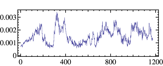
In this work, we implement the Schrödinger-functional setup on anisotropic lattices for the first time in dynamical simulations. In one of our earlier three-flavor (anisotropic) clover action simulations (with parameters $\beta=2.2$, $\rho=0.22$, $n_{\rho}=2$, $m_{0}=-0.054673$, $\gamma_{f}=\xi=3.5$), we found that the autocorrelation time of the lowest eigenvalue of $Q^{\dagger}Q$ (as defined in Eq. 4) is significantly reduced by introduction of the background field, as shown in Figure 2. Thus, for these background-field calculations, we can use correspondingly fewer trajectories compared to the calculations with antiperiodic boundary conditions.

We also implement the background field not only in the $t$ direction (as conventionally used in Schrödinger functional) but also the $z$ direction. (We label the modified masses $M_{s}$ and $M_{t}$ with respect to the direction of the boundary field direction and similarly for the mass difference $\Delta M_{s}$ and $\Delta M_{t}$.) We measure $M(x_{0})$ with various spatial $x$ and $y$ sizes, $L_{x,y}$, and sizes $L_{z}$, showing results in Figure 3, all with time extent $L_{t}=32$ and equal amount of statistics. When we increase the length in the $z$ direction, a good signal appears from $t=12$ to 16 but not beyond 24. This is because the background field becomes too weak at large $L_{z}$. When we increase the background field signal, which is proportional to $\Phi$ at $L_{z}=24$, the signal is still not as good as for $L_{z}=16$. Similar checks can be done regarding the size of $L_{x,y}$. As we increase the value from 8 to 12, the signal shows improvement. The right panel of Figure 3 zooms in the scale as seen from the left panel, and demonstrates that the $L_{x,y}=L_{z}=12$ spatial volume has the lowest statistical error while also providing enough spatial size to adequately resolve the potential which will be discussed in Section IV.2; this is the spatial volume we use in the remainder of this work.

We note that the fermion algorithm we will use corresponds to simulating the $N_{f}=3$ fermion determinant as $\det\left(Q^{\dagger}Q\right)^{\frac{3}{2}}$. In particular, when the renormalized quark mass is negative (below the chiral limit), there is no phase that should arise as in a $N_{f}=3$ version of QCD. Thus, the algorithm is implementing the absolute value of the fermion determinant. While, strictly speaking, this is not a $N_{f}=3$-flavor version of QCD when the (renormalized) quark mass is negative, it does allow us to implement a $SU(3)$ flavor symmetric version of PCAC.

II.4 Renormalization conditions

In principle, we can determine the critical values for the bare parameters $\gamma_{g}^{*}$ and all the unknown coefficients in the fermion action nonperturbatively by imposing the following conditions:

$$\xi_{g}(\gamma_{g}^{*},\gamma_{f}^{*},m_{0}^{*},c_{s}^{*},c_{t}^{*}) = \xi$$

$$\xi_{f}(\gamma_{g}^{*},\gamma_{f}^{*},m_{0}^{*},c_{s}^{*},c_{t}^{*}) = \xi$$

$$M_{t}(\gamma_{g}^{*},\gamma_{f}^{*},m_{0}^{*},c_{s}^{*},c_{t}^{*}) = m_{q}$$

$$\Delta M_{s}(\gamma_{g}^{*},\gamma_{f}^{*},m_{0}^{*},c_{s}^{*},c_{t}^{*}) = \Delta M_{s}^{(0)}$$

$$\Delta M_{t}(\gamma_{g}^{*},\gamma_{f}^{*},m_{0}^{*},c_{s}^{*},c_{t}^{*}) = \Delta M_{t}^{(0)},$$ (15)

where $\xi_{g}$ is the renormalized gauge anisotropy, $\xi_{f}$ is the renormalized fermion anisotropy (defined through the meson dispersion relation $E(p)^{2}=M^{2}+p^{2}/\xi_{f}^{2}$) and $M_{t}$ is the PCAC quark mass measured in Schrödinger functional background field (from Eq. 9). $\Delta M_{s,t}$ are the mass differences measured in two different background field directions. However, this requires that we search a five-dimensional parameter-space with dynamical simulations which is costly.

In this work, we set the spatial and temporal clover coefficients $c_{s}$ and $c_{t}$ (in Eq. ) to the tree-level tadpole-improved values. (Later in the numerical section, we demonstrate using these values that the last two conditions in Eq. 15 do hold within a few percent.) To determine the remaining three coefficients, we parameterize $\xi_{g}$, $\xi_{f}$ and $M_{t}$ as functions $f_{i}(\gamma_{g},\gamma_{f},m_{0})$. For simplicity, we choose functions of the bare parameters with the form

$$\xi_{g}(\gamma_{g},\gamma_{f},m_{0}) = a_{0}+a_{1}\gamma_{g}+a_{2}\gamma_{f}+a_{3}m_{0}$$

$$\xi_{f}(\gamma_{g},\gamma_{f},m_{0}) = b_{0}+b_{1}\gamma_{g}+b_{2}\gamma_{f}+b_{3}m_{0}$$

$$M_{t}(\gamma_{g},\gamma_{f},m_{0}) = c_{0}+c_{1}\gamma_{g}+c_{2}\gamma_{f}+c_{3}m_{0}.$$ (16)

These parameterizations are linear functions in the coefficients. We can choose higher powers of the bare parameters such as a $m_{0}^{2}$ term; however, the coefficients that we need to determine would remain linear.

Once the coefficients $a_{i}$, $b_{i}$, and $c_{i}$ are determined, we impose our renormalization conditions

$$\xi_{g}(\gamma_{g}^{*},\gamma_{f}^{*},m_{0}^{*}) = \xi$$

$$\xi_{f}(\gamma_{g}^{*},\gamma_{f}^{*},m_{0}^{*}) = \xi$$

$$M_{t}(\gamma_{g}^{*},\gamma_{f}^{*},m_{0}^{*}) = m_{q}$$ (17)

to obtain the critical values for the bare parameters as a function of the input quark mass $m_{q}$. If only linear terms in the bare parameters are used, then the intersection of these three hyperplanes is the solution of a $3\times 3$ linear system of equations. If higher-order terms are used, then the intersection is the root of a system of functions. The fitted parameters determine the chiral limit when the input $m_{q}=0$.

III Algorithm

Our configurations were generated with the Rational Hybrid Monte Carlo (RHMC) algorithm[34, 35, 36]. Strictly, RHMC refers only to the method for simulating odd flavors of fermions, and one can combine several orthogonal algorithmic improvements with the RHMC scheme resulting in a wide variety of possible RHMC algorithms. In order to be specific therefore, we describe the RHMC method in brief below and then detail our particular combination of improvements.

III.1 Rational Hybrid Monte Carlo

The basic technique for gauge generation is a Markov Chain Monte Carlo method, where one moves from an initial gauge configuration to a successive one by generating a new trial configuration and then performing an acceptance/rejection test upon it. If the trial configuration is accepted it becomes the successive configuration in the chain, otherwise if it is rejected, the original initial configuration becomes the next state in the chain.

In order to use a global Metropolis accept/reject step with a reasonable acceptance rate, the space of states is extended to include momenta $\pi_{\mu}(x)$ canonical to the gauge links $U_{\mu}(x)$ so that one may define a Hamiltonian

$$H=\frac{1}{2}\sum_{x,\mu}\pi_{\mu}(x)^{\dagger}\pi_{\mu}(x)+S(U)$$ (18)

where $S$ is the action. It is then possible to propose new configurations from previous ones by performing Molecular Dynamics (MD). Using a reversible and area preserving MD step maintains detailed balance, which is sufficient for the algorithm to converge. In order to ensure ergodicity in the entire phase space, the momenta need to change periodically. This can be affected by refreshing the momenta from a gaussian heatbath prior to the MD update step.

In order to deal with the fermion determinant, it is standard to use the method of pseudofermions. One integrates out the Grassman valued fermion fields in the action and rewrites the resulting determinant as an integral over bosonic fields as:

$$Z=\int[d\bar{\eta}][d\eta]e^{-\bar{\eta}\mathcal{D}\eta}=\det\left(\mathcal{D}\right)=\int[d\phi^{\dagger}][d\phi]e^{-\phi^{\dagger}\mathcal{D}^{-1}\phi}$$ (19)

where $\eta$ and $\bar{\eta}$ are the Grassman valued fields, $\mathcal{D}$ is some fermionic kernel and $\phi^{\dagger}$ and $\phi$ are the bosonic pseudofermion fields. Our phase space is thus enlarged to include also the pseudofermion fields, which similarly to the momenta, need to be refreshed before each MD step, to carry out the the pseudofermion integral.

In the case of a two flavor simulation, $\mathcal{D}$ is typically of the form

$$\mathcal{D}=Q^{\dagger}Q$$ (20)

where $Q$ is the fermion matrix for an individual flavor of fermion. In this case $\mathcal{D}$ is manifestly Hermitian and positive definite and the integral in Eq. 19 is guaranteed to exist. Furthermore, the pseudofermion fields can easily be refreshed by producing a vector $\chi$ filled with gaussian noise with a variance of $\frac{1}{2}$ and then forming $\phi=Q^{\dagger}\chi$.

In the case of an odd number of flavors, since $Q$ itself is not guaranteed to be positive definite, one works instead with $\sqrt{\left(Q^{\dagger}Q\right)}$ as

$$\det\left(Q\right)=\det\left(Q^{\dagger}Q\right)^{\frac{1}{2}}=\int[d\phi^{\dagger}][d\phi]e^{-\phi^{\dagger}\left(Q^{\dagger}Q\right)^{-\frac{1}{2}}\phi}\ .$$ (21)

The square root in $\mathcal{D}$ can be approximated to numerical precision using a low order rational approximation $r^{-\frac{1}{2}}(Q^{\dagger}Q)$ which can be expressed in a partial fraction (sum over poles) form as

$$\left(Q^{\dagger}Q\right)^{-\frac{1}{2}}\approx r^{-\frac{1}{2}}(Q^{\dagger}Q)=\alpha_{0}I+\sum_{k}\alpha_{k}\left[Q^{\dagger}Q+\beta_{k}\right]^{-1}\ ,$$ (22)

where the rational function approximation is specified by the coefficients $\alpha_{k}$ and $\beta_{k}$. In particular the action of all the denominator pieces onto one vector $\phi$ involves the solution of linear systems

$$\left[Q^{\dagger}Q+\beta_{k}\right]\chi=\phi$$ (23)

which can be performed simultaneously using a multiple-shift (a.k.a multi-mass) Conjugate Gradients solver[37]. Refreshment of the $\phi$ field now proceeds by evaluating:

$$\phi=r^{\frac{1}{4}}(Q^{\dagger}Q)\eta$$ (24)

where the $\eta$ are once again filled with Gaussian noise of variance $\frac{1}{2}$ and $r^{\frac{1}{4}}$ is now a rational approximation to $\left(Q^{\dagger}Q\right)^{\frac{1}{4}}$. Molecular dynamics forces now need to be calculated for each pole term in the partial fraction

$$F_{\rm rational}=-\sum_{k}\alpha_{k}\ \phi^{\dagger}\left(Q^{\dagger}Q+\beta_{k}\right)^{-1}\left[\frac{dQ^{\dagger}}{dU}Q+Q^{\dagger}\frac{dQ}{dU}\right]\left(Q^{\dagger}Q+\beta_{k}\right)^{-1}\phi.$$ (25)

The idea of using a rational approximation in the action, and its consequences for field refreshment and molecular dynamics forces make up the basics of the RHMC algorithm.

In terms of tuning, in our single precision simulations we tune the rational approximation coefficients by requiring that the approximation has a maximum error over the approximation interval that is smaller than the solver residua we require in the evaluation of the partial fraction expansions, namely $10^{-8}$ for energy calculations and $10^{-6}$ for the force calculations. Further, in the case of the force calculations we successively relax the solver criteria for poles that have smaller contributions to the force as in Refs. [34, 35, 36].

III.2 Multi-Scale Anisotropic Molecular Dynamics Update

While any reversible and area preserving MD update scheme can be used in the MD step, the acceptance rate is controlled by the truncation error in the scheme which manifests itself as a change in the Hamiltonian - $\delta H$ - over an MD trajectory since we use the Metropolis acceptance probability

$$P_{\rm acc}={\rm min}\left(1,e^{-\delta H}\right)\ .$$ (26)

We may easily construct a manifestly reversible scheme by combining symplectic update steps $\mathcal{U}_{p}(\delta\tau)$ and $\mathcal{U}_{q}(\delta\tau)$ which update momenta and coordinates by a time step of length $\delta\tau$ respectively as:

$$\mathcal{U}_{p}(\delta\tau_{\mu}):\ \left(\pi_{\mu}(x),U_{\mu}(x)\right) \rightarrow \left(\pi_{\mu}(x)+F_{\mu}(x)\delta\tau_{\mu},U_{\mu}(x)\right)$$ (27)

$$\mathcal{U}_{q}(\delta\tau_{\mu}):\ \left(\pi_{\mu}(x),U_{\mu}(x)\right) \rightarrow \left(\pi_{\mu}(x),e^{i\pi\delta\tau_{\mu}}U_{\mu}(x)\right)$$ (28)

where in the equations above $F_{\mu}(x)$ is the MD Force coming from the variation of the action with respect to the gauge fields. We emphasize, that one may update all the links pointing in direction $\mu$ with a separate step-size $\delta\tau_{\mu}$. While this may not be useful in isotropic simulations, in an anisotropic calculation with one fine direction it may be advantageous to use a shorter timestep to update the links in that direction, to ameliorate the typically larger forces that result from the shorter lattice spacing[18]. The anisotropy in step size requires a small amount of manual fine tuning, but should be similar to the anisotropy in the lattice spacings.

Our base integration scheme in this work is due to Omelyan[38, 39, 40] where we use the combined update operator

$$\mathcal{U}^{1}(\delta\tau)=\mathcal{U}_{p}(\lambda\delta\tau)\mathcal{U}_{q}(\frac{1}{2}\delta\tau)\mathcal{U}_{p}(1-{2}\lambda\delta\tau)\mathcal{U}_{q}(\frac{1}{2}\delta\tau)\mathcal{U}_{p}(\lambda\delta\tau)$$ (29)

which results in a manifestly reversible scheme that is accurate to $O(\delta\tau^{3})$. The size of the leading error term can be further minimized by tuning the parameter $\lambda$. In our work we used the value of lambda from [39] without any further tuning, which promises an efficiency increase of approximately 50% over the simple leapfrog algorithm.

In Refs. [40, 41] it was shown that a reversible, multi-level integration scheme can be constructed which allows various pieces of the Hamiltonian to be integrated at different timescales. Let us consider a Hamiltonian of the form:

$$H(\pi,U)=\frac{1}{2}\pi^{\dagger}_{\mu}(x)\pi_{\mu}(x)+S_{1}(U)+S_{2}(U)$$ (30)

where $S_{1}(U)$ and $S_{2}(U)$ are pieces of the action with corresponding MD forces $F_{1}$ and $F_{2}$ respectively. One can then split the integration into 2 timescales. One can integrate with respect to action $S_{1}(U)$ using $\mathcal{U}^{1}(\delta\tau_{1})$, where in the component $\mathcal{U}_{p}(\delta\tau_{1})$ we use only the force $F_{1}$. The whole system can then be integrated with the update:

$$\mathcal{U}^{2}(\delta\tau_{2})=\mathcal{U}^{\prime}_{p}(\lambda\delta\tau_{2})\mathcal{U}^{1}(\frac{1}{2}\delta\tau_{2})\mathcal{U}^{\prime}_{p}(1-{2}\lambda\delta\tau_{2})\mathcal{U}^{1}(\frac{1}{2}\delta\tau_{2})\mathcal{U}^{\prime}_{p}(\lambda\delta\tau_{2})$$ (31)

where in $\mathcal{U}^{\prime}_{p}$ we update the momenta using only $F_{2}$. Thus we end up with two characteristic integration timescales $\delta\tau_{1}$ and $\delta\tau_{2}$. The scheme generalizes recursively to a larger number of scales. A criterion for tuning the algorithm is to arrange for terms in the action to be mapped to different timescales so that on two timescales $i$ and $j$ we have $||F_{i}||\delta\tau_{i}\approx||F_{j}||\delta\tau_{j}$, as suggested in Ref. [42]. We now proceed to outline how we split our action.

III.3 Even Odd Preconditioning the Clover Term

The clover term may be preconditioned by labeling sites as even and odd, and grouping together the terms in the operator that connect sites of various labels. In particular

$$Q=\left(\begin{array}[]{cc}A_{ee}&D_{eo}\\ D_{oe}&A_{oo}\end{array}\right),$$ (32)

where the blocks $A_{ee}$ and $A_{oo}$ contain the clover term and the diagonal parts of the Wilson operator whereas the $D_{eo}$ and $D_{oe}$ contain the Wilson hopping term. This matrix can be block diagonalized as

$$Q=\left(\begin{array}[]{cc}1&0\\ D_{oe}A^{-1}_{ee}&1\end{array}\right)\left(\begin{array}[]{cc}A_{ee}&0\\ 0&A_{oo}-D_{oe}A^{-1}_{ee}D_{eo}\\ \end{array}\right)\left(\begin{array}[]{cc}1&A^{-1}_{ee}D_{eo}\\ 0&1\\ \end{array}\right)$$ (33)

and it is clear that

$$\det\left(Q\right)=\det\left(A_{ee}\right)\det\left(A_{oo}-D_{oe}A^{-1}_{ee}D_{eo}\right)$$ (34)

and we can write an action containing $N_{f}$ degenerate fermion flavors as:

$$\det\left(Q^{\dagger}Q\right)^{\frac{N_{f}}{2}}=e^{\sum_{x}N_{f}\mbox{tr}\,\log A_{ee}(x)-\sum_{i=1}^{N_{f}}\phi^{\dagger}_{i}\left[r^{-\frac{1}{2}}(\tilde{Q}^{\dagger}\tilde{Q})\right]\phi_{i}}$$ (35)

with the preconditioned fermion matrix

$$\tilde{Q}=A_{oo}-D_{oe}A^{-1}_{ee}D_{eo}$$ (36)

This manner of preconditioning the clover term is quite standard, in particular guides to implementation are detailed in Ref. [42]. We mention that it may be possible to combine the three pseudofermion terms each containing $r^{-\frac{1}{2}}(\tilde{Q}^{\dagger}\tilde{Q})$ into a single one containing instead a single rational approximation $r^{-\frac{3}{2}}$, however the Remez algorithm for this approximations results in negative roots with dire implications for our multi-shift solver. In this work therefore, we have simulated with three separate one flavor pseudofermion terms.

It was our experience that the forces resulting from the $\mbox{tr}\,\log A_{ee}$ terms were at least an order of magnitude smaller than the pseudofermion terms, and so the two kind of terms could be run on separate timescales.

III.4 Stout Link Smearing in Fermion Actions

The fermionic terms in our action employ stout link smearing[20] on the links in the spatial direction. We leave the temporal direction unsmeared to keep the transfer matrix physical. The Schrödinger functional boundary condition is imposed at every iteration of the stout-link smearing. Our fermion operator $\tilde{Q}$ is evaluated on the stout smeared fields. In the calculation of the fermion forces we compute the force on the stouted links, but then have to also apply the chain rule to compute the force coming from the original thin links viz:

$$\frac{d\tilde{Q}}{dU_{\rm thin}}=\frac{d\tilde{Q}}{dU_{\rm stout}}\frac{dU_{\rm stout}}{dU_{\rm thin}}$$ (37)

In particular the $\frac{dU_{\rm stout}}{dU_{\rm thin}}$ term is common to all the poles in the rational function approximation, hence in our rational forces computations we compute all the forces with respect to the stout links first and then perform the recursion to the thin links only once. The Schrödinger functional boundary conditions imply that the force for the links which we hold fixed are set to zero.

III.5 Split Gauge Term

We can write our gauge action schematically as

$$S=S_{s}(U)+S_{t}(U),$$ (38)

where the term $S_{s}$ contains only loops with spatial gauge links, and the $S_{t}$ term contains loops contain spatial and temporal links. While the term $S_{s}$ produces forces only in the spatial directions, the $S_{t}$ term produces forces in both the spatial and the temporal directions. In particular the spatial forces from $S_{t}$ are larger in magnitude than the spatial forces from $S_{s}$ by roughly the order of the anisotropy, and in turn, the temporal forces from $S_{t}$ are larger than the spatial forces from $S_{t}$. Our anisotropic integration step-size balances the spatial and temporal forces of the $S_{t}$ term against each other, however in order to balance the spatial forces from $S_{t}$ and $S_{s}$ against each other we integrate them on separate time scales.

III.6 Summary

To summarize, we use the RHMC algorithm, with approximations tuned separately for the force and energy calculations. Our molecular dynamics scheme uses anisotropic timesteps and a recursively defined multi-level integration scheme based on Omelyan’s inverter. Our fermionic terms employ stout smearing in the spatial directions only. We have 4 kinds of terms in our molecular dynamics integration, namely the $\mbox{tr}\,\log A_{ee}$ term, the $\phi^{\dagger}_{i}r^{-\frac{1}{2}}(\tilde{Q})\phi$ pseudofermionic terms, the spatial gauge action term $S_{s}$ and the temporal gauge action term $S_{t}$.

Based upon the magnitude of the molecular dynamics forces, we split our integration scheme onto three time scales

• Time scale 1 uses the Omelyan integrator with a timestep of $\delta t_{1}$, and contains the $\mbox{tr}\,\log A_{ee}$ term and the pseudofermion terms.

• Time scale 2 uses a leapfrog integrator with a timestep of $\delta t_{2}$ relative to time scale 1, and contains the spatial gauge action term.

• Time scale 3 uses a leapfrog integrator with a timestep of $\delta t_{3}$ relative to time scale 2, and contains the temporal gauge action term.

For our $12^{3}\times 32$ volume results with a background field, we used timesteps $(\delta t_{1},\delta t_{2},\delta t_{3})=(1/4,1/4,1/3)$ for the three time scales, and for our $12^{3}\times 96$ volume results with antiperiodic boundary conditions we used $(1/5,1/3,1/2)$. In addition, the time step for the temporal direction was a factor of $\xi=3.5$ times smaller than the spatial timesteps. The acceptance rate was typically between 60 and 70%. These technologies are all implemented in the Chroma Software System [25] .

IV Numerical Results

We are interested in a spatial lattice spacing on the order of 0.1–0.2 fm with a target anisotropy of $\xi=3.5$, which would provide a fine-enough temporal lattice spacing for excited-state physics. We proceeded by making an initial guess for the anisotropy parameters, $\gamma_{g}=\gamma_{f}=\xi=3.5$ and $m_{0}=-0.05$, and computed the Sommer scale $r_{0}/a_{s}$ (Ref. [43]) over a range of $\beta$ with lattice sizes of $12^{3}\times 32$. Anticipating significant running in $r_{0}/a_{s}$, we chose to use $\beta=1.5$. A preliminary investigation indicates a lattice spacing of roughly $0.12$ fm. However, a careful determination of the lattice spacing involves a study of the static quark potential as well as hadron masses on $N_{f}=2+1$ ensembles, a determination of the strange quark mass, extrapolation of the light quark mass to the physical limit, and examining different approaches to include potential systematic uncertainties which will be presented in Ref.[44]. Note that in the earlier part of this section, we will vary $\beta$ to make a global search and to get an understanding of the stout-smearing parameters and tadpole factors.

We tune the gauge and fermion anisotropies in three-flavor simulations. The determination of the tadpole factors used in the gauge and fermion action and the stout-link parameter study will be described in Subsec. IV.1. We ultimately decide to 3d stout-link smear with $n_{\rho}=2$ and $\rho=0.14$. Subsec. IV.2 and IV.3 describe how the gauge and fermion anisotropies are measured, and finally the target coefficients in the fermion action are determined in Subsec. IV.4.

IV.1 Plaquette, Tadpole Factors and Stout Links

In this work, we tadpole improve [45] the gauge and fermion actions. This procedure amounts to replacing the gauge link fields with $\hat{U}_{\mu}(x)=U_{\mu}(x)/u$. We obtain the tadpole factors used in the simulation from a nonperturbative tuning. There are two types of tadpole factors; we denote using $\tilde{u}_{s,t}$ the tadpole factors with the stout-smeared fields (which are used in the gauge links of the fermion action), and ${u}_{s,t}$ are those without smearing (which are in the gauge action). For each parameter set, we start with a perturbative guess, $u_{s}=u_{t}=1$, and calculate the actual $u_{s,t}$ from the plaquette. Then, we use the new value to feed back into the next dynamical run. The value of $u_{s,t}$ will converge, giving the nonperturbative value with 1–2% precision.

We calculated these tadpole factors with a large range of $\beta$ values in three-flavor simulations. Over a wide range of parameters, we find that the square root of the spatial plaquette is consistent with the temporal plaquette, for both smeared and unsmeared links, indicating that the temporal tadpole factor is close to one. We chose to fix $u_{t}=\tilde{u}_{t}=1$ throughout the remainder of the work. It still remains to determine the spatial tadpole factors.

Let us first concentrate on the influence of the stout-smearing parameters on the plaquette. In Sec. II, we set the stout-link parameters to be $\rho=0.22$ and $n_{\rho}=2$, following the choice of the two-flavor anisotropic study done in Ref. [18]. At one-loop level we expect the spatial plaquette to be

$$\langle{\cal P}_{s}\rangle = 1-c_{ss}^{(1)}g^{2}$$ (39)

where $c_{ss}^{(1)}$ is a function of the gauge action and stout-link parameters. Figure 4 shows $c_{ss}^{(1)}$ as a function of $\rho$ for $n_{\rho}=1,2,3$, as calculated in Ref. [46] with our choice of a Symanzik-improved gauge action. We find that the choice of $\rho=0.14$ corresponds to a minimum of $c_{ss}^{(1)}$ which corresponds to the maximum of the spatial plaquette in Eq. 39 for $g^{2}>0$. We note that this value of $\rho=0.14$ is also consistent with the suggestion [47] that the maximum allowable value, given by a classical argument, is $1/6$ in our case of three-dimensional smearing. We also investigate the spatial plaquettes in our numerical studies; see Figure 5. In this investigation, we use three different three-flavor ensembles with sea-sector parameters as follow:

• Ensemble A: $\beta=2.0$, $\gamma_{g}=3.5$, $\gamma_{f}=3.89$, $\{\rho,n_{\rho}\}=\{0.22,2\}$

• Ensemble B: $\beta=2.0$, $\gamma_{g}=3.5$, $\gamma_{f}=3.5$, $\{\rho,n_{\rho}\}=\{0.14,1\}$

• Ensemble C: $\beta=1.0$, $\gamma_{g}=3.0$, $\gamma_{f}=3.33$, $\{\rho,n_{\rho}\}=\{0.22,2\}$

with fixed $m_{0}=0$, $12^{3}\times 32$ volume with antiperiodic boundary conditions in time. We vary $\rho$ in the valence sector and study the resulting behavior of the spatial plaquettes. We find that plaquette is maximized in the vicinity close to our initial choice $\rho=0.22$.

We then concentrate on one set of fermion coefficients, $\rho=0.14$, $m_{0}=0$, $\gamma_{g}=3.5$, and $\gamma_{f}=3.5$, and study the tadpole factors as functions of $\beta$ with two values of $n_{\rho}$, as shown in Figure 6. We see that the fermion stout-link smeared tadpole factor $\tilde{u}_{s}$ (denoted as $u_{s}^{\rm(st)}$ in the plot) increases when we double the number of smearing steps and gets closer to one, which is what we expected. The gauge tadpole factor (without stout-link smearing, denoted as $u_{s}^{(\rm un)}$) remains unchanged, as if the stout-smearing in fermion sector had no impact in the gauge sector. This tells us the ultraviolet observable does not change with $n_{\rho}=2$; therefore, in the rest of this paper, we will fix the smearing parameters to $\rho=0.14$ and $n_{\rho}=2$.

We parameterize the smeared and unsmeared spatial tadpole factors as

$$u = \sum_{n=1}^{3}\frac{1+a_{n}g^{2n}}{1+b_{n}g^{2n}}$$ (40)

with the constraint $a_{1}-b_{1}=c^{(1)}$, where $g^{2}$ is defined as $6/\beta$ and $c^{(1)}$ is the one-loop perturbative value of the tadpole factor [46]. Figure 7 shows the data for $n_{\rho}=2$ and $\rho=0.14$ and the fit using Eq. 40. The tadpole factors are interpolated well over a large range of $\beta$. At $\beta=1.5$ (on which we will focus for the rest of the paper) this parameterization gives:

$$u_{s}=0.7336,\ \qquad\tilde{u}_{s}=0.9267.$$ (41)

In all further investigations, we use the values as determined by Eq. 40. We note that as we vary $\beta$, anisotropies and masses, the values predicted by Eq. 40 agree to a few percent.

Figure 4: The one-loop coefficient of the spatial plaquette, $c_{ss}^{(1)}$, as a function of $\rho$ for $n_{\rho}=1,2,3$. The minimum $c_{ss}^{(1)}$ (where the plaquette is near 1) in all three cases, as shown above, indicates $\rho\approx 0.14$.

Figure 5: This graph shows how the spatial stout-smeared plaquette varies as a function of valence stout parameter, $\rho$, on three different ensembles with different choices of fermion parameters, $\beta$ and stout-smearing factors, as indicated in the legend box. The smeared threshold is only observed for $\rho_{\rm thresh}\leq 0.2$ in $\beta=2.0$ case; for smaller $\beta$, the maximum $\rho_{\rm thresh}\approx 0.25$.

Figure 6: The self-consistent tadpole factors as a functions of $\beta$ at fixed $m_{0}$, $\gamma_{g}=\gamma_{f}=\xi=3.5$ and $u_{t}=\tilde{u}_{t}=1$. The unsmeared spatial tadpole factors $u_{s}^{\rm(un)}$ are nearly identical for both $n_{\rho}=1$ and $n_{\rho}=2$.

Figure 7: Padé approximation for tadpole factors $u_{s}$ and $u_{s}^{\rm(st)}$ for $n_{\rho}=2$.

IV.2 Gauge Anisotropy

We determine the gauge anisotropy from the static-quark potential using Klassen’s “Wilson-loop ratio” approach [48]. In this method, we use Wilson loops involving the temporal direction, $W_{st}$, and those in the spatial directions, $W_{ss}$, with Schrödinger functional boundary conditions applied in the $z$ direction. We measure the ratios

$$R_{ss}(x,y) = \frac{W_{ss}(x,y)}{W_{ss}(x+1,y)}\xrightarrow{\rm asym}e^{-a_{s}V_{s}(ya_{s})},$$

$$R_{st}(x,t) = \frac{W_{st}(x,t)}{W_{st}(x+1,t)}\xrightarrow{\rm asym}e^{-a_{s}V_{s}(ta_{t})}$$

on lattice volumes of $12^{3}\times 32$. Naturally, one should impose $R_{ss}(x,y)=R_{st}(x,t)$ to get the renormalized $\xi_{g}$. An advantage to this method is that finite-volume artifacts tend to cancel in the ratios as demonstrated in the case of the (quenched) Wilson gauge action [48] and the Iwasaki gauge action [17] with dynamical fermions. We determine $\xi_{g}$ by minimizing [17]

$$L(\xi_{g})=\sum_{x,y}\frac{(R_{ss}(x,y)-R_{st}(x,\xi_{g}y))^{2}}{(\Delta R_{s})^{2}+(\Delta R_{t})^{2}},$$ (43)

where $\Delta R_{s}$ and $\Delta R_{t}$ are the statistical errors of $R_{ss}$ and $R_{st}$. We interpolate $R_{st}(x,t)$ by a cubic spline in terms of $t$. To avoid short-range lattice artifacts, $x$ and $y$ should not be too small. It has been observed in the $N_{f}=2$ case [17] that including data with $y=1$ introduces significant artifacts due to excited-state contamination.

While this method was originally proposed for use in gauge actions with periodic boundary conditions, we note that it can also be applied to the case of a constant background field. The basic observation is that if we use Wilson loops orthogonal to the background field direction (the boundary condition direction), the flux from the background field that propagates should cancel in the ratios $R_{ss}$ or $R_{st}$. To confirm this, we measured $\xi_{g}$ with two different three-flavor ensembles with the same action parameters $\beta=1.5$, $\gamma_{g}=4.4$, $m_{0}=-0.0570$ and $\gamma_{f}=3.3$ but under two boundary conditions: Schrödinger functional and periodic boundary conditions in the $z$ direction. Figure 8 shows the results from both measurements. The gauge anisotropy from periodic boundaries, $\xi_{g}^{\rm PBC}$, as a function of $\min(xy)$ is plotted. Compared with two-flavor simulation [17], the three-flavor results show larger dependence on $\min(xy)$. The band in Figure 8 is the resulting gauge anisotropy from Schrödinger functional boundaries, $\xi_{g}^{\rm SF}$, (obtained from $\min(xy)=4$); it is consistent with $\xi_{g}^{\rm PBC}$. We gain advantages by calculating $\xi_{g}^{\rm SF}$ instead of $\xi_{g}^{\rm PBC}$ for reasons described in Subsec. II.3. Therefore, for the rest of this work, we will use the gauge anisotropy $\xi_{g}^{\rm SF}$ as $\xi_{g}$.

Figure 8: Consistency check on $\xi_{g}$ measured in Schrödinger functional boundary conditions (band) and periodic boundary conditions (points) as functions of the product of $x$ and $y$. The fermion action parameters for this run are $\gamma_{g}=4.4$, $m_{0}=-0.0570$ and $\gamma_{f}=3.3$.

IV.3 Fermion Anisotropy

We determine the fermion anisotropy $\xi_{f}$ through the conventional relativistic meson dispersion relation

$$E(\vec{p})^{2}=m^{2}+\frac{\vec{p}^{2}}{\xi_{f}^{2}}$$ (44)

where the energy $E$ and the mass $m$ are in units of $a_{t}$, and $\vec{p}=2\pi\vec{n}/L_{s}$, with $L_{s}$ the spatial lattice size, is in units of $a_{s}$. Gauge configurations are generated using periodic boundary conditions in space and antiperiodic in time on lattice volumes of $12^{3}\times 96$. We use six equally separated time sources, two different source quark smearings and an unsmeared (local) sink to produce the correlators. These are then averaged over the six time sources. The two resulting hadron correlators for each momentum, averaged over equivalent rotations, were used in a constrained fit to two amplitudes and one mass. These results are also cross-checked against a fit including two masses (a ground and excited state).

We calculate the energy $E(\vec{p})$ at the spatial momenta $\vec{p}=2\pi\vec{n}/L_{s}$ for $n=(0,0,0)$, $(1,0,0)$, $(1,1,0)$, and $(2,0,0)$. The resulting jackknife energies are used in a linear fit (in $E(\vec{p})^{2}$) to Eq. 44 to extract $\xi_{f}$. We find no significant deviation from linearity. An example is in Figure 9 which shows the pseudoscalar and vector meson energies with action parameters $\beta=1.5$, $\gamma_{g}=4.4$, $m_{0}=-0.0540$ and $\gamma_{f}=3.3$ at multiple momentum projections. (The effective energy is shown as $\ln(C(t+1)/C(t))$.) We measure $\xi_{f}=3.44(8)$ from the pseudoscalar meson and $\xi_{f}=3.44(10)$ from the vector meson, which are consistent.

In our earlier work, we determined the fermion anisotropy through the PCAC mass ratio from Schrödinger functional boundary conditions in the $z$ and $t$ directions. However, unlike the case of the Wilson loop, we found it difficult to exclude excited-state contamination with the limited size of the spacial direction; thus, such a method suffers from a larger systematic error due to the extraction of the PCAC mass. We also investigated using the Schrödinger-functional scheme with Dirichlet (zero) gauge boundary conditions and a point-like (but smeared) fermion boundary condition [49] in time allowing us to project our correlators onto non-zero momenta, and thus allowing an extraction of the fermion anisotropy from the meson dispersion relation. This method, however, did not give as reliable results as in the antiperiodic case. Therefore, we choose to use the meson dispersion to determine $\xi_{f}$ on (anti)periodic boundary gauge ensembles.

Figure 9: Effective mass plots for various momentum projections of the pseudoscalar (left) and vector (right) mesons and corresponding fits. The fermion action parameters for this run are $m_{0}=-0.0540$, $L_{t}=96$, $\gamma_{g}=4.4$ and $\gamma_{f}=3.3$ with (anti)periodic boundary conditions.

IV.4 Tuning Result

With $\beta$ fixed at $1.5$, we only need to tune the parameters $\gamma_{g}$, $\gamma_{f}$ and $m_{0}$. Our strategy is to choose some suitable estimates of the anisotropies, and make a coarse scan in $m_{0}$ to find the region of the critical point as determined from the PCAC mass $M_{t}$, where, as described in Sec. II.3 a background field in the $t$ direction was used. Due to the nice properties of the algorithm in the background field, fairly short runs over roughly 1000 trajectories with measurements every fifth trajectory are sufficient for the purpose of determining $M_{t}$. Given a mass regime of interest, the gauge anisotropy $\xi_{g}$ is determined using a background in the $z$ direction as described in Sec. IV.2. Again, roughly 1000 trajectories are sufficient. The measurements of $M_{t}$ and $\xi_{g}$ used $12^{3}\times 32$ volumes, and provide a reasonable range of the bare parameters $m_{0}$ and $\gamma_{g}$ for further determinations of the fermion anisotropy $\xi_{f}$. These latter measurements used the method described in Sec. IV.3 on $12^{3}\times 96$ volumes with antiperiodic boundary conditions in time. Longer runs of roughly 2000 trajectories are used with measurements every fifth trajectory and binned twice, so they are effectively measured every tenth trajectory.

Of course, each of these simulations are independent of one another. The ensemble parameters, and the results of the determinations of $M_{t}$, $\xi_{g}$, and $\xi_{f}$ are summarized in Table 1, Table 2, and Table 3, respectively.

For each measurement, we fit the data according to the linear ansatz in Eq. 16. The fit parameters are

$$a_{0} =0.5(8), \quad a_{1} =0.41(14), \quad a_{2} =0.39(8), \quad a_{3} =1.3(7)$$

$$b_{0} =-4.8(12), \quad b_{1} =0.6(2), \quad b_{2} =1.74(17), \quad b_{3} =4(3)$$

$$c_{0} =0.395(18), \quad c_{1} =-0.082(3), \quad c_{2} =0.0194(17), \quad c_{3} =1.282(16)\quad.$$ (45)

The values of $\chi^{2}$ per degree of freedom are $6.0/16$, $13.2/8$, $34.7/17$ respectively. Figures 10, 11 and 12 demonstrate how the fits work using two-dimensional slices of the parameter and measurement spaces. Both $\xi_{g}$ and $\xi_{f}$ show little sensitivity to the parameter $m_{0}$, and thus the slope is poorly determined in our fits. However, we do not expect this would affect our final result much since the change in $m_{0}$ are of the magnitude of $O(10^{-2})$ and the $\xi_{g}$ and $\xi_{f}$ are of the size of $O(1)$. The interactions of $\xi_{g}$ and $\xi_{f}$ also have large uncertainties in the fits; this is also expected since the running coefficients, $\gamma_{f}$ and $\gamma_{g}$, are around 3–4 and there is a long extrapolation to 0. In terms of fits to $M_{t}$, $m_{0}$ has the dominant effect, a few times larger than the $\gamma_{g}$ while $\gamma_{f}$ has one magnitude smaller contribution. We found that $\xi_{g}$ and $\xi_{f}$ have positive linear dependence on the bare parameters, while for the case of $M_{t}$ versus $\gamma_{g}$, we found that $M_{t}$ increases while $\gamma_{g}$ decreases. The $\gamma_{g}$ parameter is the dominant factor in $\xi=a_{s}/a_{t}$. Increasing it, $a_{t}$ will increase as well; this leads to the only non-dimensionless measurement $M_{t}$ becoming smaller in units of $a_{t}$. Similar effects are observed when we parameterize the pion mass squared or rho-meson mass (which are measured on the antiperiodic boundary condition ensemble); see Figure 13 and 14.

We can gain a qualitative understanding of the origin of the opposite sign in the slopes of $\gamma_{g}$ versus $\gamma_{f}$ for the mass measurements by considering the classical dispersion relation for the action in Eq. . For a small background chroma-electric field $F_{0i}$, we find that the lattice dispersion relation energy at zero spatial momentum $\hat{E}=2\sinh(a_{t}m_{0})/a_{t}$ satisfies for our choice of clover coefficient $c_{t}$ from Eq. 5

$$\hat{E}^{2}(1+a_{t}m_{0})=m_{0}^{2}-\left(\frac{\gamma_{g}}{\gamma_{f}}+\frac{1}{2}\left(\xi\frac{\gamma_{g}}{\gamma_{f}}+1\right)\sinh(a_{t}m_{0})\right)\sum_{i}\sigma_{0i}F_{0i}\quad.$$ (46)

Thus, the derivatives $\partial\hat{E}^{2}/{\partial\gamma_{g}}\propto-F_{0i}$ and $\partial\hat{E}^{2}/{\partial\gamma_{f}}\propto+F_{0i}$ have opposite sign.

We impose the renormalization condition that in the chiral limit $\{\xi_{g},\xi_{f},M_{t}\}=\{3.5,3.5,0\}$. By solving Eq. 17 with the parameters in Eq. 45, we found that

$$\{m_{cr},\gamma_{g}^{*},\gamma_{f}^{*}\}=\{-0.080(6),4.38(8),3.44(7)\}.$$ (47)

By fixing the renormalization condition in the general case, $\{\xi_{g},\xi_{f},M_{t}\}=\{3.5,3.5,m_{q}\}$, we obtain the desired action parameters as a functions of the bare quark mass, as shown in Fig. 16. As emphasized in the discussions above, $\gamma_{g}^{*}$ and $\gamma_{f}^{*}$ have very small quark mass dependence from the chiral limit up to the heaviest $m_{0}$ used in this work, $-0.057$ (which corresponds to $m_{q}\approx 0.03$). Of course, $m_{0}$ is linearly proportional to the bare quark mass.

Figure 15 shows a subset of the $m_{0}$ values with their corresponding gauge and fermion anisotropies. The two simulation points that are consistent with the desired points of $\{\xi_{g},\xi_{f}\}=\{3.5,3.5\}$ are consistent with Eq. 47.

Based upon the negligible mass dependence that is observed, we henceforth fix the anisotropy bare parameters to

$$\gamma_{g}^{*}=4.3,\quad\gamma_{f}^{*}=3.4$$ (48)

which corresponds to a parameter set used in Figure 15. The corresponding clover coefficients are

$$c_{s}=1.589,\quad c_{t}=0.903.$$

Figure 17 shows a PCAC measurement as a function of $m_{0}$ with $\beta=1.5$, $\gamma_{g}=4.4$, and $\gamma_{f}=3.3$; and linear interpolation to $M_{t}=0$ gives us

$$a_{t}m_{cr}=-0.0854(5)\quad.$$ (49)

Finally, we will discuss how our initial tadpole-improved clover coefficients $c_{\rm s,t}$ differ from the nonperturbative coefficients in the Schrödinger functional scheme (as described in Sec. II.3). Table 1 lists the PCAC mass, $\Delta M_{t}$ and its tree-level value (in units of $a_{t}^{-1}$) measured with the $t$-direction Schrödinger functional boundary condition. If we had nonperturbatively tuned $c_{s,t}$ and imposed the renormalization conditions from Eq. 15, we should expect that $\Delta M_{t}=\Delta M_{t}^{(0)}$. There are four sets of ensemble parameters that satisfy the conditions on $\gamma_{g}^{*}$ and $\gamma_{f}^{*}$. If we extrapolate $\Delta M_{t}$ to $m_{cr}$, we find $\Delta M_{t}=-0.00022(57)$, which is about 1.5 standard deviations away from the tree-level value: $-0.00167$. (See Figure 18.) We conclude that the tadpole-corrected tree-level coefficients with stout-link smearing are close enough to the nonperturbative $O(a)$-improved coefficients in the three-flavor dynamical simulation.

Figure 10: Gauge anisotropy as a function of $\gamma_{g}$, $\gamma_{f}$ at fixed $m_{0}$. The straight lines are the fit functions in Eq. 16 keeping the remaining two parameters fixed. Table 2 lists the details of the ensemble parameters.

Figure 11: Fermion anisotropy as a function of $\gamma_{g}$, $\gamma_{f}$ at fixed $m_{0}$. Table 3 lists the details of the ensemble parameters.

Figure 12: PCAC mass (in units of the temporal lattice spacing) as a function of $\gamma_{g}$, $\gamma_{f}$ at fixed $m_{0}$. Table 1 lists the details of the ensemble parameters.

Figure 13: Pion mass squared (in units of $a_{t}^{-2}$) as a function of $\gamma_{g}$, $\gamma_{f}$ at fixed $m_{0}$. Table 3 lists the details of the ensemble parameters.

Figure 14: Rho-meson mass (in units of $a_{t}^{-1}$) as a function of $\gamma_{g}$, $\gamma_{f}$ at fixed $m_{0}$. Table 3 lists the details of the ensemble parameters.

Figure 15: Renormalized gauge and fermion anisotropies (left) and the corresponding bare parameter (left). The detailed parameters can be found in Table 3 and Table 2. Note that the predicted coefficients from fitting Eq. 17 in the chiral limit are $\{\gamma_{g}^{*},\gamma_{f}^{*}\}=\{4.38(8),3.44(7)\}$.

Figure 16: Tuned gauge and fermion action parameters, $m_{0}$ (top), $\gamma_{g}^{*}$ (middle) and $\gamma_{f}^{*}$ (bottom), as functions of the bare quark mass, $a_{t}m_{q}$, corresponding to the solution of Eq. 17. There is negligible mass dependence in the tuned anisotropy parameters. With a spatial lattice spacing $a_{s}=0.12$ fm, the maximum extend of the horizontal axis is about $175$ MeV.

Figure 17: PCAC mass at $\beta=1.5$, $\gamma_{g}=4.3$ and $\gamma_{f}=3.4$ as a function of $m_{0}$. A linear interpolation gives $m_{\rm cr}=-0.0854(5)$.

Figure 18: The measured $\Delta M_{t}$ (down triangles) in units of $a_{t}$ as a function of $m_{0}$ at fixed $\gamma_{g}=4.3$ and $\gamma_{f}=3.4$, along with $\Delta M_{t}^{(0)}$ (dashed line)

Table 1: PCAC mass (in units of the inverse temporal lattice spacing) measured from the $t$-direction Schrödinger functional boundary condition ensemble with volume $12^{3}\times 32$.

$m_{0}$	$\gamma_{g}$	$\gamma_{f}$	$M_{t}$	$\Delta M_{t}$	$\Delta M_{t}^{(0)}$
$-$0.0950	4.3	3.5	$-$0.0122(9)	0.0003(10)	$-$0.001547
$-$0.0950	4.3	3.4	$-$0.0121(9)	0.0003(9)	$-$0.00167
$-$0.0950	4.3	3.3	$-$0.0141(8)	0.0002(9)	$-$0.001798
$-$0.0734	4.3	3.5	0.0160(9)	$-$0.0007(9)	$-$0.001547
$-$0.0734	4.3	3.4	0.0149(7)	$-$0.0007(6)	$-$0.00167
$-$0.0734	4.3	3.3	0.0139(7)	0.0006(11)	$-$0.001798
$-$0.0618	4.2	3.5	0.0431(11)	0.0002(4)	$-$0.001427
$-$0.0618	4.2	3.4	0.036(2)	$-$0.0004(8)	$-$0.001545
$-$0.0618	4.2	3.3	0.0339(11)	0.0004(8)	$-$0.001672
$-$0.0618	4.3	3.5	0.0321(9)	0.0003(5)	$-$0.001547
$-$0.0618	4.3	3.4	0.0303(6)	$-$0.0001(5)	$-$0.00167
$-$0.0618	4.3	3.3	0.0297(6)	$-$0.0003(4)	$-$0.001798
$-$0.0618	4.4	3.4	0.0218(5)	$-$0.0004(5)	$-$0.001791
$-$0.0618	4.4	3.3	0.0213(7)	0.0001(6)	$-$0.001923
$-$0.0570	4.3	3.4	0.0349(7)	0.0002(5)	$-$0.00167
$-$0.0570	4.3	3.3	0.0342(10)	0.0004(7)	$-$0.001798
$-$0.0570	4.3	3.2	0.0311(12)	0.0005(8)	$-$0.001935
$-$0.0570	4.3	3.1	0.0300(9)	0.0025(8)	$-$0.002078
$-$0.0570	4.4	3.3	0.0248(12)	0.0002(8)	$-$0.001923
$-$0.0570	4.4	3.2	0.0239(6)	0.0005(7)	$-$0.002065
$-$0.0570	4.4	3.1	0.0220(7)	0.0012(11)	$-$0.002212

Table 2: Renormalized gauge anisotropy measured from the $z$-direction Schrödinger functional boundary condition ensemble with volume $12^{3}\times 32$.

$m_{0}$	$\gamma_{g}$	$\gamma_{f}$	$\xi_{g}$
$-$0.0950	4.3	3.5	3.48(5)
$-$0.0950	4.3	3.4	3.42(3)
$-$0.0950	4.3	3.3	3.40(3)
$-$0.0743	4.3	3.4	3.47(10)
$-$0.0734	4.3	3.4	3.46(4)
$-$0.0618	4.2	3.5	3.48(4)
$-$0.0618	4.2	3.4	3.41(3)
$-$0.0618	4.2	3.3	3.42(2)
$-$0.0618	4.3	3.5	3.50(4)
$-$0.0618	4.3	3.4	3.47(4)
$-$0.0618	4.3	3.3	3.43(4)
$-$0.0618	4.3	3.2	3.38(7)
$-$0.0618	4.4	3.3	3.47(5)
$-$0.0570	4.3	3.4	3.48(7)
$-$0.0570	4.3	3.3	3.43(9)
$-$0.0570	4.3	3.2	3.39(3)
$-$0.0570	4.3	3.1	3.36(4)
$-$0.0570	4.4	3.3	3.50(4)
$-$0.0570	4.4	3.2	3.54(5)
$-$0.0570	4.4	3.1	3.399(16)

Table 3: Fermion anisotropy, vector-meson mass and pseudoscalar mass squared (in units of the inverse temporal lattice spacing) from the periodic boundary condition ensemble with volume $12^{3}\times 96$.

$m_{0}$	$\gamma_{g}$	$\gamma_{f}$	$\xi_{f}$	$m_{\pi}$	$m_{\rho}$	$m_{\pi}/m_{\rho}$
$-$0.0743	4.3	3.4	3.43(4)	0.1501(9)	0.222(3)	0.677(9)
$-$0.0618	4.2	3.5	3.62(5)	0.2830(9)	0.348(2)	0.814(5)
$-$0.0618	4.2	3.4	3.38(4)	0.2753(10)	0.337(2)	0.816(5)
$-$0.0618	4.2	3.3	3.18(3)	0.2604(10)	0.319(5)	0.817(11)
$-$0.0618	4.3	3.4	3.47(6)	0.2232(15)	0.290(4)	0.769(9)
$-$0.0618	4.4	3.3	3.25(6)	0.1639(17)	0.217(5)	0.754(16)
$-$0.0570	4.3	3.3	3.23(4)	0.2401(13)	0.299(4)	0.804(8)
$-$0.0570	4.3	3.2	3.19(5)	0.2290(16)	0.292(4)	0.784(10)
$-$0.0570	4.3	3.1	2.99(4)	0.2164(18)	0.261(7)	0.828(20)
$-$0.0570	4.4	3.3	3.43(6)	0.193(3)	0.255(6)	0.758(17)
$-$0.0570	4.4	3.2	3.22(8)	0.182(3)	0.233(5)	0.780(17)
$-$0.0570	4.4	3.1	2.91(11)	0.151(3)	0.194(6)	0.78(2)

V Conclusion and Outlook

This is the first calculation that combines Schrödinger functional with stout-link smearing on three-flavor anisotropic clover action. The Schrödinger functional boundary conditions allow us to work on small volumes and small quark masses with improved signal, which improves our ability to probe the chiral limit. Stout-link smearing improves the chiral and scaling properties of our chirally broken fermion action. We take advantage of the much smaller cost by implementing both in our calculation.

We studied a range of stout-link parameters that may be safely applied to multiple choices of $\beta$ and different coefficients in the fermion sector in three-flavor simulation. Although our numerical simulations suggested that higher values of $\rho$ could be applied, in the end, the stout-link parameters we chose conservatively to be $\rho=0.14$ and $n_{\rho}=2$, as suggested by a one-loop perturbative calculation.

In a preliminary three-flavor study of various $\beta$ values, we found through the static quark potential that $\beta=1.5$ gave us the desired spatial lattice spacing around $0.12$ fm in the physical limit. The remaining coefficients in the gauge action and clover coefficients $c_{s,t}$ in the fermion action were set to their tree-level tadpole improved values, which were numerically determined and interpolated using a Padé approximation.

We determined the gauge anisotropy using Wilson-loop ratios and Schrödinger functional boundary conditions in the $z$ direction; we determined the fermion anisotropy using antiperiodic boundary conditions in time. The quark mass was estimated from PCAC measurements using Schrödinger functional boundary conditions in the $t$ direction from which we found the critical mass.

We then tuned the remaining parameters $\xi_{g,f}$ to achieve the desired renormalized anisotropy $\xi=3.5$ in the chiral limit. We found $\{m_{cr},\gamma_{g}^{*},\gamma_{f}^{*}\}=\{-0.080(6),4.38(8),3.44(7)\}$ from a linear parameterization. The mass dependence of the gauge and fermion anisotropies is found to be negligible. Hence, we have for the final parameters

$$\gamma_{g}^{*}=4.3,\quad\gamma_{f}^{*}=3.4,\quad c_{s}=1.589,\quad c_{t}=0.903,$$

with $a_{t}m_{cr}=-0.0854(5)$. Further, we showed in the Schrödinger functional scheme that when using stout-link smearing and numerically determined tadpole factors, our fermion action automatically fulfills an (on-shell) $O(a)$-improved renormalization condition. In particular, the clover coefficients $c_{s,t}$ are consistent with being nonperturbatively tuned. We will apply the same approach for future tuning as we move to finer lattices.

With the determined coefficients from this work, we are currently generating $N_{f}=2+1$-flavor ensembles with multiple masses. Further measurements are being made during the gauge generation process to precisely determine the lattice spacing in the chiral limit and some hadronic properties [44].

References

- [1] S. Sasaki, T. Blum, and S. Ohta, Phys. Rev. D65, 074503 (2002), eprint hep-lat/0102010.
- [2] D. Guadagnoli, M. Papinutto, and S. Simula, Phys. Lett. B604, 74 (2004), eprint hep-lat/0409011.
- [3] D. B. Leinweber, W. Melnitchouk, D. G. Richards, A. G. Williams, and J. M. Zanotti, Lect. Notes Phys. 663, 71 (2005), eprint nucl-th/0406032.
- [4] K. Sasaki, S. Sasaki, and T. Hatsuda, Phys. Lett. B623, 208 (2005), eprint hep-lat/0504020.
- [5] K. Sasaki and S. Sasaki, Phys. Rev. D72, 034502 (2005), eprint hep-lat/0503026.
- [6] T. Burch et al., Phys. Rev. D74, 014504 (2006), eprint hep-lat/0604019.
- [7] N. Mathur et al., Phys. Lett. B605, 137 (2005), eprint hep-ph/0306199.
- [8] P. Chen, Phys. Rev. D64, 034509 (2001), eprint hep-lat/0006019.
- [9] M. Okamoto et al. (CP-PACS), Phys. Rev. D65, 094508 (2002), eprint hep-lat/0112020.
- [10] C. J. Morningstar and M. J. Peardon, Phys. Rev. D60, 034509 (1999), eprint hep-lat/9901004.
- [11] A. C. Lichtl (2006), eprint hep-lat/0609019.
- [12] S. Basak et al., Phys. Rev. D76, 074504 (2007), eprint arXiv:0709.0008 [hep-lat].
- [13] J. J. Dudek, R. G. Edwards, N. Mathur, and D. G. Richards, Phys. Rev. D77, 034501 (2008), eprint arXiv:0707.4162 [hep-lat].
- [14] J. Harada, A. S. Kronfeld, H. Matsufuru, N. Nakajima, and T. Onogi, Phys. Rev. D64, 074501 (2001), eprint hep-lat/0103026.
- [15] S. Aoki, Y. Kuramashi, and S.-i. Tominaga, Prog. Theor. Phys. 109, 383 (2003), eprint hep-lat/0107009.
- [16] S. Hashimoto and M. Okamoto, Phys. Rev. D67, 114503 (2003), eprint hep-lat/0302012.
- [17] T. Umeda et al. (CP-PACS), Phys. Rev. D68, 034503 (2003), eprint hep-lat/0302024.
- [18] R. Morrin, A. O. Cais, M. Peardon, S. M. Ryan, and J.-I. Skullerud, Phys. Rev. D74, 014505 (2006), eprint hep-lat/0604021.
- [19] B. Sheikholeslami and R. Wohlert, Nucl. Phys. B259, 572 (1985).
- [20] C. Morningstar and M. J. Peardon, Phys. Rev. D69, 054501 (2004), eprint hep-lat/0311018.
- [21] M. Luscher, R. Narayanan, P. Weisz, and U. Wolff, Nucl. Phys. B384, 168 (1992), eprint hep-lat/9207009.
- [22] M. Luscher, S. Sint, R. Sommer, and P. Weisz, Nucl. Phys. B478, 365 (1996), eprint hep-lat/9605038.
- [23] M. Luscher, S. Sint, R. Sommer, P. Weisz, and U. Wolff, Nucl. Phys. B491, 323 (1997), eprint hep-lat/9609035.
- [24] T. R. Klassen, Nucl. Phys. B509, 391 (1998a), eprint hep-lat/9705025.
- [25] R. G. Edwards and B. Joo (SciDAC), Nucl. Phys. Proc. Suppl. 140, 832 (2005), eprint hep-lat/0409003.
- [26] H.-W. Lin, R. G. Edwards, and B. Joo (2007), eprint arXiv:0709.4680 [hep-lat].
- [27] K. Symanzik, Nucl. Phys. B226, 187 (1983a).
- [28] K. Symanzik, Nucl. Phys. B226, 205 (1983b).
- [29] T. A. DeGrand, A. Hasenfratz, and T. G. Kovacs (MILC) (1998), eprint hep-lat/9807002.
- [30] R. G. Edwards, U. M. Heller, and T. R. Klassen, Phys. Rev. Lett. 80, 3448 (1998), eprint hep-lat/9711052.
- [31] K. Jansen and R. Sommer (ALPHA), Nucl. Phys. B530, 185 (1998), eprint hep-lat/9803017.
- [32] N. Yamada et al. (JLQCD), Phys. Rev. D71, 054505 (2005), eprint hep-lat/0406028.
- [33] S. Aoki et al. (CP-PACS), Phys. Rev. D73, 034501 (2006), eprint hep-lat/0508031.
- [34] M. A. Clark (2006), eprint hep-lat/0610048.
- [35] A. D. Kennedy (2006), eprint hep-lat/0607038.
- [36] M. A. Clark and A. D. Kennedy, Nucl. Phys. Proc. Suppl. 140, 838 (2005), eprint hep-lat/0409134.
- [37] B. Jegerlehner (1996), eprint hep-lat/9612014.
- [38] I. M. Omelyan, I. P. Mryglod and R. Folk, Comp. Phys. Comm. 151, 272 (2003).
- [39] P. de Forcrand and T. Takaishi, Nucl. Phys. Proc. Suppl. 53, 968 (1997), eprint hep-lat/9608093.
- [40] J. C. Sexton and D. H. Weingarten, Nucl. Phys. B380, 665 (1992).
- [41] D. H. Weingarten and D. N. Petcher, Phys. Lett. B99, 333 (1981).
- [42] M. Hasenbusch and K. Jansen, Nucl. Phys. B659, 299 (2003), eprint hep-lat/0211042.
- [43] R. Sommer, Nucl. Phys. B411, 839 (1994), eprint hep-lat/9310022.
- [44] R. G. Edwards, B. Joo, H.-W. Lin, and M. J. Peardon, Work in progress (2008).
- [45] G. P. Lepage and P. B. Mackenzie, Phys. Rev. D48, 2250 (1993), eprint hep-lat/9209022.
- [46] J. Foley, Private communication (2008).
- [47] S. Capitani, S. Durr, and C. Hoelbling, JHEP 11, 028 (2006), eprint hep-lat/0607006.
- [48] T. R. Klassen, Nucl. Phys. B533, 557 (1998b), eprint hep-lat/9803010.
- [49] M. Guagnelli, J. Heitger, R. Sommer, and H. Wittig (ALPHA), Nucl. Phys. B560, 465 (1999), eprint hep-lat/9903040.