Systematic Analysis of Scaling Properties in Deep Inelastic Scattering

Abstract

Using the “Quality Factor” (QF) method, we analyse the scaling properties of deep-inelastic processes at HERA and fixed target experiments for $x\!\leq\!10^{-2}.$ We look for scaling formulae of the form $\sigma^{\gamma^{*}p}(\tau),$ where $\tau(L\!=\!\log Q^{2},Y)$ is a scaling variable suggested by the asymptotic properties of QCD evolution equations with rapidity $Y$. We consider four cases: “Fixed Coupling”, corresponding to the original geometric scaling proposal and motivated by the asymptotic properties of the Balitsky-Kovchegov (BK) equation with fixed QCD coupling constant, two versions “Running Coupling I,II” of the scaling suggested by the BK equation with running coupling, and “Diffusive Scaling” suggested by the QCD evolution equation with Pomeron loops. The Quality Factors, quantifying the phenomenological validity of the candidate scaling variables, are fitted on the total and DVCS cross-section data from HERA and predictions are made for the elastic vector-meson and for the diffractive cross-sections at fixed small $x_{I\!\!P}$ or $\beta.$ The first three scaling formulae have comparably good QF while the fourth one is disfavored. Adjusting initial conditions gives a significant improvement of the “Running Coupling II” scaling.

I Introduction

Geometric scaling [1] is a remarkable empirical property verified by data on high energy deep inelastic scattering (DIS) $i.e.$ virtual photon-proton cross-sections. It was realized that one can represent with reasonable accuracy the cross section $\sigma^{\gamma^{*}p}$ by the formula $\sigma^{\gamma^{*}p}(Y,Q)=\sigma^{\gamma^{*}}(\tau)\ ,$ where $Q$ is the virtuality of the photon, $Y$ the total rapidity in the ${\gamma^{*}}$-proton system and

$$\tau=\log Q^{2}-\log Q_{s}^{2}(Y)=\log Q^{2}-\lambda Y\ ,$$ (1)

is the scaling variable. The value $\lambda\sim 0.3$ confirms the value found within the Golec-Biernat and Wüsthoff model [2] where geometric scaling was explicitely used for the parametrization.

The scaling using the variable $\tau$ defined in Formula (1) was intimately related to the concept of saturation [3], i.e. the behaviour of perturbative QCD amplitudes when the density of partons becomes high enough to exercise nonlinear effects ensuring the unitarity bound. Indeed, there were many theoretical arguments to infer that in a domain in $Y$ and $Q^{2}$ where saturation effects set in, geometric scaling is expected to occur. Within this framework, the function $Q_{s}(Y)$ can be called the saturation scale, since it delineates the approximate lower bound of the saturation domain.

This type of geometric scaling is motivated by asymptotic properties of QCD evolution equations with rapidity. Using the nonlinear Balitsky-Kovchegov (BK) equation [4] which represents the “mean-field” approximation of high energy (or high density) QCD, geometric scaling could be derived from its asymptotic solutions [5]. This equation is supposed to capture some essential features of saturation effects. Considering the BK equation with $fixed$ coupling constant leads asymptotically to the original geometric scaling of Formula (1). Considering a $running$ coupling leads to the following scaling:

$$\tau=\log Q^{2}-\log Q_{s}^{2}(Y)=\log Q^{2}-\lambda\sqrt{Y}\ ,$$ (2)

Recently [6], it was noticed that the scaling solution (2) of the BK equation with running coupling is only approximate and not unique. Another equivalent approximation leads to a different scaling variable, namely

$$\tau=\log Q^{2}-\lambda~\frac{Y}{\log Q^{2}}\ .$$ (3)

The key ingredient to theoretically prove geometric scaling of the asymptotic solutions of the nonlinear BK equation is the traveling wave method [5]. Indeed, the BK equation admits solutions in the form of traveling waves ${\cal N}(L\!-\!\upsilon_{c}t)$. $L=\log Q^{2}$ has the interpretation of a space variable while $t$, interpreted as time, is an increasing function of rapidity $Y,$ namely $t\!\propto Y$ for the fixed coupling case and $t\!\propto\sqrt{Y}$ for the running one. $\upsilon_{c}$ is the critical velocity of the wave. These properties confirmed results previously obtained [7], for instance by replacing the nonlinear damping term by absorbing boundary conditions, and thus considering only the linear part of the BK equation, which is equivalent to the Balitsky Fadin Kuraev Lipatov (BFKL) equation [8].

The subsequent elaboration on QCD evolution equations led to go beyond the mean-field approximation. The effect of fluctuations was examined in Ref. [9] in the fixed coupling scheme and gives rise to a new “diffusive scaling”, the scaling variable being

$$\tau=\frac{\log Q^{2}-\lambda{Y}}{\sqrt{Y}}\ .$$ (4)

The aim of this paper from a theoretical point-of-view is to test and compare the different scaling behaviors, arising from different versions of QCD evolution, using the data available from HERA. We shall study the phenomenological relevance of the four kinds of scaling and refer to them in the following as “Fixed Coupling” for the variable (1), “Running Coupling I” and “Running Coupling II” for the variables (2) and (3) respectively, and to “Diffusive Scaling” for (4). Our method can be easily applied to any new proposal of scaling.

From an experimental point-of view, one wants to include not only the newest published data on $\sigma^{\gamma^{*}p}$ from HERA, but also from other processes where the small-$x$ physics allow one to discuss scaling properties. We thus include the data on DVCS cross sections and, following the geometric scaling analysis performed in Ref. [10], we extend the analysis to elastic vector-meson production and to diffractive cross-sections at fixed and small $x_{I\!\!P}.$ Moreover, and as a new aspect of scaling analysis, we are led to also include diffractive cross-sections at fixed and small $\beta,$ since scaling should also be considered for the $\gamma^{*}Pomeron$ cross section, following the Ingelman-Schlein interpretation of diffractive structure functions [11].

In order to define how good the scalings are, the authors of Ref. [12] introduce a $Quality\ Factor$ (QF) as an estimator on the validity of scaling. The main property of the QFs is that it does not depend $a\ priori$ on a given parametrization of the scaling curve as in an ordinary $\chi^{2}$ approach. The aim of this paper is thus to extend on the same footing the QF studies to all scaling laws, including the new scaling Running Coupling II, and to compare them. We perform a systematic analysis using the QF techique investigating the scaling properties in deep-inelastic scattering using all data available. It will include both the largest available set of published data where scaling is expected to occur and the new status on theoretical scaling properties using QCD evolution equations.

The plan of the paper is as follows. In section II we describe the theoretical motivation and the give the precise formulation of the various scaling hypotheses. In section III we present the Quality Factor method we shall use in the analysis and the set of data we consider for the fitting procedure. We provide and comment our results in section IV, and present our conclusions in the final section V.

II Scaling Variables

Let us sketch the theoretical motivation for the different forms of scaling (1-4) in deep-inelastic scattering and their extension to DVCS cross-section data, elastic vector-meson and for diffractive cross-sections at fixed and small $x_{I\!\!P}$ or $\beta.$ We shall focus on the general arguments leading to scaling which could be independent from too specific theoretical predictions. The different types of scaling we refer to originate from properties of nonlinear QCD evolution equations, and the existence of asymptotic traveling wave solutions. We shall first introduce the general hint for these traveling wave solutions in the four cases and subsequently study the effect of varying the initial values of the phase space variables $Y$ and $L$. This amounts to introduce some natural non asymptotic effects.

For the three first cases (1, 2, 3), let us start with a “mean-field” equation for the dipole-target amplitude of the type

$$\partial_{Y}{\cal N}(L,Y)=\bar{\alpha}\,\chi(-\partial_{L})\>{\cal N}(L,Y)-\bar{\alpha}\,{\cal N}^{\,2}(L,Y),$$ (5)

where $L\!=\!\log(k^{2}/k^{2}_{0})$, $k$ is the gluon transverse momentum (Fourier conjugate to the dipole size), $k_{0}$ is an arbitrary constant and $Y$ is the rapidity. In Eq. (5), the coupling constant will be considered in the following as fixed, or running such that $\bar{\alpha}(L)\!=\!{1}/{bL}\ ,b={11N_{c}\!-\!2N_{f}}/{12N_{c}}$ where $N_{f}$ and $N_{C}$ are the numbers of flavours and colours respectively. As we will show, for the sake of a general derivation of scaling, the differential operator kernel $\chi(-\partial_{L})$ can be considered to be general, provided the function $\chi(\gamma)/\gamma$ admits a minimum value at some point $\gamma_{c}.$ Indeed, the kernel at the leading logarithm (LL) accuracy of the perturbative QCD expansion, the BFKL kernel [8] $\chi(\gamma)\!=\!2\psi(1)\!-\!\psi(\gamma)\!-\!\psi(1\!-\!\gamma)\$ verifies this property but large corrections at next-to-leading logarithm (NLL) accuracy exist (see, for the initial references, e.g. [13, 14, 15, 16]). We will thus consider a general argument, instead of using a specific form of the QCD kernel.

Let us first consider the “Fixed Coupling” scheme $\bar{\alpha}=cst.$ The solution to the linear part of equation (5) corresponds to a linear superposition of waves:

$${\cal N}(L,Y)=\int_{\cal C}\frac{d\gamma}{2i\pi}\,{\cal N}_{0}(\gamma)\,\exp\left\{-\gamma\left(L-\frac{\omega(\gamma)}{\gamma}Y\right)\right\}\ ,$$ (6)

where $\omega(\gamma)=\bar{\alpha}\chi(\gamma)$ is the Mellin transform of the kernel. In particular, one can interpret (6) by stipulating that each partial wave of wave-number $\gamma$ has a velocity $\upsilon(\gamma)=\frac{\omega(\gamma)}{\gamma}.$ By contrast, the critical velocity is defined [17, 5] by the minimum $\gamma_{c}$ of the exponential phase factor $\upsilon=\left.\frac{d\omega}{d\gamma}\right|_{{\gamma_{c}}}=\frac{\omega(\gamma_{c})}{\gamma_{c}}\equiv\upsilon_{c}\ .$ $\upsilon_{c}$ is thus the $minimal$ velocity of the waves. So, the balance between the initial velocity (for fast enough initial condition with $\gamma_{0}>\gamma_{c},$ see [5]) and the damping due to the nonlinear term in Eq (5) leads to an asymptotic $blocking$ of the velocity (and of the wave front) on the minimal and critical value $\upsilon_{c}.$ As a consequence, reporting this dominant value in formula (6), one finds

$${\cal N}(L,Y)\sim\exp\left\{-\gamma_{c}\left(L-\frac{\omega(\gamma_{c})}{\gamma_{c}}Y\right)\right\}\ ,$$ (7)

which is the expression of scaling with the variable (1).

For the running coupling case of Eq. 5, the situation is more subtle, since different approximate traveling wave solutions may coexist. In the original derivation of Ref. [5], one starts with the linear solution analogue to Eq. (6), namely

$${\cal N}(L,Y)=\int\frac{d\gamma}{2i\pi}{\cal N}_{0}(\gamma)\exp\left\{-\gamma\left(L-\sqrt{Y}\,\sqrt{\frac{4X(\gamma)}{b\gamma}}\right)\right\}\ ,$$ (8)

where $X(\gamma)(\equiv\int^{\gamma}d\gamma^{\prime}\,\chi(\gamma^{\prime}))$ plays the role of the new effective kernel. The key point is that the equivalent of the $time$ variable is now $\sqrt{Y}$ instead of $Y.$ This $\sqrt{Y}$ comes from a saddle-point integration over $\omega,$ the conjugate variable to the rapidity [15]. Consequently, after the same “blocking” mechanism due to the nonlinear damping terms, the scaling variable is $\tau(L,Y)=\log Q^{2}-\lambda\sqrt{Y}\ ,$ which is nothing else than the “Running Coupling I” case, see Eq. (2). However, the scaling inferred by Eq. (8) is neither an exact nor unique approximate scaling solution.

As an alternative to that Mellin transform method, it was proposed recently in Ref. [6] to search directly for the running coupling analog of partial wave solutions, i.e. scaling solutions of Eq. (5) with running coupling $\bar{\alpha}(L)\!=\!{1}/{bL},$ with some generic velocity $\upsilon$. Imposing the scaling of the left hand and right hand side of the equation as a function of the scaling variable $\tau(L,Y)$ leads to two different constraints, namely the functions $bL\partial_{Y}{\cal N}[\tau(L,Y)]$ and $\partial_{L}^{n}{\cal N}[\tau(L,Y)]$ should be both functions of $\tau$ only

$$bL\partial_{Y}{\cal N}[\tau(L,Y)] = f(\tau)$$ (9)

$$\partial_{L}^{n}{\cal N}[\tau(L,Y)] = g(\tau)$$ (10)

which are conditions to have a scaling solution ${\cal N}(L,Y)\equiv{\cal N}[\tau(L,Y)].$ In fact conditions (9) and (10) cannot be fulfiled simultaneously (contrary to the ‘Fixed Coupling” case, see [6]) and can only be considered in an approximate way. If one choses to fulfil condition (10) exactly, and (9) only approximately, one finds again the scaling variable $\tau(L,Y)=\log Q^{2}-\lambda\sqrt{Y}\ ,$ which is the “Running Coupling I” case, see Eq. (2). By this way one recovers the scaling variable previously found in Refs. [7, 5] in a different way. If, conversely, one chooses to satisfy exactly (9) and only approximately (10), one finds a new form of scaling, with the variable $\tau(L,Y)=L-\lambda\frac{Y}{L}\ ,$ which corresponds to the “Running Coupling II” case, see Eq.(3). As the “blocking” mechanism is more general than the approximations leading to the variables “Running Coupling I” or “Running Coupling II”, one expects that Eq. (5) with running coupling has no exact scaling solution, but admits at least two different approximate solutions, namely “Running coupling I” and “Running coupling II”. One aim of our study is to make a phenomenological comparison between both solutions.

For the case of diffusive scaling, one considers the modification of Eq. (5) due to Pomeron-loop contributions, which appear when the system of QCD partons or dipoles is dilute. It may seem irrelevant to an equation describing the high density partonic effects on the amplitude, but the structure of the equation, with an exponential increase of the linear regime may lead to important modifications  w.r.t. the mean-field solutions of (5). Indeed, it was shown that, while traveling-wave solutions of the type (7) are formed, the effect of event-by-event fluctuations leads to a stochastic superposition of these waves around an average solution which is governed by some diffusion coefficient and thus to a different scaling variable $\tau(L,Y)=\frac{\log Q^{2}-\lambda{Y}}{\sqrt{Y}}$ which corresponds to the “Diffusive Scaling” case, see Eq.(4).

The following comments are in order. One would like to confront the QCD predictions on the scaling form of the amplitude ($i.e.$ the wave front) with data. However, the precise determination of the wave front seems at present to be less reliable than the scaling variable ($i.e.$ the wave structure). The form of the linear kernel and of the non linear damping at next-to-leading logarithmic order have just been derived [19]. However, in the kinematical range where scaling is observed, higher order contributions may be relevant, leading to a modified kernel in Eq. (5). Hence we will stick to a rather general and model independent (for each case) prediction for the scaling variable. The phenomenological analysis may on contrary help the development of the theoretical investigation.

Another important comment concerns the non-asymptotic corrections. While some of them can be deduced from the $blocking$ mechanism itself (see $e.g.$ [5]) we shall consider the simplest and expected nonasymptotic corrections due to the definition of the typical momentum and rapidity scales $\Lambda$ and $Y_{0}.$ Hence we will consider, if necessary the modification of all scaling variables (1-4), by a shift $L\to L-\log\Lambda^{2}$ and $Y-Y_{0}.$ Note that the reference value (without shift) is always $Y_{0}=0$.

Let us now consider diffractive, elastic vector-meson and DVCS cross-sections. As discussed in Ref. [10], geometric scaling was shown to be valid and the “Fixed Coupling” was verified within uncertainties for these reactions, using $x_{I\!\!P}$ instead of the Bjorken $x$ in the scaling variable (1).

In our phenomenological discussion, we shall thus extend the scaling properties to all four cases including the one studied in [10], by considering the various scaling variables (1-4).

We shall thus investigate the following scaling properties. The scaling prediction is

$$\sigma^{\gamma^{*}p\rightarrow\gamma p}_{DVCS}(x,Q^{2})\!=\!\sigma^{\gamma^{*}p\rightarrow\gamma p}_{DVCS}(\tau[x,Q^{2}])$$ (11)

for the DVCS cross-section,

$$\sigma^{\gamma^{*}p\rightarrow Vp}_{VM}(x_{I\!\!P},Q^{2},M_{V}^{2})=\sigma^{\gamma^{*}p\rightarrow Vp}_{VM}(\tau_{V}[x_{I\!\!P},Q^{2}+M_{V}^{2}]))$$ (12)

for the elastic vector meson cross sections, where the hard scale is assumed to be $Q^{2}+M_{V}^{2},$ from the known properties of the vector meson wave function, and

$$\frac{d\sigma^{\gamma^{*}p\rightarrow Xp}_{diff}}{d\beta}(\beta,x_{I\!\!P},Q^{2})=\frac{d\sigma^{\gamma^{*}p\rightarrow Xp}_{diff}}{d\beta}(\beta,\tau_{d}[x_{I\!\!P},Q^{2}])$$ (13)

for the diffractive cross-section at fixed $\beta$ and small $x_{I\!\!P}.$

For completion, besides the cases studied in [10], we may also consider the diffractive cross section at fixed $x_{I\!\!P}$ and small $\beta,$ namely

$$\frac{d\sigma^{\gamma^{*}p\rightarrow Xp}_{diff}}{d\beta}(\beta,x_{I\!\!P},Q^{2})=\frac{d\sigma^{\gamma^{*}p\rightarrow Xp}_{diff}}{d\beta}(x_{I\!\!P},\tau_{b}[\beta,Q^{2}])\ ,$$ (14)

since in the hypothesis of factorisation of the Pomeron flux, it relates to $\sigma^{\gamma^{*}{\cal P}\rightarrow X{\cal P}}(\beta,Q^{2})$ ($i.e.$ the total “Pomeron-photon” cross-section) at small $\beta$ for which the scaling arguments should also hold.

The prediction for DVCS (see Eq. (11)) does not rely on any nonperturbative assumption. This interesting feature of DVCS cross-sections will allow us to include the data in the fitting procedure. Note that we will not use the diffractive data nor the vector meson ones for the fit. Instead, we will consider the fit to total and DVCS cross-sections as scaling predictions for diffractive and vector meson data.

Hence, in our phenomenological discussion, we shall extend the scaling properties to our four cases, by considering the various scaling variables (1-4) in the equations (11-14).

III The Quality factor method

In order to fit the parameters in the scaling variables (1-4), it is useful to use a quantity called quality factor [12] (QF). The quality factor is used to find the best parameters for a given scaling and to compare quantitatively the different scalings.

Given a set of data points $(Q^{2},x,\sigma=\sigma(Q^{2},x))$ and a parametric scaling variable $\tau=\tau(Q^{2},Y=log(1/x);\lambda)$ we want to know whether the cross-section can be parametrised as a function of the variable $\tau$ only. Since we do not know the function of the $\tau$ variable describing the data, we need to define the QF independently of the form of that function. Therefore the QF is defined in such a way that it quantitatively describes how close the data points $\sigma=\sigma(Q^{2},x)$ are to the scaling law $\sigma=\sigma(\tau)$, for a given $\tau=\tau(Q^{2},Y;\lambda)$.

Let us consider a set of points $(u_{i},v_{i})$, where $u_{i}$’s are ordered, and introduce the QF as follows [12]

$$QF(\lambda)=\biggl[\sum_{i}\frac{(v_{i}-v_{i-1})^{2}}{(u_{i}-u_{i-1})^{2}+\epsilon^{2}}\biggr]^{-1},$$ (15)

where $\epsilon$ is a small constant that prevents the sum from being infinite in case of two points having the same value of $u$. Using this definition, the contribution to the sum in (15) is large when two successive points are close in $u$ and far in $v$. Thus, we expect a set of points lying close to a unique curve to have large QF (small sum in (15)) compared to a QF of a set of points that are more scattered.

Since the cross-section in data differs by orders of magnitude and $\tau$ is more or less linear in $log(Q^{2})$ (see 1-3), we decided to take $v_{i}=log(\sigma_{i})$ and $u_{i}=\tau_{i}(\lambda)$. This ensures that the low $Q^{2}$ data points contribute to the QF with a similar weight as the higher $Q^{2}$ data points. To complete the definition of the QF, the set $(u_{i},v_{i})$ is also rescaled so that $0\leq u_{i},v_{i}\leq 1$, and ordered in $u$ before entering the QF formula. All the QFs in this paper are calculated with $\epsilon=0.01$.

In order to test a scaling law $\tau$, we search for the parameter $\lambda$ that minimises the 1/QF variable. To do that, we fit 1/QF with the MINUIT package. Given the maximum value of the QF, we are able to directly compare different scaling laws. In this paper, we test the scaling laws (1-4). The different scaling variables are given in Table 1.

	scaling	$\tau$ formula	parameters
FC	“Fixed Coupling”	$\log Q^{2}-\lambda Y$	$\lambda$
RCI	“Running Coupling I”	$\log Q^{2}-\lambda\sqrt{Y}$	$\lambda$
RCIb	“Running Coupling Ibis”	$\log Q^{2}-\lambda\sqrt{Y\!-\!Y_{0}}$	$\lambda,~Y_{0}$
RCII	“Running Coupling II”	$\log(Q^{2}/\Lambda^{2})-\lambda\frac{Y}{\log(Q^{2}/\Lambda^{2})}$	$\lambda$
		$\Lambda=$0.2 GeV
RCIIb	“Running Coupling IIbis”	$\log(Q^{2}/\Lambda^{2})-\lambda\frac{Y-Y_{0}}{\log(Q^{2}/\Lambda^{2})}$	$\lambda,~Y_{0},~\Lambda$
DS	“Diffusive Scaling”	$\frac{\log(Q^{2}/\Lambda^{2})-\lambda Y}{\sqrt{Y}}$	$\lambda$
		$\Lambda=$1 GeV
DSb	“Diffusive Scaling bis”	$\frac{\log Q^{2}/\Lambda^{2}-\lambda(Y-Y_{0})}{\sqrt{Y-Y_{0}}}$	$\lambda,~Y_{0},~\Lambda$

Table 1: Scaling variables used in the fits to deep inelastic scattering data.

Some comments are in order. We always define two versions of the scaling variables, the former depending only on a single parameter $\lambda$, and the later on two or three parameters $\lambda,~Y_{0},~\Lambda$. As an example, we define in this way the “Running Coupling II” and “Running Coupling IIbis” in this way respectively. The “Fixed Coupling” scaling does not depend on the scale $\Lambda$ and the rapidity $Y_{0}$ since these additional variables disappear in the definition of the quality factor QF. The conclusion remains the same for the $\Lambda$ dependence of the “Running Coupling I” scaling. Concerning the “Running Coupling II” scaling, we fixed the parameter $\Lambda$ to a typical non perturbative scale inside the proton, $\Lambda=\Lambda_{QCD}=0.2$ GeV.

The QF defined above raise two additional technical issues which require further checks. First, it does not take into account the errors on data points. The errors can be introduced to the QF in an error weight function by modifying the definition (15) in the following way

$$QF(\lambda)=\biggl[\sum_{i}\frac{(v_{i}-v_{i-1})^{2}W_{i,i-1}}{(u_{i}-u_{i-1})^{2}+\epsilon^{2}}\biggr]^{-1},$$ (16)

where $W_{i,j}$ is the error weight function of the data points $i,j$. In the simplest form, we can take

$$W_{i,j}=\rho_{i}\rho_{j},$$ (17)

where $\rho_{i}$ is the relative statistical or uncorrelated error of point $i$. This definition allows to take into account the statistical scatter of the different data points. This is particularly important if the statistical uncertainty differs from one data point to the other, and is significantly large. The data points we use in the following (mainly the structure function $F_{2}$ from the H1 and ZEUS experiments) show very little statistical uncertainties. We compared the results using either formula (15) or formula (16), and as expected, we get similar values of the parameters for both definitions. For sake of simplicity, we choose the QF (15) without any error weight function.

The second possible shortcoming is an ambiguity of the QF related to the $(u_{i},v_{i})$ point ordering if two or more $u_{i}$’s are equal. The order of these points in the data set is not unique; any permutation of these points satisfy the definition above. Obviously, we get diffrent QF for different permutations. The comparison of the fit results with different data point ordering was performed and the results were found similar (both in the value of the fitted parameters and the QF itself).

IV Fits to $F_{2}$ and DVCS data

The first natural data set to test the different scaling laws are the $F_{2}$ data measured at low $x$ by the H1 [20], ZEUS [21], NMC [22] and E665 [23] experiments. These data are very precise and cover a wide range in $x$ and $Q^{2}$.

Figure 1: Kinematical domain in $x$ and $Q^{2}$ covered by the different data sets from H1, ZEUS, NMC and E665 used in this anlysis. Only the kinematical domain with $x<10^{-2}$ and $1<Q^{2}<150$ Gev² is shown.

We choose to consider all available data from H1, ZEUS, NMC and E665 experiments with $Q^{2}$ in the range $[1;150]$ GeV² and $x<0.01$. Fig. 1 displays the different kinematical domains reached by the H1, ZEUS, NMC and E665 experiments. While the H1 and ZEUS kinematic coverage is similar (with a tendency for H1 to reach lower $x$ and $Q^{2}$ values), the data from NMC and E665 cover mostly the low $Q^{2}$, higher $x$ kinematic domain of our sample. We choose not to consider the data with $x>10^{-2}$ since they are dominated by the valence and sea quark densities, and the formalism of saturation does not apply in this kinematical region. In the same way, the upper $Q^{2}$ cut is introduced while the lower $Q^{2}$ cut ensures that we stay away from the soft QCD domain. We will show in the following that the data points with $Q^{2}<1$ GeV² spoil the fit stability. Two kinds of fits to the scaling laws are performed, either in the full mentioned $Q^{2}$ range, or in a tighter $Q^{2}$ range $[3;150]$ GeV² to ensure that we are in the domain where perturbative QCD applies. We will study the $Q^{2}$-dependence of the fit parameters, as a possible indication of smooth scaling violations.

IV.1 Fits to $F_{2}$ data with $Q^{2}>3$ GeV²

We first give the results of the different scalings for the structure function $F_{2}$ with $Q^{2}>3$ GeV². Fig. 2-6 show the normalised QF dependence on the value of the fitted parameters and the scaling curves in the $Q^{2}>3$ GeV² range for the “Fixed Coupling”, “Running Coupling I”, “Running Coupling II”, “Running Coupling II bis”, and “Diffusive Scaling” respectively. To see the impact of the different data sets, we choose to divide the data points in H1 alone, ZEUS alone, H1$+$ZEUS, and all data. In the figures, we normalise the QF to 1. so that we are able to compare the values of the $\lambda$, $Y_{0}$ and $\Lambda$ parameters for the different data sets. Table 2 give the fit parameters and absolute QF values — to distinguish the quality of the different scalings — for the various scaling laws (see Table I). On the different figures, we see that the $\lambda$ parameter is well determined in the fit and the different data sets lead to values of $\lambda$ which are quite close to one another. As an example, for fixed coupling, $\lambda$ ranges between 0.33 to 0.38, for “Running Coupling I” between 1.74 and 1.84, for “Running Coupling II” between 3.23 and 3.44, and for “Diffusive Scaling” between 0.31 and 0.37. The scaling plots (always on the right of Fig.2, 3, 4, 5, and 6) show similar behaviour for the different scalings while it is clear that the scaling plot for diffusive scaling is slightly worse.

To improve the scaling quality, we checked the dependence of our results to additional parameters which can be introduced in the scaling. Introducing a shift in rapidity $Y_{0}$ or a scale $\Lambda$ in the “Fixed Coupling” scaling does not change the results since these new parameters disappear in the definition of QF. This effect is the same if one introduces a $\Lambda$ scale in the “Running Coupling I” scaling. Introducing a new parameter $Y_{0}$ to shift the rapidity in the “Running Coupling I” scaling does not lead to an improvement of the scaling. The fit leads to a value of $Y_{0}$ compatible with 0 for all data sets considered. The results are similar when one introduces the $Y_{0}$ parameter and the scale $\Lambda$ in “Diffusive Scaling” and the parameters are found to be close to 0 and 1 after the fit. We notice that “Diffusive Scaling” including the additional parameters $Y_{0}$ and $\Lambda$ admits also other solutions leading to better QF, but these solutions are either instable from one data set to another or lead to unphysical values of the parameters (large values of $\lambda$ and large negative values of $Y_{0}$).

The QF plots in figure 5 show the dependence on one of the parameters while the remaining parameters are fixed to the fitted values. It is important to notice that in the case of the “Running Coupling IIbis” version, it is difficult to find the absolute minimum since the $QF=QF(\lambda,Y_{0},\Lambda)$ is not smooth and shows several minima. There is even a plateau of minimal values in $\lambda$, $Y_{0}$ parameters and we picked the parameter values leading to the smallest values of QF. This is why the “Running Coupling IIbis” scaling law shows larger spread concerning the parameter values ($\lambda$ varies between 3.91 and 4.89). The typical values for the $Y_{0}$ (respectively $\Lambda$) parameters vary between -1.2 and -2.5 (respectively 0.2 and 0.35). The values of $\Lambda$ are in a typical range of non-pertubative scale in the proton as expected.

We also notice in Table 2 that the best quality factor is obtained for “Running Coupling IIbis” for all data sets while the worst one is for the diffusive scaling. The comparison of the different QF is also shown in Fig. 9, left.

Figure 2: $F_{2}$ data: Normalised QF to 1. as a function of $\lambda$ and scaling curve with $\lambda$ fixed to the value corresponding to the best QF for “Fixed Coupling”. A $Q^{2}>3$ cut was applied to the data.

Figure 3: $F_{2}$ data: Normalised QF to 1. as a function of $\lambda$ and scaling curve with $\lambda$ fixed to the value corresponding to the best QF for “Running Coupling I”. A $Q^{2}>3$ cut was applied to the data.

Figure 4: $F_{2}$ data: Normalised QF to 1. as a function of $\lambda$ and scaling curve with $\lambda$ fixed to the value corresponding to the best QF for “Running Coupling II”. A $Q^{2}>3$ cut was applied to the data.

Figure 5: $F_{2}$ data: Normalised QF to 1. as a function of $\lambda$ and scaling curve with $\lambda$ fixed to the value corresponding to the best QF for “Running Coupling IIbis”. A $Q^{2}>3$ cut was applied to the data.

Figure 6: $F_{2}$ data: Normalised QF to 1. as a function of $\lambda$ and scaling curve with $\lambda$ fixed to the value corresponding to the best QF for “Diffusive Scaling”. A $Q^{2}>3$ cut was applied to the data.

IV.2 Fits to $F_{2}$ data with $Q^{2}>1$ GeV²

Figure 7 shows the QF plots for different scalings in the $Q^{2}$ range $[1;150]$ GeV². We notice that the spread on the parameter values is larger than after the cut on $Q^{2}>3$ GeV². The values of the parameters are given in Table 2. We also notice a tendency to find lower values of $\lambda$ for the “Fixed Coupling”, “Running Coupling I” and “Running Coupling II” scalings when one introduced more low $Q^{2}$ data. The QF values are similar for the “Fixed Coupling”, “Running Coupling I”, and “Running Coupling IIbis” — with a tendency to be slightly better for “Running Coupling IIbis” — and is worse for diffusive scaling as before. The corresponding scaling curves are displayed in Fig. 8. They show similar behaviour with a tendency for “Diffusive Scaling” to show a larger spread of data. These figures also depict the $Q^{2}<1$ GeV² data points in grey, which were not used in the fit. These data points tend to show the same kind of scalings with a larger spread, and this is why they were not included in the fit.

Fig. 9, right, gives the $QF=QF(\lambda)$ curves for all data and different scaling laws in the $Q^{2}$ regions $[1;150]$ GeV² (on Fig. 9 left in the $[3;150]$ GeV² range) so that the different scalings can be compared easily. As we mentionned already, in both $Q^{2}$ ranges, the “Fixed Coupling”, the “Running Coupling I”, and the “Running Coupling II” are quite good, and the “Diffusive Scaling” is disfavoured. For $Q^{2}>3$ GeV², the “Running Coupling IIbis” scaling shows the best QF.

Figure 7: $F_{2}$ data: $\lambda$ dependence of the normalised QF to 1. for “Fixed Coupling”, “Running Coupling I”, “Running Coupling II”, “Running Coupling IIbis” and “Diffusive Scaling”. A $Q^{2}>1$ cut was applied to the data.

Figure 8: $F_{2}$ data: scaling plot for “Fixed Coupling”, “Running Coupling I”, “Running Coupling II”, “Running Coupling IIbis” and “Diffusive Scaling”. A $Q^{2}>1$ cut was applied to the data to obtain the values of the $\lambda$ parameter. The data with $Q^{2}<1$, not included in the fit, are also shown as grey points.

IV.3 Dependence of the fitted parameters on $Q^{2}$

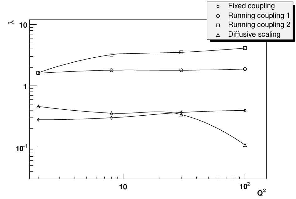
To study the $Q^{2}$ dependence of the fitted parameters and to quantify the amplitude of scaling violations, the data points are divided into four separate $Q^{2}$ samples: $[1;3]$, $[3;10]$, $[10;35]$, and $[35;150]$ GeV². The number of points in each region is similar (see table 3). The lower and upper bounds of $1$ GeV² and $150$ GeV² are chosen for the same reason as before. The $Q^{2}$ dependence of the parameter $\lambda$ is depicted in figure 10, and the fitted parameters together with the QF values are shown in table 3. There is a slight increase of the $\lambda$ parameter in the case of “Fixed Coupling” while “Running Coupling I” is quite flat. This can be easily understood since “Running Coupling I” shows a natural $Q^{2}$ evolution. We notice a stronger increase in the case of “Running Coupling II”, showing the breaking of this scaling as a function of $Q^{2}$. Since this scaling gives already the best QF, it would be worth to study the breaking of scaling and introduce it in the model to improve further the description of the data. The $\lambda$ parameter decreases strongly (especially in the last $Q^{2}$ bin) for the diffusive scaling. The fact that $\lambda$ depends strongly on $Q^{2}$ confirms the fact that this scaling leads to the worst description of the data.

Figure 9: $F_{2}$ data: Comparison of the QF for the different scaling as a function of $\lambda$. A $Q^{2}>3$ (left plot) or $Q^{2}>1$ (right plot) cut was applied to the data.

Figure 10: $F_{2}$ data: Variation of lambda as a function of $Q^{2}$ for the different scalings.

IV.4 Fits to DVCS data from H1 and ZEUS

After fitting all H1 and ZEUS $F_{2}$ data, it is worth studying whether the DVCS data measured by the same experiments [24] lead to the same results. The amount of data is smaller (34 points for H1 and ZEUS requiring $x\leq 0.01$ as for $F_{2}$ data) and the precision on the $\lambda$ parameter will be weaker. The kinematic coverage of the DVCS data covers a smaller region in $x$ and $Q^{2}$ as $F_{2}$: $4<Q^{2}<25$ GeV² and $5\cdot 10^{-4}<x<5\cdot 10^{-3}$. The results of the fits can be found in table 4 and Fig.11 and 12. The scaling results are displayed only for “Fixed Coupling” and “Running Coupling IIbis” since all plots look similar. To facilitate the comparison between the results of the fits to $F_{2}$ and DVCS data, a star is put in Fig. 12 at the position of the $\lambda$ value fitted to the H1+ZEUS $F_{2}$ data with $Q^{2}$ in the range $[3;150]$ GeV². We note that the DVCS data lead to similar $\lambda$ values to the $F_{2}$ data, showing the consistency of the scalings. The values of the QF show a tendency to favour fixed coupling, but all different scalings (even “Diffusive Scaling”) lead to reasonable values of QF.

Figure 11: DVCS data: Scaling curves for DVCS data and for “Fixed Coupling” and “Running Coupling IIbis”.

Figure 12: DVCS data: $\lambda$ dependence of the normalised QF to 1. for DVCS data and for “Fixed Coupling”, “Running Coupling I”, “Running Coupling II” and “Diffusive Scaling”. The star indicated the values of $\lambda$ obtained with a fit to $F_{2}$, $Q^{2}>3$ GeV². The values of $\lambda$ obtained in a fit to DVCS data are similar to te ones obtained in a fit to $F_{2}$ data.

V Implications for Diffraction and Vector Mesons

In this section, we check if the scalings found in the previous section can also describe diffractive and vector meson data. Since these data are much less precise than the $F_{2}$ or DVCS data and depend more on non-perturbative inputs (meson wave function, diffractive parton distribution inputs…), we choose to impose the same values of parameters found in the previous section and check if the scaling is also observed using this value. A fit to the diffractive data leads to large uncertainties on the parameter values since the number of data points is quite small and their uncertainties large.

Let us first describe the diffractive data. We use the latest $t$-integrated diffractive cross section measurements from H1 and ZEUS experiment [25], derived from the diffractive processes $e+p\rightarrow e+X+Y$, where the proton stays either intact or turns into a low mass state $Y$. The diffractive cross section in terms of the $t$-integrated reduced cross section $\sigma_{r}^{D(3)}(x_{I\!\!P},x,Q^{2})$ reads

$$\frac{d^{3}\sigma^{ep\rightarrow eXY}}{dx_{I\!\!P}dxdQ^{2}} = \frac{4\pi^{2}\alpha_{em}}{xQ^{4}}\left(1-y+\frac{y^{2}}{2}\right)\sigma_{r}^{D(3)}(x_{I\!\!P},x,Q^{2}),$$ (18)

$$\sigma_{r}^{D(3)} = F_{2}^{D(3)}-\frac{y^{2}}{1+(1-y)^{2}}F_{L}^{D(3)}.$$ (19)

The latter equation can be simplified to $\sigma_{r}^{D(3)}=F_{2}^{D(3)}$, since it is a very good approximation anywhere but at large $y$. H1 large rapidity gap measurements are realised with $M_{Y}<1.6$ GeV cut, whereas ZEUS measures with the $M_{Y}<2.3$ GeV cut using the $M_{X}$-method. Both experiments do not measure exactly the same cross section. However, the difference is a known constant factor; the ZEUS data points can be converted to the same $M_{Y}$ range as H1 by multiplying ZEUS values by factor of 0.85. In case of the $e+p\rightarrow e+X+p$ processes where the proton is tagged in Roman pot detectors (both H1 and ZEUS), the data points have to be multiplied by 1.23.

In order to test the geometrical scaling properties we plot the $\tau$ dependence of $\beta d\sigma_{diff}^{\gamma^{*}p\rightarrow Xp}/d\beta$, which can be expressed in terms of diffractive structure function as follows

$$\beta\frac{d\sigma_{diff}^{\gamma^{*}p\rightarrow Xp}}{d\beta}=\frac{4\pi^{2}\alpha_{em}}{Q^{2}}x_{I\!\!P}F_{2}^{D(3)}.$$ (20)

The definition of the $\tau$ variable is the same as in Table I replacing the variable $x$ by $x_{I\!\!P}$, $Q^{2}$ remaining the same.

In figure 13, we show the H1 and ZEUS diffractive data for $\beta d\sigma_{diff}^{\gamma^{*}p\rightarrow Xp}/d\beta$ as a function of the fixed coupling scaling variable $\tau$ for six different fixed values of $\beta$: 0.04, 0.1, 0.2, 0.4, 0.65, and 0.90. Only the data points in the $Q^{2}$ region $[5;90]$ GeV² and with $x_{I\!\!P}<0.01$ are plotted. The restriction to the mentioned fixed values implies that the data set is dominated by H1 data. We just give in Fig. 13 the results for “Fixed Coupling” since the other scalings give similar results which are not distinguishable given the large uncertainties on $F_{2}^{D}$. The parameters fitted to the H1 and ZEUS $F_{2}$ data are used to make the prediction on $F_{2}^{D}$. Up to $\beta=0.65$ (the first five bins), the data points lie on a unique curve and thus confirm the geometrical scaling prediction. The data points at the highest $\beta$ values (low masses) are more sensitive to low mass resonances and are not expected to show a perfect scaling. The values of the QF are also given in Table 5. In many bins, “Running Coupling IIbis” gives the best QF.

Following the Ingelman-Schlein model of the Pomeron, we also tested the scaling in $\beta$, $Q^{2}$ in the diffraction data. The definition of the $\tau$ variable is the same as in Table I replacing the variable $x$ by $\beta$, $Q^{2}$ remaining the same. Figure 14 presents the H1 and ZEUS diffractive data in the same $Q^{2}$ region with $\beta<0.5$ at five different fixed values of $x_{I\!\!P}$: 0.0003, 0.001, 0.003, 0.01, and 0.03. The restriction to these fixed values results in favouring the H1 LRG data. Similarly as in the previous case, the parameter values from the fit to H1 and ZEUS $F_{2}$ data are used. The scaling is definitely not as good as the one for a fixed $\beta$.

The fits to H1 and ZEUS $F_{2}$ data are also tested on vector meson data from both experiments [26]. Note the scale $M_{V}^{2}$ present in the scaling function in (12). The definition of the $\tau$ variable is the same as in Table I replacing the variable $Q^{2}$ by $Q^{2}+M_{V}^{2}$ $M_{V}^{2}$ being the mass of the vector meson, $x$ remaining the same. The QFs are given in table 6 and scaling curves for “Fixed Coupling” are given in Fig. 15. We only show the results for “Fixed Coupling” since all scalings give similar results. We see that the scaling is indeed verified for $\rho$, $J/\Psi$, and $\phi$ and the data points show a tendency to be more dispersed for $\phi$. Interestingly enough, “Diffusive Scaling” leads to the best QF.

Figure 13: $F_{2}^{D}$ data: Scaling curves obtained for fixed values of $\beta$ for $F_{2}^{D}$ and fixed coupling. The parameters are fixed to the values obtained with a fit to $F_{2}$ data with $Q^{2}>3$ GeV².

Figure 14: $F_{2}^{D}$ data: Scaling curves obtained for fixed values of $x_{I\!\!P}$ for $F_{2}^{D}$ and “Fixed Coupling”. The parameters are fixed to the values obtained with a fit to $F_{2}$ data with $Q^{2}>3$ GeV².

Figure 15: Vector meson data: Scaling curves obtained for fixed values of $x_{I\!\!P}$ and for “Fixed Coupling”, for vector meson data. The parameters are fixed to the values obtained with a fit to $F_{2}$ data with $Q^{2}>3$ GeV².

VI Conclusions

In this paper we analysed the scaling properties of deep inelastic observables such as the total cross section, DVCS, vector meson production, and the diffractive cross section, using all available low x data, i.e. from the H1 [20], ZEUS [21], NMC [22] and E665 [23] experiments. In order to be as model independant as possible, we used the quality factor method [12], allowing to test the validity of scaling variables without any assumption concerning the shape of the scaling function. Four scaling variables (1-4), motivated by various approximations of QCD high energy evolution, were considered, including the new “Running Coupling II” one derived in [6]. Different versions of those scalings were tested, setting the rapidity shift $Y_{0}$ to $0$ and the reference scale $\Lambda$ to either $0.2$ GeV or to $1$ GeV, or taking $\Lambda$ and $Y_{0}$ as free parameters to be fitted.

We showed that the “Fixed Coupling”, “Running Coupling I” and “Running Coupling II” scaling variables lead to a good scaling behavior of the total cross section from the $F_{2}$ data, with similar quality factors. The “Diffusive scaling” is disfavoured compared to them. More precisely, the “Running Coupling IIbis”, with the free parameters $Y_{0}$ and $\Lambda$, gives the best scaling behavior in the range $3$ GeV${}^{2}<Q^{2}<150$ GeV² and $x<0.01$, with reasonnable values of $Y_{0}$ and $\Lambda$ extracted from the fit of the quality factor. The “Fixed Coupling” scaling is less deteriorated than the “Running Coupling II” scaling when one adds the points with $1$ GeV${}^{2}<Q^{2}<3$ GeV² to the fit, which corresponds to the boundary of the validity range of the perturbative scaling predictions. Dividing the data in four $Q^{2}$ bins, we also studied the $Q^{2}$ dependence of the optimal value for the $\lambda$ parameter. “Running Coupling I” gives the most stable values and “Diffusive scaling” the less stable, and “Running Coupling II” gives stable values except at low $Q^{2}$.

The quality factors of the scaling variables were fitted independantly on the DVCS data, and give similar results as on the total cross section. In particular, for each scaling variable, the values of the parameter $\lambda$ obtained from the fit in the two cases are very close.

We used the values of the parameters obtained from a fit to $F_{2}$ data to test the various scaling variables on the diffractive cross section and vector meson production data. For the former observable we tested both the fixed $\beta$ scaling behavior in $x_{I\!\!P}$ and the fixed $x_{I\!\!P}$ scaling behavior in $\beta$. At fixed $\beta$, we found a scaling behavior up to $\beta=0.65$. For most $\beta$ bins the best results are given by “Running Coupling ” scaling variables, and the “Diffusive scaling” is often disfavoured.

At fixed $x_{I\!\!P}$, the scaling behavior of the diffractive cross section as a function of $\beta$ and $Q^{2}$ is far less obvious. This is not a surprise, as not enough data is available in the genuine small $\beta$ region. A tendency of scaling is however observed for the $x_{I\!\!P}=0.03$ bin.

Concerning $\rho$, $J/\Psi$, and $\phi$ production, we found a reasonable scaling behavior for all tested scaling variables, with the hard scale $Q^{2}+M_{V}^{2}$, borrowed from vector mesons wave function studies. Surprisingly, the best scaling is for all three vector mesons the “Diffusive scaling”.

As a phenomenological outlook, it seems useful to work out models dipole amplitude wich could incorporate the successful scaling laws following the example of e.g. the Iancu Itakura Munier model [27]. The quality factor method is a good tool to detect the scaling properties of data, and can guide the formulation of models with good $\chi^{2}$. Our study is a good incentive for the formulation of appropriate models with running coupling scaling. There exists phenomenological models based on fixed coupling diffusive scaling [28]. The test of scaling and the formulation of model will be important to analyse future LHC data. In particular, the wider kinematical range open by the LHC could help disentangling the scaling laws in competition, or reveal a new scaling (such as the diffusive one) at higher energies.

On the theoretical ground, our phenomenological analysis can help to improve the theoretical analysis of scaling. Indeed, a mere comparison between the values of $\lambda$ and the corresponding prediction based on the leading order BFKL kernel shows that one should go beyond this approximation to get an agreement. Thus, our determination of the basic scaling parameters can help the theoretical QCD analysis.

$Q^{2}$	data	$n_{points}$	FC	RC I	RC II	RC II bis	DS
$Q^{2}\geq 3$	all data	217	$\lambda$=0.330	$\lambda$=1.841	$\lambda$=3.436	$\lambda$=3.905	$\lambda$=0.362
						$Y_{0}$=-1.200
						$\Lambda=0.300$
			$QF$=1.63	$QF$=1.62	$QF$=1.69	$QF$=1.82	$QF$=1.44
$Q^{2}\geq 3$	H1	87	$\lambda$=0.331	$\lambda$=1.736	$\lambda$=3.228	$\lambda$=4.891	$\lambda$=0.311
						$Y_{0}$=-2.516
						$\Lambda=0.351$
			$QF$=5.72	$QF$=5.88	$QF$=5.79	$QF$=6.31	$QF$=5.28
$Q^{2}\geq 3$	ZEUS	127	$\lambda$=0.368	$\lambda$=1.809	$\lambda$=3.395	$\lambda$=4.327	$\lambda$=0.366
						$Y_{0}$=-1.917
						$\Lambda=0.203$
			$QF$=3.03	$QF$=3.08	$QF$=3.00	$QF$=3.28	$QF$=2.32
$Q^{2}\geq 3$	H1$+$ZEUS	214	$\lambda$=0.379	$\lambda$=1.839	$\lambda$=3.436	$\lambda$=4.147	$\lambda$=0.321
						$Y_{0}$=-1.182
						$\Lambda=0.333$
			$QF$=1.99	$QF$=1.76	$QF$=1.83	$QF$=2.02	$QF$=1.54
$Q^{2}\geq 1$	all data	308	$\lambda$=0.321	$\lambda$=1.700	$\lambda$=2.932	$\lambda$=3.154	$\lambda$=0.369
						$Y_{0}$=-0.199
						$\Lambda=0.440$
			$QF$=1.30	$QF$=1.20	$QF$=1.07	$QF$=1.27	$QF$=1.02
$Q^{2}\geq 1$	H1	135	$\lambda$=0.314	$\lambda$=1.710	$\lambda$=3.073	$\lambda$=3.159	$\lambda$=0.353
						$Y_{0}$=-0.367
						$\Lambda=0.201$
			$QF$=3.43	$QF$=3.56	$QF$=3.51	$QF$=3.52	$QF$=2.79
$Q^{2}\geq 1$	ZEUS	147	$\lambda$=0.358	$\lambda$=1.809	$\lambda$=3.331	$\lambda$=3.747	$\lambda$=0.313
						$Y_{0}$=1.290
						$\Lambda=0.060$
			$QF$=3.28	$QF$=3.20	$QF$=3.05	$QF$=3.29	$QF$=2.22
$Q^{2}\geq 1$	H1$+$ZEUS	282	$\lambda$=0.368	$\lambda$=1.797	$\lambda$=3.226	$\lambda$=3.918	$\lambda$=0.367
						$Y_{0}$=-1.201
						$\Lambda=0.225$
			$QF$=1.69	$QF$=1.71	$QF$=1.61	$QF$=1.74	$QF$=1.32

Table 2: $F_{2}$ data: QF (multiplied by $10^{3}$) and pamameters of the fixed coupling, running coupling I and II, and diffusive scalings for the different data sets. We distinguish the data sets for $Q^{2}>3$ and $Q^{2}>1$ GeV², and we compare the fit results using the full data set, or the H1 or ZEUS data only.

$Q^{2}$	$n_{points}$	FC	RC I	RC II	DS
$1\leq Q^{2}\leq 3$	91	$\lambda$=0.279	$\lambda$=1.603	$\lambda$=1.627	$\lambda$=0.461
		$QF$=0.594	$QF$=0.575	$QF$=0.600	$QF$=0.571
$3<Q^{2}\leq 10$	98	$\lambda$=0.301	$\lambda$=1.800	$\lambda$=3.219	$\lambda$=0.357
		$QF$=0.584	$QF$=0.544	$QF$=0.547	$QF$=0.526
$10<Q^{2}\leq 35$	86	$\lambda$=0.367	$\lambda$=1.794	$\lambda$=3.521	$\lambda$=0.340
		$QF$=3.53	$QF$=3.06	$QF$=3.22	$QF$=2.67
$35<Q^{2}\leq 150$	53	$\lambda$=0.397	$\lambda$=1.877	$\lambda$=4.135	$\lambda$=0.108
		$QF$=8.33	$QF$=8.00	$QF$=8.26	$QF$=6.37

Table 3: $F_{2}$ data: $\lambda$ dependence as a function of $Q^{2}$ - The QF are multiplied by $10^{3}$ for simplification.

$n_{points}$	FC	RC I	RC II	RC II bis	DS
34	$\lambda$=0.361	$\lambda$=1.829	$\lambda$=3.481	$\lambda$=5.717	$\lambda$=0.335
				$Y_{0}$=-1.89
				$\Lambda=0.01$
	$QF$=3.75	$QF$=3.62	$QF$=3.24	$QF$=3.52	$QF$=3.38

Table 4: DVCS data: Values of QF (multiplied by $10^{3}$) and fit parameters for the different scalings. The paramters obtained for all scaling (except “Running Coupling IIbis”) are close to those found for $F_{2}$ (see Table II). We note that the small amount of data lead to a bad precision of the fit for “Running Coupling IIbis” when three parameters are used.

$\beta$	$n_{points}$	FC	RC I	RC II	RC II bis	DS
0.04	14	2.54	2.80	2.91	3.02	1.64
0.1	30	0.610	0.579	0.600	0.605	0.660
0.2	40	0.951	1.13	1.20	1.46	1.14
0.4	64	1.05	0.952	0.984	0.998	1.00
0.65	60	1.34	1.47	1.93	1.35	1.20
0.9	59	0.380	0.510	0.572	0.492	0.372

Table 5: $F_{2}^{D}$ data: Values of QF (multiplied by $10^{3}$) for the different scalings. The parameters $\lambda$, $Y_{0}$ and $\Lambda$ are fixed to the values obtained in the fits to $F_{2}$ data. Cuts on data $x_{I\!\!P}<0.01$, $5\leq Q^{2}\leq 90$ were applied.

VM	$n_{points}$	FC	RC I	RC II	RC II bis	DS
$J/\psi$	28	2.16	1.83	1.88	1.93	2.50
$\rho$	62	1.02	0.814	0.803	0.964	1.28
$\phi$	28	1.95	2.44	2.41	3.17	3.18

Table 6: Vector mesons data: Values of QF (multiplied by $10^{3}$) for the different scalings. The parameters $\lambda$, $Y_{0}$ and $\Lambda$ are fixed to the values obtained in the fits to $F_{2}$ data.

References

- [1] A. M. Staśto, K. Golec-Biernat, and J. Kwiecinski, Phys. Rev. Lett. 86, 596 (2001).
- [2] K. Golec-Biernat and M. Wusthoff, Phys. Rev. D 59, 014017 (1999).
- [3] A.H. Mueller, “Parton saturation: An overview”, [arXiv:hep-ph/0111244].
- [4] I. Balitsky, Nucl. Phys. B 463, 99 (1996); Y. V. Kovchegov, Phys. Rev. D 60, 034008 (1999), D 61, 074018 (2000).
- [5] S. Munier and R. Peschanski, Phys. Rev. Lett. 91, 232001 (2003), Phys. Rev. D69, 034008 (2004), D 70, 077503 (2004).
- [6] G. Beuf, arXiv:0803.2167 [hep-ph].
- [7] E. Iancu, K. Itakura and L. McLerran, Nucl. Phys. A 708, 327 (2002); A. H. Mueller and D. N. Triantafyllopoulos, Nucl. Phys. B 640, 331 (2002); D. N. Triantafyllopoulos, Nucl. Phys. B 648, 293 (2003).
- [8] L. N. Lipatov, Sov. J. Nucl. Phys. 23, 338 (1976); E. A. Kuraev, L. N. Lipatov, and V. S. Fadin, Sov. Phys. JETP 45, 199 (1977), I. I. Balitsky and L. N. Lipatov, Sov. J. Nucl. Phys. 28, 822 (1978).
- [9] E. Iancu, A. H. Mueller and S. Munier, Phys. Lett. B 606, 342 (2005) [arXiv:hep-ph/0410018]; Y. Hatta, E. Iancu, C. Marquet, G. Soyez and D. N. Triantafyllopoulos, Nucl. Phys. A 773, 95 (2006) [arXiv:hep-ph/0601150].
- [10] C. Marquet and L. Schoeffel, Phys. Lett. B 639, 471 (2006) [arXiv:hep-ph/0606079].
- [11] G. Ingelman and P. E. Schlein, Phys. Lett. B 152, 256 (1985).
- [12] F. Gelis, R. Peschanski, G. Soyez and L. Schoeffel, Phys. Lett. B 647, 376 (2007) [arXiv:hep-ph/0610435].
- [13] V. S. Fadin and L. N. Lipatov, Phys. Lett. B 429, 127 (1998); M. Ciafaloni and G. Camici, Phys. Lett. B 430, 349 (1998).
- [14] G. P. Salam, JHEP 07, 019 (1998).
- [15] M. Ciafaloni, D. Colferai, and G. P. Salam, Phys. Rev. D 60, 114036 (1999).
- [16]
R. Peschanski, C. Royon and L. Schoeffel,
Nucl. Phys. B 716, 401 (2005);
O. Kepka, C. Marquet, R. Peschanski and C. Royon, Phys. Lett. B 655, 236 (2007); Eur. Phys. J. C 55, 259 (2008). - [17] L. V. Gribov, E. M. Levin and M. G. Ryskin, Phys. Rept. 100 (1983) 1.
- [18] A. Dumitru, E. Iancu, L. Portugal, G. Soyez and D. N. Triantafyllopoulos, JHEP 0708, 062 (2007) [arXiv:0706.2540 [hep-ph]].
- [19] Y. V. Kovchegov and H. Weigert, Nucl. Phys. A 784 (2007) 188 [arXiv:hep-ph/0609090]; I. Balitsky, Phys. Rev. D 75, 014001 (2007) [arXiv:hep-ph/0609105]; I. Balitsky and G. A. Chirilli, Phys. Rev. D 77, 014019 (2008) [arXiv:0710.4330 [hep-ph]].
- [20] C. Adloff et al. [H1 Collaboration], Eur. Phys. J. C 21 (2001) 33 [arXiv:hep-ex/0012053]; Eur. Phys. J. C 30 (2003) 1 [arXiv:hep-ex/0304003].
- [21]
J. Breitweg et al. [ZEUS Collaboration],
Eur. Phys. J. C 7 (1999) 609 [arXiv:hep-ex/9809005];
Phys. Lett. B 487 (2000) 273 [arXiv:hep-ex/0006013];
S. Chekanov et al. [ZEUS Collaboration],
Eur. Phys. J. C 21 (2001) 443 [arXiv:hep-ex/0105090].
Phys. Rev. D 70 (2004) 052001 [arXiv:hep-ex/0401003].
The data in the last ZEUS paper include contributions for and but those can be neglected within the kinematical domain we consider. - [22] M. Arneodo et al. [New Muon Collaboration], Nucl. Phys. B 483 (1997) 3 [arXiv:hep-ph/9610231].
- [23] M. R. Adams et al. [E665 Collaboration], Phys. Rev. D 54 (1996) 3006.
- [24] A. Aktas et al. [H1 Collaboration], Phys. Lett. B659 (2008) 796-806 A. Aktas et al. [H1 Collaboration], Eur. Phys. J. C 44 (2005) 1-11 [arXiv:hep-ex/0505061]
- [25] A. Aktas et al. [H1 Collaboration], Eur. Phys. J. C 48 (2006) 715-748 [arXiv:hep-ex/0606004] S. Chekanov et al. [ZEUS Collaboration], Nucl. Phys. B 713 (2005) 3-80 S. Chekanov et al. [ZEUS Collaboration], Eur. Phys. J. C 38 (2004) 43-67
- [26] S. Chekanov et al. [ZEUS Collaboration], Nucl. Phys. B 718 (2005) 3-31 A. Aktas et al. [H1 Collaboration], Eur. Phys. J. C 46 (2006) 585-603 [arXiv:hep-ex/0510016] A. Aktas et al. [H1 Collaboration], Eur.Phys.J. C 13 (2000) 371-396 [arXiv:hep-ex/9902019]
- [27] E. Iancu, K. Itakura and S. Munier, Phys. Lett. B 590 (2004) 199 [arXiv:hep-ph/0310338].
- [28] M. Kozlov, A. Shoshi and W. Xiang, JHEP 0710 (2007) 020 [arXiv:0707.4142 [hep-ph]].