Relation between chiral symmetry breaking and confinement in YM-theories

Abstract

Spectral sums of the Dirac-Wilson operator and their relation to the Polyakov loop are thoroughly investigated. The approach by Gattringer is generalized to mode sums which reconstruct the Polyakov loop locally. This opens the possibility to study the mode sum approximation to the Polyakov loop correlator. The approach is rederived for the ab initio continuum formulation of Yang-Mills theories, and the convergence of the mode sum is studied in detail. The mode sums are then explicitly calculated for the Schwinger model and $SU(2)$ gauge theory in a homogeneous background field. Using $SU(2)$ lattice gauge theory, the IR dominated mode sums are considered and the mode sum approximation to the static quark antiquark potential is obtained numerically. We find a good agreement between the mode sum approximation and the static potential at large distances for the confinement and the high temperature plasma phase.

I Introduction

Color confinement and spontaneous chiral symmetry breaking are the two most relevant features of Yang-Mills theory when the structure of matter under normal conditions is explored. Both phenomenons are attributed to the low energy sector of Yang-Mills theory, an analytic description of which is hardly feasible due to strong couplings between the basic degrees of freedom, quarks and gluons. Lattice gauge simulations found that both so different phenomenons are intimately related: in the chiral limit, the critical temperature for deconfinement $T_{d}$ and the critical temperature for chiral restoration $T_{c}$ coincide [1]. This finding is highly nontrivial since the expectations had been that two totally different mechanisms involving different energy scales were at work for each phenomenon. Indeed, if quarks which transform under the adjoint representation were considered instead of the quark fields of standard QCD, largely different values for $T_{d}$ and $T_{c}$ were reported in [2].

These results have stirred the hope that a single low energy effective degree of freedom is responsible for both phenomenons. Given that in pure $SU(N)$ gauge theory the long distance part of the static quark potential depends on the $N$-ality of the quarks and that the crucial difference between fundamental and adjoint quarks is $N$-ality again, center vortices appear as a natural candidate for such a degree of freedom: these vortices are tightly related to confinement, are sensible in the continuum limit and offer an intriguing picture of deconfinement at high temperatures [3, 4, 5, 6]. It was found quite recently that the vortices extend their reach to a description of spontaneous chiral symmetry breaking as well [7].

In order to reveal a model independent link between confinement and chiral symmetry breaking, Gattringer proposed to reconstruct the Polyakov loop expectation value $\langle P\rangle$ in terms of a particular spectral function ${\mathcal{S}}_{N_{t}}$ of the lattice Dirac operator [8]. While the low lying modes of the Dirac operator are directly related to chiral symmetry breaking by virtue of the Banks-Casher relation, the Polyakov loop expectation value serves as the litmus paper for confinement. Spectral representations of $\langle P\rangle$ have subsequently been the subject of recent studies. Bruckmann et al. [9] investigated the response of the eigenvalues of the staggered Dirac operator to a twist of the boundary conditions. They found that the infrared part of the spectrum is most sensitive to twists. It was subsequently pointed out that the spectral sum ${\mathcal{S}}_{N_{t}}$, originally proposed by Gattringer, is dominated by the ultraviolet part of the spectrum since the sum contains large powers of the eigenvalues [8, 9, 10, 11]. A sensible continuum limit was caught into question. In [10] alternative spectral sums were put forward which serve as order parameters for confinement and which receive their main contributions from the infrared part of the spectrum. One of these sums is of particular interest since it relates the dressed Polyakov loops to the chiral condensate via the celebrated Banks-Casher relation [12]. If one twists the gauge field by a complex number $z$ with unit modulus (or equivalently twists the boundary conditions by $1/z$) and picks the coefficient of $z^{k}$ in the spectral sums one obtains the dressed Polyakov loops with winding number $k$ [10]. With this method Bilgici et al. [13] connect the eigenvalue density at zero and therefore the chiral condensate to the dressed Polyakov loops. Numerical results for spectral sums of various lattice Dirac operators with quenched configurations can be found in the recent papers [9, 10, 12, 14] and for ensembles generated with dynamical fermions in [11]. We finally point out that the spectral approach to the Polyakov line has been extended by using eigenmodes of the Laplacian operator [15]. There, the spectral sum acts as gauge invariant low energy filter which reveals the “classical” texture while quark confinement is still active.

In this paper, we generalize the concept of the mode sum approximation to reconstruct the Polyakov loop locally. This has the great advantage that now the Polyakov loop correlator and the static quark antiquark potential can be studied in the light of a few low lying modes of the Dirac operator. We then point out that the mode sum approach is not solely tied to lattice quark operators and present an explicit construction of this approach in the ab initio continuum formulation of Yang-Mills theory. The convergence of the mode sums for all polynomial functions of the continuum Dirac operator is demonstrated for the first time. We then argue that a wide class of IR dominated mode sums are in fact proportional to the Polyakov loop. This conjecture is fostered by an explicit calculation of these mode sums for Schwinger model and for $SU(2)$ gauge theory with constant background field strength. We then consider $SU(2)$ gauge theory above and below the deconfinement temperature by means of lattice gauge simulations. Most important, we find that a few low lying modes of the quark operator are sufficient to reconstruct the static quark potential at large quark antiquark distances. This is a gauge invariant and model independent signal that the color confinement mechanism has its fingerprints in the low lying quark spectrum.

II Recall of spectral sums for Lattice models

The $j$-th power of a Dirac operator ${\mathcal{D}}_{U}$ with nearest neighbor interaction on an Euclidean lattice with $N_{t}\times N_{s}^{d-1}$ sites can be expanded in Wilson loops of length up to $j$,

$$\langle x|{\mathcal{D}}_{U}^{\,j}|x\rangle=\sum_{|{\mathcal{C}}_{x}|\leq j}a_{{\mathcal{C}}_{x}}{\mathcal{W}}_{{\mathcal{C}}_{x}}.$$ (1)

The value of the coefficient $a_{{\mathcal{C}}_{x}}$ multiplying the holonomy ${\mathcal{W}}_{{\mathcal{C}}_{x}}$ of the loop ${\mathcal{C}}_{x}$ with base $x$ depends on the type of fermions under consideration. The expansion (1) is used to relate the Polyakov loop

$$P(\boldmathe{x})=\tr{\mathcal{P}}(\boldmathe{x}),\quad{\mathcal{P}}(\boldmathe{x})=\prod_{x_{0}}U_{0}(x_{0},\boldmathe{x})$$ (2)

with the spectrum of the Dirac operator [8]. On a lattice with $N_{s}\gg N_{t}$ the sum on the right hand side of (1) contains contractable loops and loops winding once or several times around the torus in time direction. In order to relate the Polyakov loop to spectral sums of quark eigenmodes an interface is inserted into the lattice gauge configuration $U_{\mu}(x),\;x=(x_{0},\boldmathe{x})$ by

$${{}^{z}}U_{\mu}(x_{0},\boldmathe{x})=\left\{\begin{array}[]{cl}z\cdot U_{0}(x_{0},\boldmathe{x})&\hbox{ for $\mu=0$ and $x_{0}=0$ }\\ U_{\mu}(x_{0},\boldmathe{x})&\hbox{ otherwise },\\ \end{array}\right.$$ (3)

where $z=e^{2\pi i\alpha}$ is a center element. Contractable Wilson loops are invariant when one inserts an interface which is referred to as twisting the gauge field. Wilson loops winding $k$-times acquire a factor $z^{k}$. It follows that for a twisted gauge field the coefficient of $z$ in the series (1) becomes a linear combination of dressed Polyakov loops passing through $x$, having length $\leq j$ and winding $1+kN$ times around the time direction. Here $k$ is an integer and $z^{N}=1$. For $j=N_{t}$ there is only one such loop, namely the straight Polyakov loop at $\boldmathe{x}$. After taking the traces over spinor and color-indices the sum over $x^{0}$ yields [8]

$$P(\boldmathe{x})=\frac{1}{\kappa}\sum_{k=1}^{N}z_{k}^{\ast}\sum_{p=1}^{n_{p}}{{}^{z_{k}}\!\varrho}_{p}(\boldmathe{x})\,\left({{}^{z_{k}\!}\lambda}_{p}\right)^{N_{t}},$$ (4)

$${{}^{z}\!\varrho}_{p}(\boldmathe{x})=\sum_{x_{0}=1}^{N_{t}}{{}^{z}\!\varrho}_{p}(x^{0},\boldmathe{x}).$$ (5)

The first sum in (4) is over all center elements $z_{1},\dots,z_{N}$ and the second over all $n_{p}$ eigenvalues of the Dirac operator. The value of the constant $\kappa$ depends on the type of lattice Dirac operator under consideration. ${{}^{z}\!\varrho}_{p}(x)$ is the eigenvalue density and ${{}^{z\!}\lambda}_{p}$ the $p$-th eigenvalue of the Dirac operator ${}^{z}{\mathcal{D}}_{U}\equiv{\mathcal{D}}_{{}^{z}U}$ with $z$-twisted gauge field,

$$\begin{split}(^{z}{\mathcal{D}}_{U})\,&{{}^{z}}\psi_{p}={{}^{z\!}\lambda}_{p}{{}^{z}}\psi_{p}\quad\hbox{{with}}\quad\\ &{{}^{z}}\psi_{p}(x_{0}+N_{t},\boldmathe{x})=-{{}^{z}}\psi_{p}(x_{0},\boldmathe{x}).\end{split}$$ (6)

In terms of the normalized eigenmodes the color-blind density reads

$${{}^{z}\!\varrho}_{p}(x)=\sum_{\ell}\left|{{}^{z}}\psi_{p,\ell}(x)\right|^{2},$$ (7)

where the sum extends over all eigenfunctions of ${}^{z}{\mathcal{D}}_{U}$ with fixed energy $\lambda_{p}$. The densities ${{}^{z}\!\varrho}_{p}$ are gauge invariant scalar fields. For the trivial center element $z=1$ we often write $\,\varrho$ instead of ${{}^{z}\!\varrho}$. Averaging the local identity (4) over space yields

$$\bar{P}\equiv\frac{1}{V_{s}}\sum{x}P(\boldmathe{x})=\frac{1}{\kappa}\sum_{k}z_{k}^{\ast}\sum_{p}\left({{}^{z_{k}\!}\lambda}_{p}\right)^{N_{t}}.$$ (8)

This simple formula for the averaged loop has been investigated a lot in the past. The main problem with the sum on the right hand side is that it is dominated by the ultraviolet part of the spectrum and therefore is expected to have an ill defined continuum limit. But all spectral sums of the form

$$\begin{split}{\mathcal{S}}_{f}(U)&=\sum_{k}z_{k}^{\ast}\sum_{p}f({{}^{z_{k}\!}\lambda}_{p})=\sum_{x}{\mathcal{S}}_{f}(U;x)\\ {\mathcal{S}}_{f}(U;x)&=\sum_{k}z_{k}^{\ast}\sum_{p=1}^{n_{p}}{{}^{z_{k}}\!\varrho}_{p}(x)\,f({{}^{z_{k}\!}\lambda}_{p})\,\end{split}$$ (9)

define (nonlocal) order parameters for the center symmetry [10]. Indeed, if we twist the gauge field with a center element $z$, we obtain:

$${\mathcal{S}}_{f}(^{z}U)=z{\mathcal{S}}_{f}(U).$$ (10)

Our important observation is that, as the Polyakov loop, all spectral sums pick up a factor in the center of the group. Thus, not only the Polyakov loop, but also any other spectral sum of the above type might serve as a litmus paper for confinement. Of particular interest are sums which get their main contribution from the low lying eigenvalues. It has been convincingly demonstrated in [10] that the Gaussian sum with $f({\mathcal{D}})=\exp(-{\mathcal{D}}{\mathcal{D}}^{\,\dagger})$ is very well suited for that purpose. For a $SU(3)$ lattice gauge theory, Figure 1 shows the Monte-Carlo averages of the partial sums

$${\mathcal{G}}_{n}(U)=\sum_{k=1}^{3}z_{k}^{\ast}\sum_{p=1}^{n}\exp\left(-|{{}^{z_{k}\!}\lambda}_{p}|^{2}\right)$$ (11)

and demonstrates their rapid convergence to a multiple of the (rotated) Polyakov loop expectation value. Actually it is sufficient to include less than $5\%$ of the low lying eigenvalues to obtain a decent approximation of the limiting value.

Figure 1: Mean Gaussian sums ${\mathcal{G}}^{\rm rot}_{n}$ for $SU(3)$ on a $4^{3}\!\times\!3$-lattice near $\beta_{\rm crit}$. The graphs are labeled with $\beta$.

Similar results hold for the spectral sums of the functions $f({\mathcal{D}})={\mathcal{D}}^{\,-1}$ and $f({\mathcal{D}})={\mathcal{D}}^{\,-2}$ corresponding to the propagators of ${\mathcal{D}}$ and ${\mathcal{D}}^{2}$. They are of particular interest since they relate to the celebrated Banks-Casher relation.

The spectral problem (6) is gauge-equivalent to the problem with twisted boundary conditions

$$\begin{split}{\mathcal{D}}_{U}&{{}^{z}}\psi_{p}={{}^{z\!}\lambda}_{p}{{}^{z}}\psi_{p}\quad\hbox{{with}}\quad\\ &{{}^{z}}\psi_{p}(x_{0}+N_{t},\boldmathe{x})=-z^{\ast}\,{{}^{z}}\psi_{p}(x_{0},\boldmathe{x}).\end{split}$$ (12)

For calculating the gauge invariant spectral sums we may either twist the gauge field as in (3) or twist the boundary conditions as in (12). Bilgici et al. extended the results in [10] and allowed for twists of the type $z=\exp(2\pi i\alpha)$ in the boundary conditions [13]. Admitting arbitrary values $\alpha\in[0,1[$, the twists are no longer center elements of $SU(N)$ but only of $U(N)$. Using nevertheless (12) as the primary definition of twist when $z$ is extended to $U(1)$ phases, the coefficients $\tilde{\Sigma}_{n}$ of the expansion of the twisted quark propagator in powers of $z$ can be easily obtained [13]. The coefficient $\tilde{\Sigma}_{n}$ can be written as sums over all loops winding $n$-times around the torus in time direction. In particular, the coefficient $\tilde{\Sigma}_{1}$ is related to the spacetime integrated spectral density ${{}^{z}\!\varrho}(\lambda)$ for vanishing eigenvalue by

$$\tilde{\Sigma}_{1}=\int_{0}^{1}d\alpha\;z^{\ast}\cdot{{}^{z}\!\varrho}(\lambda\searrow 0),\quad z=e^{2\pi i\alpha}.$$ (13)

In the numerical investigation below we will focus on truncations of local spectral sums (9). We will use IR sensitive spectral sums to find good approximations to $\langle P(\boldmathe{x})P(\boldmathe{y})\rangle$ or higher correlators. Guided by our previous results we consider the partial Gaussian sums

$${\mathcal{G}}_{n}(U;\boldmathe{x})=\sum_{k}z^{\ast}_{k}\sum_{p=1}^{n}\!{{}^{z_{k}}\!\varrho}_{p}(\boldmathe{x})\;\exp\left(-|{{}^{z_{k}\!}\lambda}_{p}|^{2}\right),$$ (14)

where $\varrho_{p}(\boldmathe{x})$ has been introduced in (5) and (7). We will study by analytical (for cases which admit a complete analytical evaluation of the spectral sums) and by numerical means whether and, in case, to which extent the correlator of two partial sums approaches the Polyakov loop correlator

$$\langle{\mathcal{G}}_{n}(U;\boldmathe{x}){\mathcal{G}}_{n}(U;\boldmathe{y})\rangle\longrightarrow\hbox{const}\cdot\langle P(\boldmathe{x})P(\boldmathe{y})\rangle,$$ (15)

when $n$ tends to the total number $n_{p}$ of eigenvalues.

III Spectral Sums and Center Symmetry in the Continuum

So far the intriguing relations between spectral sums of twisted configurations and Polyakov loops have been established for lattice regulated gauge theories only. It is yet an open question which results remain meaningful in the continuum limit. Clearly, an object like $\Tr({\mathcal{D}}_{U}^{N_{t}})$ does not make sense in the continuum, and this was the main motivation in [10] to introduce the generalized spectral sums (9). Even if $\,\Tr f({\mathcal{D}})$ exists in the continuum limit and even if, on the lattice,

$${\mathcal{S}}_{f}(U;\boldmathe{x})=\sum_{x^{0}}{\mathcal{S}}_{f}(x^{0},\boldmathe{x};U)$$ (16)

with ${\mathcal{S}}_{f}(x;U)$ from (9) is roughly proportional to the Polyakov loop, there are still the possibilities that this approximate proportionality is lost in the continuum limit or that the constant of proportionality diverges. For example, it was observed that the factor $\kappa$ in (4) diverges in the continuum limit.

In this section we study spectral sums for Euclidean gauge theories in the ab initio continuum formulation for a torus of extend $\beta\times L^{d-1}$ with $L$ much bigger than the inverse temperature $\beta=1/k_{B}T$. The volume of the torus is $V=\beta\cdot V_{s}$ while the spatial volume is given by $V_{s}=L^{d-1}$. On a torus the continuum Dirac operator

$${\mathcal{D}}_{A}=i\gamma^{\mu}(\partial_{\mu}-iA_{\mu})+im$$ (17)

has discrete eigenvalues $\lambda_{p}$ which are real for a vanishing quark mass. We shall consider Hermitian vector potentials

$$A_{\mu}=A^{a}_{\mu}\lambda^{a}.$$ (18)

The gauge field is described by real-valued functions $A^{a}_{\mu}(x)$ (with $a\in\{1,2,\dots,\dim(G)\}$) of the Euclidean space-time points $x=(x_{0},\boldmathe{x})$. The path integral measure contains fields that obey periodic boundary conditions in the Euclidean time direction,

$$A_{\mu}(x_{0}+\beta,\boldmathe{x})=A_{\mu}(x_{0},\boldmathe{x}).$$ (19)

Even for configurations with nonvanishing instanton number we may assume periodicity in the time direction [16, 17]. The Yang-Mills action is invariant under gauge transformations

$${}^{g}\hskip-1.99168ptA_{\mu}=g(A_{\mu}+i\partial_{\mu})g^{-1},\quad g(x)\in G,$$ (20)

under which the field strength transforms as ${}^{g}\hskip-1.13809ptF_{\mu\nu}=gF_{\mu\nu}g^{-1}.$ In order to maintain the boundary condition (19) for the vector potential, we must demand that the gauge transformations are periodic up to a constant twist matrix $z$,

$$g(x_{0}+\beta,\boldmathe{x})=zg(x_{0},\boldmathe{x}).$$ (21)

When such a topologically nontrivial transformation is applied to a strictly periodic vector potential $A_{\mu}$ then

$${}^{g}\hskip-1.99168ptA_{\mu}(x_{0}+\beta,\boldmathe{x})=z\,^{g}\hskip-1.99168ptA_{\mu}(x_{0},\boldmathe{x})z^{-1}.$$ (22)

The gauge transformed potentials obey the boundary condition (19) only if $z$ commutes with ${}^{g}\hskip-1.99168ptA_{\mu}$. This limits us to twist matrices in the center of the gauge group and explains why twisted gauge transformations are called center transformations. In an irreducible and unitary representation of the group a center element is a multiple of the identity, $z=\hbox{phase factor}\cdot\mathbbm{1}$. The phase factor is such that $z$ is a group element. We shall denote both the center element and its phase factor by $z$.

In the absence of matter fields the twisted transformations form the global center symmetry. It can break spontaneously and the traced Polyakov loop

$$P(\boldmathe{x})=\tr{\mathcal{P}}(\boldmathe{x}),\quad{\mathcal{P}}(\boldmathe{x})={\mathcal{P}}\exp\left(i\int_{0}^{\beta}d\tau A_{0}(\tau,\boldmathe{x})\right),$$ (23)

which transforms nontrivially under center transformations

$${{}^{g}}\hskip-1.13809ptP(\boldmathe{x})=\tr{\mathcal{P}}\exp\left(i\int_{0}^{\beta}ds\;^{g}\hskip-1.99168ptA_{0}(s,\boldmathe{x})\right)=z\,P(\boldmathe{x})$$ (24)

serves as an order parameter for the center symmetry. As is well-known, the expectation value of $P(\boldmathe{x})$ is nonzero in the deconfining high-temperature phase and it is zero in the confining low-temperature phase.

It is important to note that the center symmetry is explicitly broken in the presence of matter fields in the fundamental representation. For example, quark fields transform as

$${}^{g}\hskip-0.56905pt\psi(x)=g(x)\psi(x)$$ (25)

and are antiperiodic in Euclidean time. For a nontrivial twist the transformed field is not antiperiodic anymore,

$${}^{g}\hskip-0.56905pt\psi(x_{0}+\beta,\boldmathe{x})=-z^{-1}\,{}^{g}\hskip-0.56905pt\psi(x_{0},\boldmathe{x}).$$ (26)

The eigenvalues of the Dirac operator for the transformed gauge field

$${}^{g}\hskip-0.28453pt{\mathcal{D}}_{A}\equiv{\mathcal{D}}_{{}^{g}\hskip-1.99168ptA}=g{\mathcal{D}}_{A}g^{-1}$$ (27)

are different to the eigenvalues of ${\mathcal{D}}_{A}$ if $g$ is nonperiodic in time. Although

$${\mathcal{D}}_{A}\psi_{p}=\lambda_{p}\psi_{p}$$ (28)

implies ${{}^{g}\hskip-0.28453pt{\mathcal{D}}}_{A}\,{{}^{g}\hskip-0.56905pt\psi_{p}}=\lambda_{p}{{}^{g}\hskip-0.56905pt\psi_{p}}$, for a nontrivial twist the ${}^{g}\hskip-0.56905pt\psi_{p}$ are no eigenmodes of ${{}^{g}\hskip-0.28453pt{\mathcal{D}}}_{A}$ because they are not antiperiodic in time. But for two gauge transformations $g$ and $\tilde{g}$ with the same twist $z$ in (21) the transformed operators do have identical eigenvalues

$$\lambda_{p}(^{g}\hskip-0.28453pt{\mathcal{D}}_{A})=\lambda_{p}({{}^{\tilde{g}}}{\mathcal{D}}_{A}),$$ (29)

since the Dirac operators are gauge-related by the periodic gauge transformation $\tilde{g}g^{-1}$.

Following the suggestion in [10] we consider the weighted sums

$$\begin{split}{\mathcal{S}}_{f}(A)&=\sum_{k}z^{\ast}_{k}\,\Tr f\left({{}^{z_{k}}\mathcal{D}}_{A}\right)=\int d^{d}x\,{\mathcal{S}}_{f}(A;x)\\ {\mathcal{S}}_{f}(A;x)&=\sum_{k}z^{\ast}_{k}\,\big\langle x|\tr f\left({{}^{z_{k}}\mathcal{D}}_{A}\right)|x\big\rangle\\ &=\sum_{k}z^{\ast}_{k}\sum_{p=0}^{\infty}{{}^{z_{k}}\!\varrho}_{p}(x)\,f({{}^{z_{k}\!}\lambda}_{p}),\end{split}$$ (30)

but now for continuum Dirac operators. Here $\Tr$ denotes the trace over all degrees of freedom, whereas $\tr$ denotes the trace in spinor- and color space only. Similarly as on the lattice one collects the contribution to the spectral density of all eigenfunction with the same energy,

$${{}^{z}\!\varrho}_{p}(x)=\sum_{\ell}\left|\hskip 0.56905pt{{}^{z}}\psi_{p,\ell}(x)\right|^{2}.$$ (31)

The ${{}^{z}\!\varrho}$ are gauge invariant scalars which transform nontrivially under center transformations. According to a theorem of H. Weyl [18] the eigenvalues of ${\mathcal{D}}_{A}$ on a space of finite volume have the asymptotic distribution $\lambda_{p}\sim p^{-1/d}$ such that the traces in (30) exist for functions $f$ which decay faster than $1/\lambda^{d}$ for large $\lambda$. Actually, later we shall prove that the spectral sums defined as

$${\mathcal{S}}_{f}(A;x)=\lim_{n\to\infty}\sum_{p=0}^{n}\sum_{k}z^{\ast}_{k}{{}^{z_{k}}\!\varrho}_{p}(x)\,f({{}^{z_{k}\!}\lambda}_{p})$$ (32)

exist for a much bigger class of functions.

The spectral function ${\mathcal{S}}_{f}$ transforms under center transformations as follows,

$$\begin{split}{\mathcal{S}}_{f}(^{g}\hskip-1.99168ptA)&=\sum_{k}z^{\ast}_{k}\,\Tr f\left({{}^{z_{k}}\mathcal{D}}_{{}^{g}\hskip-1.99168ptA}\right)\\ &=\sum_{k}z^{\ast}_{k}\,\Tr f\left({}^{zz_{k}}{\mathcal{D}}_{A}\right)\\ &=z\sum_{k}{z^{\ast}_{k}}^{\,\prime}\,\Tr f\left({}^{z^{\prime}_{k}}{\mathcal{D}}_{A}\right)=z{\mathcal{S}}_{f}(A),\end{split}$$ (33)

where we have set $zz_{k}=z^{\prime}_{k}$. The same argument applies to the density such that for all elements of the center we have

$${\mathcal{S}}_{f}(^{g}\hskip-1.99168ptA)=z\cdot{\mathcal{S}}_{f}(A)\quad\hbox{{and}}\quad{\mathcal{S}}_{f}(^{g}\hskip-1.99168ptA;x)=z\cdot{\mathcal{S}}_{f}(A;x).$$ (34)

All spectral sums ${\mathcal{S}}_{f}$ transform the same way as the Polyakov loop under center transformations and thus equally well serve as order parameters for the center symmetry. As on the lattice the eigenvalue problem for $\,{}^{g}\hskip-0.28453pt{\mathcal{D}}_{A}$ acting on antiperiodic functions is gauge-equivalent to

$${\mathcal{D}}_{A}\psi_{p}=\lambda_{p}\psi_{p},\quad\psi(x_{0}+\beta,\boldmathe{x})=-z^{-1}\psi(x_{0},\boldmathe{x}).$$ (35)

For spectral problems the twisting of $A_{\mu}$ has the same effect as twisting the boundary conditions with the inverse center element. Since the shifts $\lambda_{p}(^{g}\hskip-0.28453pt{\mathcal{D}}_{A})-\lambda_{p}({\mathcal{D}}_{A})$ only depend on the twist $z$ we may as well choose a simple representative in every class of gauge transformations characterized by this twist.

Gauge group SU(N):

The cyclic center $\mathbb{Z}_{N}$ of this group is generated by

$$z=\exp\big(2\pi iT/N\big)\quad\hbox{{with}}\quad T=\hbox{diag}\,(1,1,\dots,1,1-N).$$ (36)

As simple gauge transformations with twist $z_{k}=z^{k}$ we choose the powers $h^{k}$ of

$$h(x_{0})=\exp\big(2\pi ix_{0}T/\beta N\big).$$ (37)

The transformed gauge potential reads

$${{}^{z_{k}}}\hskip-1.99168ptA_{\mu}=h^{k}(x_{0})A_{\mu}(x)h^{-k}(x_{0})+\frac{2\pi k}{\beta N}\,T\delta_{\mu,0},\\ k=1,\dots,N,$$ (38)

and the corresponding twisted Dirac operators are

$${{}^{z_{k}}\mathcal{D}}_{A}\equiv h^{k}{\mathcal{D}}_{A}h^{-k}.$$ (39)

Gauge group U(N):

The center of this group consists of the elements $z=\hbox{phase factor}\cdot\mathbbm{1}$ with arbitrary phase factors $e^{2\pi i\alpha}$. As simple representatives for the twisted gauge transformations with twist $z$ we choose

$$h^{\alpha}(x_{0})=\exp(2\pi i\alpha x_{0}/\beta)\cdot\mathbbm{1},\quad 0\leq\alpha\leq 1.$$ (40)

The gauge transformation shifts the potential by a constant proportional to the identity matrix,

$${{}^{z}}\!A_{\mu}(x)=A_{\mu}(x)+\frac{2\pi}{\beta}\alpha\mathbbm{1}\,\delta_{\mu,0},$$ (41)

similarly as in the construction of the Nahm-transform of selfdual $U(N)$-gauge fields [19]. The twisted Dirac operators are

$${{}^{z}\mathcal{D}}_{A}\equiv h^{\alpha}{\mathcal{D}}_{A}h^{-\alpha},$$ (42)

and the sum over the center elements in the spectral function (30) turns into an integral

$$\begin{split}{\mathcal{S}}_{f}(A)&=\int d^{d}x\,{\mathcal{S}}_{f}(A;x),\quad\hbox{{with}}\quad\\ {\mathcal{S}}_{f}(A;x)&=\int_{0}^{1}d\alpha\,z^{\ast}\,\langle x|\,\tr f\big({{}^{z}\mathcal{D}}_{A}\big)|x\rangle,\quad z=e^{2\pi i\alpha}.\end{split}$$ (43)

Although the center is not discrete the transformation rule for the spectral sums (34) applies.

Comparing SU(N) and U(N):

The equivalence of the spectral problems for ${{}^{z}\mathcal{D}}_{A}$ on antiperiodic functions and ${\mathcal{D}}_{A}$ on functions with twisted boundary conditions (35) can be used to prove that the Dirac operators for certain $su(N)$ and $u(N)$ fields have identical spectra. To show this we consider a traceless potential $A_{\mu}$ which can be viewed both as $su(N)$ or as $u(N)$ potential. We transform it with twisted gauge transformations $g\in SU(N)$ and $\tilde{g}\in U(N)$. The transformed potentials ${}^{g}\hskip-1.99168ptA_{\mu}\in su(N)$ and $\,{}^{\tilde{g}}\!A_{\mu}\in u(N)$ are in general different. However, if $g$ and $\tilde{g}$ are twisted with the same center element $z$ of $SU(N)$ then

$$\lambda_{p}(^{g}\hskip-0.28453pt{\mathcal{D}}_{A})=\lambda_{p}(^{\tilde{g}}{\mathcal{D}}_{A}).$$ (44)

Note that for $\alpha=k/N$ the center element $h^{\alpha}(\beta)$ in (40) is actually in $SU(N)$ and the result (44) applies. Thus for any $su(N)$-potential $A_{\mu}$ the Dirac operators with transformed potentials

$$\begin{split}A^{(1)}_{\mu}(x)=&e^{2\pi ikx_{0}T/\beta N}A_{\mu}(x)\,e^{-2\pi ikx_{0}T/\beta N}\\ &+\frac{2\pi k}{\beta N}\,T\delta_{\mu,0}\in su(N)\\ A^{(2)}_{\mu}(x)=&A_{\mu}(x)+\frac{2\pi k}{\beta N}\mathbbm{1}\,\delta_{\mu,0}\in u(N)\end{split}$$ (45)

have identical spectra. This observation is useful when one calculates spectral sums.

III.1 Spectral sums and Polyakov Loop

In the absence of matter a gauge invariant function is a function of the gauge invariant Wilson loops based at some fixed base point,

$$W_{{\mathcal{C}}_{x}}(A)=\tr\,{\mathcal{P}}\left(\exp i\int_{{\mathcal{C}}_{x}}A_{\mu}dx^{\mu}\right).$$ (46)

For a contractable loop these objects are invariant under center transformations and for loops winding $k$-times around the periodic time directions they pick up the factor $z^{k}$. We assume $L\gg\beta$ in which case we may neglect Wilson loops winding around the spatial directions.

Since ${\mathcal{S}}_{f}(A;x)$ is gauge invariant and transforms under center transformation the same way as a dressed $P_{{\mathcal{C}}{x}}$ with base point $x=(0,\boldmathe{x})$, we conclude immediately that the functions $F({\mathcal{C}}{x},A)$ in the expansion

$${\mathcal{S}}_{f}(A;\boldmathe{x})=\sum_{{\mathcal{C}}{x}}P_{{\mathcal{C}}{x}}\cdot F({\mathcal{C}}{x},A)$$ (47)

are invariant under both twisted and periodic gauge transformations. We conclude that for $SU(N)$ these functions only depend on center symmetric Wilson loops based at $(0,\boldmathe{x})$. For example, they may still depend on Wilson loops winding $N$-times around the periodic time direction. For the group $U(N)$ with continuous center $U(1)$ the function can only depend on contractable Wilson loops and center symmetric combinations $P^{*}_{{\mathcal{C}}{x}}P_{{\mathcal{C}}^{\prime}{x}}$.

Actually, at least for the instanton solutions on the torus constructed by ’t Hooft [20], a stronger result holds true, namely

$${\mathcal{S}}_{f}(A;\boldmathe{x})\stackrel{{\scriptstyle L\gg\beta}}{{\longrightarrow}}\hbox{const}\cdot P(\boldmathe{x}),$$ (48)

and this will be demonstrated in the following section. Since a similar relation approximately holds for certain spectral sums on the lattice one may conjecture that it holds for suitable chosen spectral sums in the continuum as well.

III.2 On the convergence of spectral sums

To investigate the convergence of the spectral sum we consider the Gaussian spectral sum

$$\begin{split}{\mathcal{G}}^{\prime}(t,A)&=\int d^{d}x\,{\mathcal{G}}^{\prime}(t,A;x)\\ {\mathcal{G}}^{\prime}(t,A;x)&=\sum_{k}z^{\ast}_{k}\big\langle x|\tr\exp\left(-t\,{{}^{z_{k}}\mathcal{D}}^{2}_{A}\right)|x\big\rangle-\bar{\varrho}_{0}(x).\end{split}$$ (49)

We subtracted the center-averaged density $\bar{\varrho}_{0}(x)$ of the zero-modes for later use. More generally, if $\psi_{p,\ell}(x)$ are the orthonormal eigenfunctions of ${\mathcal{D}}_{A}^{2}$ with eigenvalue $\mu_{p}=\lambda_{p}^{2}$, then the center-averaged densities $\bar{\varrho}_{p}$ are

$$\bar{\varrho}_{p}(x)=\sum_{k}z^{\ast}_{k}\;{}^{z_{k}}\hskip-1.42262pt\varrho_{p}(x)$$ (50)

with ${{}^{z}\!\varrho}_{p}(x)$ defined in (31), wherein the ${{}^{z}}\psi_{p,\ell}(x)$ are eigenfunctions of ${{}^{z}\mathcal{D}}_{A}^{2}$ and not of ${{}^{z}\mathcal{D}}_{A}$ as in the previous sections. In particular for gauge fields with a nonvanishing instanton number the zero-mode subtraction in (49) is always necessary and one deals with zero-mode subtracted heat kernels

$$\begin{split}K^{\prime}(t,A;x)&=K(t,A;x)-\varrho_{0}(x)=\sum_{p>0}e^{-\mu_{p}t}\varrho_{p}(x),\\ \hbox{with}\quad&K(t,A;x)=\langle x|\tr\exp\left(-t{\mathcal{D}}^{2}_{A}\right)|x\big\rangle,\end{split}$$ (51)

where the sum extends over all $p$ with $\mu_{p}>0$. On the torus the smallest nonvanishing eigenvalue $\mu_{1}$ is strictly positive and the zero-mode subtracted kernel falls off exponentially,

$$K^{\prime}(t,A;x)\longrightarrow e^{-t\mu_{1}}\varrho_{1}(x)\quad\hbox{{for}}\quad t\to\infty.$$ (52)

On the other hand, the heat kernel of the second order elliptic operator ${\mathcal{D}}_{A}^{2}$ has the asymptotic small-$t$ expansion [21]

$$K(t,A;x)=\frac{1}{t^{d/2}}\Big\{\sum_{n=0}^{N}a_{n}(x)t^{n}+\mathcal{O}(t^{N+1})\Big\},$$ (53)

where the Seeley-deWitt coefficients $a_{n}(x)$ are gauge invariant local functions built from the field strength and its covariant derivatives [22]. Inserting this asymptotic expansion into the Mellin transform

$$\begin{split}\zeta(s,A;x)&=\frac{1}{\Gamma(s)}\int_{0}^{\infty}dt\,t^{s-1}K^{\prime}(t,A;x)\\ &=\sum_{p>0}\mu_{p}^{-s}\varrho_{p}(x)\quad(s>d/2)\end{split}$$ (54)

one verifies that the analytic continuation $\zeta(s,A;x)$ of the sum in (54) is a meromorphic function of $s$ [23]. In even dimensions it has a finite number of simple poles as $s=d/2,\dots,2,1$ with residues $a_{0}(x),a_{1}(x),\dots,a_{d/2-1}(x)$. Further its value at $s=0$ is $a_{d/2}(x)-\varrho_{0}(x)$ [24]. Since the field strength and its covariant derivatives transform according to the adjoint transformation we conclude that the gauge invariant coefficients $a_{n}$ are invariant under center transformations, such that they cancel in the center average

$$\Sigma^{\prime(-2s)}(x) =\frac{1}{\Gamma(s)}\!\int\!dt\,t^{s-1}{\mathcal{G}}^{\prime}(t,A;x)=\sum_{k}z^{\ast}_{k}\,\zeta(s,{{}^{z_{k}}}\hskip-1.99168ptA,x)$$

$$=\sum_{p>0}\Big(\sum_{k}z_{k}^{\ast}\frac{1}{(^{z_{k}}\hskip-1.13809pt\mu_{p})^{s}}{{}^{z_{k}}\!\varrho}_{p}(x)\Big).$$ (55)

It follows that $\Sigma^{\prime(-2s)}(x)$ has actually no poles in the complex $s$-plane and that $\Sigma^{\prime(0)}(x)=-\bar{\varrho}_{0}(x)$. Without summing over the center elements the poles would not disappear and the sum over $p$ would only exist for $s>d/2$. But if one first averages over the center and then sums over the quantum number $p$, then the last sum in (55) exist for all $s$. It is important that one first sums over the center elements and then over the $p$. For example, one finds

$$\int d^{d}x\,\Sigma^{\prime(0)}(x)=\sum_{p>0}\sum_{k}z_{k}^{\ast}\int d^{d}x\,{{}^{z_{k}}\!\varrho}_{p}(x)=0,$$ (56)

since all densities ${{}^{z}\!\varrho}_{p}$ integrate to one. The same result follows from $\Sigma^{\prime(0)}(x)=-\bar{\varrho}_{0}(x)$ since $\bar{\varrho}_{0}$ integrates to zero.

Let us now compare the spectral sums built from eigenvalues and densities of ${\mathcal{D}}_{A}^{2}$ with spectral sums built from those of ${\mathcal{D}}_{A}$. An eigenvalue $\mu_{p}$ of ${\mathcal{D}}_{A}^{2}$ is the square of an eigenvalue $\lambda_{p}$ of ${\mathcal{D}}_{A}$. In the massless case $\pm\lambda_{p}$ are both eigenvalues of the Dirac operator and using $\{{\mathcal{D}}_{A},\gamma_{5}\}=0$ it follows that the eigenvalue densities of ${\mathcal{D}}_{A}$ to positive and negative eigenvalues are the same, $\hat{\varrho}_{+}=\hat{\varrho}_{-}=\hat{\varrho}$ where $\hat{\varrho}$ is the density (31) with eigenfunctions of ${\mathcal{D}}_{A}$. Therefore we have $\varrho=2\hat{\varrho}$ for the eigenvalue density of ${\mathcal{D}}_{A}^{2}$. Thus we can conclude for the spectral sums of ${\mathcal{D}}_{A}$

$$\hat{\Sigma}^{\prime(-2s)}(x) =\sum_{p>0}\sum_{k}z_{k}^{\ast}\big(({{}^{z_{k}\!}\lambda}_{p})^{-2s}+(-{{}^{z_{k}\!}\lambda}_{p})^{-2s}\big){{}^{z_{k}}\hskip-1.13809pt\hat{\varrho}_{p}}$$

$$=\frac{1}{2}\sum_{p>0}\sum_{k}z_{k}^{\ast}\big(1+(-1)^{2s}\big)\left|{}^{z_{k}}\hskip-1.13809pt\mu_{p}\right|^{-s}{{{}^{z_{k}}\!\varrho}_{p}(x)}$$

$$=\frac{1}{2}\big(1+(-1)^{2s}\big)\Sigma^{\prime(-2s)}(x).$$ (57)

From this it is clear that in the massless case the spectral sum of ${\mathcal{D}}_{A}^{-2s}$ exists in case the spectral sum of $({\mathcal{D}}_{A}^{2})^{-s}$ exists and the spectral sums for ${\mathcal{D}}_{A}^{-s}$ vanish for odd $s$. We conclude that also the spectral sums

$$\hat{\Sigma}^{\prime(-s)}(x)=\sum_{p>0}\Big(\sum_{k}z_{k}^{\ast}\frac{1}{(^{z_{k}}\hskip-1.13809pt\lambda_{p})^{s}}\,{{}^{z_{k}}\hskip-1.13809pt\hat{\varrho}_{p}}(x)\Big),$$ (58)

where again the zero-mode contribution is omitted, exist for all $s$ and gauge potentials $A_{\mu}$.

IV The Schwinger Model at finite Temperature

For the Abelian instantons on the torus introduced by ’t Hooft [20] all eigenmodes of the operator ${\mathcal{D}}_{A}^{\;2}$ can be constructed in the massless limit. The calculations for Abelian and non-Abelian gauge theories are very similar and so are the calculations in two and four dimensions. In this section we shall compute the spectral sums for all instanton configurations of the Schwinger model. We shall prove that the identity (48) holds true with a finite constant.

IV.1 Instantons and excited modes on the torus

The $U(1)$-gauge fields on the two-dimensional torus fall into topological sectors characterized by the instanton number $q$. We choose a trivialization of the $U(1)$-bundles such that in a given sector the fermionic field satisfies the ’boundary conditions’

$$\begin{split}\psi(x_{0}+\beta,x_{1})&=-\psi(x_{0},x_{1}),\\ \psi(x_{0},x_{1}+L)&=e^{i\gamma(x)}\psi(x_{0},x_{1}),\,\gamma=-\frac{2\pi q}{\beta}x_{0},\end{split}$$ (59)

with $q\in\mathbb{Z}$. The gauge potentials are periodic up to a gauge transformation,

$$A_{\mu}(x_{0},x_{1}+L)-A_{\mu}(x_{0},x_{1})=\partial_{\mu}\gamma(x).$$ (60)

The fields with minimal Euclidean action have constant field strength. We shall calculate spectral sums for the instanton solutions

$$A_{0}=-\frac{\Phi}{V}x_{1}+\frac{2\pi h}{\beta},\quad A_{1}=0\quad\hbox{{with}}\quad F_{01}\equiv B=\frac{\Phi}{V},$$ (61)

where $V=\beta L$ is the volume of spacetime and $h$ an arbitrary constant. The flux $\Phi$ of $B$ is related to the instanton number by $\Phi=2\pi q$. Without loss of generality we assume that the integer $q$ is positive. The eigenvalues and $q$ ground states of the massless Dirac operator ${\mathcal{D}}_{A}=i\gamma^{\mu}(\partial_{\mu}-iA_{\mu})$ have been calculated earlier in [25]. Here we shall construct all excited modes of ${\mathcal{D}}_{A}$.

The twisted gauge potential (41) is equal to the untwisted potential with shifted $h$,

$$\,{}^{\alpha}\hskip-1.70717ptA_{0}=-Bx_{1}+\frac{2\pi}{\beta}(h+\alpha),\quad\,^{\alpha}\hskip-1.70717ptA_{1}=0.$$ (62)

Hence it will do to study the spectral problem for $A_{\mu}$ in (61). The spectral sums will be compared with the Polyakov loop variable

$$P(x_{1})=e^{2\pi ih-i\Phi\,x_{1}/L}.$$ (63)

For the instanton potential the straight and all dressed Polyakov loops with base $(0,x_{1})$ have the same value (63). Then (47) implies that the spectral sums must have the form (48).

Below we shall calculate spectral sums for the squared Dirac operator ${\mathcal{D}}_{A}^{\,2}$ with vanishing mass. For a positive instanton number its eigenvalues $\mu_{p}=\lambda_{p}^{2}$ are [25]

$$\mu_{p}=\left\{\begin{array}[]{ll}0&\text{degeneracy: }q\\ 2pB&\text{degeneracy: }2q.\end{array}\right.$$ (64)

Since they are independent of $h$ they are also invariant under center transformations parameterized by $\alpha$. It follows that $\Tr f(^{\alpha}\hskip-0.28453pt{\mathcal{D}})$ is independent of $\alpha$ such that the spectral sums ${\mathcal{S}}_{f}(A)$ in (43) vanish for all functions $f$. Since the spatial average of $P(x_{1})$ vanishes as well, this corroborates the conjectured result (48).

For the instantons (61) the spectral problem reads

$${\mathcal{D}}_{A}^{\;2}\psi_{p}=-\left(D_{\mu}D^{\mu}+\gamma^{0}\gamma^{1}F_{01}\right)\psi_{p}=\mu_{p}\psi_{p}$$ (65)

with boundary conditions (59). We choose a chiral representation with $\gamma^{0}\gamma^{1}=\sigma_{3}$ and diagonalize $i\partial_{0}$. On the cylinder $[0,\beta]\times\mathbb{R}$ the antiperiodic eigenmodes read

$$\chi_{p,\ell}(x)=e^{-i\pi x_{0}/\beta}e^{2\pi i\ell x_{0}/\beta}\,\xi_{p}(x_{1}),\quad(\ell\in\mathbb{Z})$$ (66)

with time-independent mode functions $\xi_{p}$. These functions must solve the Schrödinger equation for the supersymmetric harmonic oscillator

$$\left(-\partial_{y}^{2}+B^{2}y^{2}-B\sigma_{3}\right)\xi_{p}=2pB\xi_{p},$$ (67)

where $y$ is the shifted spatial coordinate

$$y=x_{1}+\frac{L}{q}\left(\ell-h-1/2\right).$$ (68)

Eigenfunctions with $\sigma_{3}\xi_{p}=\xi_{p}$ are called right-handed. Every right-handed eigenmode with energy $2pB$ gives rise to a left-handed eigenmode $\sigma_{2}\xi_{p}$ with energy $(2p+1)B$. Hence we may as well focus on the right-handed sector. The zero energy states are

$$\begin{split}\chi_{0,\ell}(x)&=e^{-i\pi x_{0}/\beta}e^{2\pi i\ell x_{0}/\beta}\xi_{0}(y),\\ \xi_{0}(y)&=\left(\frac{B}{\pi}\right)^{1/4}\!e^{-By^{2}/2},\end{split}$$ (69)

where $y(x_{1})$ has been defined in (68). The excited eigenmodes contain Hermite polynomials

$$\chi_{p,\ell}(x)=c_{p}H_{p}(\sqrt{B}\,y)\,\chi_{0,\ell}(x),\quad c_{p}^{2}=\frac{1}{2^{p}p!}.$$ (70)

Here we consider only right-handed modes and identify the nonvanishing component of a right-handed solution with the solution itself. The modes (70) do not satisfy the boundary conditions (59) since

$$\chi_{p,\ell}(x_{0},x_{1}+L)=e^{i\gamma(x)}\chi_{p,\ell+q}(x_{0},x_{1}),$$ (71)

but the true orthonormal eigenfunctions on the torus are just superpositions of these functions

$$\psi_{p,\ell}(x)=\sum_{s}\chi_{p,\ell+sq}(x),\quad\ell=1,\dots,q.$$ (72)

Note that the eigenvalues do not depend on $\ell$. Recalling the $\ell$-dependence of $y$ the modes read

$$\psi_{p,\ell}(x)=\frac{c_{p}}{\sqrt{\beta}}\,e^{2\pi i(\ell-1/2)x_{0}/\beta}\\ \times\sum_{s}H_{p}\left(\sqrt{B}\,(y+sL)\right)\,\xi_{0}(y+sL)\,e^{2\pi isqx_{0}/\beta}.$$ (73)

We give a second representation which can be obtained by a Poisson resummation. In the appendix we show that the eigenmodes have the alternative representation

$$\psi_{p,\ell}(x)=\frac{i^{p}c_{p}}{\sqrt{q}\sqrt{L}}\,e^{2\pi i(\ell-1/2-qy/L)x_{0}/\beta}\\ \times\sum_{s}H_{p}\left(\sqrt{B}(x_{0}+s\beta/q)\right)\xi_{0}\left(x_{0}+s\beta/q\right)e^{-2\pi isy/L}.$$ (74)

For $p=0$ both sums define $\theta$-functions and one recovers their modular transformation property.

IV.2 Spectral sums

To calculate arbitrary spectral sum densities $\langle x|\tr f({\mathcal{D}}_{A}^{2})|x\rangle$ we determine the density of the eigenvalue $\mu_{p}$ in the right-handed sector,

$$\varrho^{+}_{p}(x)=\sum_{\ell=1}^{q}|\psi_{p,\ell}|^{2}.$$ (75)

The density in the left-handed sector is $\varrho^{-}_{p}=\varrho^{+}_{p-1}$. Henceforth we shall skip the superscript $+$. To compute the sums over $\ell$ we use the representations (74) for the eigenmodes, since in this form they show a simple dependence on the quantum number $\ell$ (recall that $y\propto\ell$). Using

$$\sum_{\ell=1}^{q}e^{2\pi i(s-r)y/L}\\ =q\delta_{s-r,nq}\,e^{2\pi i(s-r)\{x_{1}/L-(h+1/2)/q\}},\,n\in\mathbb{Z},$$ (76)

the sum over $\ell$ can be carried out. Twisting with $\alpha$ as in (62) amounts to shifting $h$ by $\alpha$. Since the eigenvalues do not see the twist we may first calculate the integral of $\,{}^{\alpha}\!\varrho_{p}$ over the center,

$$\bar{\varrho}_{p}(x)=\int_{0}^{1}d\alpha\,e^{-2\pi i\alpha}\;\,{{}^{\alpha}}\hskip-1.70717pt\varrho_{p}(x)$$ (77)

and afterwards sum over $p$ to calculate the spectral sums (43). The $\alpha$-dependence of $\,{}^{\alpha}\!\varrho_{p}$ in (75) comes only from the exponential factor in (76) and the corresponding integral over the center elements,

$$\int d\alpha\,e^{-2\pi i\alpha}e^{2\pi i(s-r)\{x_{1}/L-(h+\alpha+1/2)/q\}}\\ =-P(x_{1})\,\delta_{s-r,-q}$$ (78)

is proportional to $P(x_{1})$. Due to the constraints imposed by the Kronecker symbol the double sum for $\bar{\varrho}_{p}$, resulting from the series representation (74) for the eigenmodes, reduces to one sum

$$\bar{\varrho}_{p}(x)=c\cdot\sigma_{p}(x_{0})\cdot P(x_{1})\quad\hbox{{with}}\quad c=-\frac{1}{L}\left(\frac{B}{\pi}\right)^{1/2},$$ (79)

where the series $\sigma_{p}$ only depends on $x_{0}$. Each term in the series contains a product of two Hermite polynomials $H_{p}$ and two Gaussian functions $\xi_{0}$. Defining the variable $x_{s}=\sqrt{B}\{x_{0}+\beta(1/2+s/q)\}$ the series takes the form

$$\sigma_{p}(x_{0})=c_{p}^{2}\,e^{-B\beta^{2}/4}\sum_{s}H_{p}\left(x_{s}-\sqrt{B}\beta/2\right)\\ \times H_{p}\left(x_{s}+\sqrt{B}\beta/2\right)e^{-x_{s}^{2}}.$$ (80)

To integrate over time we observe that $\sigma_{p}$ is periodic in $x_{0}$ with period $\beta/q$ such that

$$\int_{0}^{\beta}dx_{0}\sum_{s}\dots=q\int_{0}^{\beta/q}\sum_{s}\longrightarrow q\int_{-\infty}^{\infty}.$$ (81)

Now we can apply the integral formula [26, (7.377)]

$$\int_{-\infty}^{\infty}dx\,H_{p}(x+y)H_{p}(x+z)\,e^{-x^{2}}=\frac{\sqrt{\pi}}{c_{p}^{2}}L_{p}(-2zy),$$ (82)

where $L_{p}$ denotes the Laguerre polynomial of order $p$, and this leads to

$$\int dx_{0}\,\sigma_{p}(x_{0})=q\sqrt{\frac{\pi}{B}}\,L_{p}(B\beta^{2}/2)\,e^{-B\beta^{2}/4}.$$ (83)

Inserting this result into (79) yields

$$\begin{split}\bar{\varrho}_{p}(x_{1})&\equiv\int dx_{0}\,\bar{\varrho}_{p}(x)\\ &=-\frac{q}{L}P(x_{1})\,L_{p}(\pi q\tau)\,e^{-\pi q\tau/2},\quad\tau=\frac{\beta}{L}.\end{split}$$ (84)

Taking the trace in spinor space amounts to adding the contributions of the right- and left-handed sectors. This finally leads to the following explicit result for the spectral sums in (43)

$${\mathcal{S}}_{f}(A;x_{1})=-\frac{q}{L}\,P(x_{1})\\ \times\sum_{p=0}^{\infty}f(\mu_{p})\,\big\{L_{p}(\pi q\tau)+L_{p-1}(\pi q\tau)\big\}\,e^{-\pi q\tau/2},$$ (85)

where we defined $L_{-1}=0$. This is the main result of this section. As expected on general grounds every function giving rise to a convergent series (85) defines a spectral function ${\mathcal{S}}_{f}(A,x_{1})$ which is proportional to the Polyakov loop. How fast the series converges to the asymptotic value depends on the particular choice of $f$.

Gaussian sum:

Here we consider the Gaussian spectral sum

$${\mathcal{G}}(A;x_{1})=\int dx_{0}\,\int d\alpha\,e^{-2\pi i\alpha}\langle x|\,\tr\exp\left(-^{\alpha}\hskip-0.28453pt{\mathcal{D}}_{A}^{2}\,/\mu^{2}\right)|x\rangle$$ (86)

with some mass parameter $\mu$. The integrand $\langle x|\ldots|x\rangle$ is just the heat kernel of ${}^{\alpha}\hskip-0.28453pt{\mathcal{D}}^{2}$ on the diagonal in position space. The resulting series (85) with $f(\mu_{p})=\exp(-2Bp/\mu^{2})$ relates to the generating function for the Laguerre polynomial [27, 10.12 (17)]

$$\frac{1}{1-z}\exp\left(-\frac{xz}{1-z}\right)=\sum_{p=0}^{\infty}L_{p}(x)z^{p},\quad\left|z\right|<1.$$ (87)

One obtains the simple result

$${\mathcal{G}}(A;x_{1})=-\frac{q}{L}\coth\frac{B}{\mu^{2}}\,\exp\left(-\frac{\pi q\tau}{2}\coth\frac{B}{\mu^{2}}\right)P(x_{1}).$$ (88)

Using $B=2\pi q/\beta L$ one finds for $L\gg qT/\mu^{2}$ that the relation between the Gaussian spectral sums and the Polyakov loop is the same in all instanton sectors,

$${\mathcal{G}}(A;x_{1})\stackrel{{\scriptstyle L\to\infty}}{{\longrightarrow}}-\frac{\mu}{2\pi}(\mu\beta)\,e^{-(\mu\beta)^{2}/4}\,P(x_{1}).$$ (89)

A natural energy scale at finite temperature would be the temperature itself, $\mu=T$. With this choice the infinite-volume result simplifies further,

$${{\mathcal{G}}}_{\infty}(A;x_{1})=-\frac{T}{2\pi e^{1/4}}\,P(x_{1})\quad\hbox{{for}}\quad\mu=T,\;\;L\gg\beta.$$ (90)

Propagator sum:

Here we consider the propagator sum

$$\Sigma^{(-2)}(A;x_{1})=\int dx_{0}\,\int d\alpha\,e^{-2\pi i\alpha}\left\langle x\big|\,\tr^{\prime}\left({}^{\alpha}\hskip-0.28453pt{\mathcal{D}}_{A}\right)^{-2}\big|x\right\rangle,$$ (91)

where $\tr^{\prime}$ means the trace without singular contribution of the $q$ zero-modes. Making use of the summation formulas [26, (8.976)], [28]

$$\sum_{p=1}^{\infty}\frac{L_{p}(x)}{p}=-\gamma-\log x\quad\hbox{{and}}\quad\sum_{p=1}^{\infty}\frac{L_{p-1}(x)}{p}=e^{x}\Gamma(0,x)$$ (92)

the spectral sum is given in terms of the Euler constant $\gamma$ and the incomplete Gamma-function,

$$\Sigma^{(-2)}=\frac{\beta}{4\pi}\big\{\gamma+\log(\pi q\tau)-e^{\pi q\tau}\,\Gamma(0,\pi q\tau)\big\}\,e^{-\pi q\tau/2}\,P(x_{1}).$$ (93)

In the large volume limit $\tau=\beta/L$ tends to zero and one obtains the simpler relation

$$\Sigma^{(-2)}\stackrel{{\scriptstyle\beta/L\to\infty}}{{\longrightarrow}}\frac{\beta}{2\pi}(\gamma+\log(\pi q\tau))\cdot P(x_{1})+O(\beta/L).$$ (94)

In two dimensions $\Tr\,{\mathcal{D}}_{A}^{-2}$ is logarithmically divergent in the ultraviolet for all background fields. For the instanton potential with $\mu_{p}\propto p$ this is evident. On the other hand, the spectral sum $\Sigma^{(-2)}$ is finite. Integrating over the center removes the divergence.

Figure 2: Partial propagator sums $\Sigma^{(-2)}_{n}$ for $P(x_{1})=1$ and their limiting values for different torus parameters ($\beta=1$).

Figure 2 shows the partial propagator sums

$$\Sigma^{(-2)}_{n}=\frac{q}{L}\sum_{p>0}^{n}\frac{1}{\mu_{p}}\,\big\{L_{p}(\pi q\tau)+L_{p-1}(\pi q\tau)\big\}\,e^{-\pi q\tau/2}$$ (95)

for $P(x_{1})=1$ as a function of the included eigenmodes and their limiting values calculated from (93). Depending on the ratio $\tau$ and the instanton number $q$ they converge fast to their limiting values.

V Finite Temperature $\mathbf{SU(2)}$ Gauge Theory

In this section we calculate all eigenvalues and eigenfunctions of the Dirac operator for twisted and untwisted instanton configurations with constant field strength on the torus $\mathbb{T}^{4}=[0,\beta]\times[0,L]^{3}$ with volume $V=\beta\cdot V_{s}$. As a result we obtain explicit expressions for the spectral densities. As expected, the Gaussian sums reproduce $P(\boldmathe{x})$ and get their main contribution from small eigenvalues.

V.1 Instantons with constant field strength

Following t’Hooft [20] we consider configurations with constant field strength,

$$A_{0}=\left(-Ex_{3}+\frac{2\pi h_{0}}{\beta}\right)\sigma_{3},\;A_{2}=Bx_{1}\sigma_{3},\;A_{1}=A_{3}=0$$ (96)

and assume that the constant chromo-electric and chromo-magnetic field components $E$ and $B$ are positive. The instanton number is proportional to $EB$ and to the volume of space-time,

$$q=\frac{1}{32\pi^{2}}\int_{T^{4}}\varepsilon_{\mu\nu\alpha\beta}\,\tr F_{\mu\nu}F_{\alpha\beta}=\frac{EB}{2\pi^{2}}V,$$ (97)

and the Polyakov loop is periodic in the electric field,

$$P(\boldmathe{x})=2\cos\left(2\pi h_{0}-E\beta x_{3}\right).$$ (98)

For $q>0$ the gauge potential is periodic up to a nontrivial gauge transformation, $A_{\mu}(x+L_{\nu}e_{\nu})=A_{\mu}(x)+\partial_{\mu}\gamma_{\nu}(x)$, with transition functions given by

$$\gamma_{1}(x)=BLx_{2}\sigma_{3}\quad\hbox{{and}}\quad\gamma_{3}(x)=-ELx_{0}\sigma_{3}.$$ (99)

The fermions are antiperiodic in time, periodic in $x_{2}$ and fulfill

$$\begin{split}\psi(x+Le_{1})&=e^{i\gamma_{1}(x)}\psi(x),\\ \psi(x+Le_{3})&=e^{i\gamma_{3}(x)}\psi(x).\end{split}$$ (100)

Consistency demands that the fluxes in the $03$ and $12$ planes are both quantized,

$$\Phi_{03}=E(\beta L)=2\pi q_{03},\quad\Phi_{12}=BL^{2}=2\pi q_{12}$$ (101)

with $q_{03},q_{12}\in\mathbb{Z}$ such that the instanton number $q=2q_{03}q_{12}$ is always even. In the chiral representation with

$$\gamma^{0}=\begin{pmatrix}0&i\sigma_{0}\cr-i\sigma_{0}&0\end{pmatrix},\gamma^{i}=\begin{pmatrix}0&\sigma_{i}\cr\sigma_{i}&0\end{pmatrix},\gamma^{5}=\begin{pmatrix}\sigma_{0}&0\cr 0&-\sigma_{0}\end{pmatrix},$$ (102)

where $\sigma_{0}$ is the two-dimensional unit matrix, the squared Dirac operator takes the form

$${\mathcal{D}}_{A}^{2}=-D^{2}-\sigma_{3}\otimes\begin{pmatrix}(B+E)\sigma_{0}&0\cr 0&(B-E)\sigma_{0}\end{pmatrix}$$ (103)

with $D^{2}=D_{\mu}D^{\mu}.$ The Pauli term acts with $\sigma_{3}$ on the color-$SU(2)$-indices, with $(B+E)\sigma_{0}$ on right-handed spinors and with $(B-E)\sigma_{0}$ on left-handed spinors. $D^{2}$ is proportional to the four-dimensional identity in spinor space and commutes with $\partial_{0}$ and $\partial_{2}$. The (anti)periodic eigenfunctions decaying in the $x^{1}$ and $x^{3}$ directions have the form

$$\psi_{p,\ell}(x)=e^{-\pi ix_{0}/\beta}e^{2\pi i(\ell_{0}x_{0}/\beta+\ell_{2}x_{2}/L)}\xi_{p}(x_{1},x_{3}).$$ (104)

On the functions $\xi_{p}$ the operator $-D^{2}$ reduces to the sum of two commuting harmonic oscillator Schrödinger operators, one acting on $x_{3}$ and the other on $x_{1}$. On an eigenfunction of $\sigma_{3}$ in color space the operators read

$$\begin{split}H_{03}&=(-\partial_{y}^{2}+E^{2}y^{2})\otimes\mathbbm{1},\\ H_{12}&=(-\partial_{z}^{2}+B^{2}z^{2})\otimes\mathbbm{1},\end{split}$$ (105)

where we introduced the shifted coordinates $(y,z)$ as follows,

$$y=x_{3}-\frac{L}{q_{03}}\left\{h_{0}\mp\ell_{0}\pm{\textstyle\frac{1}{2}}\right\},\quad z=x_{1}\mp\frac{L}{q_{12}}\ell_{2}$$ (106)

for $\sigma_{3}\xi_{p}=\pm\xi_{p}.$ Thus we recover two copies of the Schwinger model and conclude

$$\psi_{p,\ell}(x)=e^{-\pi ix_{0}/\beta}e^{2\pi i(\ell_{0}x_{0}/\beta+\ell_{2}x_{2}/L)}\xi_{p_{3}}(y)\xi_{p_{1}}(z)\chi,$$ (107)

where $\chi$ is a constant right- or left-handed spinor and eigenvector of $\sigma_{3}$ in color space. The $\xi$’s are eigenfunctions of harmonic oscillator operators,

$$\begin{split}H_{03}\xi_{p_{3}}&=2(p_{3}+1)E\xi_{p_{3}},\\ H_{12}\xi_{p_{1}}&=2(p_{1}+1)B\xi_{p_{1}}.\end{split}$$ (108)

The eigenfunctions on the torus $\mathbb{T}^{4}$ fulfilling the ’boundary conditions’ (100) are superpositions of the eigenmodes (107) and read

$$\psi_{p,\ell}(x)=\psi_{p_{3},\ell_{0}}(x_{0},x_{3})\,\psi_{p_{1},\ell_{2}}(x_{2},x_{1})\,\chi,$$ (109)

with $\ell_{0}\in\{1,\dots,q_{03}\}$ and $\ell_{2}\in\{1,\dots,q_{12}\}$. The explicit form of the factors are given in (73) or (74) with obvious replacements. For every pair of quantum numbers $p=(p_{3},p_{1})$ there are $q_{03}\cdot q_{12}$ eigenmodes of the squared Dirac operator.

For $\sigma_{3}\chi=\chi$ in color space the variables $y$ and $z$ are given in (106) with the upper signs and in spinor space the squared Dirac operator acts on the modes in (109) as follows:

$${\mathcal{D}}_{A}^{2}\to 2\left(p_{3}E+p_{1}B\right)\mathbbm{1}_{4}+2\begin{pmatrix}0&0\cr 0&E\sigma_{0}\end{pmatrix}$$ (110)

For $\sigma_{3}\chi=-\chi$ the variables $y$ and $z$ are given in (106) with the lower signs and

$${\mathcal{D}}_{A}^{2}\to 2\left(p_{3}E+p_{1}B+B\right)\mathbbm{1}_{4}+2\begin{pmatrix}E\sigma_{0}&0\cr 0&0\end{pmatrix}.$$ (111)

For every pair $(p_{1},p_{3})$ and generic $E,B$ there are four eigenvalues, each with degeneracy $q=2q_{03}\cdot q_{12}$. In particular, there exist $q$ right-handed zero-modes in agreement with the index theorem.

V.2 Spectral sums

To calculate the densities $\varrho_{p}(x)=\sum_{\ell}|\psi_{p,\ell}(x)|^{2}$ we use the representation (74) for the factors $\psi_{p_{3},\ell_{0}}$ and $\psi_{p_{1},\ell_{2}}$ in (109). Then the sums over $\ell_{0}$ and $\ell_{2}$ are calculated similarly as for the Schwinger model. The densities $\langle x|\tr f({\mathcal{D}}_{A})|x\rangle$ do not depend on $x_{2}$ since ${\mathcal{D}}_{A}$ commutes with $\partial_{2}$. Hence we may as well average over the $x_{2}$-coordinate.

This leads to a contribution

$$\varrho_{p_{3}}(x_{3})\varrho_{p_{1}}(x_{1})=\int dx_{0}\varrho_{p_{3}}(x_{0},x_{3})\cdot\frac{1}{L}\int dx_{2}\varrho_{p_{1}}(x_{1},x_{2})$$ (112)

of the $q_{03}\cdot q_{12}$ eigenmodes with fixed $(p_{3},p_{1})$ and fixed $\chi$. The explicit form of the factors is

$$\varrho_{p_{3}}(x_{3})=\frac{q_{03}}{L}$$

$$\times\Big(1+\sum_{n=1}^{\infty}(-)^{n}\tr{\mathcal{P}}^{n}(\boldmathe{x})\,L_{p_{3}}\left(\frac{E\beta^{2}n^{2}}{2}\right)e^{-E(\beta n/2)^{2}}\Big),$$ (113)

$$\varrho_{p_{1}}(x_{1})=\frac{q_{12}}{L^{2}}$$

$$\times\Big(1+\sum_{n=1}^{\infty}\tr{\mathcal{Q}}^{n}(\boldmathe{x})L_{p_{1}}\left(\frac{BL^{2}n^{2}}{2}\right)e^{-B(Ln/2)^{2}}\Big),$$ (114)

where we introduced the Wilson-loop winding once around the $x^{2}$-direction,

$${\mathcal{Q}}(\boldmathe{x})=e^{i\int A_{2}dx_{2}}=\hbox{diag}\big(e^{iBx_{1}L},e^{-iBx_{1}L}\big).$$ (115)

Note that the factors do not depend on the choice of signs in (106) and this simplifies the analysis considerably. So far we did not sum or integrate over the twists and this is the reason why loops winding an arbitrary number of times around the time direction contribute to the sum (113).

The eigenvalues of ${\mathcal{D}}_{A}^{2}$ are given by the eigenvalues of the matrices in (110, 111). It is not difficult to see that eigenfunctions with the following values of $(p_{3},p_{1})$ contribute to a given eigenvalue $\mu_{a,b}=2(aE+bB)$ of ${\mathcal{D}}_{A}^{2}$ with $a,b\geq 0$:

$$\mu_{a,b}\Rightarrow(p_{3},p_{1})=(a,b),(a-1,b),(a,b-1),(a-1,b-1).$$ (116)

Generically there exist $4q$ eigenfunctions with the same eigenvalue $\mu_{a,b}$. But for $a=0$ or $b=0$ there exist only $2q$ eigenfunctions and for $a=0$ and $b=0$ there exist $q$ zero-modes. For a given eigenvalue $\mu_{ab}$ we have the following densities ($a,b\geq 1$)

$$\varrho_{a,b}(\boldmathe{x})=2\big\{\varrho_{a}(x_{3})+\varrho_{a-1}(x_{3})\big\}\big\{\varrho_{b}(x_{1})+\varrho_{b-1}(x_{1})\big\}$$ (117)

where we defined $\varrho_{-1}=0$.

Twisting in $SU(2)$:

Twisting the gauge potential inside the gauge group $SU(2)$ amounts to adding $1/2$ to $h_{0}$ or equivalently changing the sign of the Polyakov loop. The density $\varrho_{b}(x_{1})$ is unchanged but

$$\bar{\varrho}_{a}(x_{3})-{{}^{z}\!\varrho_{a}}(x_{3})=-\frac{q_{03}}{L}\\ \times\sum_{n=1,3,5,\dots}\tr{\mathcal{P}}^{n}(\boldmathe{x})\,L_{a}\big(\frac{n^{2}\beta^{2}E}{2}\big)\,e^{-E(n\beta/2)^{2}}.$$ (118)

Only odd powers of the untraced Polyakov loop contribute to the sum $\varrho+z^{\ast}\,{}^{z}\hskip-1.42262pt\varrho\,$ over the center elements of $SU(2)$. This confirms with our general analysis given earlier.

Twisting in $U(2)$:

We may twist the $su(2)$ gauge potential with center elements of $U(2)$ or equivalently twist the boundary conditions by an arbitrary phase factor $e^{2\pi i\alpha}$. Averaging over the phases as in (77) and below leads to

$$\int d\alpha\;{{}^{\alpha}}\hskip-1.70717pt\varrho_{a}(x_{3})\,e^{-2\pi i\alpha}=-\frac{q_{03}}{L}\,P(\boldmathe{x})\,L_{a}\big(\beta^{2}E/2\big)\,e^{-E(\beta/2)^{2}}.$$ (119)

Integrating over the center of $U(2)$ the sum over all windings $n$ collapses to the contribution with just one winding which is proportional to $P(\boldmathe{x})$. Again this corroborates with our general analysis.

Gaussian sum:

To calculate the Gaussian spectral sum for the instanton configurations,

$${\mathcal{G}}(A;\boldmathe{x})=\int dx_{0}\,\sum_{k}z^{\ast}_{k}\,\langle x|\,\tr\exp\left(-{{}^{z_{k}}}\hskip-1.42262pt{\mathcal{D}}_{A}^{2}\,/\mu^{2}\right)|x\rangle$$ (120)

one needs to calculate the sums $\sum_{a,b}\bar{\varrho}_{a,b}\exp(-\mu_{a,b}/\mu^{2})$ with density (117). Summing over the $SU(2)$-center or integrating over the $U(2)$-center amounts to replacing $\varrho_{a}$ in (117) by the difference (118) or the integral (119). Again the resulting series are calculated with the help of (87). After summing over the $SU(2)$-center elements one obtains

$${\mathcal{G}}(A;\boldmathe{x})=\frac{q}{2V_{s}}\coth\frac{E}{\mu^{2}}\coth\frac{B}{\mu^{2}}\\ \times\negthickspace\sum_{n=1,3,5,\dots}\negthickspace(-)^{n}\tr{\mathcal{P}}^{n}(\boldmathe{x})\,\exp\left(-\frac{\pi q_{03}\tau n^{2}}{2}\coth\frac{E}{\mu^{2}}\right)\\ \times\left[1+\negthickspace\sum_{n^{\prime}=1,2,\dots}\negthickspace\tr{\mathcal{Q}}^{n^{\prime}}(\boldmathe{x})\exp\left(-\frac{\pi q_{12}n^{\prime 2}}{2}\coth\frac{B}{\mu^{2}}\right)\right].$$ (121)

Not unexpected the first sum contains the center- and gauge invariant variables $\tr{\mathcal{P}},\tr{\mathcal{P}}^{3},\tr{\mathcal{P}}^{5}\dots$. If the spatial extend of the torus becomes large and we fix $q_{03}$ and $q_{12}$, in which case the fields $E$ and $B$ tend to zero, then the Gaussian sum simplifies to

$$\begin{split}{{\mathcal{G}}}_{\infty}(A;\boldmathe{x})&=\frac{\mu^{4}\beta}{4\pi^{2}}\sum_{n=1,3,\dots}(-)^{n}\tr\,{\mathcal{P}}^{n}(\boldmathe{x})\cdot e^{-(\mu\beta n/2)^{2}}\end{split}$$ (122)

for $L\gg\min\{qT/\mu^{2},\,q/\mu\}$. On the other hand, for fixed $q_{03},q_{12}$ and fixed spatial extend we regain the the zero-mode contributions to (121) for $\mu^{-2}\to\infty$. For $\mu^{-2}\to 0$ we recover ${{\mathcal{G}}}_{\infty}$ in (122). This implies an exponential decay with $\mu^{-2}$ as proposed in the general discussion on the convergence of the spectral sums.

If we allow for $U(2)$-twists with arbitrary phase factors then the resulting Gaussian sum is again given by the formula (121), but in the first sum over $n$ only the term with $n=1$ contributes. In the thermodynamic limit $L\to\infty$ with fixed fluxes we find the simpler result

$${{\mathcal{G}}}_{\infty}(A;\boldmathe{x})=-\frac{\mu^{3}}{4\pi^{2}}\,\mu\beta\,e^{-(\mu\beta)^{2}/4}\,P(\boldmathe{x}).$$ (123)

As expected, twisting with arbitrary center elements in $U(2)$ removes the higher powers of the Polyakov loop. The formula is almost identical to the result (89) for the Schwinger model.

Propagator sums

The propagator sums are not absolutely convergent and the summation has to be carried out over fixed energy shells. Thus they are defined as

$$\Sigma^{\prime(-2s)}(x)=\lim_{\Lambda\to\infty}\sum_{\begin{subarray}{c}a,b\\ 0<\mu_{ab}\leq\Lambda\end{subarray}}\frac{1}{\mu_{ab}^{s}}\bar{\varrho}_{a,b}.$$ (124)

The existence of the right hand side for $s>0$ can explicitly be shown with the Mellin transformation of the zero mode subtracted heat-kernel (121) in accordance with the general discussion following (55).

VI Numerical investigation

VI.1 Numerical setup

   

Figure 3: All eigenvalues of the staggered quark operator for a particular lattice configuration on a $6^{4}$ lattice (left). Contribution to the interface energy as function of the mode index (right).

Our lattice gauge simulations were carried out on a $N_{t}\times N_{s}^{3}$ lattice using an improved action which is optimized for good rotational symmetry and good scaling [29]. We confined ourselves to the gauge group $SU(2)$ and to a limited range of lattice spacings in this first exploratory study. The action is given by

$$S=\beta\sum_{\mu>\nu,x}\Bigl[\gamma_{1}P_{\mu\nu}(x)+\gamma_{2}P^{(2)}_{\mu\nu}(x)\Bigr],$$ (125)

where $P_{\mu\nu}(x)$ is the standard plaquette expressed in terms of the link fields $U_{\mu}(x)\in SU(2)$, i.e.,

$$P_{\mu\nu}(x)=\frac{1}{2}\,\tr\Bigl[U_{\mu}(x)\,U_{\nu}(x+\mu)\,U^{\dagger}_{\mu}(x+\nu)\,U^{\dagger}_{\nu}(x)\;\Bigr],$$ (126)

and $P^{(2)}_{\mu\nu}(x)$ is half the trace of the $2\times 2$ Wilson loop. We used the parameter set given in Table 1 [29].

Table 1: Parameter set used for the simulations

$\beta$	$\gamma_{1}$	$\gamma_{2}$	$\sigma a^{2}$
$1.35$	$2.0348$	$-0.10121$	$0.1244(7)$

Thereby, $a$ is the lattice spacing and $\sigma$ is the string tension. For the study of the eigenmodes of the Dirac operator, we used the staggered Dirac operator:

$$\langle x|{\mathcal{D}}_{U}|y\rangle=\sum_{\mu=0}^{3}\eta_{\mu}(x)\Bigl[U_{\mu}(x)\,\delta_{x+\mu,y}-U^{\dagger}_{\mu}(x-\mu)\,\delta_{x-\mu,y}\,\Bigr],$$ (127)

where the phase factors are given by $\eta_{\mu}(x)=(-1)^{x_{0}+\ldots+x_{\mu-1}}.$

VI.2 Energy of the $\mathbb{Z}_{2}$ interface

The group $SU(2)$ has only the two center elements $\mathbbm{1}$ and $z=-\mathbbm{1}$. The center transformation $U\rightarrow{{}^{z}}U$ in (3) does not change the (gluonic) action (125). Defining the energy of the interface by the action difference, ${\mathcal{A}}=\langle S[{{}^{z}}U]-S[U]\rangle$, there is no penalty in the action for inserting such an interface.

This situation changes when dynamical quarks are included: the quark determinant is not invariant under the mapping $U\rightarrow{{}^{z}}U$. Considering the quark determinant as an integral part of the total action, the energy of the interface is now given by

$${\mathcal{A}}=\left\langle\ln\,\frac{\det{{}^{z}}{\mathcal{D}}_{U}}{\det{\mathcal{D}}_{U}}\,\right\rangle.$$ (128)

Representing each determinant $\det{\mathcal{D}}_{U}$ by the product of the eigenvalues $\lambda_{p}$ of the corresponding Dirac operator, we can equally well write

$${\mathcal{A}}=\sum_{p}\langle a_{p}\rangle,\quad a_{p}=\ln\left(\frac{{}^{z}\lambda_{p}}{\lambda_{p}}\right).$$ (129)

We note that in quenched approximation (quark effects on the link configurations are neglected), the surface energy ${\mathcal{A}}$ vanishes since the configurations ${{}^{z}}U$ and $U$ contribute with equal probability to the Monte-Carlo average. Nevertheless it is instructive to study $a_{p}$ for a single lattice configuration generated in quenched approximation. Figure 3, left panel, shows all $2N_{t}N_{s}^{3}$ eigenvalues for a particular lattice configuration, while the right panel shows the contribution $a_{p}$ to the interface energy. We observe that the dominant contribution to the interface energy arises from the low lying eigenmodes of the Dirac operator (Figure 3, right panel). Our findings also suggest that the mode sum in (129) converges. This would imply that the interface energy is entirely determined by the IR regime of the quark sector.

VI.3 Polyakov loops

   

Figure 4: Correlation between the Polyakov loop $P(\boldmathe{x})$ and the mode sum ${\mathcal{S}}_{n}(\boldmathe{x},1)$ at each point $\boldmathe{x}$ of a single lattice configuration, $6^{4}$ lattice, (left). The correlation measure $\omega_{n}$ (131) as a function of $n/n_{p}$, single lattice configuration, $6^{4}$ lattice (right).

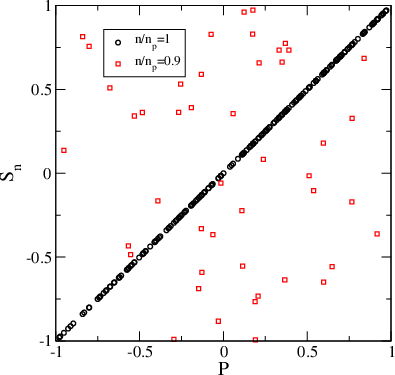
Using the eigenvectors $\psi_{p}(x)$ and eigenvalues $\lambda_{p}$ of the quark operator, the Polyakov loop $P(\boldmathe{x})$ in (2) can be reconstructed at position $\boldmathe{x}$ by

$$\begin{split}{\mathcal{S}}_{n}(x)&:=\frac{1}{8}\sum_{p=1}^{n}\left(\varrho_{p}(x)\lambda_{p}^{N_{t}}-{{}^{z}\!\varrho}_{p}(x)\,{{}^{z\!}\lambda}_{p}^{N_{t}}\right),\\ P(\boldmathe{x})&={\mathcal{S}}_{n_{p}}(x_{0},\boldmathe{x}),\quad\forall x_{0}\end{split}$$ (130)

where $n_{p}=2N_{t}N_{s}^{3}$ is the total number of eigenmodes. It was already observed earlier that the mode sum in (130) is dominated by the high end of the Dirac spectrum. Restricting the mode sum to a smaller upper limit $n\ll n_{p}$, we do not expect that $P(\boldmathe{x})$ and ${\mathcal{S}}_{n}(x)$ are correlated locally. In order to explore which value of $n$ must be used to obtain a satisfactory agreement, we chose $n=0.9\,n_{p}$ and produced the scatter plot in Figure 4, left panel. For $n=n_{p}$, we observe a perfect correlation (which served as a benchmark test for our numerical approach). Already for $n$ as high as $0.9\,n_{p}$, this correlation has disappeared. A similar result holds for the expectation value of the Polyakov loop [8, 9, 10].

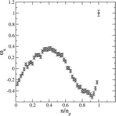
In order to quantify this correlation, we introduce

$$\omega_{n}=\frac{\Bigl\langle P(\boldmathe{x})\,{\mathcal{S}}_{n}(x_{0},\boldmathe{x})\Bigr\rangle_{x}}{\sqrt{\Bigl\langle P^{2}(\boldmathe{x})\Bigr\rangle_{x}\,\Bigl\langle{\mathcal{S}}_{n}^{2}(x_{0},\boldmathe{x})\Bigr\rangle_{x}}}.$$ (131)

The average extends over the space-time index, and only contributions from a single lattice configuration are taken into account. If $P$ and ${\mathcal{S}}_{n}$ are completely uncorrelated, we find (in the confining phase)

$$\frac{\langle P\rangle}{\sqrt{\langle P^{2}\rangle}}\approx 0,\quad\frac{\langle{\mathcal{S}}_{n}\rangle}{\sqrt{\langle{\mathcal{S}}^{2}_{n}\rangle}}\approx 0,\quad\omega_{n}\approx 0.$$ (132)

By contrast, if both quantities are perfectly correlated, i.e., $P\propto{\mathcal{S}}_{n}$, we obtain $\omega_{n}\approx 1$. Figure 4, right panel, shows $\omega_{n}$ as a function of $n/n_{p}$, which is the fraction of the spectrum which was considered for the mode sum (130). Although the correlation is perfect for $n/n_{p}\to 1$, a decent correlation is only achieved if almost all of the spectrum is taken into account.

Figure 5: The correlation measure $\omega_{n}$ (131) as a function of $n/n_{p}$ for different types of mode sums, single lattice configuration, $6^{4}$ lattice (right).

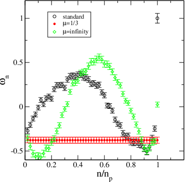
Let us complete this subsection by replacing the mode sum ${\mathcal{S}}_{n}$ in (130) by the IR weighted sum

$${\mathcal{G}}_{n}(x):=\frac{1}{8}\sum_{p=1}^{n}\left(\varrho_{p}(x)e^{-\lambda^{2}_{p}/\mu^{2}}-{{}^{z}\!\varrho}_{p}(x)e^{-{{}^{z\!}\lambda}^{2}_{p}/\mu^{2}}\right).$$ (133)

In complete analogy to (131), we may define $\omega_{n}^{\mathcal{G}}$ which quantifies the correlation between the Polyakov loop at each point in space and ${\mathcal{G}}_{n}(x_{0},\boldmathe{x})$. Figure 5 shows our findings for $\mu=1/3$ and $\mu\rightarrow\infty$ in comparison with $\omega_{n}$ in (131). The $\mu=1/3$ graph hardly shows a dependence on $n/n_{p}$ simply because the mode sum is already efficiently damped by the exponential factor. In the intermediate range $0.4<n/n_{p}<0.7$, the mode sum utilizing $\mu\rightarrow\infty$ has a sizable correlation with the Polyakov loop.

VI.4 The static potential

   

Figure 6: The static quark potential extracted from the truncated mode sum (135) and from the Polyakov loop correlator (134) in the confinement phase ($N_{t}=6$) and in deconfinement phase $(N_{t}=2)$ (left panel). The potentials for $T\approx T_{c}$, $(N_{t}=4)$ (right panel).

On the other hand, we do expect that the expectation value for the Polyakov loop correlator

$$C(r)=\Bigl\langle P(\boldmathe{x})\,P(\boldmathe{x}+r\boldmathe{e}_{3})\Bigr\rangle$$ (134)

is dominated by the IR regime of Yang-Mills theory at least for sufficiently large separations $r$. We therefore define the mode sum approximation to $C(\boldmathe{x},r)$ by

$$C^{\,{\mathcal{G}}}_{n}(r)=\Bigl\langle{\mathcal{G}}_{n}(x_{0},\boldmathe{x})\,{\mathcal{G}}_{n}(x_{0},\boldmathe{x}+r\boldmathe{e}_{3})\Bigr\rangle.$$ (135)

Note that the expectation value on the right hand side of the latter equation does not depend on the particular choice for $x_{0}$ due to translational invariance. From the above correlation functions, the static quark potential $V(r)$ and its mode sum approximation $V^{\,{\mathcal{G}}}(r)$ is obtained from

$$V(r)/T=-\ln C(r),\quad V^{\,{\mathcal{G}}}(r)/T=-\ln C^{\,{\mathcal{G}}}_{n}(r),$$ (136)

where $T$ is the temperature. In this first numerical study, we have chosen the exponential mode sum with $\mu^{2}=0.1$ and truncated the mode sum by setting $n=50$. Thus, the lowest $50$ eigenvalues contributed.

We also investigated the deconfinement phase transition which takes place if the temperature exceeds the critical value $T_{c}\approx 0.69(2)\,\sqrt{\sigma}$ [30]. Temperature is adjusted by varying the temporal extent $N_{t}$ of the $N_{t}\times N_{s}^{3}$ lattice:

$$\frac{T}{\sqrt{\sigma}}=\frac{1}{N_{t}\,\sqrt{\sigma a^{2}}}\;.$$ (137)

Our simulations parameters are summarized in Table 2.

Table 2: simulation parameters

$\beta$	$\sigma a^{2}$	lattice	$T/T_{c}$	configurations
$1.35$	$0.1244(7)$	$12^{3}6$	$0.7$	$8658$
$1.35$	$0.1244(7)$	$12^{3}4$	$1.0$	$12000$
$1.35$	$0.1244(7)$	$12^{3}2$	$2.1$	$12000$

Figure 6, left panel, shows the potentials $V^{{\mathcal{G}}}(r)$ in comparison with the full static potential $V(r)$ in the confinement phase for $N_{t}=6$. Most striking is that the potential $V^{{\mathcal{G}}}(r)$ linearly rises at large distances $r$ and therefore shows confining behavior. At small distances $r$, the potential $V^{{\mathcal{G}}}(r)$ is flat and does not show any sign of Coulomb law. This was not expected since the $1/r$ part arises from the exchange of gluons and belongs to the realm of the UV regime. The rather flat behavior implies a constant correlation at short distances and points toward a rather smooth field ${\mathcal{G}}_{n}(x)$.

Also shown in Figure 6 are both potentials, i.e., $V^{{\mathcal{G}}}(r)$ and $V(r)$, in high temperature regime. At temperatures $T\approx 2T_{c}$, both potential are essentially flat, and, in particular $V^{{\mathcal{G}}}(r)$, has lost any signal of the linear rise.

The situation is less clear for $T\approx T_{c}$ in Figure 6, right panel. While the Polyakov loop correlator can be, to a good extent, fitted by a $1/r$ Coulomb law, the mode sum still shows a significant linear rise. The interesting question is whether in the case of the mode sum the shift of the critical temperature to higher values is nonvanishing in the continuum limit. To answer this question, much more time consuming simulations using higher values of $\beta$ and therefore larger lattices are necessary. It would also be interesting to study the critical temperature signalled by $V^{{\mathcal{G}}}(r)$ for several types of mode sums. This is left to future work.

VI.5 Visualization

Figure 7: The mode sum $|{\mathcal{G}}_{n}(x)|$ in a $20^{3}$ spatial hypercube. Side length of the cube: $3.2\,$fm.

The potential $V^{{\mathcal{G}}}(r)$ flattens for small quark antiquark distances $r$. This indicates that the mode sums ${\mathcal{G}}_{n}(x)$ in (133) are rather smooth functions of $x$. In order to get a first impression of the space texture of these mode sums, in Figure 7 we have visualized

$$|{\mathcal{G}}_{n}(x)|,\quad n=25,\quad\mu=\frac{1}{3}$$

within the spatial hypercube of a particular $20^{3}\times 8$ lattice configuration. The lattice configuration was generated with the improved action [29] using $\beta=1.35$. Using $\sigma=(440\mathrm{MeV})^{2}$ and $\sqrt{\sigma a^{2}}\approx 0.124$, the length of the cube is roughly $3.2\,$fm. Thus, we observe a texture which is rather smooth at the length scale of $0.3\,$fm. This explains the behavior of the mode sum correlator (135) at short distances.

VII Conclusions

It is generally accepted that the low lying modes of the quark operator bear witness of the spontaneous breakdown of chiral symmetry in QCD. Here, we have investigated to which extent the low lying modes also contain information on quark confinement.

For this purpose, Gattringer’s mode sum approach [8] to the Polyakov loop expectation value $\sum_{x}P(\boldmathe{x})$ has been generalized to reconstruct the Polyakov loop locally. We have also pointed out that the mode sum approach is not restricted to lattice Dirac operators, but can be directly formulated in the continuum formulation of Yang-Mills theory. The existence of these sums has been studied in some detail. If one first sums over the center elements and afterwards over the eigenvalues, then the spectral sums exist for all polynomial functions of the Dirac operator, especially for the IR dominated mode sums of interest, for example for $1/{\mathcal{D}}_{A}^{2}$. We have argued that the IR dominated mode sums equally well form an order parameter for confinement since these sums and the Polyakov loop share the same center transformation property.

We have thoroughly investigated these mode sums by means of analytical calculations in the context of the Schwinger model and of $SU(2)$ gauge theory in the background of homogeneous field strength. As expected for these examples, the mode sums are proportional to the Polyakov loop for each point in space.

Subsequently, we have employed $SU(2)$ lattice gauge simulations to study the relation between the low lying modes of the Dirac operator and the static quark antiquark potential. Below the critical deconfinement temperature, the correlator between two IR dominated mode sums is able to describe a linearly rising confining potential at large distances $r$. In the high temperature deconfined phase, this correlator reflects the flat behavior of the potential at large distances, and is in very good agreement with the correlator of two Polyakov lines. This clearly shows that the quark confinement mechanism is entirely encoded in the low lying spectrum of the Dirac operator. The search for confining degrees of freedom, such as vortices or monopoles, in the IR regime of the Dirac operator is left to future work.

We finally point out that the preprint [31] appeared shortly after we made this work available electronically. In this preprint, Bilgici and Gattringer also put forward the mode sum approach to the Polyakov line correlator and provided complementary numerical insights for the gauge group SU(3).

*

Appendix A Poisson resummation for harmonic oscillator eigenfunctions

In this appendix we consider and resum the eigenfunctions of the squared Dirac operator $-{\mathcal{D}}_{A}^{2}$ for the Schwinger model on the torus. We measure Euclidean time in units of $\beta$ and lengths in units of $L$. We assume that the flux $\Phi=2\pi q$ entering the gauge potential

$$A_{0}=-\Phi x_{1}+2\pi h_{0}\quad\hbox{{and}}\quad A_{1}=2\pi h_{1}$$ (138)

is positive. The periodic eigenmodes on the cylinder $[0,1]\times\mathbb{R}$ have the form

$$\chi_{p,\ell}(x)=e^{2\pi i\ell x_{0}}e^{2\pi ih_{1}x_{1}}\xi_{p}(y^{1})$$ (139)

with $y^{1}=x_{1}+\frac{1}{q}\left(\ell-h_{0}\right),$ where $\ell\in\mathbb{Z}$ and the mode functions $\xi_{p}$ are eigenfunctions of $a^{\dagger}a$,

$$a^{\dagger}a\,\xi_{p}=2p\xi_{p},\quad a=(2\pi q)^{\frac{1}{2}}y^{1}+(2\pi q)^{-\frac{1}{2}}\partial_{y^{1}}$$ (140)

with $[a,a^{\dagger}]=2$. The dependence on $\ell$ enters via the $\ell$-dependence of $y^{1}$. The normalized modes are

$$\xi_{p}(y)=c_{p}a^{\dagger p}\xi_{0}(y)$$ (141)

with

$$c_{p}^{2}=\frac{1}{2^{p}p!}\quad\hbox{{and}}\quad\xi_{0}(x)={(2q)^{1/4}}\,e^{-\pi qx^{2}}.$$ (142)

The normalized eigenfunctions on the torus with boundary conditions (59) are superpositions of the modes on the cylinder,

$$\begin{split}\psi_{p,\ell}(x)&=\sum_{s}e^{2\pi ish_{1}}\chi_{p,\ell+sq}(x)\\ &=e^{-2\pi iqx_{0}x_{1}}e^{2\pi i(h_{0}y^{0}-\ell h_{1}/q)}\sum_{s}f_{p}(y^{1}+s),\end{split}$$ (143)

where we introduced the auxiliary function

$$f_{p}(y^{1})=e^{2\pi iqy^{0}y^{1}}\xi_{p}(y^{1})\quad\hbox{{with}}\quad y^{0}=x_{0}+\frac{h_{1}}{q}.$$ (144)

Here we can apply the Poisson resummation formula

$$\begin{split}\sum_{s}f(y^{1}+s)&=\sum_{m}e^{-2\pi imy}\tilde{f}(m),\\ \tilde{f}(\eta)&=\int_{-\infty}^{\infty}dy^{1}\,e^{2\pi i\eta y^{1}}f(y^{1}),\end{split}$$ (145)

and together with $\tilde{f}_{p}(\eta)=\tilde{\xi}_{p}(\eta+qy^{0})$ it leads to

$$\psi_{p,\ell}(x)=e^{-2\pi iqx_{0}x_{1}}e^{2\pi i(h_{0}y^{0}-\ell h_{1}/q)}\\ \times\sum_{m}e^{-2\pi imy^{1}}\,\tilde{\xi}_{p}(m+qy^{0})$$ (146)

For the $q$ ground states the corresponding sums are Gaussian and give rise to theta functions [25]. To perform the sums for the excited states we observe that under a Fourier transformation the step operators (140) are transformed into step operators,

$$\widetilde{(a^{\dagger}f)}(\eta)=i\tilde{a}^{\dagger}\tilde{f}(\eta),$$ (147)

where

$$\tilde{a}^{\dagger}=(2\pi\tilde{q})^{\frac{1}{2}}\eta-(2\pi\tilde{q})^{-\frac{1}{2}}\partial_{\eta}$$ (148)

with dual ’instanton number’ $\tilde{q}$ related to $q$ by

$$q\tilde{q}=1.$$ (149)

The step operators $\tilde{a},\tilde{a}^{\dagger}$ obey the same commutation relations as $a,a^{\dagger}$. Since the ground state $\xi_{0}$ is transformed into the ground state with $\tilde{q}$ we conclude that

$$\tilde{\xi}_{p}(\eta)=c_{p}\widetilde{(a^{\dagger p}\xi_{0})}=i^{p}c_{p}\tilde{a}^{\dagger p}\tilde{\xi}_{0}$$ (150)

with $\tilde{\xi}_{0}(\eta)={(2\tilde{q})^{1/4}}\,e^{-\pi\tilde{q}\,\eta^{2}}$. In calculations it is advantageous to use Hermite polynomials $H_{p}$ generated by $a^{\dagger}$ and $\tilde{a}^{\dagger}$

$$\begin{split}a^{\dagger p}\xi_{0}(y)&=H_{p}\left(\sqrt{2\pi q}\cdot y\right)\xi_{0}(y),\\ \tilde{a}^{\dagger p}\tilde{\xi}_{0}(\eta)&=H_{p}\left(\sqrt{2\pi\tilde{q}}\cdot\eta\right)\tilde{\xi}_{0}(\eta).\end{split}$$ (151)

In terms of these polynomials the equivalent series (143) take the form

$$\psi_{p,\ell}(x)=c_{p}\,e^{2\pi i\ell x_{0}}e^{2\pi ih_{1}x_{1}}\\ \times\sum_{m}e^{2m\pi iqy^{0}}H_{p}\left(\sqrt{2\pi q}\,(y^{1}+m)\right)\xi_{0}(y^{1}+m)$$ (152)

and the resummed series (146) reads

$$\psi_{p,\ell}(x)=\frac{i^{p}c_{p}}{\sqrt{q}}\,e^{-2\pi iqx_{0}x_{1}}e^{2\pi i(h_{0}y^{0}-\ell h_{1}/q)}\\ \times\sum_{m}e^{-2m\pi iy^{1}}H_{p}\left(\sqrt{2\pi q}\,\big(y^{0}+\frac{m}{q}\big)\right)\xi_{0}\big(y^{0}+\frac{m}{q}\big).$$ (153)

In the main body of the paper we used antiperiodic eigenmodes of the Dirac operator. These are obtained by replacing $h_{0}\to h_{0}+1/2$ and $\ell\to\ell-1/2$ in the results (152) and (153).

References

- [1] Frithjof Karsch. Deconfinement and chiral symmetry restoration. arXiv:hep-lat/9903031.
- [2] Frithjof Karsch and Martin Lutgemeier. Deconfinement and chiral symmetry restoration in an SU(3) gauge theory with adjoint fermions. Nucl. Phys., B550:449–464, 1999.
- [3] L. Del Debbio, M. Faber, J. Greensite, and S. Olejnik. Center dominance and Z(2) vortices in SU(2) lattice gauge theory. Phys. Rev., D55:2298–2306, 1997.
- [4] Kurt Langfeld, Hugo Reinhardt, and Oliver Tennert. Confinement and scaling of the vortex vacuum of SU(2) lattice gauge theory. Phys. Lett., B419:317–321, 1998.
- [5] J. Greensite. The confinement problem in lattice gauge theory. Prog. Part. Nucl. Phys., 51:1, 2003.
- [6] M. Engelhardt, K. Langfeld, H. Reinhardt, and O. Tennert. Deconfinement in SU(2) Yang-Mills theory as a center vortex percolation transition. Phys. Rev., D61:054504, 2000.
- [7] Jochen Gattnar et al. Center vortices and Dirac eigenmodes in SU(2) lattice gauge theory. Nucl. Phys., B716:105–127, 2005.
- [8] Christof Gattringer. Linking confinement to spectral properties of the Dirac operator. Phys. Rev. Lett., 97:032003, 2006.
- [9] Falk Bruckmann, Christof Gattringer, and Christian Hagen. Complete spectra of the Dirac operator and their relation to confinement. Phys. Lett., B647:56–61, 2007.
- [10] Franziska Synatschke, Andreas Wipf, and Christian Wozar. Spectral sums of the Dirac-Wilson operator and their relation to the Polyakov loop. Phys. Rev., D75:114003, 2007.
- [11] Wolfgang Soldner. The Polyakov Loop and the Eigenvalues of the Dirac Operator. PoS, LAT2007:222, 2007.
- [12] Christian Hagen, Falk Bruckmann, Erek Bilgici, and Christof Gattringer. Thin and dressed Polyakov loops from spectral sums of lattice differential operators. arXiv:0710.0294 [hep-lat]
- [13] Erek Bilgici, Falk Bruckmann, Christof Gattringer, and Christian Hagen. Dual quark condensate and dressed Polyakov loops. arXiv:0801.4051 [hep-lat]
- [14] Falk Bruckmann, Stefan Keppeler, Marco Panero, and Tilo Wettig. Polyakov loops and SU(2) staggered Dirac spectra. arXiv:0802.0662 [hep-lat]
- [15] F. Bruckmann and E. M. Ilgenfritz. Laplacian modes probing gauge fields. Phys. Rev., D72:114502, 2005.
- [16] Pierre van Baal. Some Results for SU(N) Gauge Fields on the Hypertorus. Commun. Math. Phys., 85:529, 1982.
- [17] C. Ford, U. G. Mitreuter, T. Tok, A. Wipf, and J. M. Pawlowski. Monopoles, Polyakov loops, and gauge fixing on the torus. Annals Phys., 269:26–50, 1998.
- [18] H. Weyl. Das asymptotische Verteilungsgesetz der Eigenwerte linearer partieller Differentialgleichungen (mit einer Anwendung auf die Theorie der Hohlraumstrahlung). Math. Ann., 71:441–479, 1912.
- [19] W. Nahm. A Simple Formalism for the BPS Monopole. Phys. Lett., B90:413, 1980.
- [20] Gerard ’t Hooft. Topology of the Gauge Condition and New Confinement Phases in Nonabelian Gauge Theories. Nucl. Phys., B190:455, 1981.
- [21] S. Minakshisundaram and A. Pleijel. Some properties of the eigenfunctions of the Laplace-operator on Riemannian manifolds. Can. J. Math., 1:242, 1949.
- [22] Peter B. Gilkey. Invariance Theory, the Heat Equation, and the Atiyah-Singer Index Theorem. Publish or Perish Inc., USA, 1984.
- [23] Albert S. Schwarz. Instantons and fermions in the field of instanton. Commun. Math. Phys., 64:233–268, 1979.
- [24] Steve Blau, Matt Visser, and Andreas Wipf. Determinants, Dirac operators, and one loop physics. Int. J. Mod. Phys., A4:1467, 1989.
- [25] I. Sachs and A. Wipf. Finite temperature Schwinger model. Helv. Phys. Acta, 65:652–678, 1992.
- [26] I. S. Gradshteyn and I. M. Ryzhik. Table of Integrals, Series, and Products. Academic Press, corrected and enlarged edition, 1980.
- [27] Arthur Erdélyi, Wilhelm Magnus, Fritz Oberhettinger, and Francesco Tricomi. Higher Transcendental Functions, Volume II. McGraw-Hill Book Company, 1953.
- [28] R. L. Hall, N. Saad, and A. B. von Keviczky. Closed-form sums for some perturbation series involving associated Laguerre polynomials. Journal of Physics A: Mathematical and General, 34(50):11287–11300, 2001.
- [29] Kurt Langfeld. Improved actions and asymptotic scaling in lattice Yang- Mills theory. Phys. Rev., D76:094502, 2007.
- [30] J. Fingberg, Urs M. Heller, and F. Karsch. Scaling and asymptotic scaling in the SU(2) gauge theory. Nucl. Phys., B392:493–517, 1993.
- [31] E. Bilgici and C. Gattringer, Static quark-antiquark potential and Dirac eigenvector correlators. arXiv:0803.1127 [hep-lat].