MATRIX GRAPH GRAMMARS

by

Pedro Pablo Pérez Velasco

Version 1.2

© Copyright by
Pedro Pablo Pérez Velasco
2007, 2008, 2009

To my family

ACKNOWLEDGEMENTS

These lines are particularly pleasant to write. After all those years, I have a quite long list of people that have contributed to this book in one way or another. Unfortunately, I will not be able to include them all. Apologizes for the absences.

First of all my family. Gema, with neverending patience and love, always supports me in every single project that I undertake. My unbounded love and gratitude. Hard to return, though I’ll try. My two daughters, Sofía and Diana, make every single moment worthy. I’m absolutely grateful for their existence.

My brothers Álex and Nina, now living in Switzerland, with whom I shared so many moments and that I miss so much. My parents, always supporting also with patience and love, worried if this boy would become a man (am I?).

Juan, my thesis supervisor, whose advice and interest is invaluable. He has been actively involved in this project despite his many responsibilities. Also, I would like to thank the people at the series of seminars on complexity theory at U.A.M., headed by Roberto Moriyón, for their interest on Matrix Graph Grammars.

Many friends have stoically stood some chats on this topic affecting interest. Thank you very much for your friendship. KikeSim, GinHz, Álvaro Iglesias, Jaime Guerrero, … All those who have passed by are not forgotten: People at ELCO (David, Fabrizio, Juanjo, Julián, Lola, …), at EADS/SIC (Javier, Sergio, Roberto, …), at Isban, at Banco Santander. Almost uncountable.

I am also grateful to those that have worked on the tools used in this book: Emacs and microEmacs, MikTeX, TeTeX, TeXnicCenter, OpenOffice and Ubuntu. I would like to highlight the very good surveys available on different topics on mathematics at the web, in particular at websites http://mathworld.wolfram.com and http://en.wikipedia.org, and the anonymous people behind them.

Last few years have been particularly intense. A mixture of hard work and very good luck. I feel that I have received much more than I’m giving. In humble return, I will try to administer http://www.mat2gra.info, with freely available information on Matrix Graph Grammars such as articles, seminars, presentations, posters, one e-book (this one you are about to read) and whatever you may want to contribute with.

Chapter Introduction

This book is one of the subproducts of my dissertation. If its aim had to be summarized in a single sentence, it could be algebraization of graph grammars or, more accurately, study of graph dynamics.

From the point of view of a computer scientist, graph grammars are a natural generalization of Chomsky grammars for which a purely algebraic approach does not exist up to now. A Chomsky (or string) grammar is, roughly speaking, a precise description of a formal language (which in essence is a set of strings). On a more discrete mathematical style, it can be said that graph grammars – Matrix Graph Grammars in particular – study dynamics of graphs. Ideally, this algebraization would enforce our understanding of grammars in general, providing new analysis techniques and generalizations of concepts, problems and results known so far.

In this book we fully develop such theory over the field $GF(2)$ – the field with two elements – which covers all graph cases, from simple graphs (more attractive for a mathematician) to multidigraphs (more interesting for an applied computer scientist). The theory is presented and its basic properties demonstrated in a first stage, moving to increasingly difficult problems and establishing relations among them:

• Applicability, for which two equivalent characterizations (necessary and sufficient conditions) are provided.

• Independence. Sequential and parallel independence in particular, generalizing previously known results for two elements.

• Restrictions. The theory developed so far for graph constraints and application conditions is significantly generalized.

• Reachability. The state equation for Petri nets and related techniques are extended to general Matrix Graph Grammars. Also, Matrix Graph Grammars techniques are applied to Petri nets.

Throughout the book many new concepts are introduced such as compatibility, coherence, initial and negative graph sets, etc. Some of them project interesting insights about a given grammar, while others are used to study previously mentioned problems.

Matrix Graph Grammars have several advantages. First, many branches of mathematics are at our disposal. It is based on Boolean algebra, so first and second order logics can be applied almost directly. They admit a functional representation so many ideas from functional analysis can be utilized. On the more algebraic side it is possible to use group theory and tensor algebra. Finally, category theory constructions such as pushouts are available as well. Second, as it splits the static definition from the dynamics of the system, it is possible to study to some extent many properties of the grammar without the need of an initial state. Third, although it is a theoretical tool, Matrix Graph Grammars are quite close to implementation, being possible to develop tools based on this theory.

This introductory chapter aims to provide some perspective on graph grammars in general and on Matrix Graph Grammars in particular. In Sec. 1 we present a (partial) historical overview of graph grammars and graph transformation systems taken from several sources but mainly from [36] and [22]. Section 2 introduces those open problems that have guided our research. Finally, in Sec. 3 we brush over the book and see how applicability, sequential independence and reachability articulate it.

1 Historical Overview

Research in graph grammars started in the late 60’s [69][72], strongly motivated by practical problems in computer science and since then it has become a very active area. Currently there is a wide range of applications in different branches of computer science such as formal language theory, software engineering, pattern recognition and generation, implementation of term rewriting, logical and functional programming, compiler construction, database design and theory, visual programming and modeling languages and many more (see [23] for references on these and other topics).

There are different approaches to graph grammars and graph transformation systems. Among them, the most prominent are the algebraic, logical, relational and set-theoretical.

Figure 1: Main Steps in a Grammar Rule Application

The main steps – some of which are summarized in Fig. 1 – in all approaches for the application of a grammar rule $p:L\rightarrow R$ to a host graph $G$ (also known as initial state) to eventually obtain a final state $H$ are almost the same:

1. Select the grammar rule to be applied ($p:L\rightarrow R$ in this case). In general this step is non-deterministic.

2. Find an occurrence of $L$ in $G$. In general this step is also non-deterministic because there may be several occurrences of $L$ in $G$.

3. Check any application condition of the production.

4. Remove elements that appear in $L$ but not in $R$. There are two possibilities for so-called dangling edges:

   1. Production is not applied.

   2. Dangling edges are deleted too.

   If the production is to be applied, the system state changes from $G$ to $G_{1}$ (see Fig. 1).

5. Glue $R$ with $G_{1}$. The system state changes from $G_{1}$ to $H$ (see Fig. 1).

Now we shall briefly review previously mentioned families of approaches. The so-called algebraic approach to graph grammars (graph transformation systems) is characterized by relying almost exclusively on category theory and using gluing of graphs to perform operations. It can be divided into at least three main sub approaches, depending on the categorical construction under use: DPO (Double PushOut, see Sec. 11), SPO (Single PushOut, see Sec. 12), pullback and double pullback (also summarized in Sec.  12). We will not comment on others, like sesquipushout for example (see [9]).

DPO was initiated by Ehrig, Pfender and Schneider in the early 70’s [21] as a generalization of Chomsky grammars in order to consider graphs instead of strings. It seems that the term algebraic was appended because graphs might be considered as a special kind of algebras and because the pushout construction was perceived more as a concept from universal algebra than from category theory. Nowadays it is the more prominent approach to graph rewriting, with a vast body of theoretical results and several tools for their implementation.

By mid and late 80’s Raoult [70], Kennaway [41][42] and Löwe [49] developed SPO approach probably motivated by some “restrictions” of DPO, e.g. the usage of total instead of partial morphisms. Raoult and Kennaway were focused on term graph rewriting while Löwe took a more general approach.

In the late 90’s a new approach – although less prominent for now – emerged by reverting all arrows (using pullbacks instead of pushouts), proposed by Bauderon [5]. It seems that, in contrast to the pushout construction, pullbacks can handle deletion and duplication more easily.

DPO has been generalized recently through adhesive HLR categories, which is summarized in Sec. 12 (we are not aware of a similar initiative for SPO or pullback). For a detailed account see [22]. Instead of just considering graphs, all main ideas in DPO can be extended to higher level structures like labeled graphs, typed graphs, Petri nets, etc. This is firstly accomplished in [16] and [17], starting the theory of HLR systems (High Level Replacement systems). Independently, Lack and Sobociński in [43] introduced the concept of adhesive category and in [18] both were merged to get adhesive HLR categories.

In this book we shall refer to these approaches as categorical, to distinguish from ours which is more algebraic in nature.

The so-called set-theoretic approach (sometimes also known as algorithmic approach) substitutes one structure by another structure, either nodes or edges. There are two subfamilies, node replacement and edge replacement (also hyperedge replacement), depending on the type of elements to be replaced. Node replacement (edNCE) was introduced in [55][56] and further investigated in many papers. It is based on connecting instead of gluing for embedding one graph into another. Many extensions and particular cases have been studied so far, and many others, such as C-edNCE when considering confluence, NCE, NLC, dNLC, edNLC and edNCE (see Sec. 13 for the meaning of acronyms) are currently on going. Hyperedge replacement was introduced in the early 70s by Feder [27] and Pavlidis [59] and has been intensively investigated since then. Contrary to the node replacement approach, it is based on gluing. Please, see Secs. 13 and 14 for a quick introduction.

It is possible to use logics to express graphs and to encode graph transformation. In Sec. 15 this approach with monadic second order logic is reviewed presenting its foundations and main results.

The relational approach (also algebraic-relational approach) is based on relational methods to specifying graph rewriting (in fact it could be applied to more general structures than graphs). Once a graph is characterized as a relational structure it is possible to apply all relational machinery, substituting categories by allegories and Dedekind categories. Probably, the main advantage is that it is possible to give local characterization of concepts. The roots of this approach seem to date back to the early 1970’s with the papers of Kawahara [38][39][40] establishing a relational calculus inside topos theory. An overview can be found in Sec. 16.

Our approach has been influenced by these approaches to a different extent, heavily depending on the topic. The basics of Matrix Graph Grammars are most influenced by the categorical approach, mainly by SPO in the shape of productions and to some extent of direct derivations. For application conditions and graph constraints, our inspiration comes almost exclusively from MSOL. Concerning the relational approach, our basic structure has a natural representation in relational terms but the development in both cases is very different. The influence of hyperedge replacement and node replacement, if any, is much more fuzzy.

2 Motivation

The dissertation that gave rise to this book started as a project to study simulation protocols (conservative, optimistic, etc.) under graph transformation systems. In the first few weeks we missed a real algebraic approach to graph grammars. “Real” in the sense that there are algebraic representations of graphs very close to basic algebraic structures such as vector spaces (incidence or adjacency matrices for example) but the theories available so far do not make use of them. As commented above, the main objective of this book is to give an algebraization of graph grammars.

One advantage foreseen from the very beginning was the fact that nice interpretations in terms of functional analysis and physics could be used to move forward, despite the fact that the underlying structure is binary so, if necessary, it was possible to bring in easily logics and its powerful methods.

Our schedule included several increasingly difficult problems to be treated by our approach with the hope of getting better insight and understanding, trying to generalize whenever possible and, most importantly, providing a unified body of results in which all concepts and ideas would fit naturally.

First things first, so we begin with the name of the book: Matrix Graph Grammars. It has been chosen to emphasize the algebraic part of the approach -- although there are also logics, tensors, operators -- and to recall matrix mechanics as introduced by Born, Heisenberg and Jordan in the first half of the twentieth century. You are kindly invited to visit http://www.mat2gra.info for further research, a web page dedicated to this topic that I (hopefully) intend to maintain.

Section 1 points out that motivations of some graph grammar approaches have been quite close to practice, in contrast with Matrix Graph Grammars (MGG) which is more theoretically driven. Nonetheless, there is an on-going project to implement a graph grammar tool based on $\textrm{AToM}^{3}$ (see [45] or visit http://atom3.cs.mcgill.ca/) using algorithms derived from this book (the analysis algorithms are expected to have a good performance). We will briefly touch on this topic in Sec. 29. Appendix id1 illustrates all the theory with a more or less realistic case study.

This “basis for theoretical studies” intends to provide us with the capability of solving theoretical problems as those commented below, which are the backbone of the book.

Informally, a grammar is a set of productions plus an initial graph which we can safely think of as a collection of functions plus an initial set. A sequence of productions would then be a sequence of functions, applied in order. Together with the function we specify the elements that must be found in the initial set (in its domain), so in order to apply a function we must first find the domain of the function in the initial set (this process is known as matching). As productions are applied, the system moves on transforming the initial set in a sequence of intermediate sets to eventually arrive to a final state (final set). Actually, we will deal neither with sets nor with functions but with directed graphs and morphisms.

We will speak of graphs, digraphs or simple digraphs meaning in all cases simple digraphs. See Sec. 6 for its definition and main properties.

Once grammar rules have been defined and its main properties established, the first problem we will address is the characterization of applicability, i.e. give necessary and sufficient conditions to guarantee that a sequence can be applied to an initial state (also known as host graph) to output a final state (a graph again). Formally stated for further reference:

Problem 1 (Applicability)

For a sequence $s_{n}$ made up of rules in a grammar $\mathfrak{G}$ and a simple digraph $G$, is it possible to apply $s_{n}$ to the host graph $G$?

No restriction is set on the output of the sequence except that it is a simple digraph. There is a basic problem when deleting nodes known as dangling condition: Are all incident edges eliminated too? Otherwise the output would not be a digraph.

When we have a production and a matching (for that production) we will speak of a direct derivation. A sequence of direct derivations is called a derivation.

A quite natural progression in the study of grammars is the following question, that we call independence problem:

Problem 2 (Independence)

For two given derivations $d_{n}$ and $d^{\prime}_{n}$ applicable to host graph $G$, do they reach the same state?, i.e. is $d_{n}(G)=d^{\prime}_{n}(G)$?

Mind the similarities with confluence and local confluence (see below). However, independence is a very general problem and we will be interested in a reduced version of it, known as sequential independence, which is widely addressed in the graph grammar literature and also in other branches of computer science. As far as we know, in the literature [23, 22] this problem is addressed for sequences of two direct derivations, being longer sequences studied pairwise.

Problem 3 (Sequential Independence)

For two derivations $d_{n}$ and $d^{\prime}_{n}=\sigma(d_{n})$ applicable to host graph $G$, with $\sigma$ a permutation, do they reach the same state?

Of course, problems 2 and 3 can be extended easily to consider any finite number of derivations and, in both cases, there is a dependence relationship with respect to problem 1.

Our next step will be to generalize some theory from Petri nets [54], which can be seen as a particular case of Matrix Graph Grammars. In particular, our interest is focused on reachability:

Problem 4 (Reachability)

For two given states (initial $S_{0}$ and final $S_{T}$), is there any sequence made up of productions in $G$ that transforms $S_{0}$ into $S_{T}$?

In the theory developed so far for Petri nets, reachability is addressed using the state equation (linear system) which is a necessary condition for the existence of such a sequence (see Chap. id1).

Problem 4 directly relies on problem 1. More interestingly, it is also related to problems 2 and 3: As every solution provided by the state equation specifies the set of productions to be applied but not the order (see Sec. 45), sequences associated to different solutions of the state equation can be independent but not sequential independent (this is because different sets of solutions apply each production a different number of times). So, in particular, reachability can be useful to split independence and sequential independence.

Figure 2: Partial Diagram of Problem Dependencies

All these problems with their corresponding dependencies are summarized in Fig. 2. Compare with the complete diagram that includes mid-term and long-term research in Fig. 120 on p. 120.

Although we will not study confluence in this book (except some ideas in Chap. id1), just to make a complete account two further related problems are introduced. We will briefly review them in the last chapter.

Problem 5 (Confluence)

For two given states $S_{1}$ and $S_{2}$, do there exist two derivations $d_{1}$ and $d_{2}$ such that $d_{1}(S_{1})\cong d_{2}(S_{2})$?.

Strictly speaking this is not confluence as defined in the literature [77]. To the left of Fig. 3 you can find confluence: For the initial state $S_{0}$ that independently evolves to $S_{1}$ and $S_{2}$, is it possible to find derivations that close the diamond? To the right of the same figure we have represented problem 5. The difference is that a common initial state is not assumed.

Figure 3: Confluence

In mathematics, existence and uniqueness theorems are central to any of its branches. As it is, the analogous terms in computer science are termination and confluence, respectively.

In some sense we may think of reachability as opening or broadening the state space of a given grammar while confluence, as introduced here, closes or bounds it.

Problem 5 deals with confluency of confluence. The other part (how to actually get to the states $S_{1}$ and $S_{2}$) is more related to reachability. Note that if one of the derivations is the identity then problem 5 becomes problem 4 (reachability).

If we limit to permutation of sequences, as in the derivation of problem 3 out of problem 2, we can pose:

Problem 6 (Sequential Confluence)

For two given initial states, do there exist two derivations (one permutation of the other) with isomorphic final states?.

Again, it is not difficult to make them consider any finite set of derivations instead of just two. Once we know if a grammar is confluent, the next step is to know how much it takes to get to its final state. This is very close to complexity. Complexity theory is not addressed in this book.

To the best of our knowledge, applicability (problem 1) has not been addressed up to now. Independence and sequential independence (problems 2 and 3) are very popular. See for example Chaps. 3 and 4 in [23]. Reachability is a key concept and has been studied and partially characterized in many papers, mainly in Petri nets theory. See [54]. Confluence is a concept of fundamental importance to grammar theory. For term rewriting systems see [30].

3 Book Outline

Based on the problems commented in previous section, the book is organized in nine chapters plus one appendix. The First three chapters, including this one, are introductory. Chapter id1 provides a short overview of needed mathematical machinery which includes some basic results from logics (first and monadic second order), category theory, tensor algebra, graph theory, functional analysis (notation and some basic results) and group theory. We have not used advanced results on any of these disciplines so probably a quick review should suffice, mainly for fixing notation.

Graph grammars approaches are discussed in Chap. id1, which essentially expands the overview in Sec. 1. Sections 11 and 12 cover algebraic approaches, for which we prefer the term categorical, as commented above. Set-theoretic approaches (node and hyperedge replacement) are covered in Secs. 13 and 14. Term rewriting through monadic second order logics is the MSOL approach, to which Sec. 15 is devoted. The chapter ends with the relational approach in Sec. 16. The objective of this chapter is to get an idea of each approach (and not to provide a detailed study) in order to, among other things, ease comparison with Matrix Graph Grammars.

Chapter id1 introduces the basics of our proposal (Sec. 18) and prepares to attack problem 1 by introducing concepts such as completion (Sec. 19), coherence, sequences (Sec. 20) and the nihilation matrix (Sec. 21).

Standing on Chapter id1, Chapter id1 studies minimal and negative initial digraphs (Secs. 23 and 24), subsequently generalized to initial digraph set in Sec. 29), composition and compatibility (Sec. 25) and theorems related to their properties and characterizations.

Chapter id1 covers an essential part of production applicability: Matching the left hand side (LHS) of a production inside the host graph. Dangling edges are covered, dealing with them with what we call $\varepsilon$-productions in Sec. 27 and further studied and classified in Sec. 30. We deal with marking in Sec. 28, which can help in case it is necessary to guarantee that several productions have to be applied in the same place. Minimal and negative initial digraphs are generalized to the initial digraph set in Sec. 29. In Sec. 31 we give two characterizations for applicability (problem 1).

We will cope with sequential independence (problem 3) for quite general families of permutations in Chap. id1. Sameness of minimal initial digraph (called $G$-congruence) for two sequences is addressed in Sec. 33; the case of two derivations is seen in Sec. 34. Explicit parallelism is studied in Sec. 35 through composition and $G$-congruence, which is related to initial digraph sets.

In Chap. id1 graph constraints and application conditions (preconditions and postconditions) are studied for Matrix Graph Grammars. They are introduced in Sec. 37 where a short overview of related concepts in other graph grammars approaches is carried out. The notion of direct derivation is extended to cope with application conditions in Matrix Graph Grammars in a very natural manner in Sec. 38 and functionally represented in Sec. 39, where they are sequentialized.

Chapter id1 continues with graph constraints and application conditions. First, some properties such as consistency are defined and characterized (Sec. 41). In Sec. 42 we show how it is possible to transform postconditions into preconditions and vice versa. Both of theoretical and of practical importance is the use of variable nodes because, among other things, it allows us to automatically extend the theory to include multidigraphs without any change of the theory of Matrix Graph Grammars in Sec. 43.

In Chap. id1 problem 4 (reachability) is tackled, extending results from Petri nets to more general grammars. Section 45 quickly introduces this theory and summarizes some basic results. Section 46 applies some Matrix Graph Grammars results from previous chapters to Petri nets. The rest of the chapter is devoted to extending Petri nets results for reachability to Matrix Graph Grammars, in particular Sec. 47 covers graph grammars without dangling edges while Sec. 48 deals with the general case.

The book ends in Chap. id1 with the conclusions and further research. A summary of what we think are our most important contributions can be found there.

Finally, in Appendix A a fully worked case study is presented in which all main theorems are applied together with detailed explanations and implementation remarks and advices.

Most of the material presented in this book has been published [60], [61], [62], [63], [64] and [65] and presented in international congresses: ICM’2006 (International Congress of Mathematicians, awarded with the second prize of the poster competition in Section 15, Mathematical Aspects of Computer Science), ICGT’2006 (International Conference on Graph Transformations), PNGT’2006 (Petri Nets and Graph Transformations), PROLE’2007 (VII Jornadas sobre Programación y Lenguajes) and GT-VC’2007 (Graph Transformation for Verification and Concurrency, in CONCUR’2007).

Some further research is now available in http://www.mat2gra.info and in the arXiv (http://arxiv.org, just look for “Matrix Graph Grammars” in their search engine). Besides, a slight generalization using Boolean complexes have appeared in [66].

Chapter Background and Theory

The Matrix Graph Grammar approach uses many mathematical theories which might seem distant one from the others. Nevertheless, there are some interesting ideas connecting them which we seize to contribute whenever possible. Matrix Graph Grammars do not depend on any novel theorem that opens a new field of research, but aims to put “old” problems in a new perspective.

There are excellent books available covering every subject of this topic. There are also excellent resources on the web. We think that this fast introduction should suffice. It is intended as a reference chapter. All concepts are highlighted in bold to ease their location.

4 Logics

Logics are of fundamental importance to Matrix Graph Grammars for two reasons. First, graphs are represented by their adjacency matrices. As we will be most concerned with simple digraphs, they can be represented by Boolean matrices (we will come back to this in Sec. 6). Second, Chap. id1 generalizes graph constraints and application conditions using monadic second order logics. Good references on mathematical logics are [48] and [74].

First-order predicate calculus (more briefly, first order logic, FOL) generalizes propositional logic, which deals with propositions: A statement that is either true or false.

FOL formulas are constructed from individual constants ($a$, $b$, $c$, etc., typically lower-case letters from the beginning of the alphabet), individual variables (x, y, z, etc., typically lower-case letters from the end of the alphabet), predicate symbols (P, Q, R, etc., typically upper-case letters), function symbols (f, g, h, etc., typically lower-case letters from the middle of the alphabet), propositional connectives ($\neg$, $\wedge$, $\vee$, $\Rightarrow$, $\Leftrightarrow$) and quantifiers ($\forall$, $\exists$). Set $\mathcal{C}$ will be that of individual constants, set $\mathcal{F}$ will be function symbols and set $\mathcal{P}$ will contain predicate symbols. Besides these elements, punctuation symbols are permitted such as parenthesis and commas.

A formula in which every variable is quantified is a closed formula (open formula otherwise). A term (formula) that contains no variable is called ground term (ground formula). The arity of any predicate function $f$ is its number of arguments, normally written as an upper index, $f^{n}$, if needed.

The rules for constructing terms and formulas are recursive: Every element in $\mathcal{C}$ is a term, as it is any individual variable and also $f^{n}(t_{1},\ldots,t_{n})$, where $f^{n}\in\mathcal{F}$ and $t_{i}$ are terms. Also, $P\in\mathcal{P}$ is a formula and the application of any propositional connective or quantifier (or both) to two or more predicates is also a formula.

In fact, constants are formulas of arity zero so it would be convenient to omit them and allow formulas of any arity. Nevertheless we will follow the traditional exposition and use the term function when arity is at least 1.

Example.$\square$As an example of FOL formula, one of the inference rules of predicate calculus is written:

$$\exists xP(x)\wedge\forall xQ(x)\Rightarrow\exists x\left[P(x)\wedge Q(x)\right].$$

It reads as if there exists $x$ for which $P$ and for all $x$ $Q$, then there exists $x$ for which $P$ and $Q$. For another example, let’s consider the language of ordered Abelian groups. It has one constant $0$, one unary function $-$, one binary function $+$ and one binary relation $\leq$.

• $0$, $x$, $y$ are atomic terms.

• $+(x,y)$, $+(x,+(y,-(z)))$ are terms, usually written in infix notation as $x+y$, $x+(y+(-z))$.

• $=(+(x,y),0)$, $\leq(+(x,+(y,-(z))),+(x,y))$ are atomic formulas, usually written in infix notation as $x+y=0$, $x+y-z\leq x+y$.

• $\left(\forall x\exists y\leq(+(x,y),z)\right)\wedge\left(\exists x=(+(x,y),0)\right)$ is a formula, more readable if written as $\left(\forall x\exists y\;x+y\leq z\right)\wedge\left(\exists x\;x+y=0\right)$. $\blacksquare$

The semantics of our language depend on the domain of discourse ($D$) and on the interpretation function $I$. The domain of discourse (also known as universe of discourse) is the set of objects we use the FOL to talk about and must be fixed in advance. In the example above, for a fixed Abelian group, the domain of discourse are the elements of the group.

For a given domain of discourse $D$ it is necessary to define an interpretation function $I$ which assigns meanings to the non-logical vocabulary, i.e. maps symbols in our language onto the domain:

• Constants are mapped onto objects in the domain.

• 0-ary predicates are mapped onto true or false, i.e. whether they are true or false in this interpretation.

• N-ary predicates are mapped onto sets of n-ary ordered tuples of elements of the domain, i.e. those tuples of members for which the predicate holds (for example, a 1-ary predicate is mapped onto a subset of $D$).

The interpretation of a formula $f$ in our language is then given by this morphism $I$ together with an assignment of values to any free variables in $f$. If $S$ is a variable assignment on $I$ then we can write $(I,S)\models f$ to mean that $I$ satisfies $f$ under the assignment $S$ ($f$ is true under interpretation $I$ and assignment $S$). Our interpretation function assigns denotations to constants in the language, while $S$ assigns denotations to free variables.

First-order predicate logic allows variables to range over atomic symbols in the domain but it does not allow variables to be bound to predicate symbols, however. A second order logic (such as second order predicate logic, [48]) does allow this, and sentences such as $\forall P[P(2)]$ (all predicates apply to number 2) can be written.

Example.$\square$Starting out with formula:

$$\beta(X)=\forall x,y,z\left[\left(P(x,y)\wedge P(x,z)\Rightarrow y=z\right)\wedge\left(P(x,z)\wedge P(y,z)\Rightarrow x=y\right)\right]$$

which expresses injectiveness of a binary relation $P$ on its domain, it is possible to give a characterization of bijection ($X$) between two sets ($Y_{1}$, $Y_{2}$):

$$\exists X\left[\beta(X)\wedge\forall x\left(Y_{1}(x)\Leftrightarrow\exists yX(x,y)\right)\wedge\left(Y_{2}(x)\Leftrightarrow\exists yX(y,x)\right)\right].$$

The bijection $X$ is a binary relation and the sets $Y_{1}$ and $Y_{2}$ are unary relations. Hence, $Y_{1}(x)$ is the same as $x\in Y_{1}$. See [23], pp. 319-320 for more details.

Another example is the least upper bound (lub) property for sets of real numbers (every bounded, nonempty set of real numbers has a supremum):

$$\forall A\left[\left(\exists w(w\in A)\wedge\exists z\forall w(w\in A\Rightarrow w\leq z)\right)\Rightarrow\exists x\forall y\left(\forall w\in A,(w\leq y)\Leftrightarrow x\leq y\right)\right].$$

$\blacksquare$

Second order logic (SOL) is more expressive than FOL under standard semantics: Quantifiers range over all sets or functions of the appropriate sort (thus, once the domain of the first order variables is established, the meaning of the remaining quantifiers is fixed). It is still possible to increase the order of the logic, for example by allowing predicates to accept arguments which are themselves predicates.

Chapter id1 makes use of monadic second order logic, MSOL for short, which lies in between first order and second order logics. Instead of allowing quantification over n-ary predicates, MSOL quantifies 0-ary and 1-ary predicates, i.e. individuals and subsets. There is no restriction on the arity of predicates.

A theorem by Büchi and Elgot [7][26] (see also [78]) states that string languages generated by MSOL formulas correspond to regular languages (see also Sec. 15), so we have an alternative to the use of regular expressions, appropriate to express patterns (this is one of the reasons to make use of them in Chap. id1). Another reason is that properties as general as 3-colorability of a graph (see [23], Chap. 5 and also Sec. 37) can be encoded using MSOL so, for many purposes, it seems to be expressive enough.

5 Category Theory

Category theory was first introduced by S. Eilenberg and S. Mac Lane in the early 1940s in connection with their studies in homology theory (algebraic topology). See [25]. The reference book in category theory is [50]. There are also several very good surveys on this topic on the web such as http://www.cs.utwente.nl/~fokkinga/mmf92b.pdf.

A category $\mathcal{C}$ is made up of a class of objects, a class of morphisms and a binary operation called composition of morphisms, $\left(Obj(\mathcal{C}),Hom(\mathcal{C}),\circ\right)$. Each morphism $f$ has a unique source object and a unique target object, $f:A\rightarrow B$. There are two axioms for categories:

1. if $f:A\rightarrow B$, $g:B\rightarrow C$ and $h:C\rightarrow D$ then $h\circ(g\circ f)=(h\circ g)\circ f$ (associativity).

2. $\forall X\;\exists 1_{X}:X\rightarrow X$ such that $\forall f:A\rightarrow B$ it is true that $1_{B}\circ f=f=f\circ 1_{A}$ (existence of the identity morphism).

An object $A$ is initial if and only if $\forall B\,\exists!f:A\rightarrow B$, and terminal if $\forall B\,\exists!g:B\rightarrow A$. Not all categories have initial or terminal objects, although if they exist then they are unique up to a unique isomorphism.

Example$\square$One first example is the category Set, where objects are sets and morphisms are total functions. Doing set theory in the categorical language forces to express everything with function composition only (no explicit arguments, membership, etc).

Notice that morphisms need not be functions. For example, any directed graph determines a category in which each node is one object and each directed edge is a morphism. Composition is concatenation of paths and the identity is the empty path. This category is at times called Path category.

Similarly, any preordered set $(A,\leq)$ can be thought of as a category. Objects are in this case the elements of $A$ ($a,b\in A$), and there is a morphism between two given elements whenever $a\leq b$. The identity is $a\leq a$.

The empty set $\emptyset$ is the only initial object and every singleton object (one-element set) is terminal in category Set. If as before $(A,\leq)$ is a preordered set, $A$ has an initial object if and only if it has a smallest element, and a terminal object if and only if $A$ has a largest element. In the category of graphs (to be defined soon) the null graph – the graph without nodes and edges – is an initial object. The graph with a single node and a single edge is terminal, except in the category of simple graphs without loops which does not have a terminal object. $\blacksquare$

Example.$\square$A multigraph $G=\left(V,E,s,t\right)$ consists of a set $V$ of vertexes and a set $E$ of edges. Functions source and target $s,t:E\rightarrow V$ respectively return the initial node and the final node of an edge.

A graph morphism $f:G_{1}\rightarrow G_{2}$, with $f=\left(f_{V},f_{E}\right)$, consists of two functions $f_{V}:V_{1}\rightarrow V_{2}$ and $f_{E}:E_{1}\rightarrow E_{2}$ such that $f_{V}\circ s_{1}=s_{2}\circ f_{E}$ and $f_{V}\circ t_{1}=t_{2}\circ f_{E}$. Composition is defined component-wise, i.e. given $f_{1}:G_{1}\rightarrow G_{2}$ and $f_{2}:G_{2}\rightarrow G_{3}$ then $f_{2}\circ f_{1}=\left(f_{2,V}\circ f_{1,V},f_{2,E}\circ f_{1,E}\right):G_{1}\rightarrow G_{3}$.

The category of graphs with total morphisms will be denoted Graph and Graph^P if morphisms are allowed to be partial. Graph^P will be more interesting for us. $\blacksquare$

Let $\mathcal{C}$ and $\mathcal{D}$ be two categories. A functor $F:\mathcal{C}\rightarrow\mathcal{D}$ is a mapping that associates objects in $\mathcal{C}$ with objects in $\mathcal{D}$ (for some $X\in\mathcal{C}$, $F(X)\in\mathcal{D}$) and morphisms in $\mathcal{C}$ with morphisms in $\mathcal{D}$:

$$f:X\rightarrow Y,f\in\mathcal{C},F(f):F(X)\rightarrow F(Y),F(f)\in\mathcal{D}.$$ (1)

Any functor has to keep the category structure (identities and composition), i.e. it must satisfy the following two properties:

1. $\forall X\in\mathcal{C}$, $F(1_{X})=1_{F(X)}$.

2. $\forall f:X\rightarrow Y,g:Y\rightarrow Z$ we have that $F(g\circ f)=F(g)\circ F(f)$.

Example.$\square$The constant functor between categories $\mathcal{C}$ and $\mathcal{D}$ sends every object in $\mathcal{C}$ to a fixed object in $\mathcal{D}$. The diagonal functor is defined between categories $\mathcal{C}$ and $\mathcal{C}^{\mathcal{D}}$ and sends each object in $\mathcal{C}$ to the constant functor in that object. Let $\mathcal{C}$ denote the category of vector spaces over a fixed field, then the tensor product $V\otimes W$ defines a functor $\mathcal{C}\times\mathcal{C}\rightarrow\mathcal{C}$. $\blacksquare$

Figure 4: Universal Property

All constructions that follow can be characterized by some abstract property that demands, under some conditions, the existence of a unique morphism, known as universal properties.

One concept constantly used is that of universal morphism, which can be easily recognized in the rest of the section: Let $F:\mathcal{C}\rightarrow\mathcal{D}$ be a functor and let $X\in\mathcal{D}$, a universal morphism from $X$ to $F$ – where $U\in\mathcal{C}$ and $u:X\rightarrow F(U)$ – is the pair $(U,u)$ such that $\forall\,Y\!\!\in\mathcal{C}$ and $\forall f\!:X\rightarrow F(Y)$, $\exists!g:U\rightarrow Y$ satisfying:

$$f=F(g)\circ u.$$

See Fig. 4 where blue dotted arrows delimit the commutative triangle $\left(u,f,F(g)\right)$.

Figure 5: Product, Cone and Universal Cone

The product of objects $X$ and $Y$ is an object $P$ and two morphisms $\Pi_{X}:P\rightarrow X$ and $\Pi_{Y}:P\rightarrow Y$ such that $P$ is terminal. This definition can be extended easily to an arbitrary collection of objects.

A cone from $N\in\mathcal{D}$ to functor $F:\mathcal{C}\rightarrow\mathcal{D}$ is the family of morphisms $\gamma_{X}:N\rightarrow F(X)$ such that $\forall f:X\rightarrow Y$, $f\in\mathcal{C}$ we have $F(f)\circ\gamma_{X}=\gamma_{Y}$.

A limit is a universal cone, i.e. a cone through which all other cones factor: A cone $(L,\delta_{X})$ of a functor $F:\mathcal{C}\rightarrow\mathcal{D}$ is a limit of that functor if and only if for any cone $(N,\gamma_{X})$ of $F$, $\exists!u:N\rightarrow L$ such that $\gamma_{X}=\delta_{X}\circ u$ ($L$ is terminal). See Fig. 5.

Figure 6: Pushout and Pullback

A pullback is the limit of a diagram consisting of two morphisms $f:X\rightarrow Z$ and $g:Y\rightarrow Z$ with a common codomain.

By reverting all arrows in previous definitions we get the dual concepts: Coproduct, cocone, colimit and pushout. A pushout is the colimit of a diagram consisting of two morphisms $f:X\rightarrow Y$ and $g:X\rightarrow Z$ with a common domain and can be informally interpreted as closing the square depicted to the left of Fig. 6 by defining the red dashed morphisms $\gamma_{Z}$ and $\gamma_{Y}$. Fine blue dotted morphisms ($\delta_{Y}$, $\delta_{Z}$ and $\delta_{PO}$) illustrate the universal property of PO of being the initial object. We will see in Secs. 11 and 12 that the basic pillars of categorical approaches to graph transformation are the pushout and pullback diagrams depicted in Fig. 6.

Pushout constructions are very important to graph transformation systems, in particular to SPO and DPO approaches, but also used to some extent by most of the rest of the categorical approaches. The intuition of a pushout between sets $A$, $B$ and $C$ as in Fig. 7 is to glue sets $B$ and $C$ through set $A$ or, in other words, put $C$ where $A$ is in $B$.

Figure 7: Pushout as Gluing of Sets

A pushout complement is a categorical construction very similar to PO and PB. In this case, following the notation on the left of Fig. 6, $f$ and $\gamma_{Y}$ would be given and $g$, $\gamma_{Z}$ and $Z$ need to be defined.

Roughly speaking, an initial pushout is an initial object in the ‘‘category of pushouts’’. Suppose we have a pushout as depicted to the left of Fig. 6, then it is said to be initial over $\gamma_{Y}$ if for every pushout $f^{\prime}:X^{\prime}\rightarrow Y$ and $\gamma^{\prime}_{Z}:Z\rightarrow PO$ (refer to Fig. 8) there exist unique morphisms $\overline{f}:X\rightarrow X^{\prime}$ and $\overline{\gamma_{Z}}:Z\rightarrow Z^{\prime}$ such that:

1. $f=f^{\prime}\circ\overline{f}$ and $\gamma_{Z}=\gamma^{\prime}_{Z}\circ\overline{\gamma_{Z}}$.

2. The square defined by overlined morphisms $\left(f,g,\gamma_{Y},\gamma_{Z}\right)$ is a pushout.

Figure 8: Initial Pushout

Now we will introduce adhesive HLR categories which are very important for a general study of graph grammars and graph transformation systems. See Sec. 11.4 for an introduction or refer to [22] for a detailed account.

Van Kampen squares are pushout diagrams closed in some sense under pullbacks. Given the pushout diagram $(p,m,p^{*},m^{*})$ on the floor of the cube in Fig. 9 and the two pullbacks $(m,g^{\prime},m^{\prime},l^{\prime})$ and $(p,r^{\prime},p^{\prime},l^{\prime})$ of the back faces (depicted in dotted red) then the front faces $(p^{*},h^{\prime},p^{\prime*},g^{\prime})$ and $(m^{*},h^{\prime},m^{\prime*},r^{\prime})$ (depicted in dashed blue) are pullbacks if and only if the top square $(p^{\prime},m^{\prime},p^{\prime*},m^{\prime*})$ is a pushout. Even in category Set not all pushouts are van Kampen squares, unless the pushout is defined along a monomorphism (an injective morphism). We say that $(p,m,p^{*},m^{*})$ is defined along a monomorphism if $p$ is injective (symmetrically, if $m$ is injective). A category has pushouts along monomorphisms if at least one of the given morphism is a monomorphism.

We will be interested in so-called adhesive categories. A category $\mathcal{C}$ is called adhesive if it fulfills the following properties:

1. $\mathcal{C}$ has pushouts along monomorphisms.

2. $\mathcal{C}$ has pullbacks.

3. Pushouts along monomorphisms are van Kampen squares.

There are important categories that turn out to be adhesive categories but others are not. For example, Set and Graph are adhesive categories but Poset (the category of partial ordered sets) and Top (topological spaces and continuous functions) are not.

Figure 9: Van Kampen Square

Axioms of adhesive categories have to be weakened because there are important categories for graph transformation that do not fulfill them as e.g. typed attributed graphs. The main difference between adhesive categories and adhesive HLR categories is that adhesive properties are demanded for some subclass $\mathcal{M}$ of monomorphisms and not for every monomorphism. A category $\mathcal{C}$ with a set of morphisms $\mathcal{M}$ is an adhesive HLR category if:

1. $\mathcal{M}$ is closed under isomorphism composition and decomposition ($g\circ f\in\mathcal{M},g\in\mathcal{M}\Rightarrow f\in\mathcal{M}$).

2. $\mathcal{C}$ has pushouts and pullbacks along $\mathcal{M}$-morphisms and $\mathcal{M}$-morphisms are closed under pushouts and pullbacks.

3. Pushouts in $\mathcal{C}$ along $\mathcal{M}$-morphisms are van Kampen squares.

Symmetrically to previous use of the term “along”, a pushout along an $\mathcal{M}$-morphism is a pushout where at least one of the given morphisms is in $\mathcal{M}$.

Among others, category PTNets (place/transition nets) fails to be an adhesive HLR category so it would be nice to still consider wider sets of graph grammars by further relaxing the axiomatic of adhesive HLR categories. In particular the third axiom can be weakened if only some cubes in Fig. 9 are considered for the van Kampen property. In this case we will speak of weak adhesive HLR categories:

1. Pushouts in $\mathcal{C}$ along $\mathcal{M}$-morphisms are weak van Kampen squares, i.e. the van Kampen square property holds for all commutative cubes with $p\in\mathcal{M}$ and $m\in\mathcal{M}$ or $p\in\mathcal{M}$ and $l^{\prime},r^{\prime},g^{\prime}\in\mathcal{M}$.

Adhesive HLR categories enjoy many nice properties concerning pushout and pullback constructions, allowing us to move forward and backward easily inside diagrams. Assuming all involved morphisms to be in $\mathcal{M}$:

1. Pushouts along $\mathcal{M}$-morphisms are pullbacks.

2. If a pushout is the composition of two squares in which the second is a pullback, then in fact both squares are pushouts and pullbacks.

3. The symmetrical van Kampen property for pullbacks also holds (see Fig. 9): If the top square $(G^{\prime},H^{\prime},R^{\prime},L^{\prime})$ is a pullback and the front squares $(G^{\prime},G,H,H^{\prime})$ and $(H^{\prime},H,R,R^{\prime})$ are pushouts, then the bottom $(G,H,R,L)$ is a pullback if and only if the back faces $(G^{\prime},G,L,L^{\prime})$ and $(L^{\prime},L,R,R^{\prime})$ are pushouts.

4. Pushout complements are unique up to isomorphisms.

It is necessary to be cautious when porting concepts to (weak) adhesive categories as morphisms involved in the definitions and theorems have to belong to the set of morphisms $\mathcal{M}$.

6 Graph Theory

In this section simple digraphs are defined, which can be represented as Boolean matrices. Besides, basic operations on these matrices are introduced. They will be used in later sections to characterize graph transformation rules. Also, compatibility for a graph -- an adjacency matrix and a vector of nodes -- is defined and studied. This paves the way to the notion of compatibility of grammar rules and of sequence of productions.

Graph theory is considered to start with Euler’s paper on the seven bridges of Könisberg in 1736. Since then, there has been an intense research in the field by, among others, Cayley, Silvester, Tait, Ramsey, Erdös, Szemerédy and many more. Nowadays graph theory is applied to a wide range of areas in different disciplines in both science and engineering, such as computer science, chemistry, physics, topology, and many more. Among its main branches we can cite extremal graph theory, geometric graph theory, algebraic graph theory, probabilistic (also known as random) graph theory and topological graph theory. We will just use some basic facts from algebraic graph theory.

The category of graphs has been introduced in Sec. 5. An easy way to define a simple digraph $G=\left(V,E\right)$ is as the structure that consists of two sets, one of nodes $V=\{V_{i}\,|\,\,i\in I\}$ and one of edges $E=\{\left(V_{i},V_{j}\right)\in V\times V\}$ (think of arrows as connecting nodes). The prefix “di” means that edges are directed and the term “simple” that at most one arrow is allowed between the same two nodes. For example, the complete simple digraph with three vertexes and two examples of four and five vertexes can be found in Fig. 10.

Figure 10: Three, Four and Five Nodes Simple Digraphs

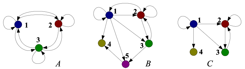
Any simple digraph $G$ is uniquely determined through one of its associated matrices, known as adjacency matrix $A_{G}$, whose element $a_{ij}$ is defined to be one if there exists an arrow joining vertex i with vertex j and zero otherwise. This is not the only possible characterization of graphs using matrices.

The incidence matrix is an $m\times n$ matrix $I^{m}_{n}$, where $m$ is the number of nodes and $n$ the number of edges, such that $I^{i}_{j}=-1$ if edge $e_{j}$ leaves the node and $I^{i}_{j}=1$ if edge $e_{j}$ enters the node ($I^{i}_{j}=0$ otherwise). As it is possible to relate the adjacency and incidence matrices through line graphs, we will mainly characterize graphs through their adjacency matrices.

In addition, a vector that we call node vector $V_{G}$ is associated to our digraph $G$, with its elements equal to one if the corresponding node is in $G$ and zero otherwise. $V_{G}$ will be necessary because we will study sequences of productions, which probably apply to different graphs. Their adjacency matrices will then refer to different sets of nodes. In order to operate algebraically we will complete all matrices (refer to Sec. 19 for completion). Node vectors are used to distinguish which nodes belong to the graph and which ones have been added for algebraic operation consistency. Next example illustrates this point.

Example.$\square$The adjacency matrices $A^{E}$ and $C^{E}$ for first and third graphs of Fig. 10 are:

$$A^{E}=\left[\begin{array}[]{ccccc}\vskip-6.0pt1&1&1&0&|\;1\\ \vskip-6.0pt1&1&1&0&|\;2\\ \vskip-6.0pt1&1&1&0&|\;3\\ \vskip-6.0pt0&0&0&0&|\;4\\ \end{array}\right]A^{N}=\left[\begin{array}[]{cc}\vskip-6.0pt1&|\;1\\ \vskip-6.0pt1&|\;2\\ \vskip-6.0pt1&|\;3\\ \vskip-6.0pt0&|\;4\\ \end{array}\right]C^{E}=\left[\begin{array}[]{ccccc}\vskip-6.0pt1&1&1&1&|\;1\\ \vskip-6.0pt0&1&1&0&|\;2\\ \vskip-6.0pt0&1&0&0&|\;3\\ \vskip-6.0pt0&0&0&0&|\;4\\ \end{array}\right]C^{N}=\left[\begin{array}[]{cc}\vskip-6.0pt1&|\;1\\ \vskip-6.0pt1&|\;2\\ \vskip-6.0pt1&|\;3\\ \vskip-6.0pt1&|\;4\\ \end{array}\right]$$

where $A^{N}$ and $C^{N}$ are the corresponding node vectors. A vertically separated column indicates node ordering, which applies both to rows and columns. Note that edges incident to node $4$ are considered in matrix $A^{E}$. As there is no node $4$ in $A$, corresponding elements in the adjacency matrix are zero. To clearly state that this node does not belong to graph $A$ we have a zero in the fourth position of $A^{N}$. $\blacksquare$

Note that simple graphs (without orientation on edges) can be studied if we limit to the subspace of symmetric adjacency matrices. In Sec. 43 we study how to extend Matrix Graph Grammars approach to consider multigraphs and multidigraphs. The difference between a simple digraph and a multidigraph is that simple graphs allow a maximum of one edge connecting two nodes in each direction, while a multidigraph allows a finite number of them.

In the literature, depending mainly on the book, there is some confusion with terminology. At times, the term graph applies to multigraphs while other times graph refers to simple graphs (also known as relational graphs). Whenever found in this book, and unless otherwise stated, the term graph should be understood as simple digraph.

The basic Boolean operations on graphs are defined component-wise on their adjacency matrices. Let $G$ and $H$ be two graphs with adjacency matrices $\left(g^{i}_{j}\right)$ and $\left(h^{i}_{j}\right)$, $i,j\in\{1,\ldots n\}$, then:

$$G\vee H=\left(g^{i}_{j}\vee h^{i}_{j}\right)\quad G\wedge H=\left(g^{i}_{j}\wedge h^{i}_{j}\right)\quad\overline{G}=\left(\overline{g^{i}_{j}}\right).$$

Similarly to ordinary matrix product based on addition and multiplication by scalars, there is a natural definition for a Boolean product with the same structure but using Boolean operations and and or.

Definition 6.1 (Boolean Matrix Product)

For digraphs $G$ and $H$, let $M_{G}=\left(g^{i}_{j}\right)_{i,j\in\{1,\ldots,n\}}$ and $M_{H}=\left(h^{i}_{j}\right)_{i,j\in\{1,\ldots,n\}}$ be their respective adjacency matrices. The Boolean product is an adjacency matrix again whose elements are defined by:

$$\left(M_{G}\odot M_{H}\right)^{i}_{j}=\bigvee_{k=1}^{n}\left(g^{i}_{k}\wedge h^{k}_{j}\right).$$ (2)

Element $(i,j)$ in the Boolean product matrix is one if there exists an edge joining node $i$ in digraph $G$ with some node $k$ in the same digraph and another edge in digraph $H$ starting in $k$ and ending in $j$. The value will be zero otherwise.

If for example we want to check whether node $j$ is reachable starting in node $i$ in $n$ steps or less, we may calculate $\bigvee_{k=1}^{n}A^{(k)}$, where $A^{(k)}=A\odot\stackrel{{\scriptstyle k)}}{{\cdots}}\odot A$, and see if element $(i,j)$ is one. We will consider square matrices only as every node can be either initial or terminal for any edge.

Another useful product operation that can be defined for two simple digraphs $G_{1}$ and $G_{2}$ is its tensor product (defined in Sec. 7) $G=G_{1}\otimes G_{2}$:

1. The nodes set is the Cartesian product $V(G)=V(G_{1})\times V(G_{2})$.

2. Two vertices’s $u_{1}\otimes u_{2}$ and $v_{1}\otimes v_{2}$ are adjacent if and only if $u_{1}$ is adjacent to $v_{1}$ in $G_{1}$ and $u_{2}$ is adjacent to $v_{2}$ in $G_{2}$.

In Sec. 7 we will see that the adjacency matrix of $G$ coincide with the tensor product of the adjacency matrices of $G_{1}$ and $G_{2}$.

Definition 6.3, Proposition 6.4 and the introduction above of the nodes vector is not standard in graph theory (in fact, as far as we know, we are introducing them). The decision of including them in this introductory section is because they are simple results very close with what one understands as “basics” of a theory.

Given an adjacency matrix and a vector of nodes, a natural question is whether they define a simple digraph or not.

Definition 6.2 (Compatibility)

A Boolean matrix $M$ and a vector of nodes $N$ are compatible if they define a simple digraph: No edge is incident to any node that does not belong to the digraph.

An edge incident to some node which does not belong to the graph (has a zero in the corresponding position of the nodes vector) is called a dangling edge.

In the DPO/SPO approaches, this condition is checked when building a direct derivation, known as dangling condition. The idea behind it is to obtain a closed set of entities, i.e. deletion of nodes outputs a digraph again (every edge is incident to some node). Proposition 6.4 below provides a criteria for testing compatibility for simple digraphs.

Definition 6.3 (Norm of a Boolean Vector)

Let $N=\left(v_{1},\ldots,v_{n}\right)$ be a Boolean vector. Its norm $\left\|\,\cdot\,\right\|_{1}$ is given by:

$$\left\|N\right\|_{1}=\bigvee_{i=1}^{n}v_{i}.$$ (3)

Proposition 6.4

A pair $\left(M,N\right)$, where $M$ is an adjacency matrix and $N$ a vector of nodes, is compatible if and only if

$$\left\|\left(M\vee M^{t}\right)\odot\overline{N}\right\|_{1}=0$$ (4)

where t denotes transposition.

Proof
$\square$In an adjacency matrix, row $i$ represents outgoing edges from vertex $i$, while column $j$ are incoming edges to vertex $j$. Moreover, $\left(M\right)_{ik}\wedge\left(\overline{N}\right)_{k}=1$ if and only if $\left(M\right)_{ik}=1$ and $\left(N\right)_{k}=0$, and thus the $i$-th element of vector $M\odot\overline{N}$ is one if and only if there is a dangling edge in row number $i$. We have just considered outgoing edges; for incoming ones we have a very similar term: $M^{t}\odot\overline{N}$. To finish the sufficient part of the proof – necessity is almost straightforward – we or both terms and take norms to detect if there is a $1$. $\blacksquare$

Remark.$\square$We have used in the proof of Proposition 6.4 distribution of $\odot$ and $\vee$, $\left(M_{1}\vee M_{2}\right)\odot M_{3}=\left(M_{1}\odot M_{3}\right)\vee\left(M_{2}\odot M_{3}\right)$. In addition, we also have the distributive law on the left, i.e. $M_{3}\odot\left(M_{1}\vee M_{2}\right)=\left(M_{3}\odot M_{1}\right)\vee\left(M_{3}\odot M_{2}\right)$. Besides, it will be stated without proof that $\left\|\,\omega_{1}\vee\omega_{2}\right\|_{1}=\left\|\,\omega_{1}\right\|_{1}\vee\left\|\,\omega_{2}\right\|_{1}$. $\blacksquare$

In Chap. id1 we will deal with matching, i.e. finding the left hand side of a graph grammar rule in the initial state (host graph). A matching algorithm is not proposed; our approach assumes that such algorithm is given. This is closely related to the well known graph-subgraph isomorphism problem (SI) which is an NP-complete decision problem if the number of nodes in the subgraph is strictly smaller than the number of nodes in the graph. We will brush over complexity theory in Chap. 51.

7 Tensor Algebra

Throughout the book, quantities that can be represented by a letter with subscripts or superscripts attached will be used, together with some algebraic structure (tensorial structure). This section is devoted to a quick introduction to this topic. Two very good references are [33] (with relations to physics) and the classic book [75].

A tensor is a multilinear application between vector spaces. It is at times interesting to stay at a more abstract level and think of a tensor as a system that fulfills certain notational properties. Systems can be heterogeneous when there are different types of elements, but we will only consider homogeneous systems. Therefore we will speak of systems or tensors, it does not matter which.

The rank of a system (tensor) is the number of indexes it has, taking into account whether they are superscripts or subscripts. For example, $A^{i}_{jk}$ is $\genfrac{[}{]}{0.0pt}{}{1}{2}$-valent or of rank (1,2). Subscripts or superscripts are referred to as indexes or suffixes.

Algebraic operations of addition and subtraction apply to systems of the same type and rank. They are defined component-wise, e.g. $C^{i}_{jk}=A^{i}_{jk}+B^{i}_{jk}$, provided that some additive structure is defined on elements of the system. We do not follow the Einstein summation convention, which states that when an index appears twice, one in an upper and one in a lower position, then they are summed up over all its possible values.

The product is obtained multiplying each component of the first system with each component of the second system, e.g. $C^{imnl}_{j}=A^{i}_{j}\otimes B^{mnl}$. Such a product is called outer product or tensor product. The rank of the result is the sum of the ranks of the factors and inherits all the indexes of its factors. All linear relations are satisfied, i.e. for $v_{1},v_{2}\in V$, $w\in W$ and $v\otimes w\in V\otimes W$ the following identities are fulfilled:

1. $(v_{1}+v_{2})\otimes w=v_{1}\otimes w+v_{2}\otimes w$.

2. $cv\otimes w=v\otimes cw=c(v\otimes w)$.

To categorically characterize tensor products note that there is a natural isomorphism between all bilinear maps from $E\times F$ to $G$ and all linear maps from $E\otimes F$ to $G$. $E\otimes F$ has all and only the relations that are necessary to ensure that a homomorphism from $E\otimes F$ to $G$ will be linear (this is a universal property). For vector spaces this is quite straightforward, but in the case of $R$-modules (modules over a ring $R$) this is normally accomplished by taking the quotient with respect to appropriate submodules.

Example.$\square$The Kronecker product is a special case of tensor product that we will use in Chap. id1. Given matrices $A=\left(a^{i_{1}}_{j_{1}}\right)_{m\times n}$ and $B=\left(b^{i_{2}}_{j_{2}}\right)_{p\times q}$, it is defined to be $C=A\otimes B=(c^{i}_{j})_{mp\times nq}$ where

$$c^{i}_{j}=a^{i_{1}}_{j_{1}}\cdot b^{i_{2}}_{j_{2}}$$ (5)

being $i=(i_{1}-1)n+i_{2}$ and $j=(j_{1}-1)m+j_{2}$. The notation $A=\left(a^{i}_{j}\right)_{m\times n}$ denotes a matrix with $m$ rows and $n$ columns, i.e. $i\in\{1,\ldots,m\}$ and $j\in\{1,\ldots,n\}$. As an example:

$$A=\left[\begin{array}[]{cc}a^{1}_{1}&a^{1}_{2}\end{array}\right]_{1\times 2}B=\left[\begin{array}[]{cc}b^{1}_{1}&b^{1}_{2}\\ b^{2}_{1}&b^{2}_{2}\end{array}\right]_{2\times 2}C=A\otimes B=\left[\begin{array}[]{cccc}a^{1}_{1}b^{1}_{1}&a^{1}_{1}b^{1}_{2}&a^{1}_{2}b^{1}_{1}&a^{1}_{2}b^{1}_{2}\\ a^{1}_{1}b^{2}_{1}&a^{1}_{1}b^{2}_{2}&a^{1}_{2}b^{2}_{1}&a^{1}_{2}b^{2}_{2}\end{array}\right]_{2\times 4}$$

Note that the Kronecker product of the adjacency matrices of two graphs is the adjacency matrix of the tensor product graph (see Sec. 6 for its definition). $\blacksquare$

The operation of contraction happens when an upper and a lower indexes are set equal and summed up, e.g. $C^{imnl}_{j}\longmapsto C^{mnl}=\sum_{j=1}^{N}C^{jmnl}_{j}=\sum_{i=j}C^{imnl}_{j}$. For example, the standard multiplication of a vector by a matrix is a contraction: Consider matrix $A^{i}_{j}$ and vector $v^{k}$ with $i,j,k\in\{1,\ldots,n\}$, then matrix multiplication can be performed by making $j$ and $k$ equal and summing up, $u^{i}=\sum_{j=1}^{n}A^{i}_{j}v^{j}$.

The inner product is represented by $\left\langle\,\cdot\,,\cdot\,\right\rangle$ and is obtained in two steps:

1. Take the outer product of the tensors.

2. Perform a contraction on two of its indexes.

In Sec. 8 we will extend this notation to cope with graph grammar rules representation.

Upper indexes are called contravariant and lower indexes covariant. Contravariance is associated to the tangent bundle (tangent space) of a variety and corresponds, so to speak, to columns. Covariance is the dual notion and is associated to the cotangent bundle (normal space) and rows. As an example, if we have a vector $V$ in a three dimensional space with basis $\left\{E_{1},E_{2},E_{3}\right\}$ then it can be represented in the form $A=a^{1}E_{1}+a^{2}E_{2}+a^{3}E_{3}$. Components $a^{i}$ can be calculated via $a^{i}=\left\langle A,E^{i}\right\rangle$ with $\left\langle E^{i},E_{j}\right\rangle=\delta^{i}_{j}$, where the Kronecker delta function is 1 if $i=j$ and zero if $i\neq j$. Basis $\left\{E^{i}\right\}$ and $\left\{E_{i}\right\}$ are called reciprocal or dual.

We will not enter the representation of $\delta$ in integral form or the relation with the Dirac delta function, of fundamental importance in distribution theory, functional analysis (see Sec. 8) and quantum mechanics. The Kronecker delta can be generalized to an $\genfrac{[}{]}{0.0pt}{}{n}{n}$-valent tensor:

$$\delta^{j_{1},\ldots,j_{n}}_{i_{1},\ldots,i_{n}}=\prod_{k=1}^{n}\delta_{i_{k}j_{k}}.$$ (6)

Besides the Kronecker delta, there are other very useful tensors such as the metric tensor, which can be informally introduced by $g^{ij}E_{i}=E^{j}$ and $g_{ij}E^{j}=E_{i}$. Note that $g$ raises or lowers indexes, thus moving from covariance to contravariance and vice versa. Related to $\delta$ and to group theory is the important Levi-Civita symbol:

$$\varepsilon_{\sigma}=\left\{\begin{array}[]{ll}+1&\qquad\textrm{if $\sigma$ is an even permutation.}\\ -1&\qquad\textrm{if $\sigma$ is an odd permutation.}\\ 0&\qquad\textrm{otherwise.}\\ \end{array}\right.$$ (7)

where $\sigma=(i_{1}\;\ldots\;i_{n})$ is a permutation of $(1\;\ldots\;n)$. See Sec. 9 for definitions and further results. Symbols $\delta$ and $\varepsilon$ can be related through matrix $A=(a_{kl})=\delta_{i_{k}j_{l}}$ and:

$$\varepsilon_{i_{1}\ldots}\varepsilon_{j_{1}\ldots}=det(A).$$ (8)

8 Functional Analysis

Functional analysis is a branch of mathematics focused on the study of functions – operators – in infinite dimensional spaces (although its results also apply to finite dimensional spaces). Besides the algebraic structure (normally a vector space but at times groups) some other ingredients are normally added such as an inner product (Hilbert spaces), a norm (Banach spaces) a metric (metric spaces) or just a topology (topological vector spaces).

An operator is just a function, but the term is normally employed to call attention to some special aspect. Examples of operators in mathematics are differential and integral operators, linear operators (linear transformations), Fourier transform, etc.

In this book we will call operators to functions that act on functions with image a function. Operators will be used, e.g. in Chap. id1 to modify productions in order to get a production or a sequence of productions.

We will need to change productions as commented above and our inspiration comes from operator theory and functional analysis, but we would like to put it forward in a quantum mechanics style. So, although it will not be used as it is, we will give a very brief introduction to Hilbert and Banach spaces, bra-ket notation and duality.

A Hilbert space $\mathcal{H}$ is a vector space, complete with respect to Cauchy sequences over a field $K$ (every Cauchy sequence has a limit in $\mathcal{H}$), plus a scalar (or inner) product. Completeness ensures that the limit of a convergent sequence is in the space, facilitating several definitions from analysis (note that a Hilbert space can be infinite-dimensional). The inner product – $\left\langle u,v\right\rangle$, $u,v\in\mathcal{H}$ – equips the structure with the notions of distance and angle (in particular perpendicularity). From a geometric point of view, the scalar product can be interpreted as a projection whereas analytically it can be seen as an integral.

The inner product gives raise to a norm $\left\|\,\cdot\right\|$ via $\left\|x\right\|^{2}=\left\langle x,x\right\rangle$, $\forall x\in\mathcal{H}$. Any norm can be interpreted as a measure of the size of elements in the vector space. Every inner product defines a norm but, in general, the opposite is not true, i.e. norm is a weaker concept than scalar product.

The relationship between row and column vectors can be generalized from an abstract point of view through dual spaces. The dual space $\mathcal{H}^{*}$ of a Hilbert space $\mathcal{H}$ over the field $K$ has as elements $x^{*}\in\mathcal{H}^{*}$, linear applications with domain (initial set) $\mathcal{H}$ and codomain (image) the underlying field $K$, $x^{*}:\mathcal{H}\rightarrow K$.

The dual space becomes a vector space defining the addition $\forall x_{1}^{*},x_{2}^{*}\in\mathcal{H}^{*}$, $x\in\mathcal{H}$ by $(x_{1}^{*}+x_{2}^{*})(x)=x_{1}^{*}(x)+x_{2}^{*}(x)$ and the scalar product $\forall k\in K$ by $kx^{*}(x)=x^{*}(kx)$. Using tensor algebra terminology (see Sec. 7) elements of $\mathcal{H}$ are called covariant and elements of $\mathcal{H}^{*}$ contravariant. Note how in $\left\langle x,y\right\rangle$ it is possible to think of $x$ as an element of the vector space and $y$ as an element of the dual space.

Any Hilbert space is isomorphic (or anti-isomorphic) to its dual space, $\mathcal{H}\cong\mathcal{H}^{*}$, which is the content of the Riesz representation theorem. This is particularly relevant to us because it is a justification of the Dirac bra-ket notation that we will also use.

The Riesz representation theorem can be stated in the following terms: Let $\mathcal{H}$ be a Hilbert space, $\mathcal{H}^{*}$ its dual and define $\phi_{x}(y)=\left\langle x,y\right\rangle$, $\phi\in\mathcal{H}^{*}$. Then, the mapping $\Phi:\mathcal{H}\rightarrow\mathcal{H}^{*}$ such that $x\mapsto\phi_{x}$ is an isometric isomorphism. This means that $\Phi$ is a bijection and that $\left\|x\right\|=\left\|\phi_{x}\right\|$.

We will very briefly introduce Banach spaces to illustrate how notions and ideas from Hilbert spaces, specially notation, is extended in a more or less natural way.

A complete vector space plus a norm is known as a Banach space, $\mathcal{B}$. Associated to any Banach space there exists its dual space, $\mathcal{B}^{*}$, defined as before. Contrary to Hilbert spaces, a Banach space is not isometrically isomorphic to its dual space.

It is possible to define a distance (also called metric) out of a norm: $d(x,y)=\left\|x-y\right\|$. Even though there is no such geometrical intuition of projection nor angles, it is still possible to use the notation we are interested in. Given $x\in\mathcal{B},x^{*}\in\mathcal{B}^{*}$, instead of writing $x^{*}\left(x\right)$ (the result is an element of $\mathcal{K}$) at times $\left\langle x,x^{*}\right\rangle$ is preferred. Although the space and its dual live at different levels, we would like to recover this geometrical intuition of projection. In some (very nice) sense, the result of $x^{*}\left(x\right)$ is the projection of $x$ over $x^{*}$.

The same applies for an operator $T$ acting on a Banach space $\mathcal{B}$, $T:\mathcal{B}\rightarrow\mathcal{B}$. Suppose $f,g\in\mathcal{B}$, then $g=T\left(f\right)\equiv\left\langle f,T\right\rangle$. This is closer to our situation, so the application of a production can be written

$$R=\left\langle L,p\right\rangle.$$ (9)

The left part is sometimes called bra and the right part ket: $\left\langle bra,ket\right\rangle$.

Besides dual elements, the adjoint of an operator is also represented using asterisks. In our case, the adjoint operator of $T$, represented by $T^{*}$, is formally defined by the identity:

$$\left\langle\,L,Tp\,\right\rangle=\left\langle\,T^{*}L,p\,\right\rangle.$$ (10)

Roughly speaking, $T$ is an operator (a function) that modifies a production, being its output a production again, so the left hand side in (10) is equivalent to $T\left(p\right)\left(L\right),$ and the right hand side is just $p\left(T^{*}L\right)$. Note that $T\left(p\right)$ is a production and $T^{*}L$ is a simple digraph.

In quantum mechanics the possible states of a quantum mechanical system are represented by unit vectors – state vectors – in a Hilbert space $\mathcal{H}$ or state space (equivalently, points in a projective Hilbert space). Each observable – property of the system – is defined by a linear operator acting on the elements of the state space. Each eigenstate of an observable corresponds to an eigenvector of the operator and the eigenvalue to the value of the observable in that eigenstate. An interpretation of $\left\langle\psi|\,\phi\right\rangle$ is the probability amplitude for the state $\psi$ to collapse into the state $\phi$, i.e. the projection of $\psi$ over $\phi$. In this case, the notation can be generalized to metric spaces, topological vector spaces and even vector spaces without any topology (close to our case as we will deal with graphs without introducing notions such as metrics, scalar products, etc). Two recommended references are [37] and [68].

This digression on quantum mechanics is justified because along the present contribution we would like to think in graph grammars as having a static definition which provokes a dynamic behaviour and the duality between state and observable. Besides, the use of the notation, we would like to keep some “physical” (mechanics) intuition whenever possible.

9 Group Theory

One way to introduce group theory is to define it as the part of mathematics that study those structures for which the equation $a\cdot x=b$ has a unique solution. There is a very nice definition due to James Newman [57] that I’d like to quote:

The theory of groups is a branch of mathematics in which one does something to something and then compares the results with the result of doing the same thing to something else, or something else to the same thing.

We will be interested in groups, mainly in its notation and basic results, when dealing with sequentialization in Chaps. id1 and id1. A group $G$ is a set together with an operation $\left(G,\cdot\right)$ that satisfies the following axioms:

1. Closure: $\forall a,b\in G$, $a\cdot b\in G$.

2. Associativity: $\forall a,b,c\in G$, $a\cdot(b\cdot c)=(a\cdot b)\cdot c$.

3. Identity element: $\exists e\in G$ such that $a\cdot e=e\cdot a=a$.

4. Inverse element: $\forall a\in G$ $\exists b\in G$ such that $a\cdot b=e=b\cdot a$.

Actually, the third and fourth axioms can be weakened as only one identity per axiom should suffice, but we think it is worth stressing the fact that if they exist then they work on both sides. Normally, the inverse element of $a$ is written $a^{-1}$. At times the identity element is represented by $1_{G}$ or $0_{G}$, depending on the notation (Abelian or non-Abelian). A group is called Abelian or commutative if $\forall a,b\in G$, $a\cdot b=b\cdot a$.

A group $S$ inside a group $G$ is called a subgroup. If this is the case, we need $S$ to be closed under the group operation, it also must have the identity element $e$ and every element in $S$ must have an inverse in $S$. If $S\subset G$ and $\forall a,b\in S$ we have that $a\cdot b^{-1}\in S$ then $S$ is a subgroup. Lagrange’s theorem states that the order of a subgroup (number of elements) necessarily divides the order of the group.

We are almost exclusively interested in groups of permutations: For a given sorted set, a change of order is called a permutation. This does not reduce the scope because, by Cayley’s theorem, every group is isomorphic to some group of permutations.

A transposition is a permutation that exchanges the position of two elements whilst leaving all other objects unmoved. It is known that any permutation is equivalent to a product of transpositions. Furthermore, if a permutation can result from an odd number of transpositions then it can not result from and even number of permutations, and vice versa. A permutation is even if it can be produced by an even number of exchanges and odd in the other case. This is called parity.

The signature of a permutation $\sigma$, $sgn(\sigma)$, is $+1$ if the permutation is even and $-1$ if it is odd. This is the Levi-Civita symbol as introduced in Sec. 7 if it is extended for non-injective maps with value zero.

Any permutation can be decomposed into cycles. A cycle is a closed chain inside a permutation (so it is a permutation itself) which enjoys some nice properties among which we highlight:

• Cycles inside a permutation can be chosen to be disjoint.

• Disjoint cycles commute.

Any permutation can be written as a two row matrix where the first row represents the original ordering of elements and the second the order once the permutation is applied.

Example.$\square$The permutation $\sigma$ can be decomposed into the product of three cycles:

$$\sigma=\left[\begin{array}[]{cccccccc}1&2&3&4&5&6&7&8\\ 3&5&7&8&2&4&1&6\end{array}\right]=(1\;3\;7)(2\;5)(4\;8\;6).$$

Note that this decomposition is not unique because any decomposition into transpositions would do (and there are infinitely many). $\blacksquare$

If the permutation turns out to be a cycle, then a clearer notation can be used: Write in a row, in order, the following element in the permutation. In the example above we begin with 1 and note that 1 goes to 3, which goes to 7, which goes back to 1 and hence it is written $(1\;3\;7)$.

A cycle with an even number of elements is an odd permutation and a cycle with an odd number of elements is an even permutation. In practice, in order to determine whether a given permutation is even or odd, one writes the permutation as a product of disjoint cycles: The permutation is odd if and only if this factorization contains an odd number of even-length cycles.

10 Summary and Conclusions

In this chapter we have quickly reviewed some basic facts of mathematics that will be used throughout the rest of the book: The basics of first order, second order and monadic second order logics, some constructions of category theory such as pushouts and pullbacks together with the introduction of some categories, graph theory basic definitions and compatibility, tensor algebra and functional analysis notations and some basic group theory, paying some attention to permutations.

Internet is full of very good web pages introducing these branches of mathematics with deeper explanations and plenty of examples. It is not possible to give an exhaustive list of all web pages visited to make this chapter. Nevertheless, I would like to highlight the very good job being performed by the community at http://planetmath.org/ and http://www.wikipedia.org/.

Next chapter summarizes current approaches to graph grammars and graph transformation systems, so it is still introductory. We will put our hands on Matrix Graph Grammars in Chap. id1.

Chapter Graph Grammars Approaches

Before moving to Matrix Graph Grammars it is necessary to take a look at other approaches to graph transformation to “get the taste”, which is the aim of this chapter. We will see the basic foundations leaving comparisons of more advanced topics (like application conditions) to sporadic remarks in future chapters.

Sections 11 and 12 are devoted to categorical approaches, probably the most developed formalizations of graph grammars. On the theoretical side, very nice ideas have put at our disposal the possibility of using category theory and its generalization power to study graph grammars, but even more so, a big effort has been undertaken in order to fill the gap between category theory and practice with tools such as AGG (see [22]). Please, refer to [1] for a detailed discussion and comparison of tools.

In Secs. 13 and 14 two completely different formalisms to the categorical approach are summarized, at times called set-theoretic or even algorithmic approaches. They are in some sense closer to implementation than those using category theory. There has been a lot of research in these two essential approaches so unfortunately we will just scratch the surface.

Interestingly, it is possible to study graph transformation using logics, providing us with all powerful methods from this branch of mathematics, monadic second order logics in particular. We will brush over this brilliant approach in Sec. 15.

To finish this review we will briefly touch on the very interesting relation-algebraic approach in Sec. 16, which has not attracted as much attention as one should expect. Finally, the chapter is closed with a summary in Sec. 17.

In this chapter we abuse of bold letters with the intention of facilitating the search of some definition or result. It is assumed that this chapter as well as Chap. id1 will be mainly used for reference.

11 Double PushOut (DPO)

11.1 Basics

In the DPO approach to graph rewriting, a direct derivation is represented by a double pushout in category Graph (multigraphs and total graph morphisms). Productions can be defined as three graph components, separating the elements that should be preserved from the left and right hand sides of the rule.

A production $p:(L\overset{l}{\longleftarrow}K\overset{r}{\longrightarrow}R)$ consists of a production name $p$ and a pair of injective graph morphisms $l\colon K\rightarrow L$ and $r\colon K\rightarrow R$. Graphs $L$, $R$ and $K$ are respectively called the left-hand side (LHS), right-hand side (RHS) and the interface of $p$. Morphisms $l$ and $r$ are usually injective and can be taken to be inclusions without loss of generality.

Figure 11: Example of Simple DPO Production

The interface $K$ of a production consists of the elements that should be preserved by the production application, while elements in $L-K$ are deleted and elements of $R-K$ are added. Figure 11 shows a simple DPO production named del, that can be applied if a path of three nodes is found. If so, the production eliminates the last node and all edges and creates a loop edge in the second node.

A direct derivation can be defined as an application of a production to a graph through a match by constructing two pushouts. A match is a total morphism from the left hand side of the production onto the host graph, i.e. it is the operation of finding the LHS of the grammar rule in the host graph. Thus, given a graph $G$, a production $p:(L\overset{l}{\longleftarrow}K\overset{r}{\longrightarrow}R)$ and a match $m\colon L\rightarrow G$, a direct derivation from $G$ to $H$ using $p$ (based on $m$) exists if and only if the diagram in Fig. 12 can be constructed, where both squares are required to be pushouts in category Graph.

In Fig. 12, red dotted arrows represent the morphisms that must be defined in order to close the diagram, i.e. to construct the pushouts. $D$ is called the context graph. In particular, if the context graph can not be constructed then the rule can not be applied.

A direct derivation is written $G\overset{p,m}{\Longrightarrow}H$ or simply $G\Longrightarrow H$ if the production and the matching are known from context.

Figure 12: Direct Derivation as DPO Construction

For example, figure 11 shows the application of rule del to a graph. Morphisms $m$, $d$ and $m^{*}$ are depicted by showing the correspondence of the vertexes in the production and the graph.

In order to apply a production to a graph $G$, a pushout complement has to be calculated to obtain graph $D$. The existence of this pushout complement is guaranteed if the so-called dangling and identification conditions are satisfied. The first one establishes that a node in $G$ cannot be deleted if this causes dangling edges. The second condition states that two different nodes or edges in $L$ cannot be identified (by means of a non-injective match) as a single element in $G$ if one of the elements is deleted and the other is preserved. Moreover, the injectivity of $l\colon K\rightarrow L$ guarantees the uniqueness of the pushout complement. The identification condition plus the dangling condition is at times known as gluing condition.

In the example in Fig. 11 the match $(1,2,3)\mapsto(a,b,c)$ does not fulfill the dangling condition, as the deletion of node $d$ would make edges $(a,c)$ and $(c,d)$ become dangling, so the production cannot be applied at this match. One example (for SPO, but it can be easily translated into DPO) in which the identification condition fails is depicted to the right of Fig. 17 on p. 17.

11.2 Sequentialization and Parallelism

A graph grammar can be defined as $\mathcal{G}=\langle(p:L\overset{l}{\longleftarrow}K\overset{r}{\longrightarrow}R)_{p\in P},G_{0}\rangle$ (see [11], Chap. 3), where $(p:L\overset{l}{\longleftarrow}K\overset{r}{\longrightarrow}R)_{p\in P}$ is a family of productions indexed by their names and $G_{0}$ is the starting graph of the grammar. The semantics of the grammar are all reachable graphs that can be obtained by successively applying the rules in $\mathcal{G}$. Events changing a system state can thus be modeled using graph transformation rules.

In real systems, parallel actions can take place. Two main approaches can be followed in order to describe and analyze parallel computations. In the first one, parallel actions are sequentialized, giving rise to different interleavings (for example a single CPU simulating multitasking). In the second approach, called explicit parallelism, actions are really simultaneous (for example more than one CPU performing several tasks).

Figure 13: Parallel Independence

In the interleaving approach, two actions (rule applications) are considered to be parallel if they can be performed in any order yielding the same result. This can be understood in two different ways.

The first interpretation is called parallel independence and states that two alternative direct derivations $H_{1}\overset{p_{1}}{\Longleftarrow}G\overset{p_{2}}{\Longrightarrow}H_{2}$ are independent if there are direct derivations such that $H_{1}\overset{p_{2}}{\Longrightarrow}X\overset{p_{1}}{\Longleftarrow}H_{2}$ (see Fig. 13). That is, both derivations are not in conflict, but one can be postponed after the other. It can be characterized using morphisms in a categorical style saying that two direct derivations (as those depicted in Fig. 13) are parallel independent if and only if

$$\exists i:L_{1}\rightarrow D_{2},j:L_{2}\rightarrow D_{1}\;|\;l^{*}_{2}\circ i=m_{1},l^{*}_{1}\circ j=m_{2}.$$ (11)

If one element is preserved by one derivation, but deleted by the other, then the latter is said to be weakly parallel independent of the first (it is characterized in equation 14). Thus, parallel independence can be defined as mutual weak parallel independence.

On the other hand (the second interpretation), two direct derivations are called sequential independent if they can be performed in different order with no changes in the result. That is, both $G\overset{p_{1}}{\Longrightarrow}H_{1}\overset{p_{2}}{\Longrightarrow}X$ and $G\overset{p_{2}}{\Longrightarrow}H_{2}\overset{p_{1}}{\Longrightarrow}X$ yield the same result (see Fig. 14). Again, categorically we say that two derivations are sequential independent if and only if

$$\exists i:R_{1}\rightarrow D_{2},j:L_{2}\rightarrow D_{1}\;|\;l^{*}_{2}\circ i=m^{*}_{1},r^{*}_{1}\circ j=m_{2}.$$ (12)

Mind the similarities with confluence (problem 5) and local confluence.

Figure 14: Sequential Independence

The conditions for sequential and parallel independence are given in the Local Church-Rosser Theorem [11], Chaps. 3 and 4. It says that two alternative parallel derivations are parallel independent if their matches only overlap in items that are preserved. Two consecutive direct derivations are sequential independent if the match of the second does not depend on elements generated by the first, and the second derivation does not delete an item that has been accessed by the first. Moreover, if two direct alternative derivations are parallel independent, their concatenation is sequential independent and vice versa.

The explicit parallelism view [11, 2] abstracts from any application order (no intermediate states are produced). In this approach, a derivation is modeled by a single production, called parallel production. Given two productions, $p_{1}$ and $p_{2}$, the parallel production $p_{1}+p_{2}$ is the disjoint union of both. The application of such production is denoted as $G\overset{p_{1}+p_{2}}{\Longrightarrow}X$.

Two problems arise here: The sequentialization of a parallel production (analysis), and the parallelization of a derivation (synthesis). In DPO, the parallelism theorem states that a parallel derivation $G\overset{p_{1}+p_{2}}{\Longrightarrow}X$ can be sequentialized into two derivations ($G\overset{p_{1}}{\Longrightarrow}H_{1}\overset{p_{2}}{\Longrightarrow}X$ and $G\overset{p_{2}}{\Longrightarrow}H_{2}\overset{p_{1}}{\Longrightarrow}X$) that are sequential independent. Conversely, two derivations can be put in parallel if they are sequentially independent.

This is a limiting case of amalgamation, which specifies that if there are two productions $p_{1}$ and $p_{2}$, then the amalgamated production $p_{1}\oplus_{p_{0}}p_{2}$ is defined such that the production $p_{1}$ and $p_{2}$ can be applied in parallel and the amalgamated production $p_{0}$ (that represents common parts of both) should be applied only once.

The concurrency theorem deals with the concurrent execution of productions that need not be sequentially independent. Hence, according to previous results, it is not possible to apply them in parallel. Anyway, they can be applied concurrently using a so-called $E$-concurrent graph production, $p_{1}*_{E}p_{2}$. We will omit the details, which can be consulted in [22].

Let the sequence $G\stackrel{{\scriptstyle p_{1},m_{1}}}{{\Longrightarrow}}H_{1}\stackrel{{\scriptstyle p_{2},m_{2}}}{{\Longrightarrow}}H_{2}$ be given. It is possible to construct a direct derivation $G\stackrel{{\scriptstyle p_{1}*_{E}p_{2}}}{{\Longrightarrow}}H_{2}$. The basic idea is to relate both productions through an overlapping graph $E$, which is a subgraph of $H_{1}$, $E=m^{*}_{1}(R_{1})\cup m_{2}(L_{2})$. The corresponding restrictions $\overline{m^{*}_{1}}:R_{1}\rightarrow E$ and $\overline{m_{2}}:L_{2}\rightarrow E$ of $m^{*}_{1}$ and $m_{2}$, respectively, must be jointly surjective. Also, any direct derivation $G\stackrel{{\scriptstyle p_{1}*_{E}p_{2}}}{{\Longrightarrow}}H_{2}$ can be sequentialized.

11.3 Application Conditions

We will make a brief overview of graph constraints and application conditions. In [14], graph constraints and application conditions were developed for the Double Pushout (DPO) approach to graph transformation and generalized to adhesive HLR categories in [22]. Atomic constraints were defined to be either positive or negative. A positive atomic graph constraint $PC\left(c\right)$ (where $c$ is an arbitrary morphism $c\colon P\rightarrow C$) is satisfied by graph $G$ if $\forall\,m_{P}\colon P\rightarrow G$ injective morphism there exists some $m_{C}\colon C\rightarrow P$ injective morphism such that $m_{P}=m_{C}\circ c$, mathematically written $G\models PC\left(c\right)$ (see left part of Fig. 15). It can be interpreted as graph $C$ must exist in $G$ if graph $P$ is found in $G$.

Graph morphism $m_{L}:L\rightarrow G$ satisfies the positive atomic application condition $P\left(c,\bigvee_{1}^{n}c_{i}\right)$ (with $c\colon L\rightarrow P$ and $c_{i}\colon P\rightarrow C_{i}$) if assuming $G\models PC\left(c\right)$, for all associated morphisms $m_{P}\colon P\rightarrow G,\exists\,m_{C_{i}}\colon C_{i}\rightarrow G$ such that $G\models PC\left(c_{i}\right)$. The notation used is $m_{L}\models P\left(c,\bigvee_{1}^{n}c_{i}\right)$, having also a similar interpretation to that of graph constraints: Suppose $L$ is found in $G$, if $P$ is also in $G$ then there must be some $C_{i}$ in $G$. Refer to the diagram on the right side of Fig. 15. A positive graph constraint is a Boolean formula over positive atomic graph constraints. Positive application conditions, negative application conditions and negative graph constraints are defined similarly.

Figure 15: Generic Application Condition Diagram

Finally, an application condition $AC\left(p\right)=\left(A_{L},A_{R}\right)$ for a production $p:L\rightarrow R$ consists of a left application condition $A_{L}$ over $L$ (also known as precondition) and a right application condition or postcondition $A_{R}$ over $R$. A graph transformation satisfies the application condition if the match satisfies $A_{L}$ and the comatch satisfies $A_{R}$. In [14, 32] it is shown that graph constraints can be transformed into postconditions which eventually can be translated into preconditions. In this way, it is possible to ensure that starting with a host graph that meets certain restrictions, the application of the production will output a graph that still satisfies the same restrictions.

DPO approach has been embedded in the weak adhesive HLR categorical approach, which we will shortly review in the following subsection.

11.4 Adhesive HLR Categories

This section finishes with a celebrated generalization of DPO. It was during 2004 that adhesive HLR categories were defined by merging two striking ideas: Adhesive categories [43] and high level replacement systems [16, 17]. See Sec. 5 for a quick overview of category theory.

Basic definitions are extended almost immediately to adhesive HLR systems $(\mathcal{C},\mathcal{M})$. A production $p:(L\overset{l}{\longleftarrow}K\overset{r}{\longrightarrow}R)$ consists of three objects $L$, $K$ and $R$, the left hand side, the gluing object and the right hand side, respectively, and morphisms $l:K\rightarrow L$ and $r:K\rightarrow R$ with $l,r\in\mathcal{M}$. There is a slight change in notation and the term derivation is substituted by transformation, and direct derivation by direct transformations. Adhesive HLR grammars and languages are defined in the usual way.

In order to apply a production we have to construct the pushout complement and a necessary and sufficient condition for it is the gluing condition. For adhesive HLR systems this is possible if we can construct initial pushouts, which is an additional requirement (it does not follow from the axioms of adhesive HLR categories): A match $m:L\rightarrow G$ satisfies the gluing condition with respect to a production $p:(L\overset{l}{\longleftarrow}K\overset{r}{\longrightarrow}R)$ if for the initial pushout over $m$ in Fig. 16 there is a morphism $\overline{f}:X\rightarrow K$ such that $r\circ\overline{f}=f$.

Figure 16: Gluing Condition

Parallel and sequential independence are defined analogously to what has been presented in Sec. 11 and the local Church-Rosser and the parallelism theorems remain valid.

12 Other Categorical Approaches

This section presents other categorical approaches such as single pushout (SPO) and pullback and compares them with DPO (Sec. 11).

In the single pushout approach (SPO) to graph transformation, rules are modeled with two component graphs ($L$ and $R$) and direct derivations are built with one pushout (which performs the gluing and the deletion). SPO relies on category Graph^P of graphs and partial graph morphisms.

A SPO production $p$ can be defined as $p:(L\overset{r}{\rightarrow}R)$, where $r$ is an injective partial graph morphism. Those elements for which there is no image defined are deleted, those for which there is image are preserved and those that do not have a preimage are added.

A match for a production $p$ in a graph $G$ is a total morphism $m\colon L\rightarrow G$. Given a production $p$ and a match $m$ for $p$ in $G$, the direct derivation from $G$ is the pushout of $p$ and $m$ in Graph^P. As in DPO, a derivation is just a sequence of direct derivations.

The left part of Fig. 17 shows an example of the rule in Fig. 11, but expressed in the SPO approach. The production is applied to the same graph $G$ as in Fig. 12 but at a different match.

An important difference with respect to DPO is that in SPO there is no dangling condition: Any dangling edge is deleted (so rules may have side effects). In this example, node $c$ and edges $(a,c)$ and $(c,d)$ are deleted. In addition, in case of a conflict with the identification condition due to a non-injective matching, the conflicting elements are deleted.

Figure 17: SPO Direct Derivation

Due to the way in which SPO has been defined, even though the matching from the LHS into the host graph is a total morphism, the RHS matching can be a partial morphism (see the example to the right of Fig. 17).

In order to guarantee that all matchings are total it is necessary to ask for the conflict-free condition: A total morphism $m:L\rightarrow G$ is conflict free for a production $p:L\rightarrow R$ if and only if

$$m(x)=m(y)\implies\left[x,y\in dom(p)\textrm{ or }x,y\not\in dom(p)\right].$$ (13)

Results for explicit parallelism are slightly different in SPO. In this approach, a parallel direct derivation $G\overset{p_{1}+p_{2}}{\Longrightarrow}X$ can be sequentialized into $G\overset{p_{1}}{\Longrightarrow}H_{1}\overset{p_{2}}{\Longrightarrow}X$ if $G\overset{p_{2}}{\Longrightarrow}H_{2}$ is weakly parallel independent of $G\overset{p_{1}}{\Longrightarrow}H_{1}$ (and similarly for the other sequentialization). So as this condition may not hold, there are parallel direct derivations that do not have an equivalent interleaving sequence.

Figure 18: SPO Weak Parallel Independence

These conditions will be written explicitly because we will make a comparison in Sec. 32. Derivation $d_{1}$ is weakly parallel independent of derivation $d_{2}$ (see Fig. 18) if

$$m(L_{2})\cap m_{1}\left(m_{1}\backslash dom(p_{1})\right)=\emptyset.$$ (14)

Figure 19: SPO Weak Sequential Independence

There is an analogous concept, similarly defined, known as weak sequential independence. Let $d_{1}$ and $d_{2}$ be as defined in Fig. 19, then $d_{2}$ is weakly sequentially independent of $d_{1}$ if

$$m_{2}\left(L_{2}\right)\cap m^{*}_{1}\left(R_{1}\backslash p_{1}(L_{1})\right)=\emptyset.$$ (15)

If additionally

$$m^{*}_{1}\left(R_{1}\right)\cap m_{2}\left(L_{2}\backslash dom(p_{2})\right)=\emptyset$$ (16)

then $d_{2}$ is sequentially independent of $d_{1}$.

It is possible to synthesize both concepts (weak sequential independence and parallel independence) in a single diagram. See Fig. 20.

Figure 20: Sequential and Parallel Independence.

Due to the fact that approaches based on the pushout construction can not replicate substructures naturally, Bauderon and others have proposed a different setting by using pullbacks instead of pushouts [4, 5, 3]. We will call them SPB and DPB approaches, depending on the number of pullbacks, similarly to SPO and DPO.

Note that pullbacks are sub-objects of products (see Sec. 5) and that products are (in some sense) a natural replication mechanism. It has been shown that pullback approaches are strictly more expressive than those using pushouts, but they have some drawbacks as well:

1. The existence condition for pullback complements is much more complicated than with pushouts (gluing condition).

2. In general, this condition can not be treated with computers [36].

3. There is a loss in comprehensibility and intuitiveness.

In Fig. 21 what we understand by a replication that can be handled easily with SPB but not with SPO is illustrated. The pullback construction is depicted in dashed red color on the same production, which is drawn twice. To the left, the production on top with the morphism back to front (its LHS on the right and vice versa) and the system evolves from left to right (as in SPO or DPO), i.e. the initial state is $H_{1}$ and the final state is $H_{2}$.

To the right of the same figure the production is represented more naturally for us (the left hand side on the left and the right hand side on the right) but on the bottom of the figure. The system evolves on top from right to left (it should be more intuitive if it evolved from left to right). Besides, we notice that what we understand as the initial state is now given by the RHS of the production while the final state is given by the left hand side.

Figure 21: SPB Replication Example

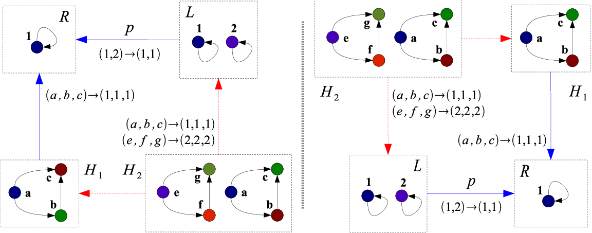
13 Node Replacement

Node Replacement grammars [23] (Chap. 1) are a class of graph grammars based on the replacement of nodes in a graph. The scheme is similar to the one described in Sec. 1, on p. 1 but with some peculiarities and notational changes. There is a mother graph (LHS, normally it consists of a single node) and a daughter graph (RHS) together with a gluing construction that defines how the daughter graph fits in the host graph once the substitution is carried out. Nodes of the mother graph play a similar role to non-terminals in Chomsky grammars. The differences among different node replacement grammars reside in the way the gluing is performed.

We will start with NLC grammars (Node Label Controlled, [23], Chap. 1) which are defined as the 5-tuple

$$G=(\Sigma,\Delta,P,C,S)$$ (17)

where $\Sigma$ are all node labels (alphabet set), $\Delta$ are node labels ($\Delta\subseteq\Sigma$) that do not appear on the LHS of any production (alphabet set of terminals, so non-terminals are $\Sigma-\Delta$), $P$ is the set of productions, $C$ are the gluing conditions (connection constructions) and $S$ is the initial graph.

Here only node labels matter. Each production is defined as a non-terminal node producing a graph with terminals and non-terminals along with a set of connection instructions. For example, in Fig. 22 we see a production $p$ with $X$ in its LHS and a subgraph in its RHS along with a connection relation $c$ in the box.

Production application (its semantics, also in Fig. 22) consists of deleting the LHS from the host graph, add the RHS and finally connect the daughter graph with the start graph. There are no application conditions.

Figure 22: Example of NLC Production

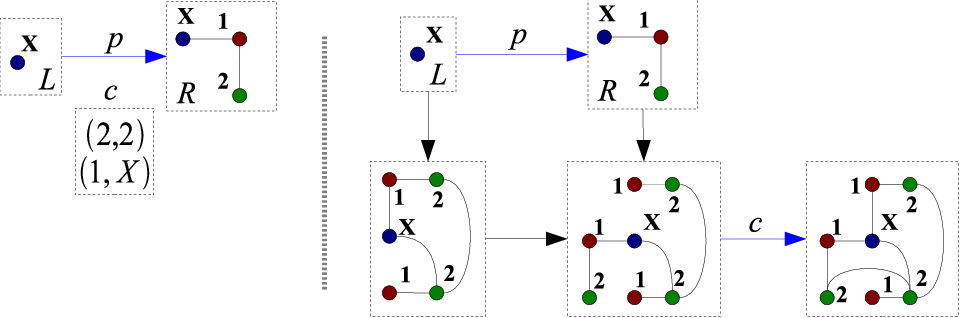
The linking part is performed according to a connection relation, which is a pair of node labels of the form $(x,y)$: If the left hand side node was adjacent to a node labeled $x$ then all nodes in the RHS with label $y$ will be adjacent to it.

NLC is a class of context-free graph grammars, in particular recursively defined properties can be described. Also, they are completely local and have no application conditions which allows to model derivations by derivation trees. However, the yield of a derivation tree is dependent on the order in which productions are applied. This property is known as confluence (see problem 5) and the subclass of NLC grammars that are confluent is called C-NLC.

At times it is desirable to refer to a concrete node instead of to a whole family in the gluing instructions. This variation is known as NCE grammar (Neighborhood Controlled Embedding) and is formally defined to be the tuple

$$G=(\Sigma,\Delta,P,S)$$ (18)

where $\Sigma$, $\Delta$ and $S$ are defined as above but productions in set $P$ are different.

The grammar rule $p:X\rightarrow(D,C)$ contains the production $p:X\rightarrow D$ and the connection $C$. The connection is of the form $(u,x)$ where $u$ is a label and $x$ is a particular node in the daughter graph. Note that NCE graph grammars are still NLC-like grammars, at least concerning replacement.

NCE can be extended in several ways but the most popular one is adding labels and a direction to edges, giving rise to edNCE grammars. Productions in edNCE are equal to those in NCE but connections differ a little bit, being of the form

$$(\mu,p/q,x,d),$$ (19)

where $\mu$ is a node label, $p$ and $q$ are edge labels, $x$ is a node of $D$ and $d\in\{in,out\}$ (which specifies the direction of the edge). For example, if $d=in$ the connection in eq. (19), it specifies that the embedding process should establish an edge with label $q$ to node $x$ of $D$ from each $\mu$-labeled $p$-neighbor of $m\in M$ (the mother graph) that is an in-neighbor of $m$.

The expressive power of edNCE is not increased neither if grammar rules change directions of edges nor if connection instructions make use of multiple edges.

The graphical representation differs a little from that of DPO and SPO. The daughter graph $D$ is included in a box and the area surrounding it represents its environment. Non-terminal symbols are represented by capital letters inside a small box (the large box itself can be viewed as a non-terminal symbol). Connection instructions are directed lines that connect nodes inside (new labels) with nodes outside (old labels).

Figure 23: edNCE Node Replacement Example

Example.$\square$The notation $G=H_{2}[n/H_{1}]$ is employed for a derivation, meaning that graph $G$ is obtained by making the substitution $n\mapsto H_{1}$ in $H_{2}$, i.e. by replacing node $n$ in $H_{2}$ with graph $H_{1}$. In the example of Fig. 23 (with non-terminal node $N$) we have substituted the non-terminal node in $H_{1}$ by $H_{2}$ attaching nodes according to labels in arrows ($\alpha$) to get $G$. $\blacksquare$

Associativity – reviewed in the next section – is a natural property to be demanded on any context-free rewriting framework and is enjoyed by edNCE grammars. Some edNCE grammars are context-dependent because they do not need to be confluent, i.e. the result of a derivation may depend on the order of application of its productions. The class of confluent edNCE grammars is represented by C-edNCE.

C-edNCE grammars fulfill some nice properties such as being closed under node or edge relabeling. It is possible to define the notion of derivation tree as in the case of context-free string grammars (see [23], Chap. 1).

Many subclasses of edNCE grammars have been – and are being – studied. Just to mention some, apart from C-edNCE, B-edNCE (Boundary, in which non-terminal nodes are not connected), B_nd-edNCE (non-terminal neighbor deterministic B-edNCE grammar), A-edNCE (in every connection instruction $(\sigma,\beta/\gamma,x,d)$ $\sigma$ and $x$ are terminal) and LIN-edNCE (linear, if every production has at most one non-terminal node).

14 Hyperedge Replacement

The basic idea is similar to node replacement but acting on edges instead of nodes, i.e. edges are substituted by graphs, playing the role of non-terminals in Chomsky grammars [23].

Hyperedge replacement systems are adhesive HLR categories that can be rewritten as DPO graph transformation systems.

We will illustrate the ideas with an edge replacement example (instead of hyperedge replacement, to be defined below) in a very simple case. Suppose we have a graph as the one depicted to the left of Fig. 24, with a labeled edge $e$ to be substituted by the graph depicted to the center of Fig. 24, in which the special nodes (1 and 2) are used as anchor points. The result is displayed to the right of Fig. 24.

Figure 24: Edge Replacement

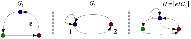
A production in essence is what we have done, with a LHS made up of labels and a graph as RHS. The notation $H=[e/G_{1}]$, also $G\Rightarrow[e/G_{1}]$, is standard to mean that graph (hypergraph) $H$ is obtained by deleting edge $e$ and plugging in graph $G_{1}$.

A hyperedge is defined in [23] (Chap. 2) as an atomic item with a label and an ordered set of tentacles. Informally, a hypergraph is a set of nodes with a collection of hyperedges such that each tentacle is attached to one node. Note that directed graphs are a special case of hypergraphs. Normally it is established that the label of a hyperedge is the number of its tentacles.

Let’s provide a formal definition of hypergraph. For a given string $w$, the length of the string is denoted by $|w|$. For a set $A$, $A^{*}$ is the set of all strings over $A$. The free symbolwise extension $f^{*}:A^{*}\rightarrow B^{*}$ of a mapping $f:A\rightarrow B$ is defined by

$$f^{*}(a_{1}\cdots a_{k})=f(a_{1})\cdots f(a_{k}),$$ (20)

$\forall k\in\mathbb{N}$ and $a_{i}\in A$, $i\in\{1,\ldots,k\}$. Let $\mathcal{C}$ be a set of labels and let $t:\mathcal{C}\rightarrow\mathbb{N}$ be a typing function. A hypergraph $H$ over $\mathcal{C}$ is the tuple

$$\left(V,E,att,lab,ext\right)$$ (21)

where $V$ is the set of nodes, $E$ the set of hyperedges, $att:E\rightarrow V^{*}$ a mapping that assigns a sequence of pairwise distinct attachment nodes $att(e)$ to each $e\in E$, $lab:E\rightarrow\mathcal{C}$ a mapping that labels each hyperedge such that $t(lab(e))=|att(e)|$ and $ext\in V^{*}$ are pairwise distinct external nodes. The type of a hyperedge is its number of tentacles and the type of a hypergraph is its number of external nodes. The set of hypergraphs will be denoted $\mathcal{H}$, or $\mathcal{H}_{C}$ if we need to explicitly refer to the set of types.

Two hypergraphs $H$ and $H^{\prime}$ are isomorphic if there exist $i=(i_{V},i_{E})$, $i_{V}:H_{V}\rightarrow H^{\prime}_{V}$ and $i_{E}:H_{E}\rightarrow H^{\prime}_{E}$ such that:

1. $i^{*}_{V}(att_{H}(e))=att_{H^{\prime}}(i_{E}(e))$.

2. $\forall e\in E_{H}$, $lab_{H}(e)=lab_{H^{\prime}}(i_{E}(e))$.

3. $i^{*}_{V}(ext_{H})=ext_{H^{\prime}}$.

As it usually happens in algebra, equality is defined up to isomorphism. If $R=\{e_{1},\ldots,e_{n}\}\subseteq E_{H}$ is the set of hyperedges to be replaced and there is a preserving type function $r:R\rightarrow\mathcal{H}$ ($\forall e\in R$, $t(r(e))=t(e)$) such that $r(e_{i})=R_{i}$, then we write it both as $H[e_{1}/R_{1},\ldots,e_{n}/R_{n}]$ or as $H[r]$.

Hyperedge replacement belongs to the gluing approaches and follows the high level scheme introduced in Sec. 1: The replacement of $R$ in $H$ according to $r$ is performed by first removing $R$ from $E_{H}$, then $\forall e\in R$ the nodes and hyperedges of $r(e)$ are disjointly added and the $i$-th external node of $r(e)$ is fused with the $i$-th attachment node of $e$.

If a hyperedge is replaced its context is not affected. Therefore, hyperedge replacement provides a context-free type of rewriting as long as no additional application conditions are employed.

There are three nice properties fulfilled by hyperedge replacement grammars that we will briefly comment and that can be compared with the problems introduced in Sec. 3, in particular problems 2, 3 and 5, 6. Let’s assume the hypothesis on hyperedges necessary so the following formulas make sense:

• Sequentialization and Parallelism: Assuming pairwise distinct hyperedges,

  $$H[e_{1}/H_{1},\ldots,e_{n}/H_{n}]=H[e_{1}/H_{1}]\cdots H[e_{n}/H_{n}].$$ (22)

• Confluence: Let $e_{1}$ and $e_{2}$ be distinct hyperedges,

  $$H[e_{1}/H_{1}][e_{2}/H_{2}]=H[e_{2}/H_{2}][e_{1}/H_{1}].$$ (23)

• Associativity:

  $$H[e_{1}/H_{1}][e_{2}/H_{2}]=H\left[e_{2}/H_{2}[e_{1}/H_{1}]\right].$$ (24)

Note however that in hyperedge replacement grammars, confluence is a consequence of the first property which holds due to disjointness of application of grammar rules.

A production $p$ over the set of non-terminals $N\subseteq\mathcal{C}$ is an ordered pair $p=(A,R)$ with $A\in N$, $R\in\mathcal{H}$ and $t(A)=t(R)$. A direct derivation is the application of a production, i.e. the replacement of a hyperedge by a hypergraph. If $H\in\mathcal{H}$, $e\in E_{H}$ and $(lab_{H}(e),R)$ is a production then $H^{\prime}=H[e/R]$ is a direct derivation and is represented by $H\Rightarrow H^{\prime}$. As always, a derivation is a sequence of direct derivations.

Formally, a hyperedge replacement grammar is a system $H\!RG=\left(N,T,P,S\right)$ where $N$ is the set of non-terminals, $T$ is the set of terminals, $P$ is the set of productions and $S\in N$ is the start symbol.

We will finish this section with a simple example that generates the string-graph language $L\left(A^{n}B^{n}\right)=\{\left(a^{n}b^{n}\right)|n\geq 1\}$. This is the graph-theoretic counterpart of the Chomsky language that consists of strings of the form $(a^{n}b^{n})$, $n\geq 1$, i.e. that has any string with an arbitrary finite number of a’s followed by the same number of b’s, e.g. $aabb$, $aaabbb$, etc.

Figure 25: String Grammar Example

A black filled circle $\bullet$ represents an external node while non-filled circles $\circ$ are internal nodes. A box represents a hyperedge with attachments with the label inscribed in the box. A 2-edge is represented by an arrow joining the first node to the second.

The grammar is defined as $A^{n}B^{n}=\left(\{S\},\{a,b\},P,S\right)$, where the set of productions $P=\{p_{1},p_{2}\}$ is depicted in Fig. 25. Production $p_{1}$ is necessary to get the graph-string $ab$ and to stop rule application. The start graph and an evolution of the grammar -- derivation $p_{1};p_{2};p_{2}$ – can be found in Fig. 26.

Figure 26: String Grammar Derivation

15 MSOL Approach

It is possible to represent graphs as logical structures, expressing their properties by logical formulas or, in other words, use logical formulas to characterize classes of graphs and to establish their properties out of their logical description. In this section we will give a brief introduction to monadic second order logics (MSOL) for graph transformation. Refer to Chap. 5 of [23] and references therein cited.

Currently it is not possible to define graph transformation in terms of automaton (recall that in language theory it is essential to have transformations that produce outputs while traversing words or trees). Quoting B. Courcelle (Chap. 5 of [23]):

The deep reason why MSOL logic is so crucial is that it replaces for graphs $(\ldots)$ the notion of a finite automaton $(\ldots)$

The key point here is that these transformations can be defined in terms of MSOL formulas (called definable transductions).

Graph operations will allow us to define context-free sets of graphs as components of least solutions to systems of equations (without using any graph rewriting rule) and recognizable sets of graphs (without using any notion of graph automaton).

Graphs and graph properties are represented using logical structures and relations. A binary relation $R\subseteq A\times B$ is a multivalued partial mapping that we will call transduction. Recall from Sec. 4 that an interpretation in logics in essence defines semantically a structure in terms of another one, for which MSOL formulas will be used.

Let $\mathcal{R}$ be a finite set of relation symbols and let $\rho(R)$ be the arity of $R\in\mathcal{R}$. An $\mathcal{R}$-structure is the tuple $S=\left(D,(R)_{R\in\mathcal{R}}\right)$ such that $D$ is the (possibly infinite) domain of $S$ and each $R$ is a $\rho(R)$-ary relation on $D$, this is, a subset of $D^{\rho(R)}$. The class of $\mathcal{R}$-structures is denoted by $ST\!R(\mathcal{R})$.

As an example of structure, for a simple digraph $G$ made up of nodes in $V$ we have the associated $\mathcal{R}$-structure $\left|G\right|_{1}=\left(V,edg\right)$, where $(x,y)\in edg$ if and only if there is an edge starting in $x$ and ending in $y$. Note that this structure represents simple digraphs.

The set of monadic second order formulas over $\mathcal{R}$ with free variables in $\mathcal{Y}$ is represented by $\textrm{MS}\left(\mathcal{R},\mathcal{Y}\right)$. As commented in Sec. 4, languages defined by MSOL formulas are regular languages.

Let $\mathcal{Q}$ and $\mathcal{R}$ be two finite ranked sets of relation symbols and $\mathcal{W}$ a finite set of set variables (the set of parameters). A $(\mathcal{R},\mathcal{Q})$-definition scheme is a tuple of formulas of the form:

$$\Delta=\left(\phi,\psi_{1},\ldots,\psi_{k},\left(\theta_{w}\right)_{w\in Q^{*}k}\right).$$ (25)

The aim of these formulas is to define a structure $T$ in $ST\!R(\mathcal{Q})$ out of a structure $S$ in $STR(\mathcal{R})$. The notation needs some comments:

• $\phi\in\textrm{MS}(\mathcal{R},\mathcal{W})$ defines the domain of the corresponding transduction, i.e. $T$ is defined if $\phi$ is true for some assignment in $\mathcal{S}$ of values assigned to the parameters.

• $\psi_{i}\in\textrm{MS}(\mathcal{R},\mathcal{W}\cup\{x_{i}\})$ defines the domain of $T$ as the disjoint union of elements in the domain of $\mathcal{S}$ that satisfy $\psi_{i}$ for the considered assignment.

• $\theta_{w}\in\textrm{MS}(\mathcal{R},\mathcal{W}\cup\{x_{1},\ldots,x_{\rho(q)}\})$ for $w=\left(q,j\right)\in\mathcal{Q}^{*}k$, where we define $\mathcal{Q}^{*}k=\left\{w\;|\;q\in\mathcal{Q},j\in[k]^{\rho(q)}\right\}$ and $[k]=\{1,\ldots k\}$, $k\in\mathbb{N}$. Formulas $\theta_{w}$ define the relation $q_{T}$.

For a more rigorous definition with some examples, please refer to [23], Chap. 5. The important fact of transductions is that they keep monadic second order properties, i.e. monadic second order properties of $\mathcal{S}$ can be expressed as monadic second order properties in $\mathcal{T}$. Furthermore, the inverse image of a MS-definable class of structures under a definable transduction is definable (not so for the image), as well as the composition and the intersection of a definable structure with the Cartesian product of two definable structures. However, there are some “negative” results apart from that of the image, e.g. the inverse of a definable transduction is not definable neither is the intersection of two definable transductions.

The theory goes far beyond, for example by defining context free sets of graphs by systems of recursive equations, generalizing in some sense the concatenation of words in string grammars. No attention will be paid to rigorous details and definitions (again, see Chap. 5 in [23]) but a simple classical example of context free grammars will be reviewed: Let $A=\{a_{1},\ldots,a_{n}\}$ be a finite alphabet, $\varepsilon$ the empty word and $A^{*}$ the set of words over $A$. Let’s consider the context-free grammar $G=\{u\rightarrow auuv,u\rightarrow avb,v\rightarrow avb,v\rightarrow ab\}$. The corresponding system of recursive equations would be:

$$S=\left\langle u=a.(u.(u.v))+a.(v.b),v=a.(v.b)+a.b\right\rangle$$

where “.” is the concatenation. It is possible, although we will not see it, to express node replacement and hyperedge replacement in terms of systems of recursive equations.

Analogously to the way in which the equational set extends context-freeness, recognizable sets extend regular languages. For example, it is possible to show that every set of finite graphs or hypergraphs defined by a formula of an appropriate monadic second order language is recognizable with respect to an appropriate set of operations (the converse also holds in many cases).

16 Relation-Algebraic Approach

We will mainly follow [52] and [36] in this section, paying special attention to the justification that the category Graph^P has pushouts, which will be used in Chap. id1 for one of the definitions of direct derivation in Matrix Graph Grammars.

We will deviate from standard relational methods notation in favor of other which is probably more immediate for mathematicians not acquainted with it and, besides, we think eases comparison with the rest of the approaches in this chapter.

A relation $r_{1}$ from $S_{1}$ to $S_{2}$ is a subset of the Cartesian product $S_{1}\times S_{2}$, denoted by $r_{1}:S_{1}\rightharpoondown S_{2}$. Its inverse $r^{-1}:S_{2}\rightharpoondown S_{1}$ is such that $(s_{2},s_{1})\in r_{1}^{-1}\Leftrightarrow(s_{1},s_{2})\in r_{1}$. If $r_{2}:S_{2}\rightharpoondown S_{3}$ is a relation, the composition $r_{2}r_{1}\equiv r_{2}\circ r_{1}:S_{1}\rightharpoondown S_{3}$ is again a relation such that

$$(s_{1},s_{3})\in r_{2}\circ r_{1}\Leftrightarrow\left[\exists s_{2}\in S_{2}\;|\;(s_{1},s_{2})\in r_{1},(s_{2},s_{3})\in S_{2}\right].$$ (26)

As relations are sets, naive set operations are available such as inclusion ($\subseteq$), intersection ($\cap$), union ($\cup$) and difference ($-$). It is possible to form the category Rel of sets and relations (the identity relation $1_{S}=S\rightharpoondown S$ is the diagonal set of $S\times S$), which besides fulfills the following properties:

• $\left(r^{-1}\right)^{-1}=r$.

• $(r_{2}\circ r_{1})^{-1}=r_{1}^{-1}\circ r_{2}^{-1}$.

• Distributive law: $r_{2}\circ\left(\bigcup_{\alpha\in A}(r_{\alpha})\right)\circ r_{1}=\bigcup_{\alpha\in A}\left(r_{2}\circ r_{\alpha}\circ r_{1}\right)$.

A relation $f:S_{1}\rightharpoondown S_{2}$ such that $f\circ f^{-1}\subseteq 1_{S_{2}}$ is called a partial function and it is represented with an arrow instead of a harpoon, $f:S_{1}\rightarrow S_{2}$. If $1_{S_{1}}\subseteq f^{-1}\circ f$ also, then it is called a total function. Note that these are the standard set-theoretic definitions of partial function and total function. The function $f$ is injective if $f^{-1}\circ f=1_{S_{1}}$ and surjective if $f\circ f^{-1}=1_{S_{2}}$.

The category of sets and partial functions is represented by Set^P. It can be proved that Set^P has small limits and colimits, so in particular it has pushouts.

For a relation $r:S\rightharpoondown T$ its domain is also a relation $d:S\rightharpoondown S$ and is given by the formula $d(r)=\left(r^{-1}\circ r\right)\cap 1_{S}$.

In order to define graph rewriting using relations we need a relational representation of graphs. A graph $\left\langle S,r\right\rangle$ is a set $S$ plus a relation $r:S\rightharpoondown S$. A partial morphism between graph $\left\langle S_{1},r_{1}\right\rangle$ and $\left\langle S_{2},r_{2}\right\rangle$, $p:S_{1}\rightarrow S_{2}$, is a partial function $p$ such that:

$$p\circ r_{1}\circ d(p)\subseteq r_{2}\circ p.$$ (27)

It is not difficult to see that the composition of two partial morphisms of graphs is again a partial morphism of graphs. It is a bit more difficult (although still easy to understand) to show that the category Graph^P of simple graphs and partial morphisms has pushouts (Theorem 3.2 in [52]). The square depicted in Fig. 27 is a pushout in Set^P if the formula for the relation $h$ is given by:

$$h=\left(m^{*}\circ r\circ m^{*{-1}}\right)\cup\left(p^{*}\circ g\circ p^{*{-1}}\right).$$ (28)

A production is defined similarly to the SPO case, as a triple of two graphs $\left\langle L,l\right\rangle$, $\left\langle R,r\right\rangle$ and a partial morphism $p:L\rightarrow R$. A match for $p$ is a morphism of graphs $M:\left\langle L,l\right\rangle\rightarrow\left\langle G,g\right\rangle$. A production plus a match is a direct derivation. As always, a derivation is a finite sequence of direct derivations.

Figure 27: Pushout for Simple Graphs (Relational) and Direct Derivation

Equation (28) defines a pushout in category Set^P which is different than a rewriting square (a direct derivation). If we want the rewriting rule to be a pushout, the relation in $\left\langle H,h\right\rangle$ must be defined by the equation:

$$h=\left(m^{*}\circ r\circ m^{*{-1}}\right)\cup\left[p^{*}\circ\left(g-m^{-1}\circ l\circ m\right)\circ p^{*{-1}}\right].$$ (29)

The relation-algebraic approach is based almost completely in relational methods. To illustrate the main differences with respect to categorical approaches an example taken from [36] follows that deals with categorical products.

Example.$\square$In order to define the categorical product – see Sec. 5 – it is necessary to check the universal property of being a terminal object, which is a global condition (it should be checked against the rest of candidate elements, in principle all elements in the category). In contrast, in relation algebras, the direct product of two objects $X$ and $Y$ is a triple $\left(P,\Pi_{X},\Pi_{Y}\right)$ satisfying the following properties:

• $\Pi_{X}\circ\Pi^{-1}_{X}=1_{X}$ and $\Pi_{Y}\circ\Pi^{-1}_{Y}=1_{Y}$.

• $\Pi_{Y}\circ\Pi_{X}^{-1}=\mathbb{U}$.

• $\left(\Pi_{X}^{-1}\circ\Pi_{X}\right)\cap\left(\Pi_{Y}^{-1}\circ\Pi_{Y}\right)=1_{P}$.

where $\mathbb{U}$ is the universal relation (to be defined below). Note that this is a local condition, in the sense that it only involves functions without quantification (in Category theory this sort of characterizations are more like for all objects in the class there exists a unique morphism such that…). $\blacksquare$

The relational approach is based on the notion of allegory which is a category $\mathcal{C}$ as defined in Sec. 5 – the underlying category – plus two operations (^-1 and $\cap$) with the following properties:

• $\left(r^{-1}\right)^{-1}=r$; $\left(r\circ s\right)^{-1}=s^{-1}\circ r^{-1}$; $\left(r_{1}\cap r_{2}\right)^{-1}=r_{1}^{-1}\cap r_{2}^{-1}$.

• $r_{1}\circ\left(r_{2}\cap r_{3}\right)\subseteq\left(r_{1}\circ r_{2}\right)\cap\left(r_{1}\circ r_{3}\right)$.

• Modal rule: $\left(r_{1}\cap r_{2}\right)\circ r_{3}\subseteq r_{1}\circ\left[r_{3}\cap\left(r_{2}\circ r_{1}^{-1}\right)\right]$.

The universal relation $\mathbb{U}$ for two objects $X$ and $Y$ in an allegory is the maximal element in the set of morphisms from $X$ to $Y$, if it exists. If there is a least element, then it is called an empty relation or a zero relation.

It is possible to obtain the other modal rule starting with the axioms of allegories:

$$\left(r_{1}\circ r_{2}\right)\circ r_{3}\subseteq\left[r_{3}\cap\left(r_{2}\circ r_{3}^{-1}\right)\right]\circ r_{2},$$ (30)

which can be synthesized in the so-called Dedekind formula:

$$\left(r_{1}\circ r_{2}\right)\circ r_{3}\subseteq\left[r_{3}\cap\left(r_{2}\circ r_{3}^{-1}\right)\right]\circ\left[r_{3}\cap\left(r_{2}\circ r_{1}^{-1}\right)\right].$$ (31)

A locally complete distributive allegory is called a Dedekind category. A distributive allegory is an allegory with joins and zero element; locally completeness refer to distributivity of composition with respect to joins.

By using Dedekind categories [36] provides a variation of the DPO approach in which graph variables and replication is possible. We will not introduce it here because it would take too long, due mainly to notation and formal definitions, and it is not used in our approach.

As a final remark, [36] proceeds by defining pushouts, pullbacks, complements and an amalgamation of pushouts and pullbacks (called pullouts) over Dedekind categories to define pullout rewriting.

17 Summary and Conclusions

The intention of this quick summary is to make an up-to-date review of the main approaches to graph grammars and graph transformation systems: Categorical, relational, set-theoretical and logical. The theory developed so far for any of these approaches goes far beyond what has been exposed here. The reader is referenced to cites spread across the chapter for further study.

Throughout the rest of the book we will see that their influence in Matrix Graph Grammars varies considerably depending on the topic. For example, our basic diagram for graph rewriting is similar to that of SPO but the way to deal with restrictions on rules (application conditions) is much more “logical”, so to speak.

We are now in the position to introduce the basics of our proposal for graph grammars. This will be carried out in the next chapter, Chap. id1, with the peculiarity that (to some extent) there is no need for a match of the rule’s left hand side, i.e. we have productions and not direct derivations. This is further studied in Chapter id1 with the notion of initial digraph and composition.

Chapter Matrix Graph Grammars Fundamentals

In this chapter and the next one, ideas outlined in Chap. id1 will be soundly based, assuming a background knowledge on the material of Secs. 4, 6 and 9. No matching to any host graph is assumed, although identification of elements (in essence, nodes) of the same type will be specified through completion.

Analysis techniques developed in this chapter include compatibility of productions and sequences as well as coherence of sequences. These concepts will be used to tackle applicability (problem 1), sequential independence (problem 3) and reachability (problem 4).

In Sec. 18 the dynamic nature of a single grammar rule is developed together with some basic facts. The operation of completion is studied in Sec. 19, which basically permits algebraic operations to be performed as one would like. Section 20 deals with sequences, i.e. ordered sets of grammar rules applied one after the other. To this end we will introduce the concept of coherence. Due to their importance, sequences will be studied in deep detail in Chap. id1.

18 Productions and Compatibility

A production (also known as grammar rule) is defined as an application which transforms a simple digraph into another simple digraph, $p:L\rightarrow R$. We can describe a production $p$ with two matrices (those with an $E$ superindex) and two vectors (those with an $N$ superindex), $p=(L^{E},R^{E},L^{N},R^{N})$, where the components are respectively the left hand side edges matrix $\left(L^{E}\right)$ and nodes vector $\left(L^{N}\right)$, and the right hand side edges matrix $\left(R^{E}\right)$ and nodes vector $\left(R^{N}\right)$.

$L^{E}$ and $R^{E}$ are the adjacency matrices and $L^{N}$ and $R^{N}$ are the nodes vector as studied in Sec. 6. A formal definition is given for further reference:

Definition 18.1 (Production - Static Formulation)

A grammar rule or production $p$ is a partial morphism between two simple digraphs $L$ and $R$, and can be specified by the tuple

$$p=\left(L^{E},R^{E},L^{N},R^{N}\right),$$ (32)

where E stands for edge and N for node. L is the left hand side and R is the right hand side.

It might seem redundant to specify nodes as they are already in the adjacency matrix. The reason is that they can be added or deleted during rewriting. Nodes and edges are considered separately, although it could be possible to synthesize them in a single structure using tensor algebra. See the construction of the incidence tensor – Def. 47.1 – in Sec. 47.

It is more interesting to characterize the dynamic behaviour of rules for which matrices will be used, describing the basic actions that can be performed by a production: Deletion and addition of nodes and edges. Our immediate target is to get a dynamic formulation.

In this book $p$ will be injective unless otherwise stated. A production models deletion and addition actions on both edges and nodes, carried out in the order just mentioned, i.e. first deletion and then addition. Appropriate matrices are introduced to represent them.

Definition 18.2 (Deletion and Addition of Edges)

Matrices for deletion and addition of edges are defined elementwise by the formulas

$$e^{E}=\left(e\right)_{ij}=\left\{\begin{array}[]{ll}1&\qquad\textrm{if edge $(i,j)$ is to be erased}\\ 0&\qquad\textrm{otherwise}\\ \end{array}\right.$$ (33)

$$r^{E}=\left(r\right)_{ij}=\left\{\begin{array}[]{ll}1&\qquad\textrm{if edge $(i,j)$ is to be added}\\ 0&\qquad\textrm{otherwise}\\ \end{array}\right.$$ (34)

For a given production $p$ as above, both matrices can be calculated through identities:

$$e^{E} \!= \!L^{E}\wedge\overline{(L^{E}\wedge R^{E})}=L^{E}\wedge\left(\overline{L^{E}}\vee\overline{R^{E}}\right)=L^{E}\wedge\overline{R^{E}}$$ (35)

$$r^{E} \!= \!R^{E}\wedge\overline{(L^{E}\wedge R^{E})}=R^{E}\wedge\left(\overline{R^{E}}\vee\overline{L^{E}}\right)=R^{E}\wedge\overline{L^{E}}$$ (36)

where $L^{E}\wedge R^{E}$ are the elements that are preserved by the rule application (similar to the $K$ component in DPO rules, see Sec. 11). Thus, using previous construction, the following two conditions hold and will be frequently used: Edges can be added if they do not currently exist and may be deleted only if they are present in the left hand side (LHS) of the production.

$$r^{E}\wedge\overline{L^{E}} = R^{E}\wedge\overline{L^{E}}\wedge\overline{L^{E}}=r^{E}$$ (37)

$$e^{E}\wedge L^{E} = L^{E}\wedge\overline{R^{E}}\wedge L^{E}=e^{E}.$$ (38)

In a similar way, vectors for the deletion and addition of nodes can be defined:

Definition 18.3 (Deletion and Addition of Nodes)

$$e^{N}=\left(e\right)_{i}=\left\{\begin{array}[]{ll}1&\qquad\textrm{if node \emph{i} is to be erased}\\ 0&\qquad\textrm{otherwise}\\ \end{array}\right.$$ (39)

$$r^{N}=\left(r\right)_{i}=\left\{\begin{array}[]{ll}1&\qquad\textrm{if node \emph{i} is to be added}\\ 0&\qquad\textrm{otherwise}\\ \end{array}\right.$$ (40)

Figure 28: Example of Production

Example.$\square$An example of production is graphically depicted in Fig. 28. Its associated matrices are:

$$L_{1}^{E}=\left[\begin{array}[]{cccc}\vskip-6.0pt0&1&1&|\;2\\ \vskip-6.0pt0&0&0&|\;4\\ \vskip-6.0pt1&0&1&|\;5\\ \end{array}\right]\;\;L_{1}^{N}=\left[\begin{array}[]{cc}\vskip-6.0pt1&|\;2\\ \vskip-6.0pt1&|\;4\\ \vskip-6.0pt1&|\;5\\ \end{array}\right]\;\;R_{1}^{E}=\left[\begin{array}[]{cccc}\vskip-6.0pt0&1&1&|\;2\\ \vskip-6.0pt0&1&0&|\;3\\ \vskip-6.0pt0&1&1&|\;5\\ \end{array}\right]\;\;R_{1}^{N}=\left[\begin{array}[]{cc}\vskip-6.0pt1&|\;2\\ \vskip-6.0pt1&|\;3\\ \vskip-6.0pt1&|\;5\\ \end{array}\right]$$

$$e_{1}^{E}=\left[\begin{array}[]{cccc}\vskip-6.0pt0&1&0&|\;2\\ \vskip-6.0pt0&0&0&|\;4\\ \vskip-6.0pt1&0&0&|\;5\\ \end{array}\right]\quad e_{1}^{N}=\left[\begin{array}[]{cc}\vskip-6.0pt0&|\;2\\ \vskip-6.0pt1&|\;4\\ \vskip-6.0pt0&|\;5\\ \end{array}\right]\quad r_{1}^{E}=\left[\begin{array}[]{cccc}\vskip-6.0pt0&1&0&|\;2\\ \vskip-6.0pt0&1&0&|\;3\\ \vskip-6.0pt0&1&0&|\;5\\ \end{array}\right]\quad r_{1}^{N}=\left[\begin{array}[]{cc}\vskip-6.0pt0&|\;2\\ \vskip-6.0pt1&|\;3\\ \vskip-6.0pt0&|\;5\\ \end{array}\right]$$

The last column of the matrices specify node ordering, which is assumed to be equal by rows and by columns. The characterization of productions through matrices will be completed by introducing the nihilation matrix (Sec. 21) and the negative initial digraph (Sec. 24). They keep track of all elements that can not be present in the graph (dangling edges and those to be added by the production). For an example of production with all its matrices, please see the one on page 19. $\blacksquare$

Now we state some basic properties that relate the adjacency matrices and $e$ and $r$.

Proposition 18.4 (Rewriting Identities)

Let $p:L\rightarrow R$ be a production. The following identities are fulfilled:

$$r^{E}\wedge\overline{e^{E}}=r^{E}\qquad r^{N}\wedge\overline{e^{N}}=r^{N}$$ (41)

$$e^{E}\wedge\overline{r^{E}}=e^{E}\qquad e^{N}\wedge\overline{r^{N}}=e^{N}$$ (42)

$$R^{E}\wedge\overline{e^{E}}=R^{E}\qquad R^{N}\wedge\overline{e^{N}}=R^{N}$$ (43)

$$L^{E}\wedge\overline{r^{E}}=L^{E}\qquad L^{N}\wedge\overline{r^{N}}=L^{N}$$ (44)

Proof
$\square$It is straightforward to prove these results using basic Boolean identities. Only the first one is included:

$$r^{E}\wedge\overline{e^{E}} = \left(\overline{L^{E}}\wedge R\right)\wedge\left(\overline{L^{E}\wedge\overline{R^{E}}}\right)=$$ (45)

$$= \left(\overline{L^{E}}\wedge R\wedge\overline{L^{E}}\right)\vee\left(\overline{L^{E}}\wedge R^{E}\wedge R^{E}\right)=$$

$$= \left(\overline{L^{E}}\wedge R^{E}\right)\vee\left(\overline{L^{E}}\wedge R^{E}\right)=r^{E}\vee r^{E}=r^{E}.$$

The rest of the identities follow easily by direct substitution of definitions. $\blacksquare$

First two equations say that edges or nodes cannot be rewritten – erased and created or vice versa – by a rule application (a consequence of the way in which matrices $e$ and $r$ are calculated). This is because, as we will see in formulas (47) and (48), elements to be deleted are those specified by $e$ and those to be added are those in $r$, so common elements are:

$$e\wedge r=e\wedge\overline{r}\wedge r\wedge\overline{e}=0.$$ (46)

This contrasts with the DPO approach, in which edges and nodes can be rewritten in a single rule. The remaining two conditions state that if a node or edge is in the right hand side (RHS), then it can not be deleted, and that if a node or edge is in the LHS, then it can not be created.

Finally we are ready to characterize a production $p:L\rightarrow R$ using deletion and addition matrices, starting from its LHS:

$$R^{N}=r^{N}\vee\left(\overline{e^{N}}\wedge L^{N}\right)$$ (47)

$$R^{E}=r^{E}\vee\left(\overline{e^{E}}\wedge L^{E}\right).$$ (48)

The resulting graph $R$ is calculated by first deleting the elements in the initial graph – $\overline{e}\wedge L$ – and then adding the new elements – $r\vee\left(\overline{e}\wedge L\right)$ –. It can be proved using Proposition 18.4 that, in fact, it doesn’t matter whether deletion is carried out first and addition afterwards or vice versa.

Remark.$\square$In the rest of the book we will omit $\wedge$ if possible, and avoid unnecessary parenthesis bearing in mind that $\wedge$ has precedence over $\vee$. So, e.g. formula (48) will be written

$$R^{E}=r^{E}\vee\overline{e^{E}}L^{E}.$$ (49)

Besides, if there is no possible confusion due to context or a formula applies to both edges and nodes, superscripts can be omitted. For example, the same formula would read $R=r\vee\overline{e}L$. $\blacksquare$

There are two ways to characterize a production so far, either using its initial and final states (see Definition 18.1) or the operations it specifies:

$$p=\left(e^{E},r^{E},e^{N},r^{N}\right).$$ (50)

As a matter of fact, they are not completely equivalent. Using $L$ and $R$ gives more information because those elements which are present in both of them are mandatory if the production is to be applied to a host graph, but they do not appear in the e-r characterization. An alternate and complete definition to (32) is

$$p=\left(L^{E},e^{E},r^{E},L^{N},e^{N},r^{N}\right).$$ (51)

A dynamic definition of grammar rule is postponed until Sec. 24, Definition 21.1 because there is a useful matrix (the nihilation matrix) that has not been introduced yet.

Some conditions have to be imposed on matrices and vectors of nodes and edges in order to keep compatibility when a rule is applied, that is, to avoid dangling edges once the rule is applied. It is not difficult to extend the definition of compatibility from adjacency matrices (see Def. 6.2) to productions:

Definition 18.5 (Compatibility)

A production $p:L\rightarrow R$ is compatible if $R=p(L)$ is a simple digraph.

From a conceptual point of view the idea is the same as that of the dangling condition in DPO. Also, what is demanded here is completeness of the underlying space $\textbf{Graph}^{\textbf{P}}$ with respect to the operations defined.

Next we enumerate the implications for Matrix Graph Grammars of compatibility. Recall that ^t denotes transposition:

1. An incoming edge cannot be added $\left(r^{E}\right)$ to a node that is going to be deleted $\left(e^{N}\right)$:

   $$\left\|r^{E}\odot e^{N}\right\|_{1}=0.$$ (52)

   Similarly, for outgoing edges $\left(r^{E}\right)^{t}$, the condition is:

   $$\left\|\left(r^{E}\right)^{t}\odot e^{N}\right\|_{1}=0.$$ (53)

2. Another forbidden situation is deleting a node with some incoming edge, if that edge is not deleted as well:

   $$\left\|\overline{e^{E}}\,L^{E}\odot e^{N}\right\|_{1}=0.$$ (54)

   Similarly for outgoing edges:

   $$\left\|\left(\overline{e^{E}}\,L^{E}\right)^{t}\odot e^{N}\right\|_{1}=0.$$ (55)

   Note that $\overline{e}^{E}L^{E}$ are elements preserved (used but not deleted) by production $p$.

3. It is not possible to add an incoming edge $\left(r^{E}\right)$ to a node which is neither present in the LHS $\left(\overline{L}^{N}\right)$ nor added $\left(\overline{r}^{N}\right)$ by the production:

   $$\left\|r^{E}\odot\left(\overline{r^{N}}\,\overline{L^{N}}\right)\right\|_{1}=0.$$ (56)

   Similarly, for edges starting in a given node:

   $$\left\|\left(r^{E}\right)^{t}\odot\left(\overline{r^{N}}\,\overline{L^{N}}\right)\right\|_{1}=0.$$ (57)

4. Finally, our last conditions state that it is not possible that an edge reaches a node which does not belong to the LHS and which is not going to be added:

   $$\left\|\left(\overline{e^{E}}L^{E}\right)\odot\left(\overline{r^{N}}\,\overline{L^{N}}\right)\right\|_{1}=0.$$ (58)

   And again, for outgoing edges:

   $$\left\|\left(\overline{e^{E}}L^{E}\right)^{t}\odot\left(\overline{r^{N}}\,\overline{L^{N}}\right)\right\|_{1}=0.$$ (59)

Thus we arrive naturally at the next proposition:

Proposition 18.6

Let $p:L\rightarrow R$ be a production. If conditions (52) – (59) are fulfilled then $R=p(L)$ is compatible.

Proof
$\square$ We have to check $\left\|\left(M_{E}\vee M_{E}^{t}\right)\odot\overline{M_{N}}\right\|_{1}=0$, with $M_{E}=r^{E}\vee\overline{e^{E}}L^{E}$ and $\overline{M}_{N}=\overline{r^{N}}\left(e^{N}\vee\overline{L^{N}}\right)$. Applying (42) in the second equality we have

$$\left(M_{E}\right. \vee \left.M_{E}^{t}\right)\odot\overline{M}_{N}=\left[\left(r^{E}\vee\overline{e^{E}}L^{E}\right)\vee\left(r^{E}\vee\overline{e^{E}}L^{E}\right)^{t}\right]\odot\left[\overline{r^{N}}\left(e^{N}\vee\overline{L^{N}}\right)\right]=$$ (60)

$$= \left[r^{E}\vee\overline{e^{E}}L^{E}\vee\left(r^{E}\right)^{t}\vee\left(\overline{e^{E}}L^{E}\right)^{t}\right]\odot\left(e^{N}\vee\overline{r^{N}}\,\overline{L^{N}}\right).$$

Synthesizing conditions (52)  – (59) or expanding eq. (60) the proof is completed. $\blacksquare$

A full example is worked out in the next section, together with further explanations on node identification across productions and types.

19 Types and Completion

Besides characterization (with compatibility), in practice we will need to endorse graphs with some “semantics” (types). These types will impose some restrictions on the way algebraic operations can be carried out (completion). This section is somewhat informal. For a more formal exposition, please refer to [67] and [66], Sec. 2.

Grammars in essence rely on the possibility to apply several morphisms (productions) in sequence, generating languages. At grammar design time we do not know in general which actual initial state is to be studied but probably we do know which elements make up the system under consideration and what properties we are going to study. For example, in a local area network we know that there are messages, clients, servers, routers, hubs, switches and cables. We also know that we are interested in dependency, deadlock and failure recovery although we probably do not know which actual net we want to study.

It seems natural to introduce types, which are simply a level of abstraction in the set of elements under consideration. For example, in previous paragraph, messages, clients, servers, etc would be types. So there is a ground level in which real things are (one actual hub) and another a little bit more abstract level in which families of elements live.

Figure 29: Examples of Types

Example.$\square$Along this book we will use two ways of typing productions. The first manner will be to use natural numbers $\mathbb{N}>0$ and primes to distinguish between elements. To the left side of Fig. 29 there is a typical simple digraph with three nodes $1$ (they are of type $1$). This is correct as long as we do not need to operate with them. During “runtime”, i.e. if some algebraic operation is to be carried out, it is mandatory to distinguish between different elements, so primes are appended as depicted to the center of the same figure.

For the second way of typing productions, check out a small network to the left of Fig. 29 where there are two clients – (1:C) and (2:C) – one switch – (1:SW) – one router – (1:R) – and one server – (1:S) –. Types are $C$, $SW$, $R$ and $S$ and instead of primes we use natural numbers to distinguish among elements of the same type.

Their adjacency matrices are:

$$\left[\begin{array}[]{ccccl}\vskip-6.0pt1&0&0&0&|\;1^{\prime}\\ \vskip-6.0pt0&0&0&0&|\;1^{\prime\prime}\\ \vskip-6.0pt0&0&1&1&|\;1^{\prime\prime\prime}\\ \vskip-6.0pt1&1&1&0&|\;2\\ \end{array}\right]\qquad\left[\begin{array}[]{cccccl}\vskip-6.0pt0&0&1&0&1&|\;1:C\\ \vskip-6.0pt0&0&0&0&1&|\;2:C\\ \vskip-6.0pt0&0&1&1&0&|\;1:R\\ \vskip-6.0pt0&0&0&0&0&|\;1:S\\ \vskip-6.0pt1&0&0&1&1&|\;1:SW\\ \end{array}\right]$$

$\blacksquare$

Nodes of the same type can be identified across productions or when performing any kind of operation, while nodes of different types must remain unrelated. A production can not change the type of any node. In some sense, nodes in the left and right hand sides of productions specify their types. Matching (refer to Chap. id1) transforms them in “actual” elements.

Types of edges are given by the type of its initial and terminal nodes. In the example of Fig. 29, the type of edge $e$ is $(1,2)$ and the type of edge $e^{\prime}$ is $(2,1)$. For edges, types $(1,2)$ and $(2,1)$ are different. See [10].

A type is just an element of a predefined set $\mathcal{T}$ and the assignment of types to nodes of a given graph $G$ is just a (possibly non-injective) total function from the graph under consideration to the set of types, $t_{G}:G\rightarrow\mathcal{T}$, such that it defines an equivalence relation $\sim$ in $G$. It is important to have disjoint types (something for granted if the relation is an equivalence relation) so one element does not have two types. In previous example, the first way of typing nodes would be $\mathcal{T}_{1}=\mathbb{N}>0$ and the second $\mathcal{T}_{2}=\left\{(\alpha:\beta)|\alpha\in\mathbb{N}>0,\beta\in\{C,S,R,SW\}\right\}$.

The notion of type is associated to the underlying algebraic structure and normally will be specified using an extra column on matrices and vectors. Conditions and restrictions on types and the way they relate to each other can be specified using restrictions (see Chap. id1).

Next we introduce the concept of completion. In previous sections we have assumed that when operating with matrices and vectors these had the same size, but in general matrices and vectors represent graphs with different sets of nodes or edges, although probably there will be common subsets.

Completion modifies matrices (and vectors) to allow some specified operation. Two problems may occur:

1. Matrices may not fully coincide with respect to the nodes under consideration.

2. Even if they are the same, they may well not be ordered as needed.

To address the first problem matrices and vectors are enlarged, adding the missing vertexes to the edge matrix and setting their values to zero. To declare that these elements do not belong to the graph under consideration, the corresponding node vector is also enlarged setting to zero the newly added vertexes.

If for example an and is specified between two matrices, say $A\wedge B$, the first thing to do is to reorder elements so it makes sense to and element by element, i.e. elements representing the same node are operated. If we are defining a grammar on a computer, the tool or environment will automatically do it but some procedure has to be followed. For the sake of an example, the following is proposed:

1. Find the set $C$ of common elements.

2. Move elements of $C$ upwards by rows in $A$ and $B$, maintaining the order. A similar operation must be done moving corresponding elements to the left by columns.

3. Sort common elements in $B$ to obtain the same ordering as in $A$.

4. Add remaining elements in $A$ to $B$ sorted as in $A$, immediately after the elements accessed in previous step.

5. Add remaining elements in $B$ to $A$ sorted as in $B$.

Addition of elements and reordering (the operations needed for completion) extend and modify productions syntactically but not from a semantical point of view.

Figure 30: Example of Production (Rep.)

Example.$\square$Consider the production depicted in Fig. 30. Its associated matrices are represented below. As already commented above, the notation for matrices will be extended a little bit in order to specify node and edges types. It is assumed for the adjacency matrix that it is equally ordered by rows so we do not add any row. If it is clear from context or there is a problem with space, this labeling column will not appear, making it explicit in words if needed.

$$L_{1}^{E}=\left[\begin{array}[]{cccc}\vskip-6.0pt0&1&1&|\;2\\ \vskip-6.0pt0&0&0&|\;4\\ \vskip-6.0pt1&0&1&|\;5\\ \end{array}\right]\;\;L_{1}^{N}=\left[\begin{array}[]{cc}\vskip-6.0pt1&|\;2\\ \vskip-6.0pt1&|\;4\\ \vskip-6.0pt1&|\;5\\ \end{array}\right]\;\;R_{1}^{E}=\left[\begin{array}[]{cccc}\vskip-6.0pt0&1&1&|\;2\\ \vskip-6.0pt0&1&0&|\;3\\ \vskip-6.0pt0&1&1&|\;5\\ \end{array}\right]\;\;R_{1}^{N}=\left[\begin{array}[]{cc}\vskip-6.0pt1&|\;2\\ \vskip-6.0pt1&|\;3\\ \vskip-6.0pt1&|\;5\\ \end{array}\right]$$

$$e_{1}^{E}=\left[\begin{array}[]{cccc}\vskip-6.0pt0&1&0&|\;2\\ \vskip-6.0pt0&0&0&|\;4\\ \vskip-6.0pt1&0&0&|\;5\\ \end{array}\right]\quad e_{1}^{N}=\left[\begin{array}[]{cc}\vskip-6.0pt0&|\;2\\ \vskip-6.0pt1&|\;4\\ \vskip-6.0pt0&|\;5\\ \end{array}\right]\quad r_{1}^{E}=\left[\begin{array}[]{cccc}\vskip-6.0pt0&1&0&|\;2\\ \vskip-6.0pt0&1&0&|\;3\\ \vskip-6.0pt0&1&0&|\;5\\ \end{array}\right]\quad r_{1}^{N}=\left[\begin{array}[]{cc}\vskip-6.0pt0&|\;2\\ \vskip-6.0pt1&|\;3\\ \vskip-6.0pt0&|\;5\\ \end{array}\right]$$

For example, if the operation $\overline{e_{1}^{E}}\,r_{1}^{E}$ was to be performed, then both matrices must be completed. Following the steps described above we obtain:

$$e_{1}^{E}=\left[\begin{array}[]{ccccc}\vskip-6.0pt0&1&0&0&|\;2\\ \vskip-6.0pt0&0&0&0&|\;4\\ \vskip-6.0pt1&0&0&0&|\;5\\ \vskip-6.0pt0&0&0&0&|\;3\\ \end{array}\right]\,r_{1}^{E}=\left[\begin{array}[]{ccccc}\vskip-6.0pt0&0&0&1&|\;2\\ \vskip-6.0pt0&0&0&0&|\;4\\ \vskip-6.0pt0&0&0&1&|\;5\\ \vskip-6.0pt0&0&0&1&|\;3\\ \end{array}\right]\,L_{1}^{N}=\left[\begin{array}[]{cc}\vskip-6.0pt1&|\;2\\ \vskip-6.0pt1&|\;4\\ \vskip-6.0pt1&|\;5\\ \vskip-6.0pt0&|\;3\\ \end{array}\right]\,R_{1}^{N}=\left[\begin{array}[]{cc}\vskip-6.0pt1&|\;2\\ \vskip-6.0pt0&|\;4\\ \vskip-6.0pt1&|\;5\\ \vskip-6.0pt1&|\;3\\ \end{array}\right]$$

where, besides the erasing and addition matrices, the completion of the nodes vectors for both left and right hand sides are displayed.

Now we check whether $r^{N}_{1}\vee\overline{e^{N}_{1}}\,L^{N}_{1}$ and $r^{E}_{1}\vee\overline{e^{E}_{1}}\,L^{E}_{1}$ are compatible, i.e. $R^{E}_{1}$ and $R^{N}_{1}$ define a simple digraph. Proposition 6.4 and equation (4) are used, so we need to compute eq. (60) and, as

$$r^{E}_{1}\vee\overline{e^{E}_{1}}L^{E}_{1}=\left[\begin{array}[]{ccccc}\vskip-6.0pt0&0&1&1&|\;2\\ \vskip-6.0pt0&0&0&0&|\;4\\ \vskip-6.0pt0&0&1&1&|\;5\\ \vskip-6.0pt0&0&0&1&|\;3\\ \end{array}\right]\qquad\overline{r^{N}_{1}}\left(e^{N}_{1}\vee\overline{L^{N}_{1}}\right)=\left[\begin{array}[]{cc}\vskip-6.0pt0&|\;2\\ \vskip-6.0pt1&|\;4\\ \vskip-6.0pt0&|\;5\\ \vskip-6.0pt0&|\;3\\ \end{array}\right]$$

substituting we finally arrive at

$$(\ref{eq:OneProdCompatibility})=\left(\left[\begin{array}[]{ccccc}\vskip-6.0pt0&0&1&1&|\;2\\ \vskip-6.0pt0&0&0&0&|\;4\\ \vskip-6.0pt0&0&1&1&|\;5\\ \vskip-6.0pt0&0&0&1&|\;3\\ \end{array}\right]\vee\left[\begin{array}[]{ccccc}\vskip-6.0pt0&0&0&0&|\;2\\ \vskip-6.0pt0&0&0&0&|\;4\\ \vskip-6.0pt1&0&1&0&|\;5\\ \vskip-6.0pt1&0&1&1&|\;3\\ \end{array}\right]\right)\odot\left[\begin{array}[]{cc}\vskip-6.0pt0&|\;2\\ \vskip-6.0pt1&|\;4\\ \vskip-6.0pt0&|\;5\\ \vskip-6.0pt0&|\;3\\ \end{array}\right]=\left[\begin{array}[]{cc}\vskip-6.0pt0&|\;2\\ \vskip-6.0pt0&|\;4\\ \vskip-6.0pt0&|\;5\\ \vskip-6.0pt0&|\;3\\ \end{array}\right]$$

as desired. $\blacksquare$

It is not possible, once the process of completion has finished, to have two nodes with the same number inside the same production because from an operational point of view it is mandatory to know all relations between nodes. If completion is applied to a sequence then we will speak of a completed sequence.

Note that up to this point only the production itself has been taken into account, with no reference to the state of the system (host graph). Although this is half truth – as you will promptly see – we may say that we are starting the analysis of grammar rules without the need of any matching, i.e. we will analyze productions and not necessarily direct derivations, with the advantage of gathering information at a grammar definition stage. Of course this is a desirable property as long as results of this analysis can be used for derivations (during runtime).

In some sense completion and matching are complementary operations: Inside a sequence of productions, matchings – as side effect – differentiate or relate nodes (and hence, edges) of productions. Completion imposes some restrictions to possible matchings. If we have the image of the evolution of a system by the application of a derivation as depicted in Fig. 37 on p. 37, then matchings can be viewed as vertical identifications, while completions can be seen as horizontal identifications.

The way completion has been introduced, there is a deterministic part limited to adding dummy elements and a non-deterministic one deciding on identifications. It should be possible to define it as an operator whose output would be all possible relations among elements (of the same type), i.e. completion of two matrices would not be two matrices anymore, but the set of matrices in which all possible combinations would be considered (or a subset if some of them can be discarded). This is related to the definition of initial digraph set in Sec. 29 and the structure therein studied.

20 Sequences and Coherence

Once we are able to characterize a single production, we can proceed with the study of finite collections of them. Two main operations, composition and concatenation, which are in fact closely related, are introduced in this and next sections, along with notions that make it possible to speak of “potential definability”: Coherence and compatibility.

In order to ease exposition, in this section we shall prove partial results concerning coherence: we shall consider productions that do not generate dangling edges. Coherence characterization taking into account dangling edges can be found in Sec. 21 or somewhat generalized in [66].

Definition 20.1 (Concatenation)

Let $\mathfrak{G}$ be a grammar. Given a collection of productions $\{p_{1},\ldots,p_{n}\}\subset\mathfrak{G}$, the notation $s_{n}=p_{n};p_{n-1};\ldots;p_{1}$ defines a sequence (concatenation) of productions establishing an order in their application, starting with $p_{1}$ and ending with $p_{n}$.

Remark.$\square$In the literature of graph transformation, the concatenation operator is defined back to front, this is, in the sequence $p_{2};p_{1}$, production $p_{2}$ would be applied first and $p_{1}$ right afterwards [11]. The ordering already introduced is preferred because it follows the mathematical way in which composition is defined and represented. This issue will be raised again in Sec. 45. $\blacksquare$

It is worth stressing that there exists a total order in a sequence, one production being applied after the previous has finished, and thus intermediate states are generated. These intermediate states are indeed the difference between concatenation and composition of productions (see Sec. 25). The study of concatenation is related to the interleaving approach to concurrency, while composition is related to the explicit parallelism approach (see Sec. 11).

A production is moved forward, moved to the front or advanced if it is shifted one or more positions to the right inside a sequence of productions, either in a composition or a concatenation (it is to be applied earlier), e.g. $p_{4};p_{3};p_{2};p_{1}\mapsto p_{3};p_{2};p_{1};p_{4}$. On the contrary, move backwards or delay means shifting the production to the left, which implies delaying its application, e.g. $p_{4};p_{3};p_{2};p_{1}\mapsto p_{1};p_{4};p_{3};p_{2}$.

Definition 20.2 (Coherence)

Given the set of productions $\{p_{1},\ldots,p_{n}\}$, the completed sequence $s_{n}=p_{n};p_{n-1};\ldots;p_{1}$ is called coherent if actions of any production do not prevent actions of the productions that follow it, taking into account the effects of intermediate productions.

Coherence is a concept that deals with potential applicability to a host graph of a sequence $s_{n}$ of productions. It does not guarantee that the application of $s_{n}$ and a coherent reordering of $s_{n}$, $\sigma\left(s_{n}\right)$, lead to the same result. This latter case is a sort of generalization of sequential independence applied to sequences, which will be studied in Chap. id1.

Figure 31: Productions $q_{1}$, $q_{2}$ and $q_{3}$

Example.$\square$We extend previous example (see Fig. 30 on p. 30) with two more productions. Recall that our first production $q_{1}$ deletes edge $(5,2)$, which starts in vertex 5 and ends in vertex 2. As depicted in Fig. 31, production $q_{2}$ adds this edge and $q_{3}$ preserves it ($q_{3}$ used but does not delete this edge). Sequence $s_{3}=q_{3};q_{2};q_{1}$ would be coherent if only this vertex was considered. $\blacksquare$

Now we study the conditions that have to be satisfied by the matrices associated with a coherent and dangling-free sequence of productions. Instead of stating a result concerning conditions on coherence and proving it immediately afterwards, we begin by discussing the case of two productions in full detail, we continue with three and we finally set a theorem – Theorem 20.5 – for a finite number of them.

Let us consider the concatenation $s_{2}=p_{2};p_{1}$. In order to decide whether the application of $p_{1}$ does not exclude $p_{2}$, we impose three conditions on edges:

1. The first production – $p_{1}$ – does not delete any edge ($e^{E}_{1}$) used by the second production ($L^{E}_{2}$):

   $$e^{E}_{1}L^{E}_{2}=0.$$ (61)

2. $p_{2}$ does not add ($r^{E}_{2}$) any edge preserved (used but not deleted, $\overline{e^{E}_{1}}L^{E}_{1}$) by $p_{1}$:

   $$r^{E}_{2}L^{E}_{1}\overline{e^{E}_{1}}=0.$$ (62)

3. No common edges are added by both productions:

   $$r^{E}_{1}r^{E}_{2}=0.$$ (63)

The first condition is needed because if $p_{1}$ deletes an edge used by $p_{2}$, then $p_{2}$ would not be applicable. The last two conditions are mandatory in order to obtain a simple digraph (with at most one edge in each direction between two nodes).

Conditions (62) and (63) are equivalent to $r^{E}_{2}R^{E}_{1}=0$ because, as both are equal to zero, we can do

$0=r^{E}_{2}L^{E}_{1}\overline{e^{E}_{1}}\vee r^{E}_{2}r^{E}_{1}=r^{E}_{2}\left(r^{E}_{1}\vee\overline{e^{E}_{1}}L^{E}_{1}\right)=r^{E}_{2}R^{E}_{1}$

which may be read “$p_{2}$ does not add any edge that comes out from $p_{1}$’s application”. All conditions can be synthesized in the following identity:

$$r^{E}_{2}R^{E}_{1}\vee e^{E}_{1}L^{E}_{2}=0.$$ (64)

Our immediate target is to obtain a closed formula to represent these conditions for the case of an arbitrary finite number of productions. Applying (41) and (42), equation (64) can be transformed to get:

$$R^{E}_{1}\overline{e^{E}_{2}}r^{E}_{2}\vee L^{E}_{2}e^{E}_{1}\,\overline{r^{E}_{1}}=0.$$ (65)

A similar reasoning gives the corresponding formula for nodes:

$$R^{N}_{1}\overline{e^{N}_{2}}r^{N}_{2}\vee L^{N}_{2}e^{N}_{1}\,\overline{r^{N}_{1}}=0.$$ (66)

Remark.$\square$Note that conditions (62) and (63) do not really apply to nodes as apply to edges. For example, if a node of type 1 is to be added and nodes 1 and $1^{\prime}$ have already been appended, then by completion node $1^{\prime\prime}$ would be added. It is not possible to add a node that already exists.

However, coherence looks for conditions that guarantee that the operations specified by the productions of a sequence do not interfere one with each other. Suppose the same example but this time, for some unknown reason, the node to be added is completed as $1^{\prime}$ – this one has just been added –. If conditions of the kind of (62) and (63) are removed, then we would not detect that there is a potential problem if this sequence is applied. $\blacksquare$

Next we introduce a graphical notation for Boolean equations: A vertical arrow means and while a fork stands for or. We use these diagrams because formulas grow very fast with the number of nodes. As an example, the representation of equations (65) and (66) is shown in Fig. 32.

Figure 32: Coherence for Two Productions

Lemma 20.3

Let $s_{2}=p_{2};p_{1}$ be a sequence of productions without dangling edges. If equations  (65) and (66) hold, then $s_{2}$ is coherent.

Proof
$\square$Only edges are considered because a symmetrical reasoning sets the result for nodes. Call D the action of deleting an edge, A its addition and P its preservation, i.e. the edge appears in both LHS and RHS. Table 1 comprises all nine possibilities for two productions.

$D_{2};D_{1}$	(61)	$D_{2};P_{1}$	$\surd$	$D_{2};A_{1}$	$\surd$
$P_{2};D_{1}$	(61)	$P_{2};P_{1}$	$\surd$	$P_{2};A_{1}$	$\surd$
$A_{2};D_{1}$	$\surd$	$A_{2};P_{1}$	(62)	$A_{2};A_{1}$	(63)

Table 1: Possible Actions for Two Productions

A tick means that the action is allowed, while a number refers to the condition that prohibits the action. For example, $P_{2};D_{1}$ means that first production $p_{1}$ deletes the edge and second $p_{2}$ preserves it (in this order). If the table is looked up we find that this is forbidden by equation (61). $\blacksquare$

Now we proceed with three productions. We must check that $p_{2}$ does not disturb $p_{3}$ and that $p_{1}$ does not prevent the application of $p_{2}$. Notice that both of them are covered in our previous explanation (in the two productions case), and thus we just need to ensure that $p_{1}$ does not exclude $p_{3}$, taking into account that $p_{2}$ is applied in between:

1. $p_{1}$ does not delete ($e^{E}_{1}$) any edge used ($L^{E}_{3}$) by $p_{3}$ and not added ($\overline{r^{E}_{2}}$) by $p_{2}$:

   $$e^{E}_{1}L^{E}_{3}\overline{r^{E}_{2}}=0.$$ (67)

2. Production $p_{3}$ does not add – $r^{E}_{3}$ – any edge stemming from $p_{1}$ – $R^{E}_{1}$ – and not deleted by $p_{2}$ – $e^{E}_{2}$ –:

   $$r^{E}_{3}R^{E}_{1}\overline{e^{E}_{2}}=0.$$ (68)

Again, the last condition is needed in order to obtain a simple digraph. Performing similar manipulations to those carried out for $s_{2}$ we get the full condition for $s_{3}$, given by the equation:

$$L^{E}_{2}e^{E}_{1}\vee L^{E}_{3}\left(e^{E}_{1}\,\overline{r^{E}_{2}}\vee e^{E}_{2}\right)\vee R^{E}_{1}\left(\overline{e^{E}_{2}}r^{E}_{3}\vee r^{E}_{2}\right)\vee R^{E}_{2}r^{E}_{3}=0.$$ (69)

Proceeding as before, identity (69) is completed:

$$L^{E}_{2}e^{E}_{1}\,\overline{r^{E}_{1}} \vee L^{E}_{3}\overline{r^{E}_{2}}\left(e^{E}_{1}\,\overline{r^{E}_{1}}\vee e^{E}_{2}\right)\vee$$ (70)

$$\vee R^{E}_{1}\overline{e^{E}_{2}}\left(r^{E}_{2}\vee\overline{e^{E}_{3}}r^{E}_{3}\right)\vee R^{E}_{2}\overline{e^{E}_{3}}r^{E}_{3}=0.$$

Its representation is shown in Fig. 33 for both nodes and edges.

Figure 33: Coherence Conditions for Three Productions

Lemma 20.3 can be extended slightly to include three productions in an obvious way, but we will not discuss this further because the generalization to cover n productions is Theorem 20.5.

Example.$\square$Recall productions $q_{1}$, $q_{2}$ and $q_{3}$ introduced in Figs. 30 and 31 (on pp. 30 and 31, respectively). Sequences $q_{3};q_{2};q_{1}$ and $q_{1};q_{3};q_{2}$ are coherent, while $q_{3};q_{1};q_{2}$ is not. The latter is due to the fact that edge $(5,5)$ is deleted (D) by $q_{2}$, used (U) by $q_{1}$ and added (A) by $q_{3}$, being two pairs of forbidden actions. For the former sequences we have to check all actions performed on all edges and nodes by the productions in the order specified by the concatenation, verifying that they do not exclude each other. $\blacksquare$

Definition 20.4

Let $F(x,y)$ and $G(x,y)$ be two Boolean functions dependent on parameters $x,y\in I$ in some index set $I$. Operators delta $\bigtriangleup$ and nabla $\bigtriangledown$ are defined through the equations:

$$\bigtriangleup_{t_{0}}^{t_{1}}\left(F(x,y)\right)=\bigvee_{y=t_{0}}^{t_{1}}\left(\bigwedge_{x=y}^{t_{1}}\left(F(x,y)\right)\right)$$ (71)

$$\bigtriangledown_{t_{0}}^{t_{1}}\left(G(x,y)\right)=\bigvee_{y=t_{0}}^{t_{1}}\left(\bigwedge_{x=t_{0}}^{y}\left(G(x,y)\right)\right).$$ (72)

These operators will be useful for the general case of $n$ productions with coherence, initial digraphs, G-congruence and other concepts. A simple interpretation for both operators will be given at the end of the section.

Example.$\square$Let $F(x,y)=G(x,y)=\overline{r}_{x}e_{y}$, then we have:

$$\bigtriangleup_{1}^{3}\left(\overline{r}_{x}e_{y}\right) = \bigvee_{y=1}^{3}\left(\bigwedge_{x=y}^{3}\left(\overline{r}_{x}e_{y}\right)\right)=\overline{r}_{3}e_{3}\vee\overline{r}_{3}\overline{r}_{2}e_{2}\vee\overline{r}_{3}\overline{r}_{2}\overline{r}_{1}e_{1}=e_{3}\vee\overline{r}_{3}e_{2}\vee\overline{r}_{3}\overline{r}_{2}e_{1}.$$

$$\bigtriangledown_{3}^{5}\left(\overline{r}_{x}e_{y}\right) = \bigvee_{y=3}^{5}\left(\bigwedge_{x=3}^{x=y}\left(\overline{r}_{x}e_{y}\right)\right)=\overline{r}_{3}e_{3}\vee\overline{r}_{3}\overline{r}_{4}e_{4}\vee\overline{r}_{3}\overline{r}_{4}\overline{r}_{5}e_{5}=e_{3}\vee\overline{r}_{3}e_{4}\vee\overline{r}_{3}\overline{r}_{4}e_{5}.$$

Expressions have been simplified applying Proposition 18.4. $\blacksquare$

Now we are ready to characterize coherent sequences of arbitrary finite length.

Theorem 20.5

The dangling-free concatenation $s_{n}=p_{n};p_{n-1};\ldots;p_{2};p_{1}$ is coherent if for edges and nodes we have:

$$\bigvee_{i=1}^{n}\left(R^{E}_{i}\bigtriangledown_{i+1}^{n}\left(\overline{e^{E}_{x}}\,r^{E}_{y}\right)\vee L^{E}_{i}\bigtriangleup_{1}^{i-1}\left(e^{E}_{y}\,\overline{r^{E}_{x}}\right)\right)=0$$ (73)

$$\bigvee_{i=1}^{n}\left(R^{N}_{i}\bigtriangledown_{i+1}^{n}\left(\overline{e^{N}_{x}}\,r^{N}_{y}\right)\vee L^{N}_{i}\bigtriangleup_{1}^{i-1}\left(e^{N}_{y}\,\overline{r^{N}_{x}}\right)\right)=0.$$ (74)

Proof
$\square$Induction on the number of productions (see cases $s_{2}$ and $s_{3}$ studied above). $\blacksquare$

Figure 34: Coherence. Four and Five Productions

Figure 34 includes the graph representation of the formulas for coherence for $s_{4}=p_{4};p_{3};p_{2};p_{1}$ and $s_{5}=p_{5};p_{4};p_{3};p_{2};p_{1}$.

Example.$\square$We are going to verify that $s_{1}=q_{1};q_{3};q_{2}$ is coherent (only for edges), where $q_{i}$ are the productions introduced in previous examples. Productions are drawn again in Fig. 35 for the reader convenience. We start expanding formula (73) for $n=3$:

$$\bigvee_{i=1}^{3}\left(\right. \!\!R^{E}_{i} \!\!\left.\bigtriangledown_{i+1}^{3}\left(\overline{e^{E}_{x}}\,r^{E}_{y}\right)\vee L^{E}_{i}\bigtriangleup_{1}^{i-1}\left(e^{E}_{y}\,\overline{r^{E}_{x}}\right)\right)=R^{E}_{1}\left(\overline{e^{E}_{2}}\,r^{E}_{2}\vee\overline{e^{E}_{2}}\,\overline{e^{E}_{3}}\,r^{E}_{3}\right)\vee$$

$$\!\!\vee \!\!\!R^{E}_{2}\overline{e^{E}_{3}}r^{E}_{3}\vee L^{E}_{2}\overline{r^{E}_{1}}\,e^{E}_{1}\vee L^{E}_{3}\left(\overline{r^{E}_{1}}\,\overline{r^{E}_{2}}\,e^{E}_{1}\vee\overline{r^{E}_{2}}\,e^{E}_{2}\right)=$$

$$\!\!= \!\!\!R^{E}_{1}\left(r^{E}_{2}\vee\overline{e^{E}_{2}}\,r^{E}_{3}\right)\vee R^{E}_{2}r^{E}_{3}\vee L^{E}_{2}e^{E}_{1}\vee L^{E}_{3}\left(e^{E}_{1}\,\overline{r^{E}_{2}}\vee e^{E}_{2}\right).$$

which should be zero.

Figure 35: Productions $q_{1}$, $q_{2}$ and $q_{3}$ (Rep.)

Note that this equation applies to concatenation $s=q_{3};q_{2};q_{1}$ and thus we have to map $(1,2,3)\mapsto(2,3,1)$ to obtain

$$\underbrace{R^{E}_{2}\left(r^{E}_{3}\vee\overline{e^{E}_{3}}\,r^{E}_{1}\right)}_{(*)}\vee\underbrace{R^{E}_{3}r^{E}_{1}\vee L^{E}_{3}e^{E}_{2}}_{(**)}\vee\underbrace{L^{E}_{1}\left(e^{E}_{2}\,\overline{r^{E}_{3}}\vee e^{E}_{3}\right)}_{(***)}=0.$$ (75)

Before checking whether these expressions are zero or not, we have to complete the involved matrices. All calculations have been divided into three steps and, as they are operated with or, the result will not be null if one fails to be zero.

Only the second term (**) is expanded, with ordering of nodes not specified for a matter of space. Nodes are sorted $[2\;3\;5\;1\;4]$ both by columns and by rows, meaning for example that element $(3,4)$ is an edge starting in node 5 and ending in node 1.

$$\left[\begin{array}[]{ccccc}\vskip-6.0pt1&0&0&1&0\\ \vskip-6.0pt0&0&0&0&0\\ \vskip-6.0pt1&0&1&0&0\\ \vskip-6.0pt0&0&1&0&0\\ \vskip-6.0pt0&0&0&0&0\\ \end{array}\right]\left[\begin{array}[]{ccccc}\vskip-6.0pt0&1&0&0&0\\ \vskip-6.0pt0&1&0&0&0\\ \vskip-6.0pt0&1&0&0&0\\ \vskip-6.0pt0&0&0&0&0\\ \vskip-6.0pt0&0&0&0&0\\ \end{array}\right]\vee\left[\begin{array}[]{ccccc}\vskip-6.0pt0&0&0&1&0\\ \vskip-6.0pt1&0&0&0&0\\ \vskip-6.0pt1&0&0&0&0\\ \vskip-6.0pt0&0&0&1&0\\ \vskip-6.0pt0&0&0&0&0\\ \end{array}\right]\left[\begin{array}[]{ccccc}\vskip-6.0pt0&1&0&0&0\\ \vskip-6.0pt0&0&0&0&0\\ \vskip-6.0pt0&0&1&0&0\\ \vskip-6.0pt0&0&0&0&0\\ \vskip-6.0pt0&0&0&0&0\\ \end{array}\right]=0,$$

so the sequence is coherent where, as usual, a matrix filled up with zeros is represented by $0$.

Now consider sequence $s^{\prime}_{3}=q_{2};q_{3};q_{1}$ where $q_{2}$ and $q_{3}$ have been swapped with respect to $s_{3}$. The condition for its coherence is:

$$\underbrace{R^{E}_{1}\left(r^{E}_{3}\vee\overline{e^{E}_{3}}\,r^{E}_{2}\right)}_{(*)}\vee\underbrace{R^{E}_{3}r^{E}_{2}\vee L^{E}_{3}e^{E}_{1}}_{(**)}\vee\underbrace{L^{E}_{2}\left(e^{E}_{1}\,\overline{r^{E}_{3}}\vee e^{E}_{3}\right)}_{(***)}=0.$$ (76)

If we focus just on the first term (*) in equation (76)

$$\left[\begin{array}[]{ccccc}\vskip-6.0pt0&1&1&0&0\\ \vskip-6.0pt0&1&0&0&0\\ \vskip-6.0pt0&1&1&0&0\\ \vskip-6.0pt0&0&0&0&0\\ \vskip-6.0pt0&0&0&0&0\\ \end{array}\right]\left(\left[\begin{array}[]{ccccc}\vskip-6.0pt1&0&0&0&0\\ \vskip-6.0pt0&0&0&0&0\\ \vskip-6.0pt0&0&1&0&0\\ \vskip-6.0pt0&0&1&0&0\\ \vskip-6.0pt0&0&0&0&0\\ \end{array}\right]\vee\left[\begin{array}[]{ccccc}\vskip-6.0pt1&1&1&1&1\\ \vskip-6.0pt0&1&1&1&1\\ \vskip-6.0pt1&1&1&1&1\\ \vskip-6.0pt1&1&1&0&1\\ \vskip-6.0pt1&1&1&1&1\\ \end{array}\right]\left[\begin{array}[]{ccccc}\vskip-6.0pt0&0&0&0&1\\ \vskip-6.0pt1&0&0&0&0\\ \vskip-6.0pt1&0&0&0&0\\ \vskip-6.0pt0&0&0&0&0\\ \vskip-6.0pt0&0&0&0&0\\ \end{array}\right]\right)$$

we obtain a matrix filled up with zeros except in position (3,3) which corresponds to an edge that starts and ends in node $5$. Ordering of nodes has been omitted again due to lack of space, but it is the same as above: $[2\;3\;5\;1\;4]$.

We do not only realize that the sequence is not coherent, but in addition information on which node or edge may present problems when applied to an actual host graph is provided. $\blacksquare$

Note that a sequence not being coherent does not necessarily mean that the grammar is not well defined, but that we have to be especially careful when applying it to a host graph because it is mandatory for the match to identify all problematic parts in different places.

This information could be used when actually finding the match; a possible strategy, if parallel matching for different productions is required, is to start with those elements which may present a problem.

This section ends providing a simple interpretation of $\nabla$ and $\bigtriangleup$, which in essence are a generalization of the structure of a sequence of productions. A sequence $p_{2};p_{1}$ is a complex operation: To some potential digraph, one should start by deleting elements specified by $e_{1}$, then add elements in $r_{1}$, afterwards delete elements in $e_{2}$ and finally add elements in $r_{2}$. Generalization means that this same structure can be applied but not limited to matrices $e$ and $r$, i.e. there is an alternate sequence of “delete” and “add” operations with general expressions rather than just matrices $e$ and $r$. For example, $\nabla_{1}^{3}\left(\overline{e_{x}}R_{x}\vee L_{y}\vee r_{y}\right)$.

Operators $\nabla$ and $\bigtriangleup$ represent ascending and descending sequences. For example, $\nabla_{1}^{3}\overline{e_{x}}r_{y}=p_{1}p_{2}(r_{3})$ and $\bigtriangleup_{1}^{3}\overline{e_{x}}r_{y}=p_{3}p_{2}(r_{1})$. In some detail:

$$\nabla_{1}^{3}\overline{e}_{x}\,r_{y} = \overline{e}_{1}r_{1}\vee\overline{e}_{1}\,\overline{e}_{2}\,r_{2}\vee\overline{e}_{1}\,\overline{e}_{2}\,\overline{e}_{3}\,r_{3}=$$

$$= r_{1}\vee\overline{e}_{1}r_{2}\vee\overline{e}_{1}\,\overline{e}_{2}r_{3}=r_{1}\vee\overline{e}_{1}\left(r_{2}\vee\overline{e}_{2}r_{3}\right)=p_{1}\left(p_{2}\left(r_{3}\right)\right).$$

We will make good use of this interpretation in Chap. id1 to establish the equivalence between coherence plus compatibility of a derivation and finding its minimal and negative initial digraphs in the host graph and its negation, respectively.

As commented above, we shall return to coherence in Sec. 21, which is further generalized in [66] through so-called Boolean complexes.

21 Coherence Revisited

In this section we shall extend the results of Sec. 20 taking into account potential dangling edges. To this end we need to introduce the nihil matrix $K$, which will be very useful in the rest of the book.

Our plan now is to first make explicit all elements that should not be present in a potential match of the left hand side of a rule in a host graph, and then characterize them for a finite sequence. This is carried out defining something similar to the minimal initial digraph, the negative initial digraph. In order to keep our philosophy of making our analysis as general as possible (independent of any concrete host graph) only the elements appearing on the LHS of the productions that make up the sequence plus their actions will be taken into account.

We will refer to elements that should not be present as forbidden elements. There are two sets of elements that for different reasons should not appear in a potential initial digraph:

1. Edges added by the production, as we are limited for now to simple digraphs.

2. Edges incident to some node deleted by the production (dangling edges).

To consider elements just described, the notation to represent productions is extended with a new graph $K$ that we will call the nihilation matrix. Note that the concept of grammar rule remains unaltered because we are just making explicit some implicit information.

To further justify the naturalness of this matrix let’s oppose its meaning to that of the LHS and its interpretation as a positive application condition (the LHS must exist in the host graph in order to apply the grammar rule). In effect, $K$ can be seen as a negative application condition: If it is found in the host graph then the production can not be applied. We will dedicate a whole chapter (Chap. id1) to develop these ideas.

The order in which matrices are derived is enlarged to cope with the nihilation matrix $K$:

$$\left(L,R\right)\longmapsto\left(e,r\right)\longmapsto K.$$ (77)

Otherwise stated, a production is statically determined by its left and right hand sides $p=\left(L,R\right)$, from which it is possible to give a dynamic definition $p=\left(L,e,r\right)$, to end up with a full specification including its environmental behaviour $p=\left(L,K,e,r\right)$.

Definition 21.1 (Production - Dynamic Formulation)

A production $p$ is a morphism between two simple digraphs $L$ and $R$, and can be specified by the tuple

$$p=\left(L^{E},K^{E},e^{E},r^{E},L^{N},K^{N},e^{N},r^{N}\right).$$ (78)

Compare with Dfinition 18.1, the static formulation of production. As commented earlier in the book, it should be possible to consider nodes and edges together using the tensorial construction of Chap. id1.

Next lemma shows how to calculate $K$ using the production $p$, by applying it to a certain matrix:

Lemma 21.2 (Nihilation matrix)

Using tensor notation (see Sec. 7) let’s define $D=\overline{e^{N}}\otimes\overline{\left(e^{N}\right)}^{\,t}$, where $t$ denotes transposition. Then,

$$K^{E}=p\left(\overline{D}\right).$$ (79)

Proof
$\square$The following matrix specifies potential dangling edges incident to nodes appearing in the left hand side of $p$:

$$\overline{D}=d^{i}_{\!j}=\left\{\begin{array}[]{ll}1&\qquad if\;\left(e^{i}\right)^{N}=1\;or\;\left(e_{j}\right)^{N}=1.\\ 0&\qquad otherwise.\end{array}\right.$$ (80)

Note that $D=\overline{e^{N}}\otimes\overline{\left(e^{N}\right)}^{\,t}$. Every element incident to a node that is going to be deleted becomes dangling except edges deleted by the production. In addition, edges added by the rule can not be present, thus we have $K^{E}=r^{E}\vee\overline{e^{E}}\left(\overline{D}\right)=p\left(\overline{D}\right)$. $\blacksquare$

Figure 36: Example of Nihilation Matrix

Example.$\square$We will calculate the elements appearing in Lemma 21.2 for the production of Fig. 36:

$$\overline{\overline{e^{N}}\otimes\overline{\left(e^{N}\right)}^{\,t}}=\overline{\left[\begin{array}[]{c}\vskip-6.0pt0\\ \vskip-6.0pt1\\ \vskip-6.0pt1\\ \end{array}\right]\otimes\left[\begin{array}[]{c}\vskip-6.0pt0\\ \vskip-6.0pt1\\ \vskip-6.0pt1\\ \end{array}\right]^{t}}=\left[\begin{array}[]{ccc}\vskip-6.0pt1&1&1\\ \vskip-6.0pt1&0&0\\ \vskip-6.0pt1&0&0\\ \end{array}\right]$$

The nihilation matrix is given by equation (79):

$$K=r\vee\overline{e}\overline{D}=\left[\begin{array}[]{ccc}\vskip-6.0pt0&0&0\\ \vskip-6.0pt0&1&0\\ \vskip-6.0pt0&1&1\\ \end{array}\right]\vee\left[\begin{array}[]{ccc}\vskip-6.0pt1&0&0\\ \vskip-6.0pt1&1&0\\ \vskip-6.0pt1&1&1\\ \end{array}\right]\left[\begin{array}[]{ccc}\vskip-6.0pt1&1&1\\ \vskip-6.0pt1&0&0\\ \vskip-6.0pt1&0&0\\ \end{array}\right]=\left[\begin{array}[]{ccc}\vskip-6.0pt1&0&0\\ \vskip-6.0pt1&1&0\\ \vskip-6.0pt1&1&1\\ \end{array}\right].$$

This matrix shows that node 1 can not have a self loop (it would become a dangling edge as it is not deleted by the production) but edges $(1,2)$ and $(1,3)$ may be present (in fact they must be present as they belong to $L$). Edge $(2,1)$ must not exist for the same reason. The self loop for node 2 can not be found because it is added by the rule. A similar reasoning tells us that no edge starting in node 3 can exist: The self loop and edge $(3,2)$ because they are going to be added and $(3,1)$ because it would become a dangling edge. $\blacksquare$

It is worth stressing that matrix $\overline{D}$ do not tell actions of the production to be performed in the complement of the host graph, $\overline{G}$. Actions of productions are specified exclusively by matrices $e$ and $r$.

Some questions of importance remain unsolved regarding forbidden elements and productions: How are the elements in the nihil matrix transformed by a production $p$? Otherwise stated, if the forbidden elements in the LHS of the production are those given by $K$, what are the forbidden elements in the RHS according to $p$?

Although this question will be studied in detail in Sec. 42 – in particular in Prop. 42.5 on p. 42.5 – we need to advance the answer: for a production $p:L\rightarrow R$ with nihil part $K$, the forbidden elements (we shall use the letter $Q$) are given by inverse of the grammar rule:

$$Q=p^{-1}(K).$$

Now we are in the position to extend the results of Sec. 20 by considering potential dangling edges. We shall prove that:

Theorem 21.3

The concatenation $s_{n}=p_{n};\ldots;p_{1}$ is coherent if besides eq. (73), identity

$$\bigvee_{i=1}^{n}\left(Q_{i}\bigtriangledown_{i+1}^{n}\left(e_{y}\,\overline{r}_{x}\right)\vee K_{i}\bigtriangleup_{1}^{i-1}\left(r_{y}\,\overline{e}_{x}\right)\right).$$ (81)

is also fulfilled.

Proof
$\square$We proceed as for Theorem 20.5. First, let’s consider a sequence of two productions $s_{2}=p_{2};p_{1}$. In order to decide whether the application of $p_{1}$ does not exclude $p_{2}$ (regarding elements that appear in the nihil parts) the following conditions must be demanded:

1. No common element is deleted by both productions:

   $$e_{1}e_{2}=0.$$ (82)

2. Production $p_{2}$ does not delete any element that the production $p_{1}$ demands not to be present and that besides is not added by $p_{1}$:

   $$e_{2}K_{1}\overline{r}_{1}=0.$$ (83)

3. The first production does not add any element that is demanded not to exist by the second production:

   $$r_{1}K_{2}=0.$$ (84)

Altogether we can write

$$e_{1}e_{2}\vee\overline{r}_{1}e_{2}K_{1}\vee r_{1}K_{2}=e_{2}(e_{1}\vee\overline{r}_{1}K_{1})\vee r_{1}K_{2}=e_{2}Q_{1}\vee r_{1}K_{2}=0,$$ (85)

which is equivalent to

$$e_{2}\overline{r}_{2}Q_{1}\vee\overline{e}_{1}r_{1}K_{2}=0$$ (86)

due to basic properties of MGG productions (see Prop. 18.4).

In the case of a sequence that consists of three productions, $s_{3}=p_{3};p_{2};p_{1}$, the procedure is to apply the same reasoning to subsequences $p_{2};p_{1}$ (restrictions on $p_{2}$ actions due to $p_{1}$) and $p_{3};p_{2}$ (restrictions on $p_{3}$ actions due to $p_{1}$) and or them. Finally, we have to deduce which conditions have to be imposed on the actions of $p_{3}$ due to $p_{1}$, but this time taking into account that $p_{2}$ is applied in between. Again, we can put all conditions in a single expression:

$$Q_{1}\left(e_{2}\vee\overline{r}_{2}e_{3}\right)\vee Q_{2}e_{3}\vee K_{2}r_{1}\vee K_{3}\left(r_{1}\overline{e}_{2}\vee r_{2}\right)=0.$$ (87)

HH $D_{2};D_{1}$	H (84)	HH $D_{2};P_{1}$	H $\surd$	HH $D_{2};A_{1}$	H $\surd$
$P_{2};D_{1}$	(84)	$P_{2};P_{1}$	$\surd$	$P_{2};A_{1}$	$\surd$
$A_{2};D_{1}$	$\surd$	$A_{2};P_{1}$	(83)	$A_{2};A_{1}$	(82)

Table 2: Possible Actions (Two Productions Incl. Dangling Edges)

We now check that eqs. (86) and (87) do imply coherence. To see that eq. (86) implies coherence we only need to enumerate all possible actions on the nihil parts. It might be easier if we think in terms of the negation of a potential host graph to which both productions would be applied $\left(\overline{G}\right)$ and check that any problematic situation is ruled out. See table 2 where D is deletion of one element from $\overline{G}$ (i.e., the element is added to $G$), A is addition to $G$ and P is preservation. Notice that these definitions of D, A and P are opposite to those given for the certainty case above. For example, action $A_{2};A_{1}$ tells that in first place $p_{1}$ adds one element $\varepsilon$ to $\overline{G}$. To do so this element has to be in $e_{1}$, or incident to a node that is going to be deleted. After that, $p_{2}$ adds the same element, deriving a conflict between the rules.

So far we have checked coherence for the case $n=2$. When the sequence has three productions, $s=p_{3};p_{2};p_{1}$, there are $27$ possible combinations of actions. However, some of them are considered in the subsequences $p_{2};p_{1}$ and $p_{3};p_{2}$. Table 3 summarizes them.

H $D_{3};D_{2};D_{1}$	H (84)	H $D_{3};D_{2};P_{1}$	H (84)	H $D_{3};D_{2};A_{1}$	H (84)
H $P_{3};D_{2};D_{1}$	H (84)	H $P_{3};D_{2};P_{1}$	H (84)	H $P_{3};D_{2};A_{1}$	H (84)
H $A_{3};D_{2};D_{1}$	H (84)	H $A_{3};D_{2};P_{1}$	H $\surd$	H $A_{3};D_{2};A_{1}$	H $\surd$
H $D_{3};P_{2};D_{1}$	H (84)	H $D_{3};P_{2};P_{1}$	H $\surd$	H $D_{3};P_{2};A_{1}$	H $\surd$
H $P_{3};P_{2};D_{1}$	H (84)	H $P_{3};P_{2};P_{1}$	H $\surd$	H $P_{3};P_{2};A_{1}$	H $\surd$
H $A_{3};P_{2};D_{1}$	H (84)/(83)	H $A_{3};P_{2};P_{1}$	H (83)	H $A_{3};P_{2};A_{1}$	H (83)
H $D_{3};A_{2};D_{1}$	H $\surd$	H $D_{3};A_{2};P_{1}$	H (83)	H $D_{3};A_{2};A_{1}$	H (82)
H $P_{3};A_{2};D_{1}$	H $\surd$	H $P_{3};A_{2};P_{1}$	H (83)	H $P_{3};A_{2};A_{1}$	H (82)
H $A_{3};A_{2};D_{1}$	H (82)	H $A_{3};A_{2};P_{1}$	H (82)	H $A_{3};A_{2};A_{1}$	H (82)

Table 3: Possible Actions (Three Productions Incl. Dangling Edges)

There are four forbidden actions: $D_{3};D_{1}$, $A_{3};P_{1}$, $P_{3};D_{1}$ and $A_{3};A_{1}$. Let’s consider the first one, which corresponds to $r_{1}r_{3}$ (the first production adds the element – it is erased from $\overline{G}$ – and the same for $p_{3}$). In Table 3 we see that related conditions appear in positions $(1,1)$, $(4,1)$ and $(7,1)$. The first two are ruled out by conflicts detected in $p_{2};p_{1}$ and $p_{3};p_{2}$, respectively. We are left with the third case which is in fact allowed. The condition $r_{3}r_{1}$ taking into account the presence of $p_{2}$ in the middle in eq. (87) is contained in $K_{3}r_{1}\overline{e}_{2}$, which includes $r_{1}\overline{e}_{2}r_{3}$. This must be zero, i.e. it is not possible for $p_{1}$ and $p_{3}$ to remove from $\overline{G}$ one element if it is not added to $\overline{G}$ by $p_{2}$. The other three forbidden actions can be checked similarly.

The proof can be finished by induction on the number of productions. The induction hypothesis leaves again four cases: $D_{n};D_{1}$, $A_{n};P_{1}$, $P_{n};D_{1}$ and $A_{n};A_{1}$. The corresponding table changes but it is not difficult to fill in the details. $\blacksquare$

There are some duplicated conditions, so it could be possible to “optimize” equations (73) and (81). The form considered in Theorems 20.5 and 21.3 is preferred because we may use $\bigtriangleup$ and $\bigtriangledown$ to synthesize the expressions. Some comments on previous proof follow:

1. Notice that eq. (82) is already considered in Theorem 20.5 because eq. (61) which demands $e_{1}L_{2}=0$ (as $e_{2}\subset L_{2}$ we have that $e_{1}L_{2}=0\Rightarrow e_{1}e_{2}=0$).

2. Condition (83) is $e_{2}K_{1}\overline{r}_{1}=e_{2}\overline{r}_{1}r_{1}\vee e_{2}\overline{r}_{1}\overline{e}_{1}\overline{D}_{1}=e_{2}\overline{e}_{1}\overline{D}_{1}$, where we have used that $K_{1}=p\left(\overline{D}_{1}\right)$. Note that those $\overline{e}_{1}\overline{D}_{1}\neq 0$ are the dangling edges not deleted by $p_{1}$.

3. Equation (84) is $r_{1}K_{2}=r_{1}p_{2}\left(\overline{D}_{2}\right)=r_{1}\left(r_{2}\vee\overline{e}_{2}\overline{D}_{2}\right)=r_{1}r_{2}\vee r_{1}\overline{e}_{2}\overline{D}_{2}$. The first term $(r_{1}r_{2})$ is already included in Theorem 20.5 and the second term is again related to dangling edges.

Potential dangling edges appear in coherence which might indicate a possible link between coherence and compatibility. Compatibility for sequences is characterized in Sec. 25). Coherence takes into account dangling edges, but only those that appear in the “actions” of the productions (in matrices $e$ and $r$).

22 Summary and Conclusions

In this chapter we have introduced two equivalent definitions of production, one emphasizing the static part of grammar rules and the other stressing its dynamics.

Also, completion has been addressed. To some extent it allows us to study productions, forgetting about the state to which the rule is to be applied. It provides us with a means to relate elements in different graphs, a kind of horizontal identification of elements among the rules in a sequence.

Sequences of productions have been introduced together with compatibility and coherence. The first ensures that the underlying structure (simple digraph) is kept, i.e. it is closed under the operations defined in the sequence. Coherence guarantees that actions specified by one production do not disturb productions following it.

Coherence can be compared with critical pairs, used in the categorical approach to graph grammars to detect conflicts between grammar rules. There are differences, though. The main one is that coherence in our approach covers any finite sequence of productions while critical pairs are limited to two productions. Among other things, coherence would be able to detect if a potential problem between two productions is actually fixed by some intermediate rule.

In this and the next chapter (devoted to initial digraphs and composition) we develop some analytical techniques independent to some extent of the initial state of the system to which the grammar rules will be applied. This allows us to obtain information about grammar rules themselves, for example at design time. This information may be useful during runtime. We will return to this point in future chapters.

Chapter Initial Digraphs and Composition

In this chapter, which builds in Chapter id1, we will mainly deal with initial digraphs and composition, providing more analysis techniques independent to some extent of the initial state of the grammar.

Initial digraphs (minimal and negative) are simple digraphs with enough elements to permit the application of a given sequence. They can be thought of as a proxy of a real initial state. The advantage is that they allow us to study a grammar without considering a concrete initial state.

Composition is an operation that defines a single production out of a given sequence of productions. In some sense, composition and concatenation (sequentialization, studied in Chapter id1) are opposite operations.

These analysis techniques (initial digraphs and composition) will be of importance in addressing the problems posed in Chapter id1. In particular they will be used to tackle applicability (problem 1), sequential independence (problem 3) and reachability (problem 4).

This chapter is organized as follows. The problem of finding those elements that must be present (minimal initial digraph) or must not appear (negative initial digraph) are addressed in Secs. 23 and 24. At times it is of interest to build a rule that performs the same actions than a given coherent sequence but is applied in a single step, i.e. no intermediate states are generated. This is composition, as normally defined in mathematics. As they are related, the definition of compatibility for a sequence of productions is also introduced and characterized in Sec. 25. Finally, as in every chapter, there is a section with a summary and some conclusions.

23 Minimal Initial Digraph

Compatibility and composition plus matching in MGG are our main motivations for introducing the concepts and results in this and the next sections (minimal and negative initial digraphs). Next few paragraphs clarify these points.

Matches find the left hand side of the production in the host graph (see Chap. id1) and, as side effect, relate and unrelate elements among productions. We may think of matching as a vertical identification of nodes – and hence edges – relating as a side effect elements, so to speak, horizontally (see Fig. 37). For example, if $L_{1}$ and $L_{2}$ have each one a node of type 3 and $m_{1}:L_{1}\rightarrow G_{0}$ and $m_{2}:L_{2}\rightarrow G_{1}$ match this node in the same place of $G_{0}$ and $G_{1}$ (suppose it is not deleted by $p_{1}$) then this node is horizontally related. In Sec. 23 we will study in detail this sort of relations.

Figure 37: Example of Sequence and Derivation

Compatibility is determined by the result of applying a production to an initial graph and checking nodes and edges of the result. If we try to define compatibility for a concatenation or its composition, we have to decide which is the initial graph (see the next example) but we would prefer not to begin our analysis of matches yet.

Figure 38: Non-Compatible Productions

Example.$\square$Consider productions $u$ and $v$ defined in Fig. 38. It is easy to see that $v;u$ is coherent but not compatible. It seems a bit more difficult to define their composition $v\circ u$, as if they were applied to the same nodes, a dangling edge would be obtained. Although coherence itself does not guarantee applicability of a sequence, we will see that compatibility is sufficient (generalized to consider concatenations, not only graphs or single productions as in Defs. 6.2 and 18.5).

Two possibilities are found in the literature (for the categorical approach) in order to define a match, depending whether DPO or SPO is followed (see Secs. 11 and 12 or [23]). In the latter, deletion prevails so in the present example production $v$ would delete edge $(4,2)$. Our approximation to the match of a production is slightly different, considering it as an operator that acts on a space whose elements are productions (see Chap. id1). $\blacksquare$

The example shows a problem that led us to consider not only productions, but also the context in which they are to be applied. In fact, the minimal context in which they can be applied. This situation might be overcome if we were able to define a minimal and unique “host graph” with enough elements to permit all operations of a given concatenation or composition of productions, we would avoid to some extent considering matches and would remain within the realm of productions alone.

In fact, as we shall see, it is possible to define such graphs. We name it minimal initial digraph. Note that we were able to give a definition of compatibility in Def. 6.2 for a single production because it is clear (so obvious that we did not mention it) which one is the minimal initial digraph: Its left hand side.

Any production demands elements to exist in the host graph in order to be applied. Also, some elements must not be present. We will touch on “forbidden” elements in Sec. 24. Both are quite useful concepts because they allow us to ignore matching if staying at a grammar definition level is desired (to study its potential behaviour or to define concepts independently of the host graph), and also the applicability problem (see problem 1) can be characterized through them. We will return to these concepts once matching is introduced and characterized, in Sec. 29 and also in Chap. id1 when we define graph constraints and application conditions.

Let’s turn to define and characterize minimal initial digraphs. One graph is known which fulfills all demands of the coherent sequence $s_{n}=p_{n};\ldots;p_{1}$ – namely $\mathscr{L}=\bigvee_{i=1}^{n}L_{i}$ – in the sense that it has enough elements to carry out all operations specified in the sequence. Graph $\mathscr{L}$ is not completed (each $L_{i}$ with respect to the rest). If there are coherence issues among all grammar rules, then probably all nodes in all LHS of the rules will be unrelated giving rise to the disjoint union of $L_{i}$. If, on the contrary, there are no coherence problems at all, then we can identify across productions as many nodes of the same type in $L_{i}$ as desired.

Definition 23.1 (Minimal Initial Digraph)

Let $s_{n}=p_{n};\ldots;p_{1}$ be a completed sequence, a minimal initial digraph is a simple digraph which permits all operations of $s_{n}$ and does not contain any proper subgraph with the same property.

This concept will be slightly generalized in Sec. 29, Definition 29.1, in which we consider the set of all potential minimal initial digraphs for a given (non-completed) sequence and analyze its structure. In fact, $\mathscr{L}$ is not a digraph but this initial digraph set. Through completion one actual digraph can be fixed.

Theorem 23.2

Given a completed coherent sequence of productions $s_{n}=p_{n};\ldots;p_{1}$, the minimal initial digraph is defined by the equation:

$$M_{n}=\nabla_{1}^{n}\left(\overline{r_{x}}L_{y}\right).$$ (88)

Superscripts are omitted to make formulas easier to read (i.e. they apply to both nodes and edges). In Fig. 42 on p. 42, formula (88) and its negation (143) are expanded for three productions.

Proof
$\square$To properly prove this theorem we have to check that $M_{n}$ has enough edges and nodes to apply all productions in the specified order, that it is minimal and finally that it is unique (up to isomorphisms). We will proceed by induction on the number of productions.

By hypothesis we know that the concatenation is coherent and thus the application of one production does not exclude the ones coming after it. In order to see that there are sufficient nodes and edges, it is enough to check that $s_{n}\left(\bigvee_{i=1}^{n}L_{i}\right)=s_{n}\left(M_{n}\right)$, as the most complete digraph to start with is $\mathscr{L}=\bigvee_{i=1}^{n}L_{i}$, which has enough elements due to coherence.

If we had a sequence consisting of only one production $s_{1}=p_{1}$, then it should be obvious that the minimal digraph needed to apply the concatenation is $L_{1}$.

In the case of a sequence of two productions, say $s_{2}=p_{2};p_{1}$, what $p_{1}$ uses $\left(L_{1}\right)$ is again needed. All edges that $p_{2}$ uses ($L_{2}$), except those added ($\overline{r}_{1}$) by the first production, are also mandatory. Note that the elements added ($r_{1}$) by $p_{1}$ are not considered in the minimal initial digraph. If an element is preserved (used and not erased, $\overline{e_{1}}\,L_{1}$) by $p_{1}$, then it should not be taken into account:

$$L_{1}\vee L_{2}\overline{r_{1}}\,\overline{\left(\overline{e_{1}}L_{1}\right)}=L_{1}\vee L_{2}\overline{r_{1}}\left(e_{1}\vee\overline{L_{1}}\right)=L_{1}\vee L_{2}\overline{R_{1}}.$$ (89)

This formula can be paraphrased as “elements used by $p_{1}$ plus those needed by $p_{2}$’s left hand side, except the ones resulting from $p_{1}$’s application”. It provides enough elements to $s_{2}$:

$$p_{2};p_{1}\left(L_{1}\vee L_{2}\overline{R_{1}}\right) = r_{2}\vee\overline{e_{2}}\left(r_{1}\vee\overline{e_{1}}\left(L_{1}\vee L_{2}\overline{R_{1}}\right)\right)=$$

$$= r_{2}\vee\overline{e_{2}}\left(R_{1}\vee r_{1}\overline{R_{1}}L_{2}\vee\overline{e_{1}}\overline{R_{1}}L_{2}\right)=$$

$$= r_{2}\vee\overline{e_{2}}\left(R_{1}\vee r_{1}L_{2}\vee\overline{e_{1}}L_{2}\right)=$$

$$= r_{2}\vee\overline{e_{2}}\left(r_{1}\vee\overline{e_{1}}\left(L_{1}\vee L_{2}\right)\right)=p_{2};p_{1}\left(L_{1}\vee L_{2}\right).$$

Let’s move one step forward with the sequence of three productions $s_{3}=p_{3};p_{2};p_{1}$. The minimal digraph needs what $s_{2}$ needed ($L_{1}\vee L_{2}\overline{R_{1}}$), but even more so. We have to add what the third production uses ($L_{3}$), except what comes out from $p_{1}$ and is not deleted by production $p_{2}$ (this is, $R_{1}\,\overline{e_{2}}$), and finally remove what comes out ($R_{2}$) from $p_{2}$:

$$M_{3}=L_{1}\vee L_{2}\overline{R_{1}}\vee L_{3}\overline{\left(\overline{e_{2}}\,R_{1}\right)}\,\overline{R_{2}}=L_{1}\vee L_{2}\overline{R_{1}}\vee L_{3}\overline{R_{2}}\left(e_{2}\vee\overline{R_{1}}\right).$$ (90)

Similarly to what has already been done for $s_{2}$, we check that the minimal initial digraph has enough elements so it is possible to apply $p_{1}$, $p_{2}$ and $p_{3}$:

$$p_{3};p_{2};p_{1}\left(M_{3}\right) =r_{3}\vee\overline{e_{3}}\left(r_{2}\vee\overline{e_{2}}\left(r_{1}\vee\overline{e_{1}}\left(L_{1}\vee L_{2}\overline{R_{1}}\vee L_{3}\overline{R_{2}}\left(e_{2}\vee\overline{R_{1}}\right)\right)\right)\right)=$$

$$=r_{3}\vee\overline{e_{3}}\left(r_{2}\vee\overline{e_{2}}\left(\overline{e_{1}}L_{2}\vee\overline{e_{1}}e_{2}L_{3}\overline{R_{2}}\vee\underbrace{R_{1}\vee L_{3}\overline{e_{1}}\overline{R_{1}}R_{2}}_{=R_{1}\vee L_{3}\overline{e_{1}}R_{2}}\right)\right)=$$

$$=r_{3}\vee\overline{e_{3}}\left(\underbrace{\overline{e_{2}}r_{1}\vee\overline{e_{2}}\,\overline{e_{1}}L_{1}}_{=\overline{e}_{2}R_{1}}\vee\overline{e_{2}}\,\overline{e_{1}}L_{2}\vee\underbrace{r_{2}\vee L_{3}\overline{e_{1}}\,\overline{e_{2}}\,\overline{r_{2}}\overline{L_{2}}}_{=r_{2}\vee L_{3}\overline{e_{1}}\,\overline{e_{2}}\overline{L_{2}}}\right)=$$

$$=r_{3}\vee\overline{e_{3}}\left(r_{2}\vee\overline{e_{2}}\left(r_{1}\vee\overline{e_{1}}\left(L_{1}\vee L_{2}\vee L_{3}\right)\right)\right)=$$

$$=p_{3};p_{2};p_{1}\left(L_{1}\vee L_{2}\vee L_{3}\right).$$

The same reasoning applied to the case of four productions yields:

$$M_{4}=L_{1}\vee L_{2}\overline{R_{1}}\vee L_{3}\overline{\left(\overline{e_{2}}\,R_{1}\right)}\,\overline{R_{2}}\vee L_{4}\overline{\left(\overline{e_{3}}\,\overline{e_{2}}R_{1}\right)}\;\overline{\left(\overline{e_{3}}R_{2}\right)}\;\overline{R_{3}}.$$ (91)

Minimality is inferred by construction, because for each $L_{i}$ all elements added by a previous production and not deleted by any production $p_{j}$, $j<i$, are removed. If any other element is erased from the minimal initial digraph, then some production in $s_{n}$ would miss some element.

Now we want to express previous formulas using operators $\nabla$ and $\bigtriangledown$. The expression

$$L_{1}^{E}\vee\bigvee_{i=2}^{n}\left[L^{E}_{i}\bigtriangleup_{1}^{i-1}\left(\overline{R^{E}_{x}}\,e^{E}_{y}\right)\right]$$ (92)

is close but we would be adding terms that include $\overline{R_{1}^{E}}e_{1}^{E}$, and clearly $\overline{R_{1}^{E}}e_{1}^{E}\neq\overline{R_{1}^{E}}$, which is what we have in the minimal initial digraph. Thus, considering the fact that $\overline{a}b\vee\overline{a}\,\overline{b}=\overline{a}$ (see Sec. 4) we eliminate them by performing or operations:

$$\overline{e_{1}^{E}}\bigtriangledown_{1}^{n-1}\left(\overline{R_{x}^{E}}L_{y+1}\right).$$ (93)

we have arrived at a formula for the minimal initial digraph which is slightly different from that in the theorem:

$$M_{n}=L_{1}\vee\overline{e_{1}}\bigtriangledown_{1}^{n-1}\left(\overline{R_{x}}L_{y+1}\right)\vee\bigvee_{i=2}^{n}\left[L_{i}\bigtriangleup_{1}^{i-1}\left(\overline{R_{x}}\,e_{y}\right)\right].$$ (94)

Please refer to Fig. 39 where, to the right, expression (94) is represented while to the left the same equation, but simplified, is depicted for $n=4$.

Figure 39: Minimal Initial Digraph (Intermediate Expression). Four Productions

Our next step is to show that previous identity is equivalent to

$$M_{n}=L_{1}\vee\overline{e_{1}}\bigtriangledown_{1}^{n-1}\left(\overline{r_{x}}L_{y+1}\right)\vee\bigvee_{i=2}^{n}\left[L_{i}\bigtriangleup_{1}^{i-1}\left(\overline{r_{x}}\,e_{y}\right)\right],$$ (95)

illustrating the way to proceed for $n=3$. To this end, equation (44) is used as well as the fact that $a\vee\overline{a}b=a\vee b$ (see Sec. 4):

$M_{3}=L_{1}\vee L_{2}\overline{R_{1}}\vee L_{3}\overline{R_{2}}\left(e_{2}\vee\overline{R_{1}}\right)=$
$\phantom{111111}=L_{1}\vee L_{2}\overline{r_{1}}\left(e_{1}\vee\overline{L_{1}}\right)\vee\left(L_{3}\overline{r_{2}}e_{2}\vee L_{3}\overline{r_{2}}\overline{L_{2}}\right)\left(e_{2}\vee\overline{r_{1}}e_{1}\overline{r_{1}}\overline{L_{1}}\right)=$
$\phantom{111111}=L_{1}\vee L_{2}\overline{r_{1}}\overline{L_{1}}\vee L_{2}e_{1}\vee L_{3}e_{2}\vee\underbrace{L_{3}e_{2}e_{1}\vee L_{3}e_{2}\overline{r_{1}}\overline{L_{1}}\vee L_{3}e_{2}\overline{L_{2}}}_{\textrm{disappears due to }L_{3}e_{2}}\vee$
$\phantom{11111111111}\vee L_{3}\overline{r_{2}}\overline{L_{2}}\overline{r_{1}}\overline{L_{1}}\vee L_{3}\overline{r_{2}}\overline{L_{2}}e_{1}=$
$\phantom{111111}=L_{1}\vee L_{2}\left(\overline{r_{1}}\vee e_{1}\right)\vee L_{3}\overline{L_{2}}\overline{r_{2}}\,\overline{r_{1}}\vee L_{3}e_{2}\vee L_{3}\overline{L_{2}}\overline{r_{2}}e_{1}=$
$\phantom{111111}=L_{1}\vee L_{2}\overline{r_{1}}\vee L_{3}\overline{r_{2}}\left(e_{2}\vee\overline{r_{1}}\right).$

But (95) is what we have in the theorem, because as the concatenation is coherent, the third term in (95) is zero:

$$\bigvee_{i=2}^{n}\left[L_{i}\bigtriangleup_{1}^{i-1}\left(\overline{r_{x}}\,e_{y}\right)\right]=0.$$ (96)

Finally, as $L_{1}=L_{1}\vee e_{1}$, it is possible to omit $\overline{e_{1}}$ and obtain (88), recalling that $\overline{r}L=L$ (by Prop. 18.4).

Uniqueness can be proved by contradiction. Use equation (88) and induction on the number of productions. $\blacksquare$

Figure 40: Non-Compatible Productions (Rep.)

Example.$\square$Let $s_{2}=u;v$ and $s^{\prime}_{2}=v;u$ (first introduced in Fig. 38 on p. 38 and reproduced in Fig. 40 for the reader convenience). Minimal initial digraphs for these productions are represented in Fig. 41.

The way we have introduced the concept of minimal initial digraph, $M_{2}$ cannot be considered as such because either for sequence $u;v$ or $v;u$ there are subgraphs that permit their application. In the same figure the minimal initial digraphs for productions $q_{3};q_{2};q_{1}$ and $q_{1};q_{3};q_{2}$ are also represented. Productions $q_{i}$ can be found in Fig. 35 on p. 35.

Figure 41: Minimal Initial Digraph. Examples and Counterexample

We will explicitly compute the minimal initial digraph for the concatenation $q_{3};q_{2};q_{1}$. In this example, and in order to illustrate some of the steps used to prove the previous theorem, formula (94) is used. Once simplified, it lays the equation:

$$\underbrace{L_{1}^{E}\vee L_{2}^{E}\overline{R_{1}^{E}}}_{(*)}\vee\underbrace{L_{3}^{E}\overline{R_{2}^{E}}\left(e_{2}^{E}\vee\overline{R_{1}^{E}}\right)}_{(**)}.$$

The ordering of nodes is $[2\;3\;5\;1\;4]$. We will only display the computation for (*), being (**) very similar:

$$\left[\begin{array}[]{ccccc}\vskip-6.0pt0&0&1&0&1\\ \vskip-6.0pt0&0&0&0&0\\ \vskip-6.0pt1&0&1&0&0\\ \vskip-6.0pt0&0&0&0&0\\ \vskip-6.0pt0&0&0&0&0\\ \end{array}\right]\vee\left[\begin{array}[]{ccccc}\vskip-6.0pt0&1&0&0&0\\ \vskip-6.0pt0&0&0&0&0\\ \vskip-6.0pt0&0&1&0&0\\ \vskip-6.0pt0&0&0&0&0\\ \vskip-6.0pt0&0&0&0&0\\ \end{array}\right]\left[\begin{array}[]{ccccc}\vskip-6.0pt1&0&0&1&1\\ \vskip-6.0pt1&0&1&1&1\\ \vskip-6.0pt1&0&0&1&1\\ \vskip-6.0pt1&1&1&1&1\\ \vskip-6.0pt1&1&1&1&1\\ \end{array}\right] = \left[\begin{array}[]{ccccc}\vskip-6.0pt0&0&1&0&1\\ \vskip-6.0pt0&0&0&0&0\\ \vskip-6.0pt1&0&1&0&0\\ \vskip-6.0pt0&0&0&0&0\\ \vskip-6.0pt0&0&0&0&0\\ \end{array}\right]$$

$$(*)\vee(**)=\left[\begin{array}[]{cccccc}\vskip-6.0pt0&0&1&0&1&|\;2\\ \vskip-6.0pt0&0&0&0&0&|\;3\\ \vskip-6.0pt1&0&1&0&0&|\;5\\ \vskip-6.0pt0&0&0&0&0&|\;1\\ \vskip-6.0pt0&0&0&0&0&|\;4\\ \end{array}\right]\vee\left[\begin{array}[]{cccccc}\vskip-6.0pt0&0&0&1&0&|\;2\\ \vskip-6.0pt0&0&0&0&0&|\;3\\ \vskip-6.0pt1&0&0&0&0&|\;5\\ \vskip-6.0pt0&0&0&1&0&|\;1\\ \vskip-6.0pt0&0&0&0&0&|\;4\\ \end{array}\right] = \left[\begin{array}[]{cccccc}\vskip-6.0pt0&0&1&1&1&|\;2\\ \vskip-6.0pt0&0&0&0&0&|\;3\\ \vskip-6.0pt1&0&1&0&0&|\;5\\ \vskip-6.0pt0&0&0&1&0&|\;1\\ \vskip-6.0pt0&0&0&0&0&|\;4\\ \end{array}\right]$$

Depicted to the center of Fig. 41. $\blacksquare$

A closed formula for the effect of the application of a coherent concatenation can be useful if we want to operate in the general case. This is where next corollary comes in.

Corollary 23.3

Let $s_{n}=p_{n};\ldots;p_{1}$ be a coherent concatenation of completed productions, and $M_{n}$ its minimal initial digraph as defined in  (88). Then,

$$s_{n}\left(M^{E}_{n}\right)=\bigwedge_{i=1}^{n}\left(\overline{e^{E}_{i}}M^{E}_{n}\right)\vee\bigtriangleup_{1}^{n}\left(\overline{e^{E}_{x}}\,r^{E}_{y}\right)$$ (141)

$$\overline{s_{n}\left(M^{E}_{n}\right)}=\bigwedge_{i=1}^{n}\left(\overline{r^{E}_{i}}\,\overline{M^{E}_{n}}\right)\vee\bigtriangleup_{1}^{n}\left(\overline{r^{E}_{x}}\,e^{E}_{y}\right)$$ (142)

Proof
$\square$Theorem 23.2 proves that $s_{n}\left(M_{n}^{E}\right)=s_{n}\left(\bigvee_{i=1}^{n}L_{i}\right)$. To derive the formulas apply induction on the number of productions and eq. (41). $\blacksquare$

Remark.$\square$Equation (142) will be useful in Sec. 25 to calculate the compatibility of a sequence. More interestingly, note that equation (141) has the same shape as a single production $p=r\vee\overline{e}\,L$, where:

$$\overline{e} = \bigwedge_{i=1}^{n}\left(\overline{e^{E}_{i}}\right)$$

$$r = \bigtriangleup_{1}^{n}\left(\overline{e^{E}_{x}}\,r^{E}_{y}\right).$$

However, in contrast to what happens with a single production, the order of application does matter, being necessary to carry out deletion first and addition afterwards. The first equation are those elements not deleted by any production and the second is what a grammar rule adds and no previous production deletes (previous with respect to the order of application).

Equation (141) is closely related to composition of a sequence of productions as defined in Sec. 25, Prop. 25.4. This explains why it is possible to interpret a coherent sequence of productions as a single production. Recall that any sequence is coherent if the appropriate horizontal identifications are performed. $\blacksquare$

Figure 42: Formulas (88) and (143) for Three Productions

The negation of the minimal initial digraph that appears in equation (142) – seen in Fig. 42 – can be explicitly calculated in terms of operator nabla:

$$\overline{M_{n}}=\nabla_{1}^{n-1}\left(\overline{L_{x}}\,r_{y}\right)\vee\bigwedge_{i=1}^{n}\overline{L_{i}}.$$ (143)

For the sake of curiosity, if we used formula (95) to calculate the minimal initial digraph, the representation of its negation is included in Fig. 43 for $n=3$ and $n=4$. It might be useful to find an expression using operators $\bigtriangledown$ and $\nabla$ for these digraphs.

Figure 43: Equation (95) for 3 and 4 Productions (Negation of MID)

24 Negative Initial Digraph

We will make use in this section of forbidden elements and the nihil matrix $K$ as introduced in Sec. 21.

The negative initial digraph $K(s_{n})$ for a coherent sequence $s_{n}=p_{n};\ldots;p_{1}$ is the smallest simple digraph whose elements can not be found in the host graph to guarantee the applicability of $s_{n}$. It is the symmetric concept to minimal initial digraph, but for nihilation matrices.

Definition 24.1 (Negative Initial Digraph)

Let $s_{n}=p_{n};\ldots;p_{1}$ be a completed sequence, a negative initial digraph is a simple digraph containing all elements that can spoil any of the operations of $s_{n}$.

Negative initial digraphs depend on the way productions are completed (minimal initial digraphs too). In fact, as minimal and negative initial digraphs are normally calculated at the same time for a given sequence, there is a close relationship between them (in the sense that one conditions the other). This concept will be addressed again in Sec. 29, together with minimal initial digraphs and initial sets.

Let’s introduce the dual notion to that of negative initial digraph:

$$T=\left(\overline{\overline{r}\otimes\overline{r}^{t}}\right)\wedge\left(\overline{e}\otimes\overline{e}^{t}\right).$$ (144)

$T$ are the newly available edges after the application of a production due to the addition of nodes. The first term, $\overline{\overline{r}\otimes\overline{r}^{t}}$, has a one in all edges incident to a vertex that is added by the production. We have to remove those edges that are incident to some node deleted by the production, which is what $\overline{e}\otimes\overline{e}^{t}$ does.

Figure 44: Available and Unavailable Edges After the Application of a Production

Example.$\square$Figure 44 depicts to the left a production $q$ that deletes node $1$ and adds node $3$. Its nihil term and its image are

$$K=q\left(\overline{D}\right)=r\vee\overline{e}\overline{D}=\left[\begin{array}[]{ccc}\vskip-6.0pt1&0&1\\ \vskip-6.0pt1&0&1\\ \vskip-6.0pt1&0&0\\ \end{array}\right]\qquad Q=q^{-1}(K)=e\vee\overline{r}K=\left[\begin{array}[]{ccc}\vskip-6.0pt1&1&1\\ \vskip-6.0pt1&0&0\\ \vskip-6.0pt1&0&0\\ \end{array}\right]$$

To the right of Fig. 44, matrix $T$ is included. It specifies those elements that are not forbidden once production $q$ has been applied. We will prove how the nihil matrix evolves according to the production in Sec. 42 – in particular in Prop. 42.5 on p. 42.5.  $\blacksquare$

As commented in Sec.21 for the matrix $\overline{D}$, notice that $T$ do not tell actions of the production to be performed in the complement of the host graph, $\overline{G}$. Actions of productions are specified exclusively by matrices $e$ and $r$.

Theorem 24.2

Given a completed coherent sequence of productions $s_{n}=p_{n};\ldots;p_{1}$, the negative initial digraph is given by the equation:

$$K(s_{n})=\nabla_{1}^{n}\left(\overline{e}_{x}\overline{T}_{x}K_{y}\right).$$ (145)

Proof (Sketch)
$\square$We can prove the result taking into account elements added by productions in the sequence but not dangling edges for now. The proof is similar to that of Theorem 23.2, so it can be used to fill in the gaps. A more detailed proof can be found in [66].

Let’s concentrate on what should not be found in the host graph assuming that what a production adds is not interfered by actions of previous productions. Note that this is coherence, assumed by hypothesis. Consider for example sequence $s_{2}=p_{2};p_{1}$. Coherence detects those elements added by both productions ($r_{1}r_{2}=0$) and also if $p_{2}$ adds what $p_{1}$ uses but does not delete ($r_{2}\overline{e}_{1}L_{2}=0$). Hence, we may not care about them. In the proof of Theorem 23.2, the final part precisely addresses this point.

Now we proceed by induction. The case for one production $p_{1}$ considers elements added by $p_{1}$, i.e. $r_{1}$. For two productions $s_{2}=p_{2};p_{1}$, besides what $p_{1}$ rejects, what $p_{2}$ is going to add can not be found, except if $p_{1}$ deleted it: $r_{1}\vee r_{2}\overline{e}_{1}$. Three productions $s_{3}=p_{3};p_{2};p_{1}$ should reject what $s_{2}$ rejects and also what $p_{3}$ adds and no previous production deletes: $r_{1}\vee r_{2}\overline{e}_{1}\vee r_{3}\overline{e}_{2}\overline{e}_{1}$. We are using coherence here because the case in which $p_{1}$ deletes edge $\epsilon$ and $p_{2}$ adds edge $\epsilon$ (we should have a problem if $p_{3}$ also added $\epsilon$) is ruled out. By induction we finally obtain:

$$\nabla_{i=1}^{n}\left(\overline{e}_{x}r_{y}\right).$$ (146)

Now, instead of considering as forbidden only those elements to be appended by a production (not deleted by previous ones), any potential dangling edge is also taken into account, i.e. $r_{y}$ can be substituted by $K_{y}$ (note that $\overline{e}_{\alpha}K_{\alpha}=K_{\alpha}$). To derive eq. (145) just put $\overline{T_{x}}$ for those edges that are available again. $\blacksquare$

Figure 45: Productions $q_{1}$, $q_{2}$ and $q_{3}$ (Rep.)

Example.$\square$Recall productions $q_{1}$ (Fig. 30 on p. 30), $q_{2}$ and $q_{3}$ (Fig. 31 on p. 31), reproduced in Fig. 45 for the reader convenience. We will calculate the negative initial digraph for sequence $s_{3}=q_{3};q_{2};q_{1}$. Its minimal initial digraph can be found in Fig. 41, on p. 41. Expanding equation (145) for $s_{3}$ we get:

$$K(s_{3})=K_{1}\vee\overline{e}_{1}K_{2}\vee\overline{e}_{1}\overline{e}_{2}K_{3}.$$ (147)

In Fig. 46 we have represented negative graphs for the productions ($K_{i}$) and graph $K$ for $s_{3}$. As there are quite a lot of arrows, if two nodes are connected in both directions then a single bold arrow is used. Adjacency matrices (ordered $\left[2\;4\;5\;3\;1\right]$) for first three graphs are:

$$K_{1}=\left[\begin{array}[]{ccccc}\vskip-6.0pt0&0&0&1&0\\ \vskip-6.0pt1&1&1&1&1\\ \vskip-6.0pt0&1&0&1&0\\ \vskip-6.0pt0&1&0&1&0\\ \vskip-6.0pt0&1&0&0&0\\ \end{array}\right];\;K_{2}=r_{2}=\left[\begin{array}[]{ccccc}\vskip-6.0pt0&1&0&0&0\\ \vskip-6.0pt0&0&0&0&0\\ \vskip-6.0pt1&0&0&0&0\\ \vskip-6.0pt1&0&0&0&0\\ \vskip-6.0pt0&0&0&0&0\\ \end{array}\right];\;K_{3}=\left[\begin{array}[]{ccccc}\vskip-6.0pt0&0&0&1&0\\ \vskip-6.0pt1&1&1&1&1\\ \vskip-6.0pt0&1&0&1&0\\ \vskip-6.0pt0&1&0&1&0\\ \vskip-6.0pt0&1&0&0&0\\ \end{array}\right]$$

The rest of matrices and calculations are omitted for space considerations. $\blacksquare$

Figure 46: NID for $s_{3}=q_{3};q_{2};q_{1}$ (Bold = Two Arrows)

Matrix $K$ provides information on what will be called internal $\varepsilon$-productions in Sec. 30. These $\varepsilon$-productions are grammar rules automatically generated to deal with dangling edges. We will distinguish between internal and external, being internal (to the sequence) those that deal with edges added by a previous production.

As above, think of $G$ as an “ambient graph” in which operations take place. A final remark is that $\overline{T}$ makes the number of edges in $\overline{G}$ as small as possible. For example, in $\overline{e_{1}}\,\overline{e_{2}}\overline{T_{1}}\,\overline{T_{2}}K_{2}$ we are in particular demanding $\overline{e_{1}}\overline{T_{1}}\overline{T_{2}}r_{2}$ (because $K_{2}=r_{2}\vee\overline{e_{2}}\overline{D_{2}}$). If we start with a compatible host graph, it is not necessary to ask for the absence of edges incident to nodes that are added by a production (potentially available). Notice that these edges could not be in the host graph as they would be dangling edges or we would be adding an already existent node. Summarizing, if compatibility is assumed or demanded by hypothesis, we may safely ignore $\overline{T}_{x}$ in the formula for the initial digraph. This remark will be used in the proof of the G-congruence characterization theorem in Sec. 32.

25 Composition and Compatibility

Next we are going to introduce compatibility for sequences (extending Definition 18.5) and also composition. Composition defines a unique production that to a certain extent performs the same actions than its corresponding sequence (the one that defines it).

Recall that compatibility is a means to deal with dangling edges, equivalent to the dangling condition in DPO. When a concatenation of productions is considered, we are not only concerned with the final result but also with intermediate states – partial results – of the sequence. Compatibility should take this into account and thus a concatenation is said to be compatible if the overall effect on its minimal initial digraph gives as result a compatible digraph starting from the first production and increasing the sequence until we get the full concatenation. We should then check compatibility for the growing sequence of concatenations $S=\{s_{1},s_{2},\ldots,s_{n}\}$ where $s_{m}=q_{m};q_{m-1};\ldots;q_{1}$, $1\leq m\leq n$.

Definition 25.1

A coherent sequence $s_{n}=q_{n};\ldots;q_{1}$ is said to be compatible if the following identity is verified:

$$\bigvee_{m=1}^{n}\left\|\left[s_{m}\left(M_{m}^{E}\right)\vee\left(s_{m}\left(M_{m}^{E}\right)\right)^{t}\right]\odot\overline{s_{m}\left(M_{m}^{N}\right)}\right\|_{1}=0.$$ (148)

Corollary 23.3 – equations (141) and (142) – give closed form formulas for the terms in (148).

Of course this definition coincides with Def. 18.5 for one production and with Def. 6.2 for the case of a single graph (consider the identity production, for example).

Coherence examines whether actions specified by a sequence of productions are feasible. It warns us if one production adds or deletes an element that it should not, as some later production might need that element to carry out an operation that becomes impossible. Compatibility is a more basic concept because it examines if the result is a digraph, that is, if the class of all digraphs is closed under the operations specified by the sequence.

Figure 47: Minimal Initial Digraphs for $s_{2}=q_{2};q_{1}$

Example.$\square$Consider sequence $s_{3}=q_{3};q_{2};q_{1}$, with $q_{i}$ as defined in Figs. 30 and 31 on pp. 30 and 31, respectively. In order to check equation (148) we need the minimal initial digraphs $M_{1}$ (the LHS of $q_{1}$), $M_{21}$ (coincides with the LHS of $q_{1}$) and $M_{321}$, that can be found in Figs. 47 and 48 on p. 48.

Equation (148) for $m=1$ is compatibility of production $q_{1}$ which has been calculated in the example of p. 19. For $m=2$ we have

$$\left\|\left[s_{2}\left(M_{21}^{E}\right)\vee\left(s_{2}\left(M_{21}^{E}\right)\right)^{t}\right]\odot\overline{s_{2}\left(M_{21}^{N}\right)}\right\|_{1}$$ (149)

which should be zero with nodes ordered as before, $[2\;3\;5\;1\;4]$. The evolution of the vector of nodes is $\left[1\;0\;1\;0\;1\right]\stackrel{{\scriptstyle q_{1}}}{{\longmapsto}}\left[1\;1\;1\;0\;0\right]\stackrel{{\scriptstyle q_{2}}}{{\longmapsto}}\left[1\;1\;1\;0\;1\right]$. Making all substitutions according to values displayed in Fig. 47 we obtain:

$$(\ref{eq:twoProds})=\left(\left[\begin{array}[]{ccccc}\vskip-6.0pt0&0&1&0&1\\ \vskip-6.0pt1&1&0&0&0\\ \vskip-6.0pt1&0&0&0&0\\ \vskip-6.0pt0&0&0&0&0\\ \vskip-6.0pt0&0&0&0&0\\ \end{array}\right]\vee\left[\begin{array}[]{ccccc}\vskip-6.0pt0&1&1&0&0\\ \vskip-6.0pt0&1&0&0&0\\ \vskip-6.0pt1&0&0&0&0\\ \vskip-6.0pt0&0&0&0&0\\ \vskip-6.0pt1&0&0&0&0\\ \end{array}\right]\right)\odot\left[\begin{array}[]{c}\vskip-6.0pt0\\ \vskip-6.0pt0\\ \vskip-6.0pt0\\ \vskip-6.0pt1\\ \vskip-6.0pt0\\ \end{array}\right]=\left[\begin{array}[]{cc}\vskip-6.0pt0&|\;2\\ \vskip-6.0pt0&|\;3\\ \vskip-6.0pt0&|\;5\\ \vskip-6.0pt0&|\;1\\ \vskip-6.0pt0&|\;4\\ \end{array}\right]$$

As commented above, we can make use of identities (141) and (142). The case $m=3$ is very similar to $m=2$. There is another example below (on p. 25) with the graphical evolution of the states of the system. $\blacksquare$

Once we have seen compatibility for a sequence the following corollary to Theorems 23.2 and 24.2 can be stated:

Corollary 25.2

Let $M$ be a minimal initial digraph and $K$ the corresponding negative initial digraph for a coherent and compatible sequence, then $M\wedge K=0$.

Proof
$\square$Just compare equations $M=\nabla_{1}^{n}\left(\overline{r_{x}}L_{y}\right)$ and $K=\nabla_{1}^{n}\left(\overline{e}_{x}\overline{T}_{x}K_{y}\right)$. We know that elements added and deleted by a production are disjoint. This implies that the negation of the corresponding adjacency matrices have no common elements. $\blacksquare$

Intuitively, if we interpret matrices $M$ and $K$ as elements that must be and must not be present in a potential host graph in order to apply the sequence, then it should be clear that $L_{i}$ and $K_{i}$ must also be disjoint. This point will be addressed in Chap. id1. The next proposition is a sort of converse to Corollary 25.2.

Proposition 25.3

Let $s=p_{n};\ldots;p_{1}$ be a sequence consisting of compatible productions. If

$$\bigtriangledown_{1}^{n}\left(\overline{e}_{x}\overline{r}_{x}M(s_{y})K(s_{y})\right)=0$$ (150)

then $s$ is compatible, where $M(s_{m})$ and $K(s_{m})$ are the minimal and negative initial digraphs of $s_{m}=p_{m};\ldots;p_{1}$, $m\in\{1,\ldots,n\}$.

Proof (Sketch)
$\square$Equation (150) is a restatement of the definition of compatibility for a sequence of productions. The condition appears when the certainty and nihil parts are demanded to have no common elements. Compatibility of each production is used to simplify terms of the form $L_{i}K_{i}$. $\blacksquare$

As happened with coherence – and will happen with graph congruence in Sec. 32 – eq. (150) for compatibility provides information on which elements may prevent it. Compatibility and coherence are related notions but only to some extent. Coherence deals with actions of productions, while compatibility with potential presence or absence of elements.

So far we have presented compatibility and will end this section studying composition and the circumstances under which it is possible to define a single production if a coherent concatenation is given.

When we introduced the notion of production, we first defined its LHS and RHS and then we associated some matrices ($e$ and $r$) to them. The situation for defining composition is similar, but this time we first observe the overall effect (its dynamics, i.e. matrices $e$ and $r$) of the production and then decide its left and right hand sides.

Assume $s_{n}=p_{n};\ldots;p_{1}$ is coherent, then the composition of its productions is again a production defined by the rule $c=p_{n}\circ p_{n-1}\circ\ldots\circ p_{1}$. The description of its erasing and its addition matrices $e$ and $r$ are given by equations:

$$S^{E}=\sum_{i=1}^{n}\left(r^{E}_{i}-e^{E}_{i}\right)$$ (151)

$$S^{N}=\sum_{i=1}^{n}\left(r^{N}_{i}-e^{N}_{i}\right).$$ (152)

Due to coherence we know that elements of $S^{E}$ and $S^{N}$ are either $+1$, $0$ or $-1$, so they can be split into their positive and negative parts,

$$S^{E}=r^{E}_{+}-e^{E}_{-},\qquad S^{N}=r^{N}_{+}-e^{N}_{-},$$ (153)

where all $r_{+}$ and $e_{-}$ elements are either zero or one. We have:

Proposition 25.4

Let $s_{n}=p_{n};\ldots;p_{1}$ be a coherent and compatible concatenation of productions. Then, the composition $c=p_{n}\circ p_{n-1}\circ\ldots\circ p_{1}$ defines a production with matrices $r^{E}=r^{E}_{+}$, $r^{N}=r^{N}_{+}$ and $e^{E}=-\,e^{E}_{-}$, $e^{N}=-\,e^{N}_{-}$.

Proof
$\square$Follows from comments above. $\blacksquare$

The LHS is the minimal digraph necessary to carry out all operations specified by the composition (plus those preserved by the productions). As it is only one production, its LHS equals its erasing matrix plus preserved elements and its right hand side is just the image. The concept of composition is closely related to the formula which outputs the image of a compatible and coherent sequence. Refer to Corollary 23.3.

Note that preserved elements do depend on the order of productions in the sequence. For example, sequence $s_{3}=p_{3};p_{2};p_{1}$ first preserves (appears in $L_{1}$ and $R_{1}$) then deletes ($p_{2}$) and finally adds ($p_{3}$) element $\alpha$. This element is necessary in order to apply $s_{3}$. However, the permutation $p_{3}^{\prime}=p_{2};p_{1};p_{3}$ first adds $\alpha$, then preserves it and finally deletes it. It cannot be applied if the element is present.

Corollary 25.5

With the notation as above, $c\left(M_{n}\right)=s_{n}\left(M_{n}\right)$.

Composition is helpful when we have a coherent concatenation and intermediate states are useless or undesired. It will be utilized in sequential independence and explicit parallelism (Secs. 33 and 35).

Figure 48: Composition and Concatenation of a non-Compatible Sequence

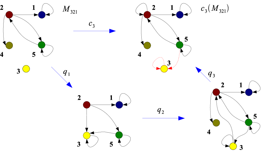
Example.$\square$We finish this section considering sequence $s_{3}=q_{3};q_{2};q_{1}$ again, calculating its composition $c_{3}$ and comparing its result with that of $s_{3}$. Recall that $S^{E}\left(s_{3}\right)=\sum_{i=1}^{3}\left(r_{i}^{E}-e_{i}^{E}\right)=r_{+}^{E}-e_{-}^{E}$.

$$\sum_{i=1}^{3}r_{i}^{E}=\left[\begin{array}[]{cccccc}\vskip-6.0pt1&1&0&0&1&|\;2\\ \vskip-6.0pt1&1&0&0&0&|\;3\\ \vskip-6.0pt1&1&1&0&0&|\;5\\ \vskip-6.0pt0&0&0&0&0&|\;1\\ \vskip-6.0pt0&0&0&0&0&|\;4\\ \end{array}\right]\quad\sum_{i=1}^{3}e_{i}^{E}=\left[\begin{array}[]{cccccc}\vskip-6.0pt0&1&0&0&1&|\;2\\ \vskip-6.0pt1&0&0&0&0&|\;3\\ \vskip-6.0pt1&0&1&0&0&|\;5\\ \vskip-6.0pt0&0&0&1&0&|\;1\\ \vskip-6.0pt0&0&0&0&0&|\;4\\ \end{array}\right]$$

$$S^{E}\left(s_{3}\right)\!=\!\left[\begin{array}[]{ccccc}\vskip-6.0pt1&0&0&0&0\\ \vskip-6.0pt0&1&0&0&0\\ \vskip-6.0pt0&1&0&0&0\\ \vskip-6.0pt0&0&0&-1&0\\ \vskip-6.0pt0&0&0&0&0\\ \end{array}\right]\!=\!\left[\begin{array}[]{ccccc}\vskip-6.0pt1&0&0&0&0\\ \vskip-6.0pt0&1&0&0&0\\ \vskip-6.0pt0&1&0&0&0\\ \vskip-6.0pt0&0&0&0&0\\ \vskip-6.0pt0&0&0&0&0\\ \end{array}\right]\!\!-\!\!\left[\begin{array}[]{ccccc}\vskip-6.0pt0&0&0&0&0\\ \vskip-6.0pt0&0&0&0&0\\ \vskip-6.0pt0&0&0&0&0\\ \vskip-6.0pt0&0&0&1&0\\ \vskip-6.0pt0&0&0&0&0\\ \end{array}\right]\!\!=r_{+}^{E}\!-\!e_{-}^{E}.$$

Sequence $s_{3}$ has been chosen not only to illustrate composition, but also compatibility and the sort of problems that may arise if it is not fulfilled. In this case, $q_{3}$ deletes node 3 and edge (3,2) but does not specify anything about edges (3,3) and (3,5) – the red dotted elements in Fig. 48 –. In order to apply the composition, either the composed production is changed by considering these elements or elements have to be related in other way (in this case, unrelated). $\blacksquare$

Previous example provides us with some clues on how the match could be defined. The basic idea is to introduce an operator over the set of productions, so once a match identifies a place in the host graph where the rule might be applied, the operator modifies the rule enlarging the deletion matrix. This way no dangling edge appears (it should enlarge the grammar rule to include the context of the original rule in the graph, adding all elements on both LHS and RHS). In essence, a match should be an injective morphism (in Matrix Graph Grammars) plus an operator. Pre-calculated information for coherence, sequentialization, and the like, should help and hopefully reduce the amount of calculations during runtime. We will study this in Chap. id1.

This section ends noting that, in Matrix Graph Grammars, one production is a morphism between two simple digraphs and thus it may carry out just one action on each element. When the composition of a concatenation is performed we get a single production. Suppose one production specifies the deletion of an element and another its addition, the overall mathematical result of the composition should leave the element unaltered. When a match is considered, depending on the chosen approach, all dangling edges incident to those erased nodes should be removed, establishing an important difference between a sequence and its composition.

26 Summary and Conclusions

Minimal and negative initial digraphs are of fundamental importance, demanding the minimal (maximal) set of elements that must be found (must not be found) in order to apply the sequence under consideration. In particular they will be used to give one characterization of the applicability problem (problem 1).

Also, composition and the main differences between this and concatenation have been addressed. Composition can be a useful tool to study concurrency. Recall from Sec. 25 that differences in the image of the composition are not due to the order in which operations are performed but in those elements needed by the productions, i.e. in the initial digraph. This also gives information on initial digraphs and its calculation. This topic – which we call G-congruence – will be addressed in deeper detail in Sec. 32.

So far we have developed some analytical techniques independent (to some extent) of the initial state of the system to which the grammar rules will be applied. This allows us to obtain information about grammar rules themselves, for example at design time. This information may be useful during runtime. We will return to this point in future chapters.

Chapter id1 starts with the semantics of a grammar rule application, so a host graph or initial state will be considered. Among other things the fundamental concept of direct derivation is introduced. We will see what can be recovered of what we have developed so far and how it can be used.

Chapter Matching

There are two fundamental parts in a grammar: Actions to be performed in every single step (grammar rules) and where these actions are to be performed in a system (matching). Previous chapter deals with the former and this chapter with the latter. Also, restrictions on the applicability of rules and their embedding in the host graph need to be addressed. This topic is studied in Chap. id1.

If a rule is applied we automatically have the pair (production, match) – normally called direct derivation – which in essence specifies what to do and where to do it. If instead of a single rule we consider a sequence with their corresponding matches then we will speak of derivation. These initial definitions, together with the matching are studied in Sec. 27 in which we will make use of some functional analysis notation (see Sec. 8). When a match is considered, there is the possibility that a new production (so called $\varepsilon$-production) is concatenated to the original one. Both productions must be applied (matched) to the same nodes. The mechanism to obtain this effect can be found in Sec. 28 (marking). An important issue is to study to what extent the notions introduced at specification time (coherence, composition, etc) can be recovered when a host graph is considered. They will be revisited considering minimal and negative initial digraphs (see Secs. 23 and 24) in a wider context in Sec. 29. A classification of $\varepsilon$-productions – helpful in Chap. id1 – is accomplished in Sec. 30. The chapter ends with a summary in Sec. 31.

27 Match and Extended Match

Matching is the operation of identifying the LHS of a rule inside a host graph. This identification is not necessarily unique, becoming one source of non determinism. The match can be considered as one of the ways of completing $L$ with respect to $G$.

Definition 27.1 (Match)

Given a production $p:L\rightarrow R$ and a simple digraph $G$, any tuple $m=\left(m_{L},m_{K}\right)$ is called a match (for $p$ in $G$), with $m_{L}:L\rightarrow G$ and $m_{K}:K^{E}\rightarrow\overline{G^{E}}$ total injective morphisms. Besides,

$$m_{L}(n)=m_{K}(n),\forall n\in L^{N}.$$ (154)

The two main differences with respect to matches as defined in the literature is that Def. 27.1 demands the non-existence of potential problematic elements and that $m$ must be injective.

It is useful to consider the structure defined by the negation of the host graph, $\overline{G}=(\overline{G^{E}},\overline{G^{N}})$. It is made up of the graph $\overline{G^{E}}$ and the vector of nodes $\overline{G^{N}}$. Note that the negation of a graph (both, the adjacency matrix and the node vector) is not a graph because in general compatibility will fail. Of course, the adjacency matrix alone $\left(\,\overline{G^{E}}\,\right)$ does define a graph.

The negation of a graph is equivalent to taking its complement. In general this complement will be taken inside some “bigger graph”, normally constructed by performing the completion with respect to other graphs involved in the operations. For example, when checking if graph $A$ is in $\overline{G^{E}}$ (suppose that $A$ has a node that is not in $G$) we obtain that $A$ cannot be found in $\overline{G^{E}}$, unless $\overline{G^{E}}$ is previously completed with that node and all its incident edges.

Notice that the negation of a graph $G$ coincides with its complement. Probably it should be more appropriate to keep the negation symbol (the overline) when there is no completion (in other words, complement is taken with respect to the graph itself) and use ^c when other graphs are involved. From now on the overline will be used in all cases. This abuse of notation should not be confusing.

Next, a notion of direct derivation that covers not only elements that must be present ($L$) but also those that should not appear ($K$) is presented. This extends the concept of derivation found in the literature, which only considers explicitly positive information.

Figure 49: Production Plus Match (Direct Derivation)

Definition 27.2 (Direct Derivation)

Given a production $p:L\rightarrow R$ as in Fig. 49 and a match $m=\left(m_{L},m_{K}\right)$, $d=\left(p,m\right)$ is called a direct derivation with result $H=p^{*}\left(G\right)$ if the square is a pushout:

$$m^{*}_{L}\circ p\left(L\right)=p^{*}\circ m_{L}\left(L\right).$$ (155)

The standard notation in this case is $G\stackrel{{\scriptstyle(p,m)}}{{\Longrightarrow}}H$, or even $G\Longrightarrow H$ if $p$, $m$ or both are not relevant.

We will see below that it is not necessary to rely on category theory to define direct derivations in Matrix Graph Grammars. It is included to ease comparison with DPO and SPO approaches.

Figure 49 displays a production $p$ and a match $m$ for $p$ in G. It is possible to close the diagram making it commutative $\left(m^{*}\circ p=p^{*}\circ m\right)$, using the pushout construction (see [22]) on category Graph^P of simple digraphs and partial functions. This categorical construction for relational graph rewriting is carried out in [52]. See Sec. 16 for a quick overview on the relational approach.

If a concatenation $s=p_{n};\ldots;p_{1}$ is considered together with the set of matchings $m=\{m_{1},\ldots,m_{n}\}$, then $d=\left(s,m\right)$ is a derivation. In this case the notation $G\Longrightarrow^{*}H$ is used.

When applying a rule to a host graph, the main problem to concentrate on is that of so-called dangling edges, which is differently addressed in DPO and SPO (see Secs. 11 and 12). In DPO, if one edge comes to be dangling then the rule is not applicable for that match. SPO allows the production to be applied by deleting any dangling edge.

For Matrix Graph Grammars we propose an SPO-like behaviour as in our case a DPO-like behaviour would be a particular case if compatibility is considered as an application condition (see Chap. id1).

Figure 50: (a) Neighborhood. (b) Extended Match

Figure 50 shows our strategy to handle dangling edges:

1. Complete $L$ with respect to $G$ ($c$ and $c^{*}$ to the left of Fig. 50). It is necessary to match $L$ in $G$ to this end.

2. Morphism $m_{L}$ will identify rule’s left hand side (after completion) in the host graph.

3. A neighborhood of $m(L)\subseteq G$ covering all relevant extra elements is selected taking into account all dangling edges not considered by match $m_{L}$ with their corresponding source and target nodes. This is performed by a morphism to be studied later, represented by $m_{\varepsilon}$.

4. Finally, $p$ is enlarged erasing any potential dangling edge. This is carried out by an operator that we will write as $T_{\varepsilon}$. See definition below on p. 27.

The order of previous steps is important as potential dangling elements must be identified and erased before any node is deleted by the original rule.

The coproduct in Fig. 50 should be understood as a means to couple $L$ and $G$. The existence of a morphism $p^{*}$ that closes the top square on the right of Fig. 50 is not guaranteed. This is where $m_{\varepsilon}$ comes in. This mapping, as explained in point 2 above, extends the production to consider any edge to distance 1 from nodes appearing in the left hand side of $p$.

Note that if it is possible to define $p^{*}$ (to close the square) then $m_{\varepsilon}$ would be the identity, and vice versa. In other words, if there are no dangling edges then it is possible to make the top square in Fig. 49 commute and, hence, it is not necessary to carry out any production “continuation”. The converse is also true.

Figure 51: Match Plus Potential Dangling Edges

Let be given a production $p:L\rightarrow R$, a host graph $G$ and a match $m:L\rightarrow G$. The graph $\Gamma$ is the set of dangling edges together with their source and target nodes. Abusing a little bit of the notation (justified by the pushout construction in Fig. 51) we will write $\Gamma\cup m(L)$ for the graph consisting of the image of $L$ by the match plus its potential dangling edges (and any incident node). Recall nihilation matrix definition, especially Lemma 21.2.

Definition 27.3 (Extended Match)

With notation as above (refer also to Fig. 50), the extended match $\widehat{m}:L+G\rightarrow G$ is a morphism with image $\Gamma\cup m\left(L\right)$.

As commented above, coproduct in Fig. 50 is used just for coupling $L$ and $G$, being the first embedded into the second by morphism $m_{L}$. We will use the notation

$$\underline{L}\stackrel{{\scriptstyle def}}{{=}}m_{G}\left(L\right)\stackrel{{\scriptstyle def}}{{=}}\left(m_{\varepsilon}\circ m\right)\left(L\right)$$ (156)

when the image of the LHS is extended with its potential dangling edges, i.e. extended digraphs are underlined and defined by composing $m$ and $m_{\varepsilon}$.

Figure 52: Matching and Extended Match

Example.$\square$Consider the digraph $L_{1}$, the host graph $G$ and the morphism match depicted to the left of Fig. 52. On the top right side in the same figure $m_{1}(L_{1})$ is drawn and $m_{G}\left(L_{1}\right)$ on the bottom right side. Nodes 2 and 3 and edges $\left(2,1\right)$ and $\left(2,3\right)$ have been added to $m_{G}\left(L\right)$ which would become dangling in the image “graph” of $G$ by $p_{1}$ (as it can not be defined it has been drawn shadowed). This is why $p^{*}_{1}$ can not be defined: node $(1:C)$ would be deleted but not edges $(1:C,2:C)$ nor $(1:C,1:S)$, so $H^{\prime}$ would not be a digraph.

As commented above, the composition is performed because $m_{1}$ and $m_{\varepsilon,1}$ are functions between Boolean matrices that have been completed. $\blacksquare$

Actually it is not necessary to rely on category theory to define direct derivations. The basic idea is given precisely by that of analytical continuation. What morphism $m_{\varepsilon}$ does is to extend the left hand side of the production, i.e. it adds elements to $L$. As matches are total functions, they can not delete elements (nodes or edges) in contrast to productions.

Hence, a match can be seen as a particular type of production with left hand side $L$ and right hand side $G$. The LHS of the production is enlarged with any potential dangling edge and the same for the RHS except for edges incident to nodes deleted by the production (as they are not added to its RHS, these edges will be deleted). This way, a direct derivation would be

$$H=\widehat{p}(m(L)).$$ (157)

Advancing some material from the next section, $m$ is essentially used to mark nodes in which $p$ acts. Production $p$ is the identity in almost all elements except in some nodes (edges) marked by $m$.

The rest of the section is devoted to the interpretation of this “continuation technique” as a production, in particular that of $m_{\varepsilon}$.

Once we are able to complete the rule’s LHS we have to do the same with the rest of the rule. To this end we define an operator $T_{\varepsilon}:\mathfrak{G}\rightarrow\mathfrak{G}^{\prime}$, where $\mathfrak{G}$ is the original grammar and $\mathfrak{G}^{\prime}$ is the grammar transformed once $T_{\varepsilon}$ has modified the production. In words, $T_{\varepsilon}$ extends production $p$ such that $T_{\varepsilon}(p)$ has the same effect than $p$ but also deletes any dangling edge.

The notation that we use from now on is borrowed from functional analysis (see Sec. 8). Bringing this notation to graph grammar rules, a rule is written as $R=\left\langle L,p\right\rangle$ (separating the static and dynamic parts of the production) while the grammar rule transformation including matching is:

$$\underline{R}=\left\langle m_{G}\left(L\right),T_{\varepsilon}p\right\rangle.$$ (158)

Proposition 27.4

With notation as above, production $p$ can be extended to consider any dangling edge, $\underline{R}=\left\langle m_{G}\left(L\right),T_{\varepsilon}p\right\rangle$.

Proof
$\square$What we do is to split the identity operator in such a way that any problematic element is taken into account (erased) by the production. In some sense, we first add elements to $p$’s LHS and afterwards enlarge $p$ to delete them. Otherwise stated, $m_{G}^{*}=T_{\varepsilon}^{-1}$ and $T_{\varepsilon}^{*}=m_{G}^{-1}$, so we have:

$$R=\left\langle L,p\right\rangle=\left\langle L,\left(T_{\varepsilon}^{-1}\circ T_{\varepsilon}\right)p\right\rangle=\left\langle m_{G}\left(L\right),T_{\varepsilon}\left(p\right)\right\rangle=\underline{R}.$$

The equality $\underline{R}=R$ is valid only for edges as $\underline{R}^{N}$ has the source and target nodes of the dangling edges. $\blacksquare$

The effect of a match can be interpreted as a new production concatenated to the original production. Let $p_{\varepsilon}\stackrel{{\scriptstyle def}}{{=}}T^{*}_{\varepsilon}$,

$$\underline{R}=\left\langle m_{G}\left(L\right),T_{\varepsilon}\left(p\right)\right\rangle = \left\langle T_{\varepsilon}^{*}\left(m_{G}\left(L\right)\right),p\right\rangle=$$ (159)

$$= p\left(T_{\varepsilon}^{*}\left(m_{G}\left(L\right)\right)\right)=p\,;\,p_{\varepsilon}\,;\,m_{G}\left(L\right)=p\,;\,p_{\varepsilon}\left(\underline{L}\right).$$

Production $p_{\varepsilon}$ is the $\varepsilon$-production associated to production $p$. Its aim is to delete potential dangling edges. The dynamic definition of $p_{\varepsilon}$ is given in (160) and (161).

The fact of taking the match into account can be interpreted as a temporary modification of the grammar, so it can be said that the grammar modifies the host graph and the host graph interacts with the grammar (altering it temporarily).

If we think of $m_{G}$ and $T_{\varepsilon}^{*}$ as productions respectively applied to $L$ and $m_{G}\left(L\right)$, it is necessary to specify their erasing and addition matrices. To this end, recall matrix $\overline{D}$ defined in Lemma 21.2, with elements in row $i$ and column $i$ equal to one if node $i$ is to be erased by $p$ and zero otherwise, which considers any potential dangling edge.

For $m_{G}$ we have that $\underline{e}^{N}=\underline{e}^{E}=0$, and $\underline{r}=\underline{L}\,\overline{L}$ (for both nodes and edges), as the production has to add the elements in $\underline{L}$ that are not present in $L$. Let $p_{\varepsilon}=\left(e^{E}_{T_{\varepsilon}},r^{E}_{T_{\varepsilon}},e^{N}_{T_{\varepsilon}},r^{N}_{T_{\varepsilon}}\right)$, then

$$e^{N}_{T_{\varepsilon}} = r^{E}_{T_{\varepsilon}}=r^{N}_{T_{\varepsilon}}=0$$ (160)

$$e^{E}_{T_{\varepsilon}} = \overline{D}\wedge\underline{L}^{E}.$$ (161)

Example.$\square$Consider rules depicted in Fig. 53, in which serverDown is applied to model a server failure. We have:

$$e^{E}=r^{E}=L^{E}=\left[\begin{array}[]{c|c}0&\,1\\ \end{array}\right];\quad e^{N}=\left[\begin{array}[]{c|c}1&\,1\\ \end{array}\right]$$

$$r^{N}=\left[\begin{array}[]{c|c}0&\,1\\ \end{array}\right];\quad L^{N}=\left[\begin{array}[]{c|c}1&\,1\\ \end{array}\right];\quad R^{E}=R^{N}=\emptyset.$$

Once $m_{G}=\left(L^{E},L^{N},\underline{r}^{E},0,0,0\right)$ and operator $T_{\varepsilon}$ have been applied, giving rise to $p_{\varepsilon}=\left(\underline{L}^{E},\underline{L}^{N},0,0,e^{E}_{T_{\varepsilon}},0\right)$, the resulting matrices are:

$$\underline{r}^{E}=\left[\begin{array}[]{ccc}\vskip-6.0pt0&0&0\\ \vskip-6.0pt1&0&0\\ \vskip-6.0pt1&0&0\\ \end{array}\right],\;\underline{L}^{E}=\left[\begin{array}[]{ccc}\vskip-6.0pt0&0&0\\ \vskip-6.0pt1&0&0\\ \vskip-6.0pt1&0&0\\ \end{array}\right],\;\underline{R}^{E}=\left[\begin{array}[]{cc}\vskip-6.0pt0&0\\ \vskip-6.0pt0&0\\ \end{array}\right],\;e_{T_{\varepsilon}}^{E}=\left[\begin{array}[]{ccc}\vskip-6.0pt0&0&0\\ \vskip-6.0pt1&0&0\\ \vskip-6.0pt1&0&0\\ \end{array}\right],$$

where ordering of nodes is $[1:S,1:C,2:C]$ for matrices $\underline{r}^{E}$, $\underline{L}^{E}$ and $e_{T_{\varepsilon}}^{E}$ and $[1:C,2:C]$ for $\underline{R}^{E}$. Matrix $\underline{r}^{E}$, besides edges added by the production, specifies those to be added by $m_{G}$ to the LHS in order to consider any potential dangling edge (in this case $\left(1:C,1:S\right)$ and $\left(2:C,1:S\right)$). As neither $m_{G}$ nor production serverDown delete any element, $\underline{e}^{E}=0$. Finally, $p_{\varepsilon}$ removes all potential dangling edges (check out matrix $e_{T_{\varepsilon}}^{E}$) but it does not add any, so $r_{T_{\varepsilon}}^{E}=0$. Vectors for nodes have been omitted. $\blacksquare$

Figure 53: Full Production and Application

Let $T^{*}_{\varepsilon}=\left({T^{*}_{\varepsilon}}^{N},{T^{*}_{\varepsilon}}^{E}\right)$ be the adjoint operator of $T_{\varepsilon}$. We will end this section giving an explicit formula for $T^{*}_{\varepsilon}$. Define $e^{E}_{\varepsilon}$ and $r^{E}_{\varepsilon}$ respectively as the erasing and addition matrices of $T_{\varepsilon}\left(p\right)$. It is clear that $r^{E}_{\varepsilon}=\underline{r}^{E}=r^{E}$ and $e^{E}_{\varepsilon}=e^{E}\vee\overline{D}\,\underline{L}^{E}$, so

$$\underline{R}^{E} = \left\langle\,\underline{L}^{E},T_{\varepsilon}\left(p\right)\,\right\rangle=r_{\varepsilon}^{E}\vee\overline{e_{\varepsilon}^{E}}\,\underline{L}^{E}=r^{E}\vee\overline{\left(e^{E}\vee\overline{D}\,\underline{L}^{E}\right)}\,\underline{L}^{E}=$$ (162)

$$= r^{E}\vee\left(D\vee\overline{\underline{L}^{E}}\right)\overline{e^{E}}\underline{L}^{E}=r^{E}\vee\overline{e^{E}}D\underline{L}^{E}.$$

Previous identities show that $\underline{R}^{E}=\left\langle\underline{L}^{E},T_{\varepsilon}^{E}\left(p^{E}\right)\right\rangle=\left\langle D\,\underline{L}^{E},p^{E}\right\rangle$, which proves the identity:

$$T^{*}_{\varepsilon}=\left({T^{*}_{\varepsilon}}^{N},{T^{*}_{\varepsilon}}^{E}\right)=\left(id,D\right).$$ (163)

Summarizing, when a match $m$ is considered for a production $p$, the production itself is first modified in order to consider all potential dangling edges. Morphism $m$ is automatically transformed into a match which is free from any dangling element and, in a second step, a pre-production $p_{\varepsilon}$ is appended to form the concatenation

$$\widehat{p}^{*}=p^{*}\,;p^{*}_{\varepsilon}.$$ (164)

Note that as injectiveness of matches is demanded, there is no problem such as elements identified by matches that are both kept and deleted.

Depending on the operator $T_{\varepsilon}$, side effects are permitted (SPO-like behaviour) or not (DPO-like behaviour). A fixed grammar or fixed Matrix Graph Grammar is one in which (mandatory) the operator $T_{\varepsilon}$ is the identity. If the operator is not forced to be the identity, we will speak of a floating grammar or floating Matrix Graph Grammar. Notice that the existence of side effects is equivalent to transforming a production into a sequence. This will also be the case when we deal with graph constraints and application conditions (Chap. id1).

28 Marking

In previous section the problem of dangling edges has been addressed by adding an $\varepsilon$-production which deletes any problematic edge, so the original rule can be applied as it is. However there is no way to guarantee that both productions will use the same elements (recall that in general matches are non-deterministic). The same problem exists with application conditions (Sec. 39) or whenever a rule is split into subrules and applying them to the same elements in the host graph is desired.

This topic is studied in [73] (for a different reason) and the solution proposed there is to ‘‘pass’’ the match from one production to the other. We will tackle this problem in a different way that consists in defining an operator $T_{\mu,\alpha}$ for a label $\alpha$ acting on production $p$ as follows:

• If no node is typed $\alpha$ in $p$ then a new node labeled $\alpha$ is added and connected to every already existing node.

• If, on the contrary, there exists a node of that type then it is deleted.

The basic idea is to mark nodes and related productions with a node of type $\alpha$. The operator behaves differently depending on whether it is marking the state (it adds node $\alpha$) or it is extending the productions ($\alpha$-typed nodes are removed).

For an example of a short sequence of two productions, please refer to Fig. 54. Using functional analysis notation:

$$R=\left\langle L,p\right\rangle\longmapsto\underline{R}=\left\langle m_{\varepsilon}(L),T_{\varepsilon}(p)\right\rangle\longmapsto\underline{\underline{R}}=\left\langle m_{\varepsilon}(L),T_{\mu}\circ T_{\varepsilon}(p)\right\rangle$$ (165)

where, as in Sec. 27, $\underline{R}$ is the extended rule’s RHS that considers any dangling edge.

If a production is split into two subproductions, say $p\longmapsto T_{\varepsilon}(p)=p\,;p_{\varepsilon}$ and we want them to be applied in the same nodes of the host graph, we may proceed as follows:

• Enlarge $p_{\varepsilon}$ to add one node of some non-existent type ($\alpha$) together with edges starting in this node and ending in nodes used by $p_{\varepsilon}$.

• Enlarge $p$ to delete $\alpha$ nodes of previous step.

It is important to note that $p$ must be enlarged to delete only the previously added node ($\alpha$) and not the edges starting in $\alpha$ appended by $T_{\mu}$ to $p_{\varepsilon}$. The reason is that in case of a sequence in which the $\varepsilon$-production is advanced several positions, there exists the possibility to create unreal dependencies between $p$ and some production applied before $p$ but after $p_{\varepsilon}$ (the example below illustrates this point in particular).

Marking will normally create new $\varepsilon$-productions related to $p$. Note however that no recursive process should arise as there shouldn’t be any interest in permuting (advancing) this new $\varepsilon$-productions.

For $\varepsilon$-productions all this makes sense just in case we do not compose $p\circ p_{\varepsilon}$ (no marking would be needed). Two different operators, one for $\alpha$ nodes addition and another for $\alpha$ nodes deletion (instead of just one) are not defined because marking always acts on different productions. This should not cause any confusion.

Figure 54: Example of Marking and Sequence $s=p;p_{\varepsilon}$

Example.$\square$Figure 54 illustrates the process for a simple production $p$ that deletes node 1 and is applied to a host graph in which one or two dangling edges (depending on the match, $1$ or $1^{\prime}$) would be generated, $(1,2)$ or $(1^{\prime},2)$ and $(1^{\prime},3)$.

We have chosen node $1$ for the match so there should be one dangling edge $(1,2)$. In order to avoid it, an $\varepsilon$-production $p_{\varepsilon}$ which deletes $(1,2)$ is appended to $p$.

The marking process modifies $p_{\varepsilon}$ and $p$ becoming $p_{\varepsilon}\mapsto T_{\mu}(p_{\varepsilon})$ and $p\mapsto T_{\mu}(p)$, respectively. Note that $T_{\mu}(p)$ generates two dangling edges – $(\alpha,1)$ and $(\alpha,2)$ – so a new $\varepsilon$-production $p^{\prime}_{\varepsilon}$ ought to be added.

When the production is applied, a sequence is generated as operators act on the production – $p\mapsto T_{\varepsilon}(p)\mapsto T_{\mu}\circ T_{\varepsilon}(p)\mapsto T_{\varepsilon}\circ T_{\mu}\circ T_{\varepsilon}(p)$ – giving rise to the following sequence of productions:

$$p\longmapsto p\,;p_{\varepsilon}\longmapsto T_{\mu}(p);p^{\prime}_{\varepsilon};T_{\mu}(p_{\varepsilon}).$$ (166)

The reason why it is important to specify only the new node deletion ($\alpha$) and not the edges starting in this node is not difficult but might be a bit subtle. It has been mentioned above. The rest of the example is devoted to explaining it.

If we specified the edges also, say $(\alpha,1)$ and $(\alpha,2)$ as above, then the transformed production $T_{\mu}(p)$ would use node 2 as it should appear in its LHS and RHS (remember that $p$ did not act on node $2$).

Now imagine that we are interested in advancing the $\varepsilon$-production three positions, for example because we know that it is external (see Sec. 30) and independent: $p\,;p_{\varepsilon};p_{2};p_{1}\mapsto p\,;p_{2};p_{1};p_{\varepsilon}$. Suppose that production $p_{1}$ (placed between $p$ and the new allocation of $p_{\varepsilon}$) deletes node 2 and production $p_{2}$ adds it. If $p$ was sequential independent with respect to $p_{1}$ and $p_{2}$ then it would not be anymore due to the edge ending in node $2$ because now $p$ would use node $2$ (appears in its left and right hand sides). $\blacksquare$

Note that as the marking process can be easily automated, we can safely ignore it and assume that it is somehow being performed, by some runtime environment for example.

29 Initial Digraph Set and Negative Digraph Set

Concerning minimal and negative initial digraphs there may be different ways to complete rule matrices, depending on the matches. Therefore, we no longer have a unique initial digraph but a set (if we assume any possible match). In fact two sets, one for elements that must be found in the host graph and another for those that must be found in its complement. This section is closely related to Secs. 23 and 24 and extends results therein proved.

The initial digraph set contains all graphs that can be potentially identified by matches in concrete host graphs.

Definition 29.1 (Initial Digraph Set)

Given sequence $s_{n}$, its associated initial digraph set $\mathfrak{M}\left(s_{n}\right)$ is the set of simple digraphs $M_{i}$ such that $\forall M_{i}\in\mathfrak{M}\left(s_{n}\right)$:

1. $M_{i}$ has enough nodes and edges for every production of the concatenation to be applied in the specified order.

2. $M_{i}$ has no proper subgraph with previous property (keeping identifications).

Every element $M_{i}\in\mathfrak{M}\left(s_{n}\right)$ is said to be an initial digraph for $s_{n}$. It is easy to see that $\forall s_{n}$ finite sequence of productions we have $\mathfrak{M}\left(s_{n}\right)\neq\emptyset$.

In Sec. 20 coherence was used in a more or less absolute way when dealing with sequences, assuming some horizontal identification of elements. Now we see that, due to matching, coherence is a property that may depend on the given initial digraph so, depending on the context, it might be appropriate to say that $s_{n}$ is coherent with respect to initial digraph $M_{i}$ (just in case direct derivations are considered). Note that what we fix by choosing an initial digraph is the relative matching of nodes across productions (one of the actions of completion).

For the initial digraph set we can define the maximal initial digraph as the element $M_{n}\in\mathfrak{M}\left(s_{n}\right)$ that considers all nodes in $p_{i}$ to be different. This element is unique up to isomorphism, and corresponds to considering the parallel application of every production in the sequence, i.e. the LHS of every production in the sequence is matched in disjoint parts of the host graph.

This concept has already been used although it was not explicitly mentioned: In the proof of Theorem 23.2 we started with $\bigvee_{i=1}^{n}L_{i}$, a digraph that had enough nodes to perform all actions specified by the sequence.

In a similar way, $M_{i}\in\mathfrak{M}\left(s_{n}\right)$ in which all possible identifications are performed are known as minimal initial digraphs. Contrary to the maximal initial digraph, minimal initial digraphs need not be unique as the following example shows.

Figure 55: Initial Digraph Set for s=remove_channel;remove_channel

Example.$\square$In Figure 55 we have represented the minimal digraph set for the sequence s = removeChannel;removeChannel. The production is also depicted in the figure where S stands for server and C for client. Note that it is not coherent if all nodes in $L_{3}$ are identified because the link between two clients is deleted twice. Therefore, the initial digraphs should provide at least (in fact, at most) two different links between clients.

In the figure, the maximal initial digraph is $M_{7}$ and $M_{1}$ and $M_{3}$ are the two minimal initial digraphs. Identifications are written as $i=j$ meaning that nodes $i$ and $j$ become one and the same. A top-bottom procedure has been followed, starting out with the biggest digraph $M_{7}$ and ending in the smallest. Numbers on labels are all different to ease identifications on the initial digraph tree to the right of Fig. 55. $\blacksquare$

We can provide $\mathfrak{M}\left(s_{n}\right)$ with some structure $\mathfrak{T}\left(s_{n}\right)$. See the right side of Fig. 55. Every node in $\mathfrak{T}$ represents an element of $\mathfrak{M}$. A directed edge from one node to another stands for one operation of identification between corresponding nodes in the LHS and RHS of productions of the sequence $s_{n}$.

Following with the example above, node $M_{7}$ is the maximal initial digraph, as it only has outgoing edges. Nodes $M_{1}$ and $M_{3}$ are minimal as they only have ingoing edges. The structure $\mathfrak{T}$ is an acyclic digraph with single root node (recall that there is just one maximal initial digraph), known as graph-structured stack.

It is possible to make a similar construction for negative initial digraphs that we will call negative initial set. It will be represented by $\mathfrak{N}(s_{n})$ where $s_{n}$ is the sequence under study.

Figure 56: Negative Digraph Set for s=clientDown;clientDown

Definition 29.2 (Negative Initial Set)

Given sequence $s_{n}$, its associated negative initial set $\mathfrak{N}\left(s_{n}\right)$ is the set of simple digraphs $K_{i}$ such that $\forall K_{i}\in\mathfrak{N}\left(s_{n}\right)$:

1. $K_{i}$ specifies all edges that can potentially prevent the application of some production of $s_{n}$.

2. $K_{i}$ has no proper subgraph with previous property (keeping identifications).

Example.$\square$We study the sequence s=clientDown;clientDown very similar to that in the example of p. 55 but deleting one node and two edges. It is depicted in Fig. 56 and represents the failure of a client connected to a server and to another client.

The same labeling criteria has been followed to ease comparison. Minimal digraphs are very similar to those in Fig. 55 and in fact identifications have been performed such that $K_{i}$ corresponds to $M_{i}$. Graphs do not include all edges that should not appear because there would be many edges, probably being a confusing instead of a clarifying example. For instance, in $K_{4}$ there can not be any edge incident to node $(6:C)$ (except those coming from $(1:S)$ and $(4:S)$), in particular edge $(2:C,6:C)$ which is not represented. Complete graph $K_{4}$ can be found in Fig. 57. Note that for $K_{4}$ the order of deletion is important, first node $(2:C)$ and then node $(3:C)$. $\blacksquare$

Figure 57: Complete Negative Initial Digraph $K_{4}$

The relationship between elements in $\mathfrak{M}$ and $\mathfrak{N}$ is compiled in Corollary 25.2. Note that the cardinality of both sets do not necessarily coincide. In the example of p. 55, production $s$ does not add any edge nor deletes any node (hence, no forbidden element) so its negative digraph set is empty.

Although in this book we are staying at a more theoretical level, we will make a small digression on application of these concepts and possible implementations.

Let’s take as an example the calculation of $M_{0}$ in Proposition 34.2, which states that two derivations $d$ and $d^{\prime}$ are sequential independent if they have a common initial digraph for some identification of nodes, i.e. if $\mathfrak{M}(d)\cap\mathfrak{M}(d^{\prime})\neq\emptyset$. We see that it is possible to follow two complementary approaches:

• Top-bottom. Begin with the maximal initial digraph and start identifying elements until we get the desired initial digraph or eventually get a contradiction.

• Bottom-up. Start with different initial digraphs and unrelate nodes until an answer is reached.

In Fig. 55 on p. 55 either we begin with $M_{7}$ and start identifying nodes, eventually getting any element of the minimal initial set, or we start with $M_{1}$ – which is not necessarily unique – and build up the whole set, or stop as soon as we get the desired minimal initial digraph.

Let the matrix filled up with 1’s in all positions be represented by 1. For the first case the following identity may be of some help:

$$M_{d}=M_{d^{\prime}}\Leftrightarrow M_{d}M_{d^{\prime}}\vee\overline{M}_{d}\overline{M}_{d^{\prime}}=1.$$ (167)

A SAT solver can be used on (167) to obtain conditions, setting all elements in $M$ as variables except those already known. In order to store $M$, binary decision diagrams – BDD – can be employed. Refer to [8].

The same alternative processes might be applied to the negative initial set to eventually reach any of its elements.

30 Internal and External $\varepsilon$-productions

Dangling edges can be classified into two disjoint sets according to the place where they appear, whether they have been added by a previous production or not.

For example, given the sequence $p_{2};p_{1}$, suppose that rule $p_{1}$ uses but does not delete edge $\left(4,1\right)$, that rule $p_{2}$ specifies the deletion of node $1$ and that we have identified both nodes $1$. It is mandatory to add one $\varepsilon$-production $p_{\varepsilon,2}$ to the grammar with the disadvantage that there is an unavoidable problem of coherence between $p_{1}$ and $p_{\varepsilon,2}$ if we wanted to advance the application of $p_{\varepsilon,2}$ to $p_{1}$, i.e. they are sequentially dependent.

Hence, edges of $\varepsilon$-productions are of two different types:

• External: Any edge not appearing explicitly in the grammar rules, i.e. edges of the host graph ‘‘in the surroundings’’ of the actual initial digraph. Examples are edges $\left(1:C,1:S\right)$ and $\left(2:C,1:S\right)$ in Fig. 53 on p. 53.

• Internal: Any edge used or appended by a previous production in the concatenation. One example is edge $\left(4,1\right)$ mentioned above.

$\varepsilon$-productions can be classified in internal $\varepsilon$-productions if any of its edges is internal and external $\varepsilon$-productions otherwise.

The “advantage” of internal over external $\varepsilon$-productions is that the former can be considered (are known) during rule specification while external remain unknown until the production is applied. This, in turn, may spoil coherence, compatibility and other calculations performed during grammar definition.

On the other hand, external $\varepsilon$-productions do not interfere with grammar rules so they can be advanced to the beginning and they can even be composed to get a single production if so desired (these are called exact derivations, defined below).

Figure 58: Example of Internal and External Edges

Example.$\square$Let’s consider the derivation $d_{2}=p_{2};p_{1}$ (see Fig. 58). Edge $(1,2)$ in graph $G_{1}$ is internal (it has been added by production $p_{1}$) while edge $(2,3)$ in the same graph is external (it already existed in $G_{0}$). $\blacksquare$

Given a host graph $G$ in which $s_{n}$ – coherent and compatible – is to be applied, and assuming a match which identifies $s_{n}$’s actual initial digraph ($M_{n}$) in $G$ (defining a derivation $d_{n}$ out of $s_{n}$), we check whether for some $\widehat{m}$ and $\widehat{T_{\varepsilon}}$, which respectively represent all changes to be done to $M_{n}$ and all modifications to $s_{n}$, it is correct to write

$$H_{n}=d_{n}\left(M_{n}\right)=\left\langle\widehat{m}\left(M_{n}\right),\widehat{T_{\varepsilon}}\left(s_{n}\right)\right\rangle,$$ (168)

where $H_{n}$ is the subgraph of the final state $H$ corresponding to the image of $M_{n}$.

Equation (141) allows us to consider a concatenation almost as a production, justifying operators $\widehat{T_{\varepsilon}}$ and $\widehat{m}$ in eq. (168) and our abuse of notation (recall that bra and kets apply to productions and not to sequences).

All previous considerations together with the following example are compiled into the definition of exact sequence.

Example.$\square$Let $s_{2}=p_{2};p_{1}$ be a coherent and compatible concatenation. Using operators we can write

$$H=\left\langle m_{G,2}\left(\left\langle m_{G,1}\left(M_{2}\right),T_{\varepsilon,1}\left(p_{1}\right)\right\rangle\right),T_{\varepsilon,2}\left(p_{2}\right)\right\rangle,$$ (169)

which is equivalent to $H=p_{2};\,p_{\varepsilon,2};p_{1};\,p_{\varepsilon,1}\left(\underline{M_{2}}\right)$, with actual initial digraph twice modified $\underline{M_{2}}=m_{G,2}\left(m_{G,1}\left(M_{2}\right)\right)=\left(m_{G,2}\circ m_{G,1}\right)\left(M_{2}\right)$. $\blacksquare$

Definition 30.1 (Exact Derivation)

Let $d_{n}=\left(s_{n},m_{n}\right)$ be a derivation with actual initial digraph $M_{n}$, sequence $s_{n}=p_{n};\ldots;p_{1}$, matches $m_{n}=\{m_{G,1},\ldots,m_{G,n}\}$ and $\varepsilon$-productions $\{p_{\varepsilon,1},\ldots,p_{\varepsilon,n}\}$. It is an exact derivation if there exist $\widehat{m}$ and $\widehat{T}_{\varepsilon}$ such that equation (168) is fulfilled.

Equation (168) is satisfied if once all matches are calculated, the following identity holds:

$$p_{n};p_{\varepsilon,n};\ldots;p_{1};p_{\varepsilon,1}=p_{n};\ldots;p_{1};p_{\varepsilon,n};\ldots;p_{\varepsilon,1}.$$ (170)

Proposition 30.2

With notation as in Def. 30.1, if $p_{\varepsilon,j}\bot\left(p_{j-1};\ldots;p_{1}\right)$, $\forall j$, then $d_{n}$ is exact.

Proof
$\square$Operator $\widehat{T_{\varepsilon}}$ modifies the sequence adding a unique $\varepsilon$-production, the composition of all $\varepsilon$-productions $p_{\varepsilon,i}$. To see this, if one edge is to dangle, it should be eliminated by the corresponding $\varepsilon$-production so no other $\varepsilon$-production deletes it unless it is added by a subsequent production. But by hypothesis there is sequential independence of every $p_{\varepsilon,j}$ with respect to all preceding productions and hence $p_{\varepsilon,j}$ does not delete any edge used by $p_{j-1},\ldots,p_{1}$. In particular no edge added by any of these productions is erased.

In Def. 30.1, $\widehat{m}$ is the extension of the match $m$ which identifies the actual initial digraph in the host graph, so it adds to $m\left(M_{n}\right)$ all nodes and edges to distance one to nodes that are going to be erased. A symmetrical reasoning to that of $\widehat{T_{\varepsilon}}$ shows that $\widehat{m}$ is the composition of all $m_{G,i}$. $\blacksquare$

With Def. 30.1 and Prop. 30.2 it is feasible to obtain a concatenation where all $\varepsilon$-productions are applied first, and all grammar rules afterwards, recovering the original concatenation. Despite some obvious advantages, all dangling edges are deleted at the beginning which may be counterintuitive or even undesired if, for example, the deletion of a particular edge is used for synchronization purposes.

The following corollary states that exactness can only be ruined by internal $\varepsilon$-productions.

Corollary 30.3

Let $s_{n}$ be a sequence to be applied to a host graph $G$ and $M_{k}\in\mathfrak{M}\left(s_{n}\right)$. Assume there exists at least one match in $G$ for $M_{k}$ that does not add any internal $\varepsilon$-production. Then, $d_{n}$ is exact.

Proof (sketch)
$\square$All potential dangling elements are edges surrounding the actual initial digraph. It is thus possible to adapt the part of the host graph modified by the sequence at the beginning, so applying Prop. 30.2 we get exactness. $\blacksquare$

We are now in the position to characterize applicability, problem 1 stated on p. 1. In essence, applicability characterizes when a sequence is a derivation with respect to a given initial graph.

Theorem 30.4 (Applicability Characterization)

A sequence $s_{n}$ is applicable to $G$ if there are matches for every production (define the derivation $d_{n}$ as the sequence $s_{n}$ plus these matches) such that any of the two following equivalent conditions is fulfilled:

• Derivation $d_{n}$ is coherent and compatible.

• $d_{n}$’s minimal initial digraph is in $G$ and $d_{n}$’s negative initial digraph is in $\overline{G}$.

Proof
$\square$$\blacksquare$

31 Summary and Conclusions

In this chapter we have seen how it is possible to match the left hand side of a production in a given graph. We have not given a matching algorithm, but the construction of derivations out of productions.

There are two properties that we would like to highlight. The expressive power of Matrix Graph Grammars lies in between that of other approaches such as DPO and SPO:

• We find it more intuitive and convenient to demand injectiveness on matches. This can be seen as a limitation on the semantics of the grammar but, on the other hand, not asking for injectiveness might present a serious problem. For example, when injectivity is necessary for some rules or non-injectivity is not allowed in some parts of the host graph. In a limit situation, it can be the case that several nodes and edges collapse to a single node and a single edge.

• Rules can be applied even if they do not consider every edge that can appear in some given state. The grammar designer can concentrate on the algorithm at a more abstract level, without worrying about every single case in which a concrete rule needs to be applied.

An advantage of $\varepsilon$-productions over previous approaches to dangling edges is that they are erased by productions. This increases our analysis abilities as there are no side effects.

We have also introduced marking, useful in many situations in which it is necessary to guarantee that some parts of two or more rules will be matched in the same area of the host graph. It will be used throughout the rest of the book.

Initial and negative digraph sets are a generalization of minimal and negative initial digraphs in which some or all possible identifications are considered. Actually, these concepts could have been introduced in Chap. id1, but we have postponed their study because we find it more natural to consider them once matching has been introduced.

We have classified the productions generated at runtime in internal and external. In fact, it would be more appropriate to speak of internal and external edges, but this classification suffices for our purposes.

Applicability (problem 1 stated on p. 1) will be used in Chap. id1 to characterize consistency of application conditions and graph constraints.

In the next chapter sequentialization and parallelism are studied in detail. Problem 3, sequential independence (stated on p. 3), will be addressed and, in doing so, we will touch on parallelism and related topics.

Chapter id1 generalizes graph constraints and application conditions and adapts them to Matrix Graph Grammars. This step is not necessary but convenient to study reachability, problem 4 stated on p. 4, which will be carried out in Chap. id1.

Chapter Sequentialization and Parallelism

In this chapter we will study in some detail problem 3 (sequential independence, p. 3) which is a particular case of problem 2 (independence, p. 2). Recall from Chap. id1 that two derivations $d$ and $d^{\prime}$ are independent for a given state $G$ if $d(G)=H\cong H^{\prime}=d^{\prime}(G)$. We call them sequential independent if, besides, $\exists\;\sigma$ permutation such that $d^{\prime}=\sigma(d)$.

Applicability (problem 1) is one of the premises of independence, establishing an obvious connection between them. In Chap. id1 we will sketch the relationship with reachability (problem 4) and conjecture one with confluence (problem 5) in Chap. id1.

In Sec. 32 G-congruence is presented, which in essence poses conditions for two derivations (one permutation of the other) to have the same minimal and negative initial digraphs. The idea behind sequential independence is that changes of order in the position of productions inside a sequence do not alter the result of their application. This is addressed in Sec. 33 for sequences and in Sec. 34 for derivations. If a quick review of permutation groups notation is needed, please see Sec. 6. In Sec. 35 we will see that there is a close link between sequential independence and parallelization (see Church-Rosser theorems in, e.g. [11]). As in every chapter, we will close with a summary (Sec. 36).

32 Graph Congruence

Sameness of minimal and negative initial digraphs for two sequences – one a permutation of the other – or for two derivations if some matches have been given, will be known as graph congruence or G-congruence. This concept helps in characterizing sequential independence (see Theorems 33.2 and 33.3).

Definition 32.1 (G-congruence)

Two coherent sequences $s_{n}$ and $\sigma\left(s_{n}\right)$, where $\sigma$ is a permutation, are called G-congruent if they have the same minimal and negative initial digraphs, $M(s_{n})=M(\sigma\left(s_{n}\right))$ and $K(s_{n})=K(\sigma\left(s_{n}\right))$.

We will identify the conditions that must be fulfilled in order to guarantee equality of initial digraphs, first for productions advancement and then for delaying, starting with two productions, continuing with three and four to end up setting the theorem for the general case.

The basic remark that justifies the way we tackle G-congruence is that a sequence and a permutation of it perform the same actions but in different order. Initial digraphs depend on actions and the order in which they are performed. The idea is to concentrate on how a change in the order of actions may affect initial digraphs.

Suppose we have a coherent sequence made up of two productions $s_{2}=p_{2};p_{1}$ with minimal initial digraph $M_{2}$ and, applying the (only possible) permutation $\sigma_{2}$, get another coherent concatenation $s_{2}^{\prime}=p_{1};p_{2}$ with minimal initial digraph $M_{2}^{\prime}$. Production $p_{1}$ does not delete any element added by $p_{2}$ because, otherwise, if $p_{1}$ in $s_{2}$ deleted something, it would mean that it already existed (as $p_{1}$ is applied first in $s_{2}$) while $p_{2}$ adding that same element in $s_{2}^{\prime}$ would mean that this element was not present (because $p_{2}$ is applied first in $s_{2}^{\prime}$). This condition can be written:

$$e_{1}r_{2}=0.$$ (171)

A similar reasoning states that $p_{1}$ can not add any element that $p_{2}$ is going to use:

$$r_{1}L_{2}=0.$$ (172)

Analogously for $p_{2}$ against $p_{1}$, i.e. for $s^{\prime}_{2}=p_{1};p_{2}$, we have:

$$e_{2}r_{1} = 0$$ (173)

$$r_{2}L_{1} = 0.$$ (174)

As a matter of fact two equations are redundant – (171) and (173) – because they are already contained in the other two. Note that $e_{i}L_{i}=e_{i}$, i.e. in some sense $e_{i}\subset L_{i}$, so it is enough to ask for:

$$r_{1}L_{2}\vee r_{2}L_{1}=0.$$ (175)

It is easy to check that these conditions make minimal initial digraphs coincide, $M_{2}=M_{2}^{\prime}$. In detail:

$$M_{2}=M_{2}\vee r_{1}L_{2}=L_{1}\vee\overline{r}_{1}L_{2}\vee r_{1}L_{2} = L_{1}\vee L_{2}$$

$$M^{\prime}_{2}=M^{\prime}_{2}\vee r_{2}L_{1}=L_{2}\vee\overline{r}_{2}L_{1}\vee r_{2}L_{1} = L_{2}\vee L_{1}.$$

We will very briefly compare conditions for two productions with those of the SPO approach. In references [23, 24], sequential independence is defined and categorically characterized. See also Secs. 11 and 12, in particular equations (15) and (16)). It is not difficult to translate those conditions to our matrix language:

$$r_{1}L_{2} = 0$$ (176)

$$e_{2}R_{1}\equiv e_{2}r_{1}\vee e_{2}\,\overline{e}_{1}\,L_{1} = 0.$$ (177)

First condition is eq. (172) and, as mentioned above, first part of second condition ($e_{2}r_{1}=0$) is already considered in eq. (172). Second part of second equation ($e_{2}\,\overline{e}_{1}\,L_{1}$ = 0) is demanded for coherence, in fact something a bit stronger: $e_{2}L_{1}=0$. Hence G-congruence plus coherence imply sequential independence in the SPO case, at least for a sequence of two productions. The converse does not hold in general. Our conditions are more demanding because we consider simple digraphs.

Let’s now turn to the negative initial digraph, for which the first production should not delete any element forbidden for $p_{2}$. In such a case these elements would be in $\overline{G}$ for $p_{1};p_{2}$ and in $G$ for $p_{2};p_{1}$:

$$0=e_{1}K_{2}=e_{1}r_{2}\vee e_{1}\overline{e}_{2}\overline{D}_{2}.$$ (178)

Note that we already had $e_{1}r_{2}=0$ in equation (171). A symmetrical reasoning yields $e_{2}\overline{e}_{1}\overline{D}_{1}=0$, and altogether:

$$e_{1}\overline{e}_{2}\overline{D}_{2}\vee e_{2}\overline{e}_{1}\overline{D}_{1}=0.$$ (179)

First monomial in eq. (179) simply states that no potential dangling edge for $p_{2}$ (not deleted by $p_{2}$) can be deleted by $p_{1}$. Equations (175) and (179) are schematically represented in Fig. 59.

Figure 59: G-congruence for $s_{2}=p_{2};p_{1}$

It is straightforward to show that equation (179) guarantees the same negative initial digraph. In $p_{2};p_{1}$ the negative initial digraph is given by $K_{1}\vee\overline{e}_{1}K_{2}$. Condition (178) demands $e_{1}K_{2}=0$ so we can or them to get:

$$K_{1}\vee\overline{e}_{1}K_{2}\vee e_{1}K_{2}=K_{1}\vee K_{2}.$$ (180)

A similar reasoning applies to $p_{1};p_{2}$, obtaining the same result.

We will proceed with three productions so, following a consistent notation, we set $s_{3}=p_{3};p_{2};p_{1}$, $s_{3}^{\prime}=p_{2};p_{1};p_{3}$ with permutation $\sigma_{3}=[\,1\;3\;2\,]$ and their corresponding minimal initial digraphs $M_{3}=L_{1}\vee\overline{r}_{1}\,L_{2}\vee\overline{r}_{1}\,\overline{r}_{2}\,L_{3}$ and $M_{3}^{\prime}=\overline{r}_{3}\,L_{1}\vee\overline{r}_{3}\,\overline{r}_{2}\,L_{2}\vee L_{3}$. Conditions are deduced similarly to the two productions case:

$$r_{3}L_{1}=0\qquad r_{3}L_{2}\overline{r_{1}}=0\qquad r_{1}L_{3}=0\qquad r_{2}L_{3}\overline{e_{1}}=0.$$ (181)

Let’s interpret them all. $r_{3}L_{1}=0$ says that $p_{3}$ cannot add an edge that $p_{1}$ uses. This is because this would mean (by $s_{3}$) that the edge is in the host graph (it is used by $p_{1}$) but $s^{\prime}_{3}$ says that it is not there (it is going to be added by $p_{3}$). The second condition is almost equal but with $p_{2}$ in the role of $p_{1}$, which is why we demand $p_{1}$ not to add the element $\left(\overline{r_{1}}\right)$. Third equation is symmetrical with respect to the first. The fourth equation states that we would derive a contradiction if the second production adds something $(r_{2})$ that production $p_{3}$ uses $(L_{3})$ and $p_{1}$ does not delete $\left(\overline{e_{1}}\right)$. This is because by $s_{3}$ the element was not in the host graph. Note that $s^{\prime}_{3}$ says the opposite, as $p_{3}$ (to be applied first) uses it. All can be put together in a single expression:

$$L_{3}\left(r_{1}\vee\overline{e_{1}}\,r_{2}\right)\vee r_{3}\left(L_{1}\vee\overline{r_{1}}\,L_{2}\right)=0.$$ (182)

For the sake of completeness let’s point out that there are other four conditions but they are already considered in (182):

$$e_{1}r_{3}=0\qquad r_{3}e_{2}\overline{r_{1}}=0\qquad e_{3}r_{1}=0\qquad r_{2}e_{3}\overline{e_{1}}=0.$$ (183)

Now we deal with those elements that must not be present. Four conditions similar to those for two productions – compare with equations in (178) – are needed:

$$e_{1}K_{3}=e_{1}r_{3}\vee e_{1}\overline{e}_{3}\overline{D}_{3} = 0$$

$$e_{3}K_{1}=e_{3}r_{1}\vee e_{3}\overline{e}_{1}\overline{D}_{1} = 0$$

$$e_{3}K_{2}\overline{e}_{1}=e_{3}r_{2}\overline{e}_{1}\vee e_{3}\overline{e}_{1}\overline{e}_{2}\overline{D}_{2} = 0$$

$$e_{2}K_{3}\overline{r}_{1}=e_{2}r_{3}\overline{r}_{1}\vee e_{2}\overline{r}_{1}\overline{e}_{3}\overline{D}_{3} = 0.$$ (184)

Note that the first monomial in every equation can be discarded as they are already considered in (182). We put them altogether to get:

$$e_{1}\overline{e}_{3}\overline{D}_{3} \vee e_{3}\overline{e}_{2}\overline{e}_{1}\overline{D}_{2}\vee e_{3}\overline{e}_{1}\overline{D}_{1}\vee e_{2}\overline{e}_{3}\overline{r}_{1}\overline{D}_{3}=$$ (185)

$$= e_{3}\left(\overline{e}_{1}\overline{D}_{1}\vee\overline{e}_{1}\overline{e}_{2}\overline{D}_{2}\right)\vee\overline{e}_{3}\overline{D}_{3}\left(e_{1}\vee\overline{r}_{1}e_{2}\right).$$

In Fig. 60 there is a schematic representation of all G-congruence conditions for sequences $s_{3}=p_{3};p_{2};p_{1}$ and $s^{\prime}_{3}=p_{2};p_{1};p_{3}$. These conditions guarantee sameness of the minimal and negative initial digraphs, which will be proved below, in Theorem 32.6.

Figure 60: G-congruence for Sequences $s_{3}=p_{3};p_{2};p_{1}$ and $s^{\prime}_{3}=p_{2};p_{1};p_{3}$

Moving one production three positions forward in a sequence of four productions, i.e. $p_{4};p_{3};p_{2};p_{1}\mapsto p_{3};p_{2};p_{1};p_{4}$, while maintaining the minimal initial digraph has as associated conditions those given by the equation:

$$L_{4}\left(r_{1}\vee\overline{e}_{1}\,r_{2}\vee\overline{e}_{1}\,\overline{e}_{2}\,r_{3}\right)\vee r_{4}\left(L_{1}\vee\overline{r}_{1}\,L_{2}\vee\overline{r}_{1}\,\overline{r}_{2}\,L_{3}\right)=0.$$ (186)

and for the negative initial digraph we have:

$$e_{4}\left(\overline{e}_{1}\,\overline{D}_{1}\vee\overline{e}_{1}\,\overline{e}_{2}\overline{D}_{2}\vee\overline{e}_{1}\,\overline{e}_{2}\,\overline{e}_{3}\overline{D}_{3}\right)\vee\overline{e}_{4}\,\overline{D}_{4}\left(e_{1}\vee\overline{r}_{1}\,e_{2}\vee\overline{r}_{1}\,\overline{r}_{2}\,e_{3}\right)=0.$$ (187)

Equations (186) and (187) together give G-congruence for $s_{4}$ and $s^{\prime}_{4}$ are depicted on Fig. 61.

Before moving to the general case, let’s briefly introduce and put an example of a simple notation for cycles moving forward and backward a single production:

1. Advance production $n-1$ positions: $\phi_{n}=[\,1\quad n\,\quad\,n-1\quad\ldots\quad 3\quad 2\,]$.

2. Delay production $n-1$ positions: $\delta_{n}=[\,1\quad 2\quad\ldots\quad n-1\quad n\,]$.

Figure 61: G-congruence for $s_{4}=p_{4};p_{3};p_{2};p_{1}$ and $s^{\prime}_{4}=p_{3};p_{2};p_{1};p_{4}$

Example.$\square$Consider advancing three positions the production $p_{5}$ inside the sequence $s_{5}=p_{5};p_{4};p_{3};p_{2};p_{1}$ to get $\phi_{4}\left(s_{5}\right)=p_{4};p_{3};p_{2};p_{5};p_{1}$, where $\phi_{4}=[\,1\;4\;3\;2\,]$.

To illustrate the way in which we represent delaying a production, moving backwards production $p_{2}$ two places $p_{5};p_{4};p_{3};p_{2};p_{1}\longmapsto p_{5};p_{2};p_{4};p_{3};p_{1}$ has as associated cycle $\delta_{4}=[\,2\;3\;4\,]$. Note that the numbers in the permutation refer to the place the production occupies in the sequence, numbering from left to right, and not to its subindex. $\blacksquare$

Conditions that must be fulfilled in order to maintain the minimal and negative initial digraphs will be called congruence conditions and will be abbreviated as CC, positive CC if they refer to minimal initial digraph and negative CC for the negative initial digraph.

By induction it can be proved that for advancement of one production $n-1$ positions inside the sequence of $n$ productions $s_{n}=p_{n};\ldots;p_{1}$, the equation which contains all positive CC can be expressed in terms of operator $\nabla$ and has the form:

$$CC_{n}^{+}\left(\phi_{n},s_{n}\right)=L_{n}\nabla_{1}^{n-1}\left(\overline{e_{x}}\,r_{y}\right)\vee r_{n}\nabla_{1}^{n-1}\left(\overline{r_{x}}\,L_{y}\right)=0.$$ (188)

and for the negative CC:

$$CC_{n}^{-}\left(\phi_{n},s_{n}\right)=\overline{D}_{n}\,\overline{e}_{n}\nabla_{1}^{n-1}\left(\overline{r_{x}}\,e_{y}\right)\vee e_{n}\nabla_{1}^{n-1}\left(\overline{e_{x}}\,\overline{D}_{y}\right)=0.$$ (189)

Remark.$\square$Some monomials were discarded in eq. (184) because they were already considered in eq. (182). If (189) is not used in conjunction with 188, then the more complete form

$$CC_{n}^{-}\left(\phi_{n},s_{n}\right)=K_{n}\nabla_{1}^{n-1}\left(\overline{r}_{x}e_{y}\right)\vee e_{n}\nabla_{1}^{n-1}\left(\overline{e}_{x}K_{y}\right)$$ (190)

should be preferred. Recall that $K_{h}=r_{h}\vee\overline{e}_{h}\overline{D}_{h}$. The point is that $\overline{e}_{h}\overline{D}_{h}$ considers potential dangling edges while $K_{h}$ also includes those to be added. $\blacksquare$

It is possible to put eqs. (188) and (189) in terms of $L_{i}$ and $K_{i}$. We will do it for sequences $s_{3}$ and $s^{\prime}_{3}$ to obtain an equivalent form of Fig. 60 (represented in Fig. 62).

Figure 62: G-congruence (Alternate Form) for $s_{3}$ and $s^{\prime}_{3}$

What we do is to merge the first branch in Fig. 60 with the third branch and the second branch with the fourth. One illustrating example should suffice:

$$r_{3}\overline{r}_{1}L_{1}\vee\overline{D}_{3}\overline{e}_{3}\overline{r}_{1}e_{1} = \overline{r}_{1}L_{1}\left(r_{3}\vee e_{1}\overline{e}_{3}\overline{D}_{3}\right)=$$ (191)

$$= \overline{r}_{1}L_{1}\left(r_{3}e_{1}\vee r_{3}\overline{e}_{1}\vee e_{1}\overline{e}_{3}\overline{D}_{3}\right)=$$

$$= \overline{r}_{1}L_{1}\left(e_{1}K_{3}\vee r_{3}\overline{e}_{1}\right)=\overline{r}_{1}L_{1}K_{3}\left(e_{1}\vee r_{3}\right).$$

Last equality holds because $K_{i}r_{i}=r_{i}\vee r_{i}\overline{D}_{i}=r_{i}$ and $a\vee\overline{a}b=a\vee b$. We have also used that $K_{i}\overline{e}_{i}=\overline{e}_{i}\left(r_{i}\vee\overline{e}_{i}\overline{D}_{i}\right)=K_{i}$. The same sort of calculations for $s_{4}$ and $s^{\prime}_{4}$ are summarized in Fig. 63.

Figure 63: G-congruence (Alternate Form) for $s_{4}$ and $s^{\prime}_{4}$

A formula considering the positive (188) and the negative (189) parts can be derived by induction. It is presented as a proposition:

Proposition 32.2

Positive and negative congruence conditions for sequences $s_{n}$ and $s^{\prime}_{n}=\phi_{n}(s_{n})$ are given by:

$$CC_{n}\left(\phi_{n},s_{n}\right)=L_{n}\nabla_{1}^{n-1}\overline{e}_{x}K_{y}\left(r_{y}\vee e_{n}\right)\vee K_{n}\nabla_{1}^{n-1}\overline{r}_{x}L_{y}\left(e_{y}\vee r_{n}\right).$$ (192)

Proof
$\square$$\blacksquare$

$G$-congruence is obtained when $CC_{n}\left(\phi_{n},s_{n}\right)=0$. An equivalent reasoning does it for a production delayed $n-1$ positions, giving very similar formulas. Suppose that production $p_{1}$ is moved backwards in concatenation $s_{n}$ to get $s_{n}^{\prime\prime}=p_{1};p_{n};\ldots;p_{2}$, i.e. $\delta_{n}$ is applied. The positive part of the condition is:

$$CC^{+}_{n}\left(\delta_{n},s_{n}\right)=L_{1}\nabla_{2}^{n}\left(\overline{e_{x}}\,r_{y}\right)\vee r_{1}\nabla_{2}^{n}\left(\overline{r_{x}}\,L_{y}\right)=0$$ (193)

and the negative part:

$$CC^{-}_{n}\left(\delta_{n},s_{n}\right)=\overline{D}_{1}\,\overline{e}_{1}\nabla_{2}^{n}\left(\overline{r_{x}}\,e_{y}\right)\vee e_{1}\nabla_{2}^{n}\left(\overline{e_{x}}\,\overline{D}_{y}\right)=0.$$ (194)

As in the positive case it is possible to merge equations (193) and (194) to get a single expression:

Proposition 32.3

Positive and negative congruence conditions for sequences $s_{n}$ and $s^{\prime\prime}_{n}=\delta_{n}(s_{n})$ are given by:

$$CC_{n}\left(\delta_{n},s_{n}\right)=L_{1}\nabla_{2}^{n}\overline{e}_{x}K_{y}\left(r_{y}\vee e_{1}\right)\vee K_{1}\nabla_{2}^{n}\overline{r}_{x}L_{y}\left(e_{y}\vee r_{1}\right).$$ (195)

Proof
$\square$$\blacksquare$

It is necessary to show that these conditions guarantee sameness of minimal and negative initial digraphs, but first we need a technical lemma that provides us with some identities used to transform the minimal initial digraphs. Advancement and delaying are very similar so only advancement is considered in the rest of the section.

Lemma 32.4

Suppose $s_{n}=p_{n};\ldots;p_{1}$ and $s_{n}^{\prime}=\sigma\left(s_{n}\right)=p_{n-1};\ldots;p_{1};p_{n}$ and that $CC^{+}_{n}\left(\phi_{n}\right)$ is satisfied. Then the following identity may be ored to $s_{n}$’s minimal initial digraph $M_{n}$ without changing it:

$$DC^{+}_{n}(\phi_{n},s_{n})=L_{n}\nabla_{1}^{n-2}\left(\overline{r_{x}}\,e_{y}\right).$$ (196)

Proof
$\square$Let’s start with three productions. Recall that $M_{3}=L_{1}\,\vee$ other_terms and that $L_{1}=L_{1}\vee e_{1}=L_{1}\vee e_{1}\vee e_{1}L_{3}$ (last equality holds in propositional logics $a\vee ab=a$). Note that $e_{1}L_{3}$ is eq. (196) for $n=3$.

For $n=4$, apart from $e_{1}L_{4}$, we need to get $e_{2}\overline{r_{1}}L_{4}$ (because the full condition is $DC^{+}_{4}=L_{4}\left(e_{1}\vee\overline{r}_{1}e_{2}\right)$). Recall again the minimal initial digraph for four productions whose first two terms are $M_{4}=L_{1}\vee\overline{r_{1}}L_{2}$. It is not necessary to consider all terms in $M_{4}$ to get $DC^{+}_{4}$:

$$M_{4} = \left(L_{1}\vee e_{1}\right)\vee\left(\overline{r_{1}}L_{2}\vee\overline{r_{1}}e_{2}\right)\vee\ldots=$$

$$= \left(L_{1}\vee e_{1}\vee e_{1}L_{4}\right)\vee\left(\overline{r}_{1}L_{2}\vee\overline{r}_{1}e_{2}\vee\overline{r}_{1}e_{2}L_{4}\right)\vee\ldots=$$

$$= \left(L_{1}\vee e_{1}L_{4}\right)\vee\left(\overline{r}_{1}L_{2}\vee\overline{r}_{1}e_{2}L_{4}\right)\vee\ldots=$$

$$= M_{4}\vee DC^{+}_{4}.$$

The proof can be finished by induction. $\blacksquare$

Next lemma states a similar result for negative initial digraphs. We will need it to prove invariance of the negative initial digraph.

Lemma 32.5

With notation as above and assuming that $CC^{-}_{n}\left(\phi_{n}\right)$ is satisfied, the following identity may be ored to the negative initial digraph $K$ without changing it:

$$DC^{-}_{n}(\phi_{n},s_{n})=\overline{e}_{n}\overline{D}_{n}\nabla_{1}^{n-2}\left(\overline{e_{x}}\,r_{y}\right).$$ (197)

Proof
$\square$We follow the same scheme as in the proof of Lemma 32.4. Let’s start with three productions. Recall that $K_{3}=K_{1}\,\vee$ other_terms and that $K_{1}=K_{1}\vee r_{1}=K_{1}\vee r_{1}\vee r_{1}\overline{e}_{3}\overline{D}_{3}$. Note that $r_{1}\overline{e}_{3}\overline{D}_{3}$ is eq. (197) for $n=3$.

For $n=4$, besides the term $r_{1}\overline{e}_{4}\overline{D}_{4}$ we need to get $\overline{e}_{1}r_{2}\overline{e}_{4}\overline{D}_{4}$ (because $DC^{-}_{4}=\overline{e}_{4}\overline{D}_{4}\left(r_{1}\vee\overline{e}_{1}r_{2}\right)$). The first two terms of the negative initial digraph for four productions are $K_{4}=K_{1}\vee\overline{e_{1}}K_{2}$. Again, it is not necessary to consider the whole formula for $K_{4}$:

$$K_{4} = \left(K_{1}\vee r_{1}\right)\vee\left(\overline{e}_{1}K_{2}\vee r_{2}\overline{e}_{1}\right)\vee\ldots=$$

$$= \left(K_{1}\vee r_{1}\vee r_{1}\overline{e}_{4}\overline{D}_{4}\right)\vee\left(\overline{e}_{1}K_{2}\vee\overline{e}_{1}r_{2}\vee\overline{e}_{1}r_{2}\overline{e}_{4}\overline{D}_{4}\right)\vee\ldots=$$

$$= \left(K_{1}\vee r_{1}\overline{e}_{4}\overline{D}_{4}\right)\vee\left(\overline{e}_{1}K_{2}\vee\overline{e}_{1}r_{2}\overline{e}_{4}\overline{D}_{4}\right)\vee\ldots=$$

$$= K_{4}\vee DC^{-}_{4}.$$

The proof can be finished by induction. $\blacksquare$

Figure 64: Positive and Negative DC Conditions, $DC^{+}_{5}$ and $DC^{-}_{5}$

Both, $DC^{+}_{5}$ and $DC^{-}_{5}$ are depicted in Fig. 64 for advancement of a single production $s_{5}=p_{5};p_{4};p_{3};p_{2};p_{1}\longmapsto s^{\prime}_{3}=p_{4};p_{3};p_{2};p_{1};p_{5}$. Notice the similarities with first and fourth branches of Fig. 61.

Remark.$\square$If $CC^{-}_{n}$ and $DC^{-}_{n}$ are applied independently of $CC^{+}_{n}$ and $DC^{+}_{n}$ then the expression

$$DC^{-}_{n}(\phi_{n},s_{n})=K_{n}\nabla_{1}^{n-2}\left(\overline{e_{x}}\,r_{y}\right)$$ (198)

should be used instead of the definition given by equation (197). $\blacksquare$

We are ready to formally state a characterization of G-congruence in terms of congruence conditions $CC$:

Theorem 32.6

With notation as above, if $s_{n}$ and $s_{n}^{\prime}=\phi_{n}\left(s_{n}\right)$ are coherent and condition $CC\left(\phi_{n},s_{n}\right)$ is satisfied then they are G-congruent.

Proof
$\square$First, using $CC^{+}_{i}$ and $DC^{+}_{i}$, we will prove $M_{i}=M^{\prime}_{i}$ for three and five productions. Identities $a\vee\overline{a}\,b=a\vee b$ and $\overline{a}\vee a\,b=\overline{a}\vee b$ will be used:

$$M_{3}\vee CC^{+}_{3}\vee DC^{+}_{3} = \left[L_{1}\vee\overline{r}_{1}\,L_{2}\vee\overline{r}_{1}\,\overline{r}_{2}\,L_{3}\right]\vee\left[r_{1}L_{3}\vee\overline{e}_{1}\,r_{2}L_{3}\vee r_{3}L_{1}\vee\right.$$

$$\vee \left.\overline{r}_{1}\,r_{3}L_{2}\right]\vee\left[e_{1}L_{3}\right]=L_{1}\vee\overline{r}_{1}\,L_{2}\vee\not\!{\overline{r}_{1}}\,\overline{r}_{2}\,L_{3}\vee r_{1}L_{3}\vee$$

$$\vee \not\!{\overline{e}_{1}}\,r_{2}L_{3}\vee e_{1}L_{3}=L_{1}\vee\overline{r}_{1}\,L_{2}\vee\not\!{\overline{r}_{2}}\,L_{3}\vee r_{2}L_{3}\vee$$

$$\vee L_{3}\left(r_{1}\vee e_{1}\right)=L_{1}\vee\overline{r}_{1}\,L_{2}\vee\,L_{3}.$$

In our first step, as neither $r_{3}L_{1}$ nor $\overline{r}_{1}\,r_{3}L_{2}$ are applied to $M_{3}$, they have been omitted (for example, $L_{1}\vee r_{3}L_{1}=L_{1}$). Once $r_{1}L_{3}$, $e_{1}L_{3}$ and $r_{2}L_{3}$ have been used, they are omitted as well.

Let’s check out $M_{3}^{\prime}$, where in the second equality $r_{1}L_{3}$ and $r_{2}\,\overline{e}_{1}\,L_{3}$ are ruled out since they are not used:

$$M_{3}^{\prime}\vee CC^{+}_{3} = \left[\overline{r}_{3}\,L_{1}\vee\overline{r}_{1}\,\overline{r}_{3}\,L_{2}\vee L_{3}\right]\vee\left[r_{1}L_{3}\vee r_{2}\,\overline{e}_{1}\,L_{3}\vee r_{3}L_{1}\vee\overline{r}_{1}\,r_{3}L_{2}\right]=$$

$$= \not\!{\overline{r}_{3}}\,L_{1}\vee\overline{r}_{1}\not\!{\overline{r}_{3}}\,L_{2}\vee L_{3}\vee r_{3}L_{1}\vee\overline{r}_{1}\,r_{3}L_{2}=$$

$$= L_{1}\vee\overline{r}_{1}\,L_{2}\vee L_{3}.$$

The case for five productions is almost equal to that of three productions but it is useful to illustrate in detail how $CC^{+}_{5}$ and $DC^{+}_{5}$ are used to prove that $M_{5}=M_{5}^{\prime}$ in a more complex situation. The key point is the transformation $\overline{r}_{1}\,\overline{r}_{2}\,\overline{r}_{3}\,\overline{r}_{4}\,L_{5}\longmapsto L_{5}$ and the following identities show the way to proceed:

$$\quad\not\!{\overline{r}_{1}}\,\overline{r}_{2}\,\overline{r}_{3}\,\overline{r}_{4}\,L_{5}\vee r_{1}L_{5} = \overline{r}_{2}\,\overline{r}_{3}\,\overline{r}_{4}\,L_{5}$$

$$\quad\not\!{\overline{r}_{2}}\,\overline{r}_{3}\,\overline{r}_{4}\,L_{5}\vee\not\!{\overline{e}_{1}}\,r_{2}L_{5}\vee e_{1}L_{5} = \overline{r}_{3}\,\overline{r}_{4}\,L_{5}$$

$$\quad\not\!{\overline{r}_{3}}\,\overline{r}_{4}\,L_{5}\vee\not\!{\overline{e}_{1}}\not\!{\overline{e}_{2}}r_{3}L_{5}\vee e_{1}L_{5}\vee\not\!{\overline{r}_{1}}e_{2}L_{5}\vee r_{1}L_{5} = \overline{r}_{4}\,L_{5}$$

$$\quad\not\!{\overline{r}_{4}}L_{5}\vee\not\!{\overline{e}_{1}}\not\!{\overline{e}_{2}}\not\!{\overline{e}_{3}}r_{4}L_{5}\vee e_{1}L_{5}\vee\not\!{\overline{r}_{1}}e_{2}L_{5}\vee r_{1}L_{5}$$

$$\vee\not\!{\overline{r}_{1}}\not\!{\overline{r}_{2}}e_{3}L_{5}\vee\not\!{\overline{e}_{1}}r_{2}L_{5} = L_{5}.$$

Note that we are in a kind of iterative process: What we get on the right of the equality is inserted and simplified on the left of the following one, until we get $L_{5}$. For $L_{4}$ the process is similar.

Now one example for the negative initial digraph is studied, $K(s_{3})\vee CC^{-}_{3}\vee DC^{-}_{3}=K^{\prime}(s_{3})\vee CC^{-}_{3}$:

$$K^{\prime}(s_{3})\vee CC^{-}_{3} =\left[\overline{e}_{3}\,K_{1}\vee\overline{e}_{1}\,\overline{e}_{3}\,K_{2}\vee K_{3}\right]\vee\left[e_{1}K_{3}\vee e_{2}\,\overline{r}_{1}\,K_{3}\vee e_{3}K_{1}\vee\overline{e}_{1}\,e_{3}K_{2}\right]=$$

$$=\not\!{\overline{e}_{3}}\,K_{1}\vee\overline{e}_{1}\not\!{\overline{e}_{3}}\,K_{2}\vee K_{3}\vee e_{3}K_{1}\vee\overline{e}_{1}\,e_{3}K_{2}=$$

$$=K_{1}\vee\overline{e}_{1}\,K_{2}\vee K_{3}.$$

$$K^{\prime}(s_{3})\vee CC^{-}_{3} =\left[\overline{e}_{3}\,K_{1}\vee\overline{e}_{1}\,\overline{e}_{3}\,K_{2}\vee K_{3}\right]\vee\left[e_{1}K_{3}\vee e_{2}\,\overline{r}_{1}\,K_{3}\vee e_{3}K_{1}\vee\overline{e}_{1}\,e_{3}K_{2}\right]=$$

$$=\not\!{\overline{e}_{3}}\,K_{1}\vee\overline{e}_{1}\not\!{\overline{e}_{3}}\,K_{2}\vee K_{3}\vee e_{3}K_{1}\vee\overline{e}_{1}\,e_{3}K_{2}=$$

$$=K_{1}\vee\overline{e}_{1}\,K_{2}\vee K_{3}.$$

The procedure followed to show $K(s_{3})=K^{\prime}(s_{3})$ is completely analogous to that of $M_{3}=M^{\prime}_{3}$. $\blacksquare$

Figure 65: Altered Production $q^{\prime}_{3}$ Plus Productions $q_{1}$ and $q_{2}$

Remark$\square$Congruence conditions report what elements prevent graph congruence. In this way not only information of sameness of minimal and negative initial digraphs is available but also what elements prevent G-congruence. For example, another way to see congruence conditions is as the difference of the minimal initial digraphs in the positive case. $\blacksquare$

Example.$\square$Reusing productions introduced so far ($q_{1}$, $q_{2}$ and $q_{3}$), we are going to check G-congruence for a sequence of three productions in which one is directly delayed two positions, i.e. it is not delayed in two steps but just in one. As commented before, it is mandatory to change $q_{3}$ in order to keep compatibility, so a new production $q_{3}^{\prime}$ is introduced, depicted in Fig. 65.

The minimal initial digraph for the sequence $q_{3}^{\prime};q_{2};q_{1}$ remains unaltered, i.e. $M_{q_{3}^{\prime};q_{2};q_{1}}=M_{q_{3};q_{2};q_{1}}$ (compare with Fig. 48 on p. 48), but the one for $q_{1};q_{3}^{\prime};q_{2}$ is slightly different and can be found in Fig. 66 along with the concatenation $s_{123}^{\prime}=q_{1};q_{3}^{\prime};q_{2}$ and its intermediate states.

Figure 66: Composition and Concatenation. Three Productions

In this example, production $q_{1}$ is delayed two positions inside $s_{3}=q_{3}^{\prime};q_{2};q_{1}$ to obtain $\delta_{3}\left(s_{3}\right)=q_{1};q_{3}^{\prime};q_{2}$. Such permutation can be expressed as $\delta_{3}=[1\;2\;\,3]$. Only the positive case $CC^{+}_{3}\left(\delta_{3},s_{3}\right)$ is illustrated. Formula (193) expanded and simplified is:

$$\underbrace{L_{1}\left(r_{2}\vee\overline{e_{2}}r_{3}\right)}_{(*)}\vee\underbrace{r_{1}\left(L_{2}\vee\overline{r_{2}}L^{\prime}_{3}\right)}_{(**)}.$$ (199)

If the minimal initial digraphs are equal, then equation (199) should be zero. Node ordering is $[2\;3\;5\;1\;4]$, not included due to lack of space.

$$\left[\begin{array}[]{ccccc}\vskip-6.0pt0&0&1&0&1\\ \vskip-6.0pt0&0&0&0&0\\ \vskip-6.0pt1&0&1&0&0\\ \vskip-6.0pt0&0&0&0&0\\ \vskip-6.0pt0&0&0&0&0\\ \end{array}\right]\left(\left[\begin{array}[]{ccccc}\vskip-6.0pt0&0&0&0&1\\ \vskip-6.0pt1&0&0&0&0\\ \vskip-6.0pt1&0&0&0&0\\ \vskip-6.0pt0&0&0&0&0\\ \vskip-6.0pt0&0&0&0&0\\ \end{array}\right]\vee\left[\begin{array}[]{ccccc}\vskip-6.0pt1&0&1&1&1\\ \vskip-6.0pt1&1&1&1&1\\ \vskip-6.0pt1&1&0&1&1\\ \vskip-6.0pt1&1&1&1&1\\ \vskip-6.0pt1&1&1&1&1\\ \end{array}\right]\left[\begin{array}[]{ccccc}\vskip-6.0pt1&0&0&0&0\\ \vskip-6.0pt0&0&0&0&0\\ \vskip-6.0pt0&0&1&0&0\\ \vskip-6.0pt0&0&1&0&0\\ \vskip-6.0pt0&0&0&0&0\\ \end{array}\right]\right)$$

similarly for $(**)$:

$$\left[\begin{array}[]{ccccc}\vskip-6.0pt0&1&0&0&0\\ \vskip-6.0pt0&1&0&0&0\\ \vskip-6.0pt0&1&0&0&0\\ \vskip-6.0pt0&0&0&0&0\\ \vskip-6.0pt0&0&0&0&0\\ \end{array}\right]\left(\left[\begin{array}[]{ccccc}\vskip-6.0pt0&1&0&0&0\\ \vskip-6.0pt0&0&0&0&0\\ \vskip-6.0pt0&0&1&0&0\\ \vskip-6.0pt0&0&0&0&0\\ \vskip-6.0pt0&0&0&0&0\\ \end{array}\right]\vee\left[\begin{array}[]{ccccc}\vskip-6.0pt1&1&1&1&0\\ \vskip-6.0pt0&1&1&1&1\\ \vskip-6.0pt0&1&1&1&1\\ \vskip-6.0pt1&1&1&1&1\\ \vskip-6.0pt1&1&1&1&1\\ \end{array}\right]\left[\begin{array}[]{ccccc}\vskip-6.0pt0&0&0&1&0\\ \vskip-6.0pt1&1&0&0&0\\ \vskip-6.0pt1&1&0&0&0\\ \vskip-6.0pt0&0&0&1&0\\ \vskip-6.0pt0&0&0&0&0\\ \end{array}\right]\right)$$

We detect nonzero elements $\left(1,5\right)$ and $\left(3,1\right)$ in (*) and $\left(1,2\right)$, $\left(2,3\right)$ and $\left(3,2\right)$ in (**). They correspond to edges $\left(2,4\right)$, $\left(5,2\right)$, $\left(2,3\right)$, $\left(3,3\right)$ and $\left(5,3\right)$, respectively. Both minimal initial digraphs are depicted together in Fig. 67 to ease comparison. $\blacksquare$

Figure 67: Example of Minimal Initial Digraphs

Previous results not only detect if the application of a permutation (limited to advancing or delaying a single element) leaves minimal initial digraphs unaltered, but also what elements are changed.

33 Sequentialization – Grammar Rules

In this section we will deal with position interchange inside a sequence of productions. For example, let $s_{3}=p_{3};p_{2};p_{1}$ be a coherent sequence made up of three productions and suppose we wanted to move $p_{3}$ forward one position to obtain $\sigma\left(s_{3}\right)=p_{2};p_{3};p_{1}$. This can be seen as a permutation $\sigma$ acting on $s_{3}$’s indexes.

Although we are not considering matches in this section, there is a close relationship between position interchange and problem 3 that we will explore in this and next sections.

This section first introduces sequential independence for productions and a characterization through G-congruence, compatibility and coherence. G-congruence and related conditions have been studied in Sec. 32. Similar results for coherence (advancement and delaying of a single production) are also derived.

Definition 33.1 (Sequential Independence)

Let $s_{n}=p_{n};\ldots;p_{1}$ be a sequence and $\sigma$ a permutation. Then, $s_{n}$ and $\sigma\left(s_{n}\right)$ are said to be sequential independent if both add and remove the same elements and have the same minimal and negative initial digraphs.

Compatibility and coherence imply sequential independence provided $s_{n}$ and $\sigma(s_{n})$ have the same minimal and initial digraphs.

Theorem 33.2

With notation as above, if $s_{n}$ is compatible and coherent and $\sigma\left(s_{n}\right)$ is compatible and coherent and both are G-congruent, then they are sequential independent.

Proof
$\square$By hypothesis we can define two productions $c_{s}$, $c_{\sigma(s)}$ which are respectively the compositions coming from $s_{n}$ and $\sigma(s_{n})$. Using commutativity of sum in formulas (151) and 152) – i.e. the order in which elements are added does not matter – we directly see that $s_{n}$ and $\sigma(s_{n})$ add and remove the same elements. G-congruence guarantees sameness of minimal and negative initial digraphs. $\blacksquare$

Note that, even though the final result is the same when moving sequential independent productions inside a given concatenation, intermediate states can be very different.

In the rest of this section we will discuss permutations that move one production forward or backward a certain number of positions, yielding the same result. This means, using Theorem 33.2 and assuming compatibility and G-congruence, finding out the conditions to be satisfied such that starting with a coherent sequence we again obtain a coherent sequence after applying the permutation.

Theorem 33.3

Consider coherent sequences $t_{n}=p_{\alpha};p_{n};p_{n-1};\ldots;p_{2};p_{1}$ and $s_{n}=p_{n};p_{n-1};\ldots;p_{2};p_{1};p_{\beta}$ and permutations $\phi_{n+1}$ and $\delta_{n+1}$.

1. $\phi_{n+1}\left(t_{n}\right)$ – advances $p_{\alpha}$ application – is coherent if

   $$e^{E}_{\alpha}\bigtriangledown_{1}^{n}\left(\overline{r^{E}_{x}}\,L^{E}_{y}\right)\vee R^{E}_{\alpha}\bigtriangledown_{1}^{n}\left(\overline{e^{E}_{x}}\,r^{E}_{y}\right)=0.$$ (200)

2. $\delta_{n+1}\left(s_{n}\right)$ – delays $p_{\beta}$ application – is coherent if

   $$L^{E}_{\beta}\bigtriangleup_{1}^{n}\left(\overline{r^{E}_{x}}\,e^{E}_{y}\right)\vee r^{E}_{\beta}\bigtriangleup_{1}^{n}\left(\overline{e^{E}_{x}}\,R^{E}_{y}\right)=0.$$ (201)

Proof
$\square$Both cases have a very similar proof so only production advancement is included. The way to proceed is to check differences between the original sequence $t_{n}$ and the swapped one, $\phi_{n+1}\left(t_{n}\right)$, discarding conditions already imposed by $t_{n}$.

We start with $t_{2}=p_{\alpha};p_{2};p_{1}\longmapsto\phi_{3}\left(t_{2}\right)=p_{2};p_{1};p_{\alpha}$, where $\phi_{3}=[1\;3\;2]$. Coherence of both sequences specify several conditions to be fulfilled, included in Table 4. Note that conditions (t.1.7) and (t.1.10) can be found in the original sequence – (t.1.2) and (t.1.5) – so they can be disregarded.

ICoherence of $p_{\alpha};p_{2};p_{1}$	Coherence of $p_{2};p_{1};p_{\alpha}$
I$e^{E}_{2}\,L^{E}_{\alpha}=0\qquad(t.1.1)$	$e^{E}_{1}\,L^{E}_{2}=0\qquad(t.1.7)$
I$e^{E}_{1}\,L^{E}_{2}=0\qquad(t.1.2)$	$e^{E}_{\alpha}\,L^{E}_{1}=0\qquad(t.1.8)$
I$e^{E}_{1}\,L^{E}_{\alpha}\,\overline{r^{E}_{2}}=0\qquad(t.1.3)$	I $e^{E}_{\alpha}\,L^{E}_{2}\,\overline{r^{E}_{1}}=0\qquad(t.1.9)$
I$r^{E}_{\alpha}R^{E}_{2}=0\qquad(t.1.4)$	I $r^{E}_{2}R^{E}_{1}=0\qquad(t.1.10)$
I$r^{E}_{2}R^{E}_{1}=0\qquad(t.1.5)$	I $r^{E}_{1}R^{E}_{\alpha}=0\qquad(t.1.11)$
I$r^{E}_{\alpha}R^{E}_{1}\overline{e^{E}_{2}}=0\qquad(t.1.6)$	I $r^{E}_{2}R^{E}_{\alpha}\overline{e^{E}_{1}}=0\qquad(t.1.12)$

Table 4: Coherence for Advancement of Two Productions

We would like to express all previous identities using operators delta (71) and nabla (72) for which equation 44 is used on (t.1.8) and (t.1.9):

$$e^{E}_{\alpha}\,L^{E}_{1}\,\overline{r^{E}_{1}} = 0$$ (202)

$$e^{E}_{\alpha}\,L^{E}_{2}\,\overline{r^{E}_{2}}\,\overline{r^{E}_{1}} = 0.$$ (203)

For the same reason, applying (41) to conditions (t.1.11) and (t.1.12):

$$r^{E}_{1}\overline{e^{E}_{1}}R^{E}_{\alpha} = 0$$ (204)

$$r^{E}_{2}\overline{e^{E}_{2}}R^{E}_{\alpha}\overline{e^{E}_{1}} = 0.$$ (205)

Condition (t.1.4) can be split into two parts – recall (62) and 63) – being $r^{E}_{2}r^{E}_{3}=0$ one of them. Doing the same operation on (t.1.12), $r^{E}_{2}r^{E}_{3}\,\overline{e^{E}_{1}}=0$ is obtained, which is automatically verified and therefore should not be considered. It is not ruled out since, as stated above, we want to get formulas expressible using operators delta and nabla. Finally we obtain the equation:

$$R^{E}_{\alpha}\,\overline{e^{E}_{1}}\left(r^{E}_{1}\vee\overline{e^{E}_{2}}r^{E}_{2}\right)\vee e^{E}_{\alpha}\,\overline{r^{E}_{1}}\left(L^{E}_{1}\vee\overline{r^{E}_{2}}\,L^{E}_{2}\right)=0.$$ (206)

Figure 68: Advancement. Three and Five Productions

Performing similar manipulations on the sequence $t_{3}=p_{\alpha};p_{3};p_{2};p_{1}$ we get $\phi_{4}\left(t_{3}\right)=p_{3};p_{2};p_{1};p_{\alpha}$ (with $\phi_{4}=[\,1\,\,4\,\,3\,\,2\,]$); we find out that the condition to be satisfied is:

$$R^{E}_{\alpha}\overline{e^{E}_{1}}\Bigg(r^{E}_{1} \vee \overline{e^{E}_{2}}\Big[r^{E}_{2}\vee\overline{e^{E}_{3}}r^{E}_{3}\Big]\Bigg)\vee$$ (207)

$$\vee e^{E}_{\alpha}\,\overline{r^{E}_{1}}\Bigg(L^{E}_{1}\vee\overline{r^{E}_{2}}\Big[L^{E}_{2}\vee\,\overline{r^{E}_{3}}\,L^{E}_{3}\Big]\Bigg)=0.$$

Figure 68 includes the associated graphs to previous example and to $n=4$. The proof can be finished by induction. $\blacksquare$

Previous theorems foster the following notation: If eq. (200) is satisfied and we have sequential independence, we will write $p_{\alpha}\,\bot\,\left(p_{n};\ldots;p_{1}\right)$ whereas if equation (201) is true and again they are sequential independent, it will be represented by $\left(p_{n};\ldots;p_{1}\right)\,\bot\,p_{\beta}$. Note that if we have the coherent sequence made up of two productions $p_{2};p_{1}$ and we have that $p_{1};p_{2}$ is coherent we can write $p_{2}\bot p_{1}$ to mean that either $p_{2}$ may be moved to the front or $p_{1}$ to the back.

Example.$\square$It is not difficult to put an example of three productions $t_{3}=w_{3};w_{2};w_{1}$ where the advancement of the third production two positions to get $t_{3}^{\prime}=w_{2};w_{1};w_{3}$ has the following properties: Their associated minimal initial digraphs – $M$ and $M^{\prime}$, respectively – coincide, they are both coherent (and thus sequential independent) but $t_{3}^{\prime\prime}=w_{2};w_{3};w_{1}$ can not be performed, so it is not possible to advance $w_{3}$ one position and, right afterwards, another one, i.e. the advancement of two places must be carried out in a single step.

Figure 69: Three Simple Productions

As drawn in Fig. 69, $w_{1}$ deletes edge $\left(1,2\right)$, $w_{2}$ adds it while it is preserved by $w_{3}$ (appears on its left hand side but it is not deleted).

Using previous notation, this is an example where $w_{3}\bot\left(w_{2};w_{1}\right)$ but $w_{3}\not\bot w_{2}$. As far as we know, in SPO or DPO approaches, testing whether $w_{3}\bot\left(w_{2};w_{1}\right)$ or not has to be performed in two steps: $w_{3}\bot w_{2}$, that would allow for $w_{3};w_{2};w_{1}\mapsto w_{2};w_{3};w_{1}$, and $w_{3}\bot w_{1}$ to get the desired result: $w_{2};w_{1};w_{3}$. $\blacksquare$

Figure 70: Altered Production $q^{\prime}_{3}$ Plus Productions $q_{1}$ and $q_{2}$ (Rep.)

Example.$\square$We will use productions $q_{1}$, $q_{2}$ and $q^{\prime}_{3}$ (reproduced again in Fig. 70). Production $q^{\prime}_{3}$ is advanced two positions inside $q_{3}^{\prime};q_{2};q_{1}$ to obtain $q_{2};q_{1};q_{3}^{\prime}$. Such permutation can be expressed as $\phi_{3}=[1\;3\;2]$. Formula (200) expanded, simplified and adapted for this case is:

$$\underbrace{e_{3}\left(L_{1}\vee\overline{r_{1}}L_{2}\right)}_{(*)}\vee\underbrace{R_{3}\left(r_{1}\vee\overline{e_{1}}r_{2}\right)}_{(**)}.$$ (208)

Finally, all elements are substituted and the operations are performed, checking that the result is the null matrix. Node ordering is $[2\;3\;5\;1\;4]$, not included due to lack of space. The first part $(*)$ is zero:

$$\left[\begin{array}[]{ccccc}\vskip-6.0pt0&0&0&0&0\\ \vskip-6.0pt1&1&0&0&0\\ \vskip-6.0pt0&1&0&0&0\\ \vskip-6.0pt0&0&0&1&0\\ \vskip-6.0pt0&0&0&0&0\\ \end{array}\right]\left(\left[\begin{array}[]{ccccc}\vskip-6.0pt0&0&1&0&1\\ \vskip-6.0pt0&0&0&0&0\\ \vskip-6.0pt1&0&1&0&0\\ \vskip-6.0pt0&0&0&0&0\\ \vskip-6.0pt0&0&0&0&0\\ \end{array}\right]\vee\left[\begin{array}[]{ccccc}\vskip-6.0pt1&0&1&1&1\\ \vskip-6.0pt1&0&1&1&1\\ \vskip-6.0pt1&0&1&1&1\\ \vskip-6.0pt1&1&1&1&1\\ \vskip-6.0pt1&1&1&1&1\\ \end{array}\right]\left[\begin{array}[]{ccccc}\vskip-6.0pt0&1&0&0&0\\ \vskip-6.0pt0&0&0&0&0\\ \vskip-6.0pt0&0&1&0&0\\ \vskip-6.0pt0&0&0&0&0\\ \vskip-6.0pt0&0&0&0&0\\ \end{array}\right]\right)$$

and the same for $(**)$:

$$\left[\begin{array}[]{ccccc}\vskip-6.0pt1&0&0&1&0\\ \vskip-6.0pt0&0&0&0&0\\ \vskip-6.0pt1&0&1&0&0\\ \vskip-6.0pt0&0&1&0&0\\ \vskip-6.0pt0&0&0&0&0\\ \end{array}\right]\left(\left[\begin{array}[]{ccccc}\vskip-6.0pt0&1&0&0&0\\ \vskip-6.0pt0&1&0&0&0\\ \vskip-6.0pt0&1&0&0&0\\ \vskip-6.0pt0&0&0&0&0\\ \vskip-6.0pt0&0&0&0&0\\ \end{array}\right]\vee\left[\begin{array}[]{ccccc}\vskip-6.0pt1&1&1&1&0\\ \vskip-6.0pt1&1&1&1&1\\ \vskip-6.0pt0&1&1&1&1\\ \vskip-6.0pt1&1&1&1&1\\ \vskip-6.0pt1&1&1&1&1\\ \end{array}\right]\left[\begin{array}[]{ccccc}\vskip-6.0pt0&0&0&0&1\\ \vskip-6.0pt1&0&0&0&0\\ \vskip-6.0pt0&0&0&0&1\\ \vskip-6.0pt0&0&0&0&0\\ \vskip-6.0pt0&0&0&0&0\\ \end{array}\right]\right)$$

and hence the permutation is also coherent. $\blacksquare$

34 Sequential Independence – Derivations

Sequential independence for derivations is very similar to sequences studied in previous section, the main difference being that there is a state now to be taken into account.

Here $\sigma$ will represent an element of the group of permutations and derivation $d_{n}$ will have associated sequence $s_{n}$. Note that two sequences $s_{n}$ and $s^{\prime}_{n}=\sigma(s_{n})$ carry out the same operations but in different order.

Definition 34.1

Two derivations $d_{n}$ and $d^{\prime}_{n}=\sigma\left(d_{n}\right)$ are sequential independent with respect to $G$ if $d_{n}\left(G\right)=H_{n}\cong H^{\prime}_{n}=d^{\prime}_{n}\left(G\right)$.

Compare with problem 3 on p. 3. Even though $s^{\prime}_{n}=\sigma(s_{n})$, if $\varepsilon$-productions appear because the same productions are matched to different places in the host graph, then it might not be true that $d^{\prime}_{n}=\sigma(d_{n})$. A restatement of Def. 34.1 is the following proposition.

Proposition 34.2

If for two applicable derivations $d_{n}$ and $d^{\prime}_{n}=\sigma(d_{n})$

1. $\exists M_{0}\subset G$ such that $\emptyset\neq M_{0}\in\mathfrak{M}\left(s_{n}\right)\cap\;\mathfrak{M}\left(s^{\prime}_{n}\right)$ and

2. the corresponding negative initial digraph $K_{0}\in\mathfrak{N}\left(s_{n}\right)\cap\;\mathfrak{N}\left(s^{\prime}_{n}\right)$,

then $d_{n}(M_{0})$ and $d^{\prime}_{n}(M_{0})$ are sequential independent.

Proof
$\square$Existence of a minimal initial digraph and its corresponding negative initial digraph guarantees coherence and compatibility. As it is the same in both cases, they are G-congruent. A derivation and any of its permutations carry out the same actions, but in different order. Hence, their result must be isomorphic. $\blacksquare$

If two derivations (with underlying permuted sequences) are not a permutation of each other due to $\varepsilon$-productions but are confluent (their image graphs are isomorphic), then in fact it is possible to write them as a permutation of each other:

Proposition 34.3

If $d_{n}$ and $d^{\prime}_{n}$ are sequential independent and $s^{\prime}_{n}=\sigma(s_{n})$, then $\exists\,\hat{\sigma}\;|\;d^{\prime}_{n}=\hat{\sigma}(d_{n})$ for some appropriate composition of $\varepsilon$-productions.

Proof
$\square$Let $\widehat{T}:p_{\varepsilon}\mapsto\widehat{T}(p_{\varepsilon})$ be an operator acting on $\varepsilon$-productions, which splits them into a sequence of $n$ productions each with one edge.

If $\widehat{T}$ is applied to $d_{n}$ and $d^{\prime}_{n}$ we must get the same number of $\varepsilon$-productions. Moreover, the number must be the same for every type of edge or a contradiction can be derived as $\varepsilon$-productions only delete elements. $\blacksquare$

Example.$\square$Define two productions $p_{1}$ and $p_{2}$, where $p_{1}$ deletes edge $\left(2,1\right)$ and $p_{2}$ deletes node $1$ and edge $\left(1,3\right)$. Define sequences $s_{2}=p_{2};p_{1}$ and $s^{\prime}_{2}=p_{1};p_{2}$ and apply them to graph $G$ depicted in Fig. 71 to get $H_{n}$ and $H^{\prime}_{n}$, respectively. Note that $p_{1}$ and $p_{2}$ are not sequential independent in the sense of Sec. 33 with this identification.

Figure 71: Sequential Independence with Free Matching

Suppose that in $s^{\prime}_{2}$ the match $m_{2}$ for production $p_{2}$ identifies node 1. In this case an $\varepsilon$-production $p_{\varepsilon,2}$ should appear deleting edge $\left(2,1\right)$, transforming the concatenation to $s^{\prime}_{2}=p_{1};p_{2};p_{\varepsilon,2}$ and making $p_{1}$ inapplicable. If $m_{2}$ identifies node $1^{\prime}$ instead of $1$, then we have $H_{n}\cong H^{\prime}_{n}$ with the obvious isomorphism $\left(1,2,3\right)\mapsto\left(1^{\prime},2,3\right)$, getting in this case $p_{2}\bot p_{1}$. Note that $M_{0}\left(s^{\prime}_{2}\right)\in\mathfrak{M}\left(s_{2}\right)\cap\mathfrak{M}\left(s^{\prime}_{2}\right)$ (see Fig. 72).

Neither sequence $s_{2}$ nor $s^{\prime}_{2}$ add any edge and only $p_{2}$ deletes one node. The negative digraph set has just one element that has been called $K_{2}$, also depicted in Fig. 72. $\blacksquare$

Figure 72: Associated Minimal and Negative Initial Digraphs

The theory developed so far fits well here. Results for sequential independence such as Theorem 33.2, for coherence (Theorems 20.5, 33.3 and 33.3) and for minimal and negative initial digraphs are recovered.

Marking (see Sec. 28) can be used to freeze the place in which productions are applied. For example, if a production is advanced and we already know that there is sequential independence, any node identification across productions should be kept because if the production was applied at a different match sequential independence could be ruined.

35 Explicit Parallelism

This chapter finishes analyzing which productions or group of productions can be computed in parallel and what conditions guarantee this operation. Firstly we will take into account productions only, without initial state.

Figure 73: Parallel Execution

In the categorical approach the definition for two productions is settled considering the two alternative sequential ways in which they can be composed, looking for equality in their final state. Intermediate states are disregarded using categorical coproduct of the involved productions (see Sec. 11). Then, the main difference between sequential and parallel execution is the existence of intermediate states in the former, as seen in Fig. 73. We follow the same approach saying that it is possible to execute two productions in parallel if the result does not depend on generated intermediate states.

Definition 35.1

Two productions $p_{1}$ and $p_{2}$ are said to be truly concurrent if it is possible to define their composition and it does not depend on the order:

$$p_{2}\circ p_{1}=p_{1}\circ p_{2}.$$ (209)

We use the notation $p_{1}\parallel p_{2}$ to denote true concurrency. True concurrency defines a symmetric relation so it does not matter whether $p_{1}\parallel p_{2}$ or $p_{2}\parallel p_{1}$ is written.

Next proposition compares true concurrency and sequential independence for two productions, in the style of the parallelism theorem – see [11] --. The proof is straightforward in our case and is not included.

Proposition 35.2

Let $s_{2}=p_{2};p_{1}$ be a coherent and compatible concatenation, then:

$$p_{1}\parallel p_{2}\Longleftrightarrow p_{2}\bot p_{1}.$$ (210)

Proof
$\square$Assuming compatibility frees us from $\varepsilon$-productions. $\blacksquare$

So far we have just considered one production per branch when parallelizing, as represented to the left of Fig. 74. One way to deal with more general schemes – center and right of the same figure – is to test parallelism for each element in one branch against every element in the other.

Consider the scheme in the middle of Fig. 74. Sequences $s_{1}=p_{6};p_{5};p_{4}$ and $s_{2}=p_{3};p_{2};p_{1}$ can be computed in parallel if there is sequential independence for every interleaving. This is true if $p_{i}\parallel p_{j}$, $\forall i\in\{4,5,6\}$, $\forall j\in\{1,2,3\}$. There are many combinations that keep the relative order of $s_{1}$ and $s_{2}$, for example $p_{6};p_{3};p_{2};p_{5};p_{1};p_{4}$ or $p_{3};p_{6};p_{2};p_{5};p_{1};p_{4}$. In order to apply these two sequences in parallel, all interleavings that maintain the relative order should have the same result.

Figure 74: Examples of Parallel Execution

Although it is not true in general, in many cases it is not necessary to check true concurrency for every two productions. The following example illustrates the idea that is developed afterwards.

Example.$\square$Let be given the concatenation $w_{4};w_{3};w_{2};w_{1};w_{0}$. See Fig. 74 (right). Some of its productions are depicted in Fig. 69 on p. 69. Rule $w_{1}$ deletes one edge, $w_{2}$ adds the same edge while $w_{3}$ preserves it.

We already know that $w_{3};w_{2};w_{1}$ is compatible and coherent and that $w_{3}\bot\left(w_{2};w_{1}\right)$. Both have the same minimal initial digraph. Following our previous study for two productions we would like to put $w_{3}$ and $w_{2};w_{1}$ in parallel, as depicted to the right of Fig. 74.

From a sequential point of view this diagram can be interpreted in different ways, depending on how they are computed. There are three dissimilar interleavings: (1) $w_{3};w_{2};w_{1}$, (2) $w_{2};w_{1};w_{3}$ and (3) $w_{2};w_{3};w_{1}$.

Any problem involving the first two possibilities is ruled out by coherence. As a matter of fact, $w_{3}$ and $w_{2};w_{1}$ can not be parallelized because it could be the case that $w_{3}$ is using edge $(1,2)$ when $w_{1}$ has just deleted it and before $w_{2}$ adds it, which is what the third case expresses, leaving the system in an inconsistent state. Thus, we do not have $w_{3}\parallel w_{2}$ nor $w_{3}\parallel w_{1}$ – we do not have sequential independence – but both $w_{3};w_{2};w_{1}$ and $w_{2};w_{1};w_{3}$ are coherent. $\blacksquare$

One possibility to proceed is to use the fact that although it could be the case that $p_{3}\not\perp p_{2}$, it still might be possible to advance the production with the help of another production, i.e. $p_{3}\perp\left(p_{2};p_{1}\right)$ as seen in Secs. 33 and 34.

Although there are some similarities between this concept and the theorem of concurrency, here we rely on the possibility to characterize production advancement or delaying inside sequences more than just one position, hence, being more general.

Theorem 35.3

Let $s_{n}=p_{n};\ldots;p_{1}$ and $t_{m}=q_{m};\ldots;q_{1}$ be two compatible and coherent sequences with the same minimal initial digraph, where either $n=1$ or $m=1$. Suppose $r_{m+n}=t_{m};s_{n}$ is compatible and coherent and either $t_{m}\bot s_{n}$ or $s_{n}\bot t_{m}$. Then, $t_{m}\parallel s_{n}$ through composition.

Proof
$\square$Using Proposition 210. $\blacksquare$

Through composition means that the concatenation with length greater than one must be transformed into a single production using composition. This is possible because it is coherent and compatible – refer to Prop. 25.4 –. In fact it should not be necessary to transform the whole concatenation using composition, but only the parts that present a problem.

Setting $n=1$ corresponds to advancing a production in sequential independence, while $m=1$ to moving a production backwards inside a concatenation. In addition, in the hypothesis we ask for coherence of $r_{n}$ and either $t_{m}\bot s_{n}$ or $s_{m}\bot t_{n}$. In fact, if $r_{m+n}$ is coherent and $t_{m}\bot s_{n}$, then $s_{n}\bot t_{m}$. It is also true that if $r_{m+n}$ is coherent and $s_{n}\bot t_{m}$, then $t_{m}\bot s_{n}$ (it could be proved by contradiction).

The idea behind Theorem 35.3 is to erase intermediate states through composition but, in a real system, this is not always possible or desirable if for example these states were used for synchronization of productions or states. All this section can be extended easily to consider derivations.

36 Summary and Conclusions

In this chapter we have studied in more detail sequences and derivations, paying special attention to sequential independence. We remark once more that certain properties of sequences can be gathered during grammar specification. This information can be used for an a-priori analysis of the graph transformation system (grammar if an initial state is also provided) or, if properly stored, during runtime.

In essence, sequential independence corresponds to the concept of commutativity $\left(a\,;b=b\,;a\right)$ or a generalization of it, because commutativity is defined for two elements and here we allow $a$ or $b$ to be sequences. It can be used to reduce the size of the state space associated to the grammar. From a theoretical or practical-theoretical point of view, sequential independence helps by reducing the amount of productions combinatorics in sequences or derivations. This is of interest, for example, for confluence (problem 5 on p. 5).

Besides sequential independence for concatenations and derivations, we have also studied G-congruence, which guarantees sameness of the minimal and negative initial digraphs, and explicit parallelism, useful for parallel computation.

One of the objectives of the present book is to tackle problems 2 and 3, independence and sequential independence, respectively, defined in Sec. 2. The whole chapter is directed to this end, but with success in the restricted case of advancing or delaying a single production an arbitrary number of positions in a sequence. This is achieved in Theorems 33.2 and 33.3, which rely on Theorem 32.6 (G-congruence), and also in Props. 34.2 and 34.3.

These results can be generalized by addressing other types of permutations such as advancing or delaying blocks of productions. Another possibility is to study the swap of two productions inside a sequence. It can be addressed following the same sort of development along this chapter. Swaps of two productions are 2-cycles and it is well known that any permutation is the product of 2-cycles.

In order to link this chapter with the next one and Chapter id1, which deal with application conditions and restrictions on graphs, let’s note that conditions that need to be fulfilled in order to obtain sequential independence can be interpreted as graph constraints and application conditions. Graph constraints and application conditions are important both from the theoretical and from the practical points of view.

Chapter Restrictions on Rules

In this chapter graph constraints and application conditions – that we call restrictions – for Matrix Graph Grammars will be studied, generalizing previous approaches to this topic. For us, a restriction is just a condition to be fulfilled by some graph. This study will be completed in the following chapter.

In the literature there are two kinds of restrictions: Application conditions and graph constraints. Graph constraints express a global restriction on a graph while application conditions are normally thought of as local properties, namely in the area where the match identifies the LHS of the grammar rule. By generalizing graph constraints and application conditions we will see that they can express both local and global properties and, moreover, that application conditions are a particular case of graph constraints.

It is at times advisable to speak of properties rather than restrictions. For a given grammar, restrictions can be set either during rule application (application conditions, to be checked before the rule is applied or after it is applied) or on the shape of the state (graph constraints, which can be set on the input state or on the output state).

Application conditions are important from both the practical and the theoretical points of view. On the practical side, they are convenient to concisely express properties or to synthesize productions. They also open the possibility to partially act on the nihilation matrix. On the theoretical side, application conditions put into a new perspective the left and right hand sides of a production. They also enlarge the scope of Matrix Graph Grammars, including multidigraphs (though this will be addressed in Chap. id1).

This book extends previous approaches using monadic second order logic (MSOL, see Sec. 4 for a quick overview). Section 37 sets the basics for graph constraints and application conditions by introducing diagrams and their semantics. In Sec. 38 derivations and diagrams are put together, showing that diagrams are a natural generalization of graphs $L$ and $K$ (in the precondition case). Section 39 expresses all these results using the functional notation introduced in Sec. 27 (see also Sec. 8). We prove that any application condition is equivalent to some (set of) sequence(s) of productions. Section 40 closes the chapter with a summary and some more comments.

37 Graph Constraints and Application Conditions

A graph constraint (GC) in Matrix Graph Grammars is defined as a diagram (a set of graphs and partial injective morphisms) plus a MSOL formula. The diagram is made of a set of graphs and morphisms (partial injective functions) which specify the relationship between elements of the graphs. The formula specifies the conditions to be fulfilled in order to make the host graph $G$ satisfy the GC, i.e. we check whether $G$ is a model for the diagram and the formula.

The domain of discourse are simple digraphs, and the diagram is a means to represent the interpretation function I. Recall that in essence the domain of discourse is a set of individual elements which can be quantified over. The interpretation function assigns meanings (semantics) to symbols. See Sec. 4 and references therein for more details.

Figure 75: Application Condition on a Rule’s Left Hand Side

Example.$\square$Figure 75 shows a diagram associated to the left hand side of a production $p:L\rightarrow R$ matched to a host graph $G$ by $m_{L}$. An example of associated formula can be $\mathfrak{f}=\exists L\forall A_{0}\exists A_{1}\left[L\left(A_{0}\Rightarrow A_{1}\right)\right]$. $\blacksquare$

We will focus on logical expressions encoding that one simple digraph is contained in another, because this is in essence what matching does. To this end, the following two predicates are introduced:

$$P(X_{1},X_{2}) =\forall m[F(m,X_{1})\Rightarrow F(m,X_{2})]$$ (211)

$$Q(X_{1},X_{2}) =\exists e[F(e,X_{1})\wedge F(e,X_{2})],$$ (212)

which rely on predicate $F(m,X)$, “node or edge $m$ is in digraph $X$”, or on $F(e,X)$, “edge $e$ is in digraph $X$”. Predicate $P(X_{1},X_{2})$ holds if and only if $X_{1}\subset X_{2}$ and $Q(X_{1},X_{2})$ is true if and only if $X_{1}\cap X_{2}\neq\emptyset$. Formula $P$ will deal with total morphisms and $Q$ with non-empty partial morphisms (see graph constraint satisfaction, Def. 37.6).

Remark.$\square$$P^{E}(X_{1},X_{2})$ says that every edge in graph $X_{1}$ should also be present in $X_{2}$, so a morphism $d_{12}:X_{1}\rightarrow X_{2}$ is demanded. The diagram may already include one such morphism (which can be seen as restrictions imposed on function I) and we can either allow extensions of $d_{12}$ (relate more nodes if necessary) or keep it as defined in the diagram. This latter possibility will be represented appending the subscript $U$ to $P^{E}\mapsto P^{E}_{U}$. Predicate $P^{E}_{U}$ can be expressed using $P^{E}$:

$$P^{E}_{U}(X_{1},X_{2})=\forall a[\neg\left(F(a,D)+F(a,coD)\right)]=P^{E}(D,coD)\wedge P^{E}(D^{c},coD^{c})$$ (213)

where $D=Dom(d_{12})$, $coD=coDom(d_{12})$, ^c stands for the complement ($D^{c}$ is the complement of $Dom(d_{12})$ w.r.t. $X_{1}$) and $+$ is the xor operation. For example, following the notation in Fig. 79, $P_{U}\left(A_{1},A_{0}\right)$ would mean that it is not possible to further relate another element apart from 1 between $A_{0}$ and $A_{1}$. This could only happen when $A_{0}$ and $A_{1}$ are matched in the host graph.

$P_{U}$ will be used as a means to indicate that elements not related by their morphisms in the diagram must remain unrelated. These relationships (forbidden according to $P_{U}$) could be specified either by other morphisms in the diagram or by matches in the host graph. For example, two unrelated nodes of the same type in different graphs of the diagram can be identified as the same node by the corresponding matches in the host graph. Hence, even though not explicitly specified, there would exist a morphism relating these nodes in the diagram. $P_{U}$ prevents this side effect of matches. The same can happen if there is a chain of morphisms in the diagram such as $A_{0}\rightarrow A_{1}\rightarrow A_{2}$. There might exist an implicit unspecified morphism $A_{0}\rightarrow A_{2}$. $\blacksquare$

Figure 76: Example of Diagram

Example.$\square$Before starting with formal definitions, we give an intuition of GCs. The following GC is satisfied if for every $A_{0}$ in $G$ it is possible to find a related $A_{1}$ in $G$: $\forall A_{0}\exists A_{1}\left[A_{0}\Rightarrow A_{1}\right]$, equivalent by definition to $\forall A_{0}\exists A_{1}\left[P\!\!\left(A_{0},G\right)\Rightarrow P\!\!\left(A_{1},G\right)\right]$. Nodes and edges in $A_{0}$ and $A_{1}$ are related through the diagram shown in Fig. 76, which relates elements with the same number and type. As a notational convenience, to enhance readability, each graph in the diagram has been marked with the quantifier given in the formula. The graph constraint in Fig. 76 expresses that each machine should have an output conveyor. $\blacksquare$

It is interesting for restrictions to be able to express negative conditions, that is, to express that some elements should not be present in the host graph. By elements we mean nodes, edges or both. When some elements are requested not to exist in $G$, one possibility is to find them in the complementary graph.

To this end we will define a structure $\overline{G}=\left(\overline{G^{E}},\overline{G^{N}}\right)$ that in first instance consists of the negation of the adjacency matrix of $G$ and the negation of its vector of nodes. We speak of structure because the negation of a digraph is not a digraph. In general, compatibility fails for $\overline{G}$.

Although it has been commented already, we will insist in the difference between completion and negation of the adjacency matrix. The complement of a graph coincides with the negation of the adjacency matrix, but while negation is just the logical operation, taking the complement means that a completion operation has been performed before. Hence, taking the complement of a matrix $G$ is the negation with respect to some appropriate completion of $G$. As long as no confusion arises negation and complements will not be syntactically distinguished. Graph with respect to which the completion (if any) is performed will not be explicitly written from now on.

Figure 77: Finding Complement and Negation

Example.$\square$Suppose we have two graphs $A$ and $G$ as those depicted in Fig. 77 and that we want to check that $A$ is not in $G$. Note that $A$ is not contained in $\overline{G}$ (node $3$ does not even appear) but it does appear in the negation of the completion with respect to $A$ of $G$ (graph $\overline{G}_{A}$ in the same figure). $\blacksquare$

The notation (syntax) will be alleviated a bit more by making the host graph $G$ the default second argument for predicates $P$ and $Q$. Besides, it will be assumed that by default total morphisms are demanded. That is, predicate $P$ will be assumed unless otherwise stated. Our proposal to simplify the notation is to omit $G$ and $P$ in these cases. Also, it is not necessary to repeat quantifiers that are together, e.g. $\forall A_{0}\exists A_{1}\exists A_{2}\forall A_{3}$ can be abbreviated as $\forall A_{0}\exists A_{1}A_{2}\forall A_{3}$.

Example.$\square$A sophisticated way of demanding the existence of one graph $\exists A[A]$ is:

$$\exists A^{N}\exists A^{E}\left[P\left(A^{N},A^{E}\right)\wedge A^{N}\wedge A^{E}\right]$$

that reads it is possible to find in $G$ the set of nodes of $A$ and its set of edges in the same place – $P\left(A^{N},A^{E}\right)$ –. In this case it is possible to use the universal quantifier instead, as there is a single occurrence of $A^{N}$ in $A^{E}$ up to isomorphisms:

$$\forall A^{N}\exists A^{E}\left[P\left(A^{N},A^{E}\right)\wedge A^{N}\wedge A^{E}\right].$$

As another example, the following graph constraint is fulfilled if for every $A_{0}$ in $G$ it is possible to find a related $A_{1}$ in $G$:

$$\forall A_{0}\exists A_{1}\left[A_{0}\Rightarrow A_{1}\right],$$ (214)

which by definition is equivalent to

$$\forall A_{0}\exists A_{1}\left[P\!\!\left(A_{0},G\right)\Rightarrow P\!\!\left(A_{1},G\right)\right].$$ (215)

These syntax simplifications just try to simplify most commonly used rules. $\blacksquare$

Negations inside abbreviations must be applied to the corresponding predicate, e.g. $\exists A\left[\overline{A}\right]\equiv\exists A\left[\overline{P}\left(A,G\right)\right]$ is not the negation of $A$’s adjacency matrix. For the case of edges, the following identity is fulfilled:

$$\overline{P^{E}}(A,G)=Q(A,\overline{G^{E}}).$$ (216)

The part that takes care of the nodes is easier, so from now on we will mainly concentrate on edges and adjacency matrices.

A bit more formally, the syntax of well-formed formulas is inductively defined as in monadic second-order logic, which is first-order logic plus variables for the subset of the domain of discourse. Across this chapter, formulas will normally have one variable term $G$ which represents the host graph. Usually, the rest of the terms will be given (they will be constant terms). Predicates will consist of $P$ and $Q$ and combinations of them through negation and binary connectives. Next definition formally presents the notion of diagram.

Definition 37.1 (Diagram)

A diagram $\mathfrak{d}$ is a set of simple digraphs $\{A_{i}\}_{i\in I}$ and a set of partial injective morphisms $\{d_{k}\}_{k\in K},d_{k}:A_{i}\rightarrow A_{j}$. We will say that a diagram is well defined if every cycle of morphisms commute.

To illustrate well-definedness consider the diagram of Fig. 78. Node typed $2$ has two different images, $2^{\prime\prime}$ and $2^{\prime\prime\prime}$, depending if morphism $d_{12}\circ d_{01}$ is considered or $d_{02}$. There would be an inconsistency if $d_{01}(2)=2^{\prime}$, $d_{02}(2)=2^{\prime\prime\prime}$ and $d_{12}(2^{\prime})=2^{\prime\prime}$ because $d_{12}\circ d_{01}(2)=2^{\prime\prime}$ while. Notice that node $2$ would have two different images and we have imposed by hypothesis that all morphisms must be injective.

Figure 78: non-Injective Morphisms in Application Condition

The term ground formula will mean a MSO closed formula which uses $P$ and $Q$ with constant nodes (i.e. nodes of a concrete type which can be matched with nodes of the same type).

The formulae in the constraints use variables in the set $\{A_{i}\}_{i\in I}$, and predicates $P$ and $Q$. Formulae are restricted to have no free variables except for the default second argument of predicates $P$ and $Q$, which is the host graph $G$ in which we evaluate the GC. Next definition presents the notion of GC.

Definition 37.2 (Graph Constraint)

$GC=(\mathfrak{d}=(\{A_{i}\}_{i\in I},\{d_{j}\}_{j\in J}),\mathfrak{f})$ is a graph constraint, where $\mathfrak{d}$ is a well defined diagram and $\mathfrak{f}$ a sentence with variables in $\{A_{i}\}_{i\in I}$. A constraint is called basic if $|I|=2$ (with one bound variable and one free variable) and $J=\emptyset$.

In general, there will be an outstanding variable among the $A_{i}$ representing the host graph, being the only free variable in $\mathfrak{f}$. In previous paragraphs it has been denoted by $G$, the default second argument for predicates $P$ and $Q$. We sometimes speak of a “GC defined over G”. A basic GC will be one made of just one graph and no morphisms in the diagram (recall that the host graph is not represented by default in the diagram nor included in the formulas). For now we will limit to ground formulas and it will not be until Sec. 43 that variable nodes are considered. A variable node is one whose type is not specified.

How graph constraints can be expressed using diagrams and logic formulas will be illustrated with some examples throughout this section, comparing with the way they should be written using FOL and MSOL.

Figure 79: At Most Two Outgoing Edges

Example (at most two outgoing edges).$\square$Let’s characterize graphs in which every node of type $1$ has at most two outgoing edges. Using FOL:

$$\mathfrak{f}_{1}=\forall y_{1},y_{2},y_{3}[edg\left(1,y_{1}\right) \wedge edg\left(1,y_{2}\right)\wedge$$ (217)

$$\wedge edg\left(1,y_{3}\right)\Rightarrow y_{1}=y_{2}\vee y_{1}=y_{3}\vee y_{2}=y_{3}],$$

where function $edg\left(x,y\right)$ is true if there exists an edge starting in node $x$ and ending in node $y$. In our case, we consider the diagram to the left of Fig. 79 together with the formula:

$$\mathfrak{f}_{1}=\forall A_{0}\not{\exists}A_{1}\left[A_{0}\Rightarrow\left(A_{1}\wedge P_{U}(D,coD)\right)\right]$$ (218)

where $D=Dom(d_{10})$ and $coD=coDom(d_{10})$.

There must be two total injective morphisms $m_{A_{0}}:A_{0}\rightarrow G$, $m_{A_{1}}:A_{1}\rightarrow G$ and a partial injective morphism $m_{A_{1}A_{0}}:A_{1}\rightarrow A_{0}$ which does not extend $d_{10}$ ($m_{A_{1}A_{0}}=d_{10}$), i.e. elements of type $1$ are related and variables $y_{1}$ and $y_{2}$ remain unrelated with $y_{3}$. Hence, two outgoing edges are allowed but not three.

In this case it is also possible to consider the diagram to the right of Fig. 79 together with the much simpler formula $\mathfrak{f}_{2}=\not{\exists}A_{2}[A_{2}]$. This form will be used when the theory is extended to cope with multidigraphs in Sec. 43. $\blacksquare$

A graph constraint is a limitation on the shape of a graph, i.e. what elements it is made up of. This is something that can always be demanded on any graph, irrespective of the existence of a grammar or rule. This is not the case for application conditions which need the presence of productions.

In the following few paragraphs, application conditions will be introduced. Out of the definition it is not difficult to see application conditions as a particular case of graph constraints in this framework: one of the graphs in the diagram is the rule’s LHS (existentially quantified over the host graph) and another one is the graph induced by the nihilation matrix (existentially quantified over the negation of the host graph).

Definition 37.3 (Weak Precondition)

Given a production $p:L\rightarrow R$ with nihilation matrix $K$, a weak precondition is a graph constraint over $G$ satisfying:

1. $\exists!i,j$ such that $A_{i}=L$ and $A_{j}=K$.

2. $\exists!k$ such that $A_{k}=G$ is the only free variable.

3. $\mathfrak{f}$ must demand the existence of $L$ in $G$ and the existence of $K$ in $\overline{G^{E}}$.

The simple graph $G$ can be thought of as a host graph to which some grammar rules are to be applied. For simplicity, we usually do not explicitly show the condition 3 in the formulae of ACs, nor the nihilation matrix $K$ in the diagram. However, if omitted, both $L$ and $K$ are existentially quantified before any other graph of the AC. Thus, an AC has the form $\exists L\nexists K...[L\wedge P(K,\overline{G})\wedge...]$.

For technical reasons to be clarified in Sec. 42, it is better not to have morphisms whose codomains are $L$ or $K$, for example $d_{i}:A_{i}\rightarrow L$ or $d_{j}:A_{j}\rightarrow K$. This is not a big issue as we may always use their inverses due to $d_{i}$’s injectiveness, i.e. one may consider $d_{i}^{-1}:L\rightarrow A_{i}$ and $d_{j}^{-1}:K\rightarrow A_{j}$ instead.

Note the similarities between Def. 37.3 and that of derivation in Sec. 27.2. Actually, this definition interprets the left hand side of a production and its nihilation matrix as a weak precondition. Hence, any well defined production has a natural associated weak precondition.

Starting with the definition of weak precondition we define weak postconditions similarly but using the comatch $m_{R}:R\rightarrow H$, $H=p\left(G\right)$. A precondition is a weak precondition plus a match $m_{L}:L\rightarrow G$ and, symmetrically, a postcondition is a weak postcondition plus a comatch $m_{R}:R\rightarrow H$.

Every production naturally specifies a weak postcondition. Elements that must be present are those found at $R$, while $e\vee\overline{D}$ should not be found by the comatch.

Weak application conditions, weak preconditions and weak postconditions permit the specification of restrictions at a grammar definition stage with no need for matches, as in Chaps. id1 and id1.

Definition 37.4 ((Weak) Application Condition)

For a production $p$, a (weak) application condition is a (weak) precondition plus a (weak) postcondition, $AC=\left(AC_{L},AC_{R}\right)$.

Figure 80: Example of Precondition Plus Postcondition

Example.$\square$Figure 80 depicts a production with diagram $\mathfrak{d}_{LHS}=\{A\}$ for its LHS and diagram $\mathfrak{d}_{RHS}=\{B\}$ for its RHS. If the associated formula for $\mathfrak{d}_{LHS}$ is $\mathfrak{f}_{LHS}=\exists L\exists A\left[L\,\overline{A}\right]$ then there are two different possibilities depending on how morphism $d_{A}$ is defined:

1. $d_{A}$ identifies node 1 in $L$ and $A$. Whenever $L$ is matched in a host graph there can not be at least one $A$, i.e. at least for one matching of $A$ – with node 1 in common with $L$ – in the host graph either edge $(1,1)$ or edge $(1,3)$ are missing.

2. $d_{A}$ does not identify node 1 in $L$ and $A$. This does not necessarily mean that they must be different when matched in an actual host graph. Now, it is sufficient not to find one $A$ which would be fine for any match of $L$ in the host graph.

Recall that the interpretation of the quantified parts $\exists L$ and $\exists A$ are, respectively, to find nodes $1$ and $2$ and $1$ and $3$ (edges too). In the first bullet above, both nodes 1 must coincide while in the second case they may coincide or they may be different.

The story varies if formula $\mathfrak{f}_{LHS}=\exists L\forall A\left[L\,\overline{A}\right]$ is considered. There are again two cases, but now:

1. $d_{A}$ identifies node 1 in $L$ and $A$. No other node $3$ can be linked to node $1$ if it has a self loop.

2. $d_{A}$ does not identify node 1 in $L$ and $A$. The same as above, but now both nodes $1$ need not be the same.

A similar interpretation can be given to the postcondition $\mathfrak{d}_{RHS}$ together with formula $\mathfrak{f}_{RHS}=\exists R\exists A\left[R\,\overline{A}\right]$ and $\mathfrak{f}_{RHS}=\exists R\forall A\left[R\,\overline{A}\right]$. $\blacksquare$

Remark (local vs. global properties).$\square$As commented in the introduction of this chapter, graph constraints are normally thought of as global conditions on the entire graph while application conditions are local properties, defined in the neighborhood of the match (and usually not beyond).

In our setting, the use of quantifiers on restrictions permit “local” graph constraints and “global” application conditions. The first by using existential quantifiers (so as soon as the restriction is fulfilled in one piece of the host graph, the graph constraint is fulfilled) and the latter through universal quantifiers (for every potential match of the application condition it must be fulfilled). $\blacksquare$

Remark (semantics of quantification).$\square$In GCs or ACs, graphs are quantified either existentially or universally. We now give the intuition of the semantics of such quantification applied to basic formulae. Thus, we consider four cases: (i) $\exists A[A]$, (ii) $\forall A[A]$, (iii) $\nexists A[A]$, (iv) $/\penalty\!\!\forall A[A]$.

Case (i) states that a graph $A$ should be found in $G$. For example, in Fig. 81, the GC $\exists opMachine[opMachine]$ demands an occurrence of $opMachine$ in $G$ (which exists).

Case (ii) demands that, for all potential occurrences of $A$ in $G$, the shape of graph $A$ is actually found. The term potential occurrences means all distinct maximal partial matches (which are total on nodes) of $A$ in $G$. A non-empty partial match in $G$ is maximal if it is not strictly included in another partial or total match. For example, consider the GC $\forall opMachine[opMachine]$ in the context of Fig. 81. There are two possible instantiations of $opMachine$ (as there are two machines and one operator), and these are the two input elements to the formula. As only one of them satisfies $P(opMachine,G)$ (the expanded form of $[opMachine]$) the GC is not satisfied by $G$.

Figure 81: Quantification Example

Case (iii) demands that, for all potential occurrences of $A$, none of them should have the shape of $A$. The term potential occurrence have the same meaning as in case (ii). In Fig. 81, there are two potential instantiations of the GC $\nexists opMachine[opMachine]$. As one of them actually satisfies $P(opMachine,G)$, the formula is not satisfied by $G$.

Finally, case (iv) is equivalent to $\exists A[\overline{A}]$, where by definition $\overline{A}\equiv\overline{P}(A,G)$. This GC states that for all possible instantiations of $A$, one of them does not have the shape of $A$. This means that a non-empty partial morphism should be found from $A$ to $\overline{G}$. In Fig. 81, the GC $\exists opMachine[\overline{opMachine}]$ is satisfied by $G$, because again there are two possible instantiations, and one of them actually does not have an edge between the operator and the machine. $\blacksquare$

Some notation for the set of morphisms and isomorphisms between two graphs is needed in order to interpret basic constraints satisfaction.

$$par^{\max}(A_{i},A_{j}) = \left\{f:A_{i}\rightarrow A_{j}\;|\,f\textrm{ maximal non-empty partial morphism}\right.$$

$$\left.\textrm{$\qquad\qquad\qquad$ with $Dom(f)^{N}=A^{N}$}\right\}$$

$$tot(A_{i},A_{j}) = \left\{f:A_{i}\rightarrow A_{j}\;|\,f\textrm{ is a total morphism}\right\}\subseteq par^{max}(A,G)$$

$$iso(A_{i},A_{j}) = \left\{f:A_{i}\rightarrow A_{j}\;|\,f\textrm{ is an isomorphism}\right\}\subseteq tot(A,G)$$

where $Dom(f)^{N}$ are the nodes of the graph in the domain of $f$. Thus, $par^{max}(A,G)$ denotes the set of all potential occurrences of a given constraint graph $A$ in $G$ (where we require all nodes in $A$ to be present in the domain of $f$). Note that each $f\in par^{max}$ may be empty in edges.

Definition 37.5 (Basic Constraint Satisfaction)

The four most basic graph constraint satisfactions are:

• Graph $G$ satisfies $\exists A[A]$ iff $\exists f\in par^{\max}(A,G)\;|\,f\in tot(A,G)$.

• Graph $G$ satisfies $\forall A[A]$ iff $\forall f\in par^{\max}(A,G)\;|\,f\in tot(A,G)$.

• Graph $G$ satisfies $\not\exists A[A]$ iff $\forall f\in par^{\max}(A,G)\;|\,f\not\in tot(A,G)$.

• Graph $G$ satisfies $\not\!\forall A[A]$ iff $\exists f\in par^{\max}(A,G)\;|\,f\not\in tot(A,G)$.

The diagrams associated to the formulas in previous definition have been omitted for simplicity as they consist of a single element: $A$. Recall that by default predicate $P$ is assumed as well as $G$ as second argument, e.g. the first formula in previous definition $\exists A[A]$ is actually $\exists A[P(A,G)]$. In fact, only the first two cases are needed because one has $\nexists A[P(A,G)]\equiv\forall A[\overline{P}(A,G)]$ and $/\penalty\!\!\forall A[P(A,G)]\equiv\exists A[\overline{P}(A,G)]$.

Given a graph $G$ and a graph constraint $GC$, the next step is to state when $G$ satisfies $GC$. This definition also applies to application conditions.

Definition 37.6 (Graph Constraint Satisfaction)

We say that $\mathfrak{d}_{0}=(\{A_{i}\},\{d_{j}\})$ satisfies the graph constraint $GC=(\mathfrak{d}=(\{X_{i}\},$$\{d_{j}\}),\mathfrak{f})$ under the interpretation function $I$, written $(I,\mathfrak{d}_{0})\models\mathfrak{f}$, if $\mathfrak{d}_{0}$ is a model for $\mathfrak{f}$ that satisfies the element relations specified by the diagram $\mathfrak{d}$, and the following interpretation for the predicates in $\mathfrak{f}$:

1. $I\left(P\left(X_{i},X_{j}\right)\right)=m^{T}:X_{i}\rightarrow X_{j}$ total injective morphism.

2. $I\left(Q\left(X_{i},X_{j}\right)\right)=m^{P}:X_{i}\rightarrow X_{j}$ partial injective morphism, non-empty in edges.

where $m^{T}|_{D}=d_{k}=m^{P}|_{D}$ with $d_{k}:X_{i}\rightarrow X_{j}$ and $D=Dom\left(d_{k}\right)$. The interpretation of quantification is as in Def. 37.5 but setting $X_{i}$ and $X_{j}$ instead of $A$ and $G$, respectively.

Recall that we say that a morphism is total if its domain coincides with the initial set and partial if it is a proper subset.

Remark.$\square$There can not exist a model if there is any contradiction in the definition of the graph constraint. A contradiction is to ask for an element to appear in $G$ and also to be in $\overline{G}$. In the case of an application condition, some contradictions are avoidable while others are not. We will return to this point in Sec. 38 with an example and appropriate definitions. $\blacksquare$

The four basic constraint satisfactions of Def. 37.5 can be written $G\models\exists A[A]$, $G\models\forall A[A]$, $G\models\not\exists A[A]$ and $G\models\not\!\forall A[A]$. The notation deserves the following comments:

1. The notation $(I,\mathfrak{d}_{0})\models\mathfrak{f}$ means that the formula $\mathfrak{f}$ is satisfied under interpretation given by $I$, assignments given by morphisms specified in $\mathfrak{d}_{0}$ and substituting the variables in $\mathfrak{f}$ with the graphs in $\mathfrak{d}_{0}$.

2. As commented after Def. 37.2, in many cases the formula $\mathfrak{f}$ will have a single variable (the one representing the host graph $G$) and always the interpretation function will be that given in Def. 37.6. We may thus write $G\models\mathfrak{f}$. The notation $G\models GC$ may also be used.

3. Similarly, as an AC is just a GC where $L$, $K$ and $G$ are present, we may write $G\models AC$. For practical purposes, we are interested in checking whether, given a host graph $G$, a certain match $m_{L}\colon L\rightarrow G$ satisfies the AC. In this case we write $(G,m_{L})\models AC$. In this way, the satisfaction of an AC by a match and a host graph is like the satisfaction of a GC by a graph $G$, where a morphism $m_{L}$ is already specified in the diagram of the GC.

Figure 82: Diagram for Three Vertex Colorable Graph Constraint

Example (3-vertex colorable graph).$\square$In order to express that a graph $G$ is 3-vertex colorable we need to state two basic facts: First, every single node belongs to one of three disjoint sets, called $X_{1}$, $X_{2}$ and $X_{3}$: Check first three lines in formula (219). Second, every two nodes joined by one edge must belong to different $X_{i}$, $i=1,2,3$, which is stated in the last two lines of (219). Using MSOL:

$$\mathfrak{f}_{2}=\exists X_{1},X_{2},X_{3}[ \!\!\forall \!\!x\;(x\in X_{1}\vee x\in X_{2}\vee x\in X_{3})\wedge$$ (219)

$$\!\!\forall \!\!x\;(\psi\left(x,X_{1},X_{2},X_{3}\right)\wedge\psi\left(x,X_{2},X_{1},X_{3}\right)\wedge$$

$$\quad\;\psi\left(x,X_{3},X_{2},X_{1}\right))\wedge$$

$$\!\!\forall \!\!x,y\;(edg\left(x,y\right)\wedge\left(x\neq y\right)\Rightarrow\phi\left(x,y,X_{1}\right)\wedge$$

$$\qquad\qquad\qquad\qquad\phi\left(x,y,X_{2}\right)\wedge\phi\left(x,y,X_{3}\right))]$$

where,

$$\psi\left(x,X,Y,Z\right) = \left[x\in X\Rightarrow x\notin Y\wedge x\notin Z\right]$$

$$\phi\left(x,y,X\right) = \left[\neg\left(x\in X\wedge y\in X\right)\right]=\left[x\notin X\vee y\notin X\right].$$

In our case, we consider the diagram of Fig. 82 and formula

$$\mathfrak{f}_{2}=\exists X_{1}\exists X_{2}\exists X_{3}\forall A_{x}\!\not{\exists}A_{y}\left[\left(\bigwedge_{i=1}^{3}X_{i}\right)\Rightarrow\left[A\wedge A_{y}\right]\right]$$ (220)

where $A=(P(A_{x},X_{1})+P(A_{x},X_{2})+P(A_{x},X_{3}))$. Digraphs $X_{i}$ split $G$ into three disjoint subsets (the three colors) through predicate $A$, which states the disjointness of $X_{i}$ and, with the rest of the clause, the coverability of $G$, $G=X_{1}\bigcup X_{2}\bigcup X_{3}$. $\blacksquare$

Figure 83: Satisfaction of Application Condition.

Example$\square$Figure 83 shows rule contract, with an AC given by the diagram in the figure (where morphisms identify elements with the same type and number, this convention is followed throughout the paper), together with formula $\exists L\>\nexists bMach\>\forall bOp[L\wedge bMach\wedge bOp]$. The rule creates a new operator, and assigns it to a machine. The rule can be applied if there is a match of the LHS (a machine is found), the machine is not busy ($\nexists bMach[bMach]$), and all operators are busy ($\forall bOp[bOp]$). Graph $G$ to the right satisfies the AC, with the match that identifies the machine in the LHS with the machine in $G$ with the same number.

Using the terminology of ACs in the algebraic approach [22], $\nexists bMach[bMach]$ is a negative application condition (NAC). On the other hand, there is nothing equivalent to $\forall bOp[bOp]$ in the algebraic approach, but in this case it could be emulated by a diagram made of two graphs stating that if an operator exists then it does not have a self-loop. However, this is not possible in all cases as next example shows. $\blacksquare$

Figure 84: Example of Application Condition.

Example.$\square$Figure 84 shows rule move, which has an application condition with formula: $\exists Cv\>\forall AllC\>\exists out\>\exists next[(AllC\wedge out)\Rightarrow$ $(next\wedge Cv)]$. As previously stated, in this example and the followings, the rule’s LHS and the nihilation matrix are omitted in the AC’s formula. The example AC checks whether all conveyors connected to conveyor 1 in the LHS reach a common target conveyor in one step. We can use “global” information, as graph $Cv$ has to be found in $G$ and then all output conveyors are checked to be connected to it ($Cv$ is existentially quantified in the formula before the universal). Note that we first obtain all possible conveyors ($\forall AllC$). As the identifications of the morphism $L\rightarrow AllC$ have to be preserved, we consider only those potential instances of $AllC$ with $1:Conveyor$ equal to $1:Conveyor$ in $L$. From these, we take those that are connected ($\exists out$), and which therefore have to be connected with the conveyor identified by the LHS. Graph $G$ satisfies the AC, while graph $G^{\prime}$ does not, as the target conveyor connected to $5$ is not the same as the one connected to $2$ and $4$. To the best of our efforts it is not possible to express this condition using the standard ACs in the DPO approach given in [22]. $\blacksquare$

38 Embedding Application Conditions into Rules

The question of whether our definition of direct derivation is powerful enough to deal with application conditions (from a semantical point of view) will be proved in Theorem 38.3 and Corollary 38.4 in this section. It is necessary to check that direct derivations can be the codomain of the interpretation function, i.e. “MGG + AC = MGG” and “MGG + GC = MGG”.

Note that a direct derivation in essence corresponds to the formula:

$$\exists L\exists K\left[L\wedge P\left(K,\overline{G^{E}}\right)\right]$$ (221)

but additional application conditions (AC) may represent much more general properties, due to universal quantifiers and partial morphisms. Normally, for different reasons, other approaches to graph transformation do not care about elements that can not be present at a rule specification level. If so, a direct derivation would be as simple as:

$$\exists L[L].$$ (222)

Thus, one way to embed ACs into grammar rules is to seek for a means to translate universal quantifiers and partial morphisms into existential quantifiers and total morphisms. To this end, we introduce two operations on basic diagrams: Closure ($\mathfrak{C}$) and Decomposition ($\mathfrak{D}$). The first deals with universal quantifiers and the second with partial morphisms. In some sense they are complementary (compare equations (223) and (224)).

The closure operator converts a universal quantification into a number of existentials, as many as maximal partial matches there are in the host graph (see Definition 37.5). Thus, given a host graph $G$, demanding the universal appearance of graph $A$ in $G$ is equivalent to asking for the existence of as many replicas of $A$ as partial matches of $A$ are in $G$.

Definition 38.1 (Closure)

Given the $GC=\left(\mathfrak{d},\mathfrak{f}\right)$ with diagram $\mathfrak{d}=\{A\}$, ground formula $\mathfrak{f}=\forall A[A]$ and a host graph $G$, the result of applying $\mathfrak{C}$ to $GC$ is calculated as follows:

$$\mathfrak{d} \longmapsto \mathfrak{d}^{\prime}=\left(\{A^{1},\ldots,A^{n}\},d_{ij}:A^{i}\rightarrow A^{j}\right)$$

$$\mathfrak{f} \longmapsto \mathfrak{f}^{\prime}=\exists A^{1}\ldots\exists A^{n}\left[\bigwedge_{i=1}^{n}A^{i}\bigwedge_{i,j=1,\,j>i}P_{U}\left(A_{i},A_{j}\right)\right]$$ (223)

with $A^{i}\cong A$, $d_{ij}\not\in iso(A^{i},A^{j})$, $\mathfrak{C}\left(GC\right)=GC^{\prime}=\left(\mathfrak{d}^{\prime},\mathfrak{f}^{\prime}\right)$ and $n=\left\lvert par^{\max}(A,G)\right\rvert$.

The condition that morphism $d_{ij}$ must not be an isomorphism means that at least one element of $A^{i}$ and $A^{j}$ will be identified in different places of $G$. This is accomplished by means of predicate $P_{U}$ (see its definition in equation (213)) which ensures that the elements not related by $d_{ij}\colon A^{i}\rightarrow A^{j}$, are not related in $G$.

Figure 85: (a) GC diagram (b) Graph to which GC applies (c) Closure of GC

Example.$\square$Assume the diagram to the left of Fig. 85, made of just graph $gen$, together with formula $\forall gen[gen]$, and graph $G$, where such GC is to be evaluated. The GC asks $G$ for the existence of all potential connections between each generator and each conveyor. Performing closure we obtain $\mathfrak{C}((gen,\forall gen[gen]))=(\mathfrak{d}_{C},\exists gen_{1}\exists gen_{2}\exists gen_{3}[gen_{1}\wedge gen_{2}\wedge gen_{3}\wedge P_{U}(gen_{1},gen_{2})\wedge P_{U}(gen_{1},gen_{3})\wedge P_{U}(gen_{2},gen_{3})])$, where diagram $\mathfrak{d}_{C}$ is shown to the right of Fig. 85, and each $d_{ij}$ identifies elements with the same number and type. The closure operator makes explicit that three potential occurrences must be found (as $|par^{max}(gen,G)|=3$), thus, taking information from the graph where the GC is evaluated and placing it in the GC itself. There is another example right after the definition of the decomposition operator, on p. 225. $\blacksquare$

The interpretation of the closure operator is that demanding the universal appearance of a graph is equivalent to the existence of all of its potential instances in the specified digraph ($G$, $\overline{G}$ or whatever). Whenever nodes in $A$ are identified in $G$, edges of $A$ must also be found. Therefore, each $A^{i}$ contains the image of a possible match of $A$ in $G$ (there are $n$ possible occurrences of $A$ in $G$) and $d_{ij}$ identifies elements considered equal.

Now we turn to decomposition. The idea behind it is to split a graph into its components to transform partial morphisms into total morphisms of one of its parts. If nodes are considered as the building blocks of graphs for this purpose, then if two graphs share a node of the same type there would be a partial match between them, irrespective of the links established by the edges of the graphs. Also, as stated above, we are more interested in the behavior of edges (which to some extent comprises nodes as source and target elements of the edges, except for isolated nodes) than on nodes alone as they define the topology of the graph. These are the reasons why decomposition operator $\mathfrak{D}$ is defined to split a digraph $A$ into its edges, generating as many digraphs as edges in $A$.

If so desired, in order to consider isolated nodes, it is possible to define two decomposition operators, one for nodes and one for edges. Note however that decomposition for nodes makes sense mostly for graphs made up of isolated nodes, or for parts of graphs consisting of isolated nodes only. In this case, we would be dealing with sets more than with graphs.

Definition 38.2 (Decomposition)

Given a $GC=\left(\mathfrak{d},\mathfrak{f}\right)$ with ground formula $\mathfrak{f}=\exists A[Q(A)]$, diagram $\mathfrak{d}=\{A\}$ and host graph $G$, $\mathfrak{D}$ acts on $GC$ – $\mathfrak{D}\left(GC\right)=GC^{\prime}=\left(\mathfrak{d}^{\prime},\mathfrak{f}^{\prime}\right)$ – in the following way:

$$\mathfrak{d} \longmapsto \mathfrak{d}^{\prime}=\left(\{A^{1},\ldots,A^{n}\},d_{ij}:A^{i}\rightarrow A^{j}\right)$$

$$\mathfrak{f} \longmapsto \mathfrak{f}^{\prime}=\exists A^{1}\ldots\exists A^{n}\left[\bigvee_{i=1}^{n}A^{i}\right]$$ (224)

where $n=\#\{edg(A)\}$, the number of edges of $A$. So $A^{i}\subset A$, containing a single edge of digraph $A$.

In words: Demanding a partial morphism is equivalent to asking for the existence of a total morphism of some of its edges, i.e. each $A^{i}$ contains one and only one of the edges of $A$. It does not seem to be relevant whether $A^{i}$ includes all nodes of $A$ or just the source and target nodes. Notice that decomposition is not affected by the host graph.

Figure 86: Closure and Decomposition

Example.$\square$We will consider conditions represented in Fig. 86, $A_{0}$ for closure and $A_{1}$ for decomposition, to illustrate Defs. 38.1 (again) and 38.2.

Recall that the formula associated to closure is $\mathfrak{f}=\forall A[A]$. Closure applied to $A_{0}$ outputs two digraphs, $A^{1}_{0}$ and $A^{2}_{0}$, and a morphism $d^{0}_{12}$ that identifies nodes $1$ and $3$. Any further match of $A_{0}$ in $G$ would imply an isomorphism. Equation (223) for $A_{0}$ is

$$\mathfrak{f}^{\prime}=\exists A^{1}_{0}\exists A^{2}_{0}\left[A_{0}^{1}\wedge A_{0}^{2}\right]$$ (225)

with associated diagram

$$\mathfrak{d}^{\prime}=\left(\{A_{0}^{1},A_{0}^{2}\},d^{0}_{12}:A_{0}^{1}\rightarrow A_{0}^{2}\right)$$ (226)

depicted to the center of Fig. 86. Note that the maximum number of non-empty partial morphisms not being isomorphisms is 2.

Formula associated to $\mathfrak{D}$ is $\mathfrak{f}=\exists A[Q(A,G)]$. Decomposition can be found to the right of the same figure, in this case with associated formulas:

$$\mathfrak{d}^{\prime} = \left(\{A_{1}^{1},A_{1}^{2}\},d^{1}_{12}:A_{1}^{1}\rightarrow A_{1}^{2}\right)$$

$$\mathfrak{f}^{\prime} = \exists A_{1}^{1}\exists A_{1}^{2}\left[A_{1}^{1}\vee A_{1}^{2}\right].$$ (227)

The number of edges that make up the graph is 2, which is the number of different graphs $A_{1}^{i}$. $\blacksquare$

Now we get to the main result of this section. The following theorem states that it is possible to reduce any formula in a graph constraint (or application condition) to one using existential quantifiers and total morphisms. Recall that, in Matrix Graph Grammars, matches are total morphisms.

Theorem 38.3

Let $GC=\left(\mathfrak{d},\mathfrak{f}\right)$ be a graph constraint such that $\mathfrak{f}=\mathfrak{f}\left(P,Q\right)$ is a ground function. Then, $\mathfrak{f}$ can be transformed into a logically equivalent $\mathfrak{f^{\prime}}=\mathfrak{f}^{\prime}(P)$ with existential quantifiers only.

Proof
$\square$Define the depth of a graph for a fixed node $n_{0}$ to be the maximum over the shortest path (to avoid cycles) starting in any node different from $n_{0}$ and ending in $n_{0}$. The diagram $\mathfrak{d}$ is a graph with a special node $G$. We will use the notation $depth\left(GC\right)=depth\left(\mathfrak{d}\right)$, the depth of the diagram.

In order to prove the theorem we apply induction on the depth, checking out every case. There are sixteen possibilities for $depth\left(\mathfrak{d}\right)=1$ and a single element $A$, summarized in Table 5.

I(1)	$\exists A[A]$	I(5)	$\not\!\forall A[\overline{A}]$	I (9)	$\exists A[\overline{Q}(A)]$	I (13)	$\not\!\forall A[Q(A)]$
I(2)	$\exists A[\overline{A}]$	(6)	$\not\!\forall A[A]$	(10)	$\exists A[Q(A)]$	(14)	$\not\!\forall A[\overline{Q}(A)]$
I(3)	$\not{\exists}A[\overline{A}]$	(7)	$\forall A[A]$	(11)	$\not{\exists}A[Q(A)]$	(15)	$\forall A[\overline{Q}(A)]$
I(4)	$\not{\exists}A[A]$	(8)	$\forall A[\overline{A}]$	(12)	$\not{\exists}A[\overline{Q}(A)]$	(16)	$\forall A[Q(A)]$

Table 5: All Possible Diagrams for a Single Element

Elements in the same row for each pair of columns are related using equalities $\not{\exists}A[A]=\forall A[\overline{A}]$ and $\not\!\!\forall A[A]=\exists A[\overline{A}]$, so it is possible to reduce the study to cases (1)--(4) and (9)--(12). Identities $\overline{Q}(A)=P(A,\overline{G})$ and $Q(A)=\overline{P}(A,\overline{G})$ (see also equation (216)) reduce (9)–(12) to formulas (1)–(4):

$$\exists A[\overline{Q}(A)] = \exists A\left[P(A,\overline{G})\right]$$

$$\exists A[Q(A)] = \exists A\left[\overline{P}(A,\overline{G})\right]$$

$$\not{\exists}A[Q(A)] = \not{\exists}A\left[\overline{P}(A,\overline{G})\right]$$

$$\not{\exists}A[\overline{Q}(A)] = \not{\exists}A\left[P(A,\overline{G})\right].$$

What we mean with this is that it is enough to study the first four cases, although it will be necessary to specify if $A$ must be found in $G$ or in $\overline{G}$. Finally, every case in the first column can be reduced to (1):

• (1) is the definition of match in Sec. 27.

• (2) can be transformed into total morphisms (case 1) using operator $\mathfrak{D}$:

  $$\exists A\left[\overline{A}\right]=\exists A\left[Q(A,\overline{G})\right]=\exists A^{1}\ldots\exists A^{n}\left[\bigvee_{i=1}^{n}P\left(A^{i},\overline{G}\right)\right].$$ (228)

• (3) can be transformed into total morphisms (case 1) using operator $\mathfrak{C}$:

  $$\not{\exists}A\left[\overline{A}\right]=\forall A[A]=\exists A^{1}\ldots\exists A^{n}\left[\bigwedge_{i=1}^{n}A^{i}\right].$$ (229)

  The conditions on $P_{U}$ are supposed to be satisfied and thus have not been included.

• (4) combines (2) and (3), where operators $\mathfrak{C}$ and $\mathfrak{D}$ are applied in order $\mathfrak{D}\circ\mathfrak{C}$ (see remark after the end of this proof). Again, conditions on $P_{U}$ are supposed to be fulfilled and thus have been omitted:

  $$\not{\exists}A[A]=\forall A\left[\overline{A}\right]=\exists A^{11}\ldots\exists A^{mn}\left[\bigwedge_{i=1}^{m}\bigvee_{j=1}^{n}P\left(A^{ij},\overline{G}\right)\right].$$ (230)

If there is more than one element at depth 1, this same procedure can be applied mechanically. Note that if depth is 1, graphs on the diagram are unrelated (otherwise, depth $>$ 1). Well-definedness guarantees independence with respect to the order in which elements are selected.

For the induction step, when there is a universal quantifier $\forall A$, according to eq. (223), elements of $A$ are replicated as many times as potential instances of this graph can be found in the host graph. Suppose the connected graph is called $B$. There are two possibilities: Either $B$ is existentially quantified $\forall A\exists B$ or universally quantified $\forall A\forall B$.

If $B$ is existentially quantified then it is replicated as many times as $A$. There is no problem as morphisms $d_{ij}:B_{i}\rightarrow B_{j}$ can be isomorphisms. Mind the importance of the order: $\forall A\exists B\neq\exists B\forall A$.

If $B$ is universally quantified, again it is replicated as many times as $A$. Afterwards, $B$ itself needs be replicated due to its universality. Note that the order in which these replications are performed is not relevant, $\forall A\forall B=\forall B\forall A$. The order in the general case is given by the formula $\mathfrak{f}$. More in detail, when closure is applied to $A$, we iterate on all graphs $B_{j}$ in the diagram:

• If $B_{j}$ is existentially quantified after $A$ ($\forall A...\exists B_{j}$) then it is replicated as many times as $A$. Appropriate morphisms are created between each $A^{i}$ and $B^{i}_{j}$ if a morphism $d:A\rightarrow B$ existed. The new morphisms identify elements in $A^{i}$ and $B^{i}_{j}$ according to $d$. This allows finding different matches of $B_{j}$ for each $A^{i}$, some of which can be equal.

• If $B_{j}$ is existentially quantified before $A$ ($\exists B_{j}...\forall A$) then it is not replicated, but just connected to each replica of $A$ if necessary. This ensures that a unique $B_{j}$ has to be found for each $A^{i}$. Moreover, the replication of $A$ has to preserve the shape of the original diagram. That is, if there is a morphism $d:B\rightarrow A$, then each $d_{i}:B\rightarrow A^{i}$ has to preserve the identifications of $d$ (this means that we take only those $A^{i}$ which preserve the structure of the diagram).

• If $B_{j}$ is universally quantified (no matter if it is quantified before or after $A$), again it is replicated as many times as $A$. Afterwards, $B_{j}$ itself needs to be replicated due to its universality. The order in which these replications are performed is not relevant as $\forall A\forall B_{j}=\forall B_{j}\forall A$. $\blacksquare$

Remark.$\square$It is not difficult to see that $\mathfrak{C}$ and $\mathfrak{D}$ commute, i.e. $\mathfrak{C}\circ\mathfrak{D}=\mathfrak{D}\circ\mathfrak{C}$. In fact in equation (230) it does not matter whether $\mathfrak{D}\circ\mathfrak{C}$ or $\mathfrak{D}\circ\mathfrak{C}$ is considered.

Composition $\mathfrak{D}\circ\mathfrak{C}$ is a direct translation of $\forall A[\overline{A}]$ which, in first instance, considers all appearances of nodes in $A$ and then splits these occurrences into separate digraphs. This is the same as considering every pair of single nodes connected in $A$ by one edge and take their closure, i.e. $\mathfrak{C}\circ\mathfrak{D}$. $\blacksquare$

Figure 87: Application Condition Example

Examples.$\square$Let be given a diagram like the one that appears in Figure 87 with formula $\mathfrak{f}=\exists A_{1}\forall A_{2}\exists A_{3}\left[A_{2}\Rightarrow\left(A_{1}\wedge A_{3}\right)\right]$. Say C stands for conveyor. If a conveyor is connected to three conveyors, then they are eventually joint into a single conveyor. Graph $G$ in the same figure satisfies the application condition as elements $(2:C)$, $(4:C)$ and $(5:C)$ are connected to a single node $(3:C)$. Graph $G^{\prime}$ does not satisfy the application condition. Note that:

$$\mathfrak{f}=\exists A_{1}\forall A_{2}\exists A_{3}\left[A_{2}\Rightarrow\left(A_{1}\wedge A_{3}\right)\right]=\exists A_{1}\forall A_{2}\exists A_{3}\left[\overline{A_{2}}\vee\left(A_{1}\wedge A_{3}\right)\right].$$ (231)

Suppose that the second form of $\mathfrak{f}$ in (231) is used. Closure applies to $A_{2}$, so it is copied three times with the additional property of mandatory being identified in different parts of the host graph. As $A_{3}$ is connected to $A_{2}$ it is also replicated. $A_{1}$ has no common element with $A_{2}$ so it needs not be replicated. Hence, a single $A_{1}$ appears when the closure operator is applied. Note however that there is no difference if $A_{1}$ is also replicated because all different copies can be identified in the same part of the host graph.

Figure 88: Closure Example

The key point is that $A_{2}$ must be matched in different places of the host graph (otherwise there should be some isomorphism) and the same may apply to $A_{3}$ (as long as node $(4:C)$ in $A_{3}$ is different for $A_{3}$, $A_{3}^{\prime}$ and $A_{3}^{\prime\prime}$) but $A_{1}$, $A_{1}^{\prime}$ and $A_{1}^{\prime\prime}$ can be matched in the same place. Here there is no difference in asking for three matches of $A_{1}$ or a single match, as long as they can be matched in the same place. $A_{1}$, $A_{1}^{\prime}$ and $A_{1}^{\prime\prime}$ are depicted to the right of Fig. 88.

In fact, there is something wrong in our previous reasoning because $\forall A_{2}$ demands all potential matches of $A_{2}$. This includes the graph made up of nodes $(1:C)$ and $(3:C)$ and the edge joining the first with the second. To obtain the behavior described in previous paragraphs we need to add another graph $A_{4}$ that has only nodes $(1:C)$ and $(4:C)$, modify the formula

$$\mathfrak{f}=\exists A_{1}\forall A_{4}\exists A_{2}\exists A_{3}\left[\left(A_{4}\wedge A_{2}\right)\Rightarrow\left(A_{1}\wedge A_{3}\right)\right]$$ (232)

and also the morphisms in the diagrams. It is all depicted in Fig. 89. $\blacksquare$

Figure 89: Application Condition Example Corrected

Theorem 38.3 is of interest because derivations as defined in Matrix Graph Grammars (the matching part) use only total morphisms and existential quantifiers. An application condition $AC=\left(\mathfrak{d}_{AC},\mathfrak{f}_{AC}\right)$ is a graph constraint $GC=\left(\mathfrak{d}_{GC},\mathfrak{f}_{GC}\right)$ with

$$\mathfrak{f}_{AC}=\exists L\exists K\left[L\wedge P\left(K,\overline{G}\right)\wedge\mathfrak{f}_{GC}\right],$$ (233)

so Theorem 38.3 can be applied to application conditions.

Corollary 38.4

Any application condition $AC=\left(\mathfrak{d},\mathfrak{f}\right)$ such that $\mathfrak{f}=\mathfrak{f}\left(P,Q\right)$ is a ground function can be embedded into its corresponding direct derivation.

This corollary asserts that any application condition can be expressed in terms of Matrix Graph Grammars rules. So we have proved the informal equations MGG + AC = MGG + GC = MGG. Examples illustrating formulas (228), (229) and (230) and Corollary 38.4 can be found in Sec. 39.

39 Sequentialization of Application Conditions

In this section, operators $\mathfrak{C}$ and $\mathfrak{D}$ are translated into the functional notation of previous chapters (see Sec. 8 for a quick introduction), inspired by the Dirac or bra-ket notation, where productions can be written as $R=\left\langle L,p\right\rangle$. This notation is very convenient for several reasons, for example, it splits the static part (initial state, $L$) from the dynamics (element addition and deletion, $p$). Besides, this will permit us to interpret application conditions as sequences or sets of sequences to e.g. study their consistency through applicability (Sec. 41).

Operators $\mathfrak{C}$ and $\mathfrak{D}$ will be formally represented as $\widecheck{T}$ and $\widehat{T}$, respectively. Recall that $\widehat{T}$ has been used in the proof of Prop. 34.3.

Let $p:L\rightarrow R$ be a production with application condition $AC=\left(\mathfrak{d},\mathfrak{f}\right)$. We will follow a case by case study of the proof of Theorem 38.3 to structure this section.

The first case addressed in the proof of Theorem 38.3 is the most simple: If the nodes of $A$ are found in $G$ then its edges must also be matched.

$$\mathfrak{d}=\left(A,d:L\rightarrow A\right),\quad\mathfrak{f}=\exists A[A].$$ (234)

Let $id_{\!A}$ be the production that does nothing on $A$ – $id_{A}(A)=A$ -- and also the operator that demands the existence of $A$. The set of identities

$$\left\langle L\vee A,p\right\rangle=\left\langle L,id_{\!A}(p)\right\rangle=\left\langle L,p\circ id_{\!A}\right\rangle$$ (235)

proves that

$$id^{*}_{\!A}\!\left(L\right)=L\vee A,$$ (236)

which is the adjoint operator of $id_{\!A}$. Here, or is carried out according to identifications specified by $d$. Production $id_{\!A}$ can be seen as an operator (adjoints are defined only for operators). As a matter of fact, it is easy to prove that any production is in particular an operator.

So if $AC$ asks for the existence of a graph like in eq. (234), it is possible to enlarge the production $p\mapsto p\circ id_{\!A}$. The marking operator $T_{\mu}$ (Sec. 28) enables us to use concatenation instead of composition as in equation (235):

$$\left\langle L\vee A,p\right\rangle=p;id_{\!A},$$ (237)

to be understood in the sense of applicability. The following lemma has just been proved:

Lemma 39.1 (Match)

Let $p:L\rightarrow R$ be a production together with an application condition as in eq. (234). Its applicability is equivalent to the applicability of the sequence $p;id_{A}$, as in equation (237).

Figure 90: Production Transformation According to Lemma 39.1

Examples.$\square$To the left of Fig. 90 a production and the diagram of its weak application condition is depicted. Let its formula be $\exists A[A]$. To the right, its transformation according to (237) is represented, but using composition instead of concatenation.

The AC of rule $moveOperator$ in Fig. 91 (a) has associated formula $\exists Ready[Ready]$ (i.e. the operator may move to a machine with an incoming piece). Using previous construction, we obtain that the rule is equivalent to sequence $moveOperator^{\flat};id_{Ready}$, where $moveOperator^{\flat}$ is the original rule without the AC. Rule $id_{Ready}$ is shown in Fig. 91 (b). Alternatively, we could use composition to obtain $moveOperator^{\flat}\circ id_{Ready}$ as shown in Fig. 91 (c). $\blacksquare$

Figure 91: Transforming $\exists Ready[Ready]$ into a Sequence.

We will introduce a kind of conjugate of production $id_{A}$, to be written $\overline{id}_{A}$. To the left of Fig. 92 there is a representation of $id_{A}$. It simply preserves (uses but does not delete) all elements of $A$, which is equivalent to demand their existence. To the right we have its conjugate, $\overline{id}_{A}$, which asks for nothing to the host graph except the existence of $A$ in the complement of $G$.

Figure 92: Identity $id_{A}$ and Conjugate $\overline{id}_{A}$ for Edges

If instead of introducing $\overline{id}_{A}$ directly, a definition on the basis of already known concepts is preferred we may proceed as follows. Recall that $K=r\vee\overline{e}\,\overline{D}$, so our only chance to define $\overline{id}_{A}$ is to act on the elements that some production adds. Let

$$p^{e};p^{r}$$ (238)

be a sequence such that the first production $\left(p^{r}\right)$ adds elements whose presence is to be avoided and the second $\left(p^{e}\right)$ deletes them (see Fig. 93). The overall effect is the identity (no effect) but the sequence can be applied if and only if elements of $A$ are in $\overline{G^{E}}$.

Note that a similar construction does not work for nodes because if a node is already present in the host graph, a new one can be added without any problem (adding and deleting a node does not guarantee that the node is not in the host graph).

The way to proceed is to care only about nodes that are present in the host graph as the others, together with their edges, will be present in the completion of the complement of $G$. This is represented by $A^{N}_{R}$, where $R$ stands for restriction. Restriction and completion are in some sense complementary operations.

Figure 93: $\overline{id}_{A}$ as Sequence for Edges

Our analysis continues with the second case in the proof of Theorem 38.3, which states that some edges of $A$ can not be found in $G$ for some identification of nodes in $G$, i.e. $\not\!\forall A\left[A\right]=\exists A\left[\overline{A}\right]$. This corresponds to operator $\widehat{T}_{\!A}$ (decomposition), defined by:

$$\widehat{T}_{\!A}\left(p\right)=\left\{p_{1},\ldots,p_{n}\right\}.$$ (239)

Here, $p_{i}=p\circ\overline{id}_{\!A^{i}}$ with $A^{i}$ a graph consisting of one edge of $A$ (together with its source and target nodes) and $n=\#\{edg(A)\}$, the number of edges of $A$. Equivalently, the formula is transformed into:

$$\mathfrak{f}=\exists A[\overline{A}]\longmapsto\mathfrak{f}^{\prime}=\exists\widehat{A^{1}}\ldots\exists\widehat{A^{n}}\left[\bigvee^{n}_{i=1}P\left(\widehat{A^{i}},\overline{G}\right)\right],$$ (240)

i.e. the matrix of edges that must not appear in order to apply the production is enlarged $K_{i}=K\vee A^{i}$ (being $K_{i}$ the nihilation matrix of $p_{i}$).

If composition is chosen, the grammar is modified by removing rule $p$ and adding the set of productions $\left\{p_{1},\ldots,p_{n}\right\}$. If the production is part of the sequence $q_{2};p;q_{1}$ then we are allowing variability on production $p$ as it can be substituted by any $p_{i}$, $i\in\{1,\ldots,n\}$, i.e. $q_{2};p;q_{1}\longmapsto q_{2};p_{i};q_{1}$.

A similar reasoning applies if we use concatenation instead of composition but it is not necessary to eliminate production $p$ from the grammar: $q_{2};p;q_{1}\mapsto q_{2};p;\overline{id}_{A^{i}};q_{1}$. Production $p$ and sequence $\overline{id}_{A^{i}}$ are related through marking.

Lemma 39.2 (Decomposition)

With notation as above, let $p:L\rightarrow R$ be a production together with an application condition as in eq. (240). Its applicability is equivalent to the applicability of any of the sequences

$$s_{i}=p;\overline{id}_{\widehat{A^{i}}}$$ (241)

where $\widehat{A^{i}}$ is defined as in equations (228) or (240).

Before moving on to the third case in the proof of Theorem 38.3, previous results will be clarified with a simple example with similar conditions to those of Fig. 86.

Figure 94: Decomposition Operator

Examples.$\square$Consider production $p$ to the left of Fig. 94 and application condition $A$ to the center of the same figure. If the associated formula for $A$ is $\mathfrak{f}=\exists A\left[\overline{A}\right]$ then three sequences are derived ($p_{i},i\in\{1,2,3\}$) with $p_{i}=p;\overline{id}_{\widehat{A^{i}}}$, being $\widehat{A^{i}}$ those depicted to the right of Fig. 94.

The application condition of rule $remove$ in Fig. 95 has as associated formula $\exists someEmpty[\overline{someEmpty}]$. The formula states that the machine can be removed if there is one piece that is not connected to the input or output conveyor (as we must not find a total morphism from $someEmpty$ to $G$). Applying Lemma 39.2, rule $remove$ is applicable if some of the sequences in the set $\{remove^{\flat};del_{someEmpty^{i}};$ $add_{someEmpty^{i}}\}_{i=\{1,2\}}$ is applicable, where productions $add_{someEmpty^{2}}$ and $del_{someEmpty^{2}}$ are like the rules in the figure, but considering conveyor $2$ instead. Thus $\overline{id}_{someEmpty^{i}}=del_{someEmpty^{i}}\circ add_{someEmpty^{i}}$ $\blacksquare$

Figure 95: Transforming $\exists someEmpty[\overline{someEmpty}]$ into a Sequence.

The third case in the proof of Theorem 38.3 demands that for any identification of nodes in the host graph every edge must also be found. Recall that $\not{\exists}A[\overline{A}]=\forall A\left[A\right]$ which is associated to operator $\widecheck{T}_{\!A}$ (closure). We will assume that all instances are matched in their corresponding parts, so the $P_{U}$ part of equation (223) is always fulfilled (is always true). Hence,

$$\mathfrak{f}=\not{\exists}A[\overline{A}]\longmapsto\exists\widecheck{A^{1}}\ldots\exists\widecheck{A^{n}}\left[\bigwedge^{n}_{i=1}\widecheck{A^{i}}\right].$$ (242)

This means that more edges must be present in order to apply the production, $L\longmapsto\bigvee_{i=1}^{n}\left(L\vee A^{i}\right)$. By a similar reasoning to that of the derivation of eq. (236):

$$\left\langle\bigvee_{i=1}^{n}\left(\widecheck{A^{i}}\vee L\right),p\right\rangle=\left\langle L,\widecheck{T}_{\!A}\!\left(p\right)\right\rangle=\left\langle L,\left(id_{\widecheck{A^{1}}}\circ\ldots\circ id_{\widecheck{A^{n}}}\right)(p)\right\rangle=\left\langle L,p\circ id_{\widecheck{A}}\right\rangle,$$ (243)

– where $id_{\widecheck{A}}=id_{\widecheck{A^{1}}}\circ\ldots\circ id_{\widecheck{A^{n}}}$ – the adjoint operator can be calculated:

$$\widecheck{T}^{*}_{A}\left(L\right)=L\vee\left(\bigvee_{i=1}^{n}\widecheck{A^{i}}\right).$$ (244)

As commented above, the marking operator $T_{\mu}$ allows us to substitute composition with concatenation:

$$\left\langle\bigvee_{i=1}^{n}\left(\widecheck{A^{i}}\vee L\right),p\right\rangle=p;id_{\widecheck{A^{1}}};\ldots;id_{\widecheck{A^{n}}}=p;id_{\widecheck{A}}$$ (245)

to be understood in the sense of applicability. We have proved the following lemma:

Lemma 39.3 (Closure)

With notation as above, let $p:L\rightarrow R$ be a production together with an application condition as in eq. (242). Its applicability is equivalent to the applicability of the sequence $p;id_{\widecheck{A}}$.

Figure 96: Closure Operator

Example.$\square$Consider production $p$ to the left of Fig. 96 and application condition $A$ to the center of the same figure. If the associated formula for $A$ is $\mathfrak{f}=\forall A\left[A\right]$ then two sequences are derived ($p_{i},i\in\{1,2\}$) with $p_{i}=p;\overline{id}_{\widecheck{A^{i}}}$, being $\widecheck{A^{i}}$ those depicted to the right of Fig. 96. $\blacksquare$

The fourth case is equivalent to that known in the literature as negative application condition, NAC, which is a mixture of cases (2) and (3), in which the order of composition does not matter due to the fact that $\widecheck{T}$ and $\widehat{T}$ commute. It says that there does not exist an identification of nodes of $A$ for which all edges in $A$ can also be found, $\not{\exists}A[A]$, i.e. for every identification of nodes there is at least one edge in $\overline{G}$. If we define

$$\widetilde{T}_{A}\!\left(p\right)=\left(\widehat{T}_{A}\circ\widecheck{T}_{A}\right)\!(p)=\left(\widecheck{T}_{A}\circ\widehat{T}_{A}\right)\!(p),$$ (246)

then

$$\mathfrak{f}=\forall A[\overline{A}]\longmapsto\exists\widetilde{A^{11}}\ldots\exists\widetilde{A^{mn}}\left[\bigwedge_{i=1}^{m}\bigvee_{\!j=1}^{n}\widetilde{A^{ij}}\right].$$ (247)

In more detail, if we first apply closure to $A$ then we obtain a sequence of $m+1$ productions, $p\longmapsto p;id_{\widecheck{A^{1}}};\ldots;id_{\widecheck{A^{m}}}$, assuming $m$ different matches of $A$ in the host graph $G$. Right afterwards, decomposition splits every $\widecheck{A^{i}}$ into its components (in this case there are $n$ edges in $A$). So every match of $A$ in $G$ is transformed to look for at least one missing edge, $id_{\widecheck{A^{1}}}\longmapsto\overline{id}_{\widetilde{A^{11}}}\vee\ldots\vee\overline{id}_{\widetilde{A^{1n}}}$.

Operator $\widetilde{T}_{A}$ acting on a production $p$ with a weak precondition $A$ results in a set of productions

$$\widetilde{T}_{\!A}\left(p\right)=\left\{p_{1},\ldots,p_{r}\right\}$$

where $r=m^{n}$. Each $p_{k}$ is the composition of $m+1$ productions, defined as $p_{k}=p\circ\overline{id}_{\widetilde{A^{u_{0}v_{0}}}}\circ\ldots\circ\overline{id}_{\widetilde{A^{u_{m}v_{m}}}}$. Marking operator $T_{\mu}$ of Sec. 28 permits concatenation instead of composition:

$$\widetilde{T}_{A}(p)=\left\{p_{k}\;|\;p_{k}=p;\overline{id}_{\widetilde{A^{u_{0}v_{0}}}};\ldots;\overline{id}_{\widetilde{A^{u_{m}v_{m}}}}\right\}_{k\in\{1,\ldots,m^{n}\}}.$$ (248)

Lemma 39.4 (Negative Application Conditions)

Keeping notation as above, let $p:L\rightarrow R$ be a production together with an application condition as in eq. (247), then its applicability is equivalent to the applicability of some of the sequences derived from equation (248).

Example.$\square$If there are two matches and $A$ has three edges, $i=3$ and $j=2$, then equation (247) becomes:

$$\bigwedge_{i=1}^{3}\bigvee_{j=1}^{2}\widetilde{A^{ij}} = \left(\widetilde{A^{11}}\vee\widetilde{A^{12}}\right)\left(\widetilde{A^{21}}\vee\widetilde{A^{22}}\right)\left(\widetilde{A^{31}}\vee\widetilde{A^{32}}\right)$$

$$= \widetilde{A^{11}}\widetilde{A^{21}}\widetilde{A^{31}}\vee\widetilde{A^{11}}\widetilde{A^{21}}\widetilde{A^{32}}\vee\ldots\vee\widetilde{A^{12}}\widetilde{A^{22}}\widetilde{A^{31}}\vee\widetilde{A^{12}}\widetilde{A^{22}}\widetilde{A^{32}}.$$

For example, the first monomial $\widetilde{A^{11}}\widetilde{A^{21}}\widetilde{A^{31}}$ is the sequence

$$p;\overline{id}_{\widetilde{A^{11}}};\overline{id}_{\widetilde{A^{21}}};\overline{id}_{\widetilde{A^{31}}}$$

$\blacksquare$

Summarizing in a sort of rule of thumb, there are two operations – and and or – that might be combined using the rules of monadic second order logics. These operations are transformed in the following way:

• Operation and in the $\mathfrak{f}$ of an application condition becomes an or when calculating an equivalent production.

• Operation or enlarges the grammar with new productions, removing the original rule if composition instead of concatenation is chosen.

Figure 97: Example of Diagram with Two Graphs

Example.$\square$Let $AC=\left(\mathfrak{d},\mathfrak{f}\right)$ be a graph constraint with diagram $\mathfrak{d}$ depicted in Fig. 97 (graphs shown in Fig. 98) and associated formula $\mathfrak{f}=\exists L\forall A_{0}\exists A_{1}\left[L\left(A_{0}\Rightarrow A_{1}\right)\right]$, $d_{L0}\left(\{1\}\right)=\{1\}$. Let morphisms be defined as follows: $d_{L1}\left(\{1\}\right)=\{1\}$, $d_{10}\left(\{1\}\right)=\{1\}$ and $d_{10}\left(\{2\}\right)=\{2\}$.

The interpretation of $\mathfrak{f}$ is that $L$ must be found in $G$ (for simplicity $K$ is omitted) and whenever nodes of $A_{0}$ are found then there must exist a match for the nodes of $A_{1}$ such that there is an edge joining both nodes.

Note that matching of nodes of $A_{0}$ and $A_{1}$ must coincide (this is what $d_{10}$ is for) and that node $1$ has to be the same as that matched by $m_{L}$ for $L$ in $G$ (morphisms $d_{L0}$ and $d_{L1}$).

Figure 98: Precondition and Postcondition

Application of operator $\widecheck{T}$ for the universal quantifier yields six digraphs for $A_{0}$ and another six for $A_{1}$, represented in Fig. 98. Note that in this case we have $\overline{A_{0}^{i}}=P^{E}\left(A_{0}^{i},\overline{G}\right)$ because $A_{0}^{i}$ has only one edge. Suppose that $m_{L}(\{1,2,3\})=\{1^{\prime\prime},2^{\prime},3\}$, then $\mathfrak{f}$ becomes

$$\mathfrak{f}_{1}=\exists L\exists A_{0}^{4}\exists A_{0}^{5}\exists A_{1}^{4}\exists A_{1}^{5}\left[L\left(\overline{A_{0}^{4}}\vee A_{1}^{4}\right)\left(\overline{A_{0}^{5}}\vee A_{1}^{5}\right)\right].$$ (249)

Different matches and relations among components of the application condition derive different formulas $\mathfrak{f}$. For example, we could fix only node $1$ in $d_{10}$, allowing node $2$ to be differently matched in $G$. Notice that neither $A^{3}_{1}$ nor $A^{6}_{1}$ exist in $G$ so the condition would not be fulfilled for $A^{3}_{0}$ or $A^{6}_{0}$ because terms $\overline{A^{3}_{0}}\vee A^{6}_{0}$ and $\overline{A^{3}_{1}}\vee A^{6}_{1}$ would be false ($A^{3}_{0}$ and $A^{6}_{0}$ are in $G$ for any identification of nodes). $\blacksquare$

Previous lemmas prove that weak preconditions can be reduced to studying sequences of productions. If instead of weak preconditions we have preconditions then we should study derivations (or sets of derivations) instead of sequences.

Theorem 39.5

Any weak precondition can be reduced to the study of the corresponding set of sequences.

Proof
$\square$This result is the sequential version of Theorem 38.3. The four cases of its proof correspond to Lemmas 39.1 through 39.4. $\blacksquare$

Example.$\square$Continuing example on p. 97, equation (249) put in normal disjunctive form reads

$$\mathfrak{f}_{1}=\exists L\exists A_{0}^{4}\exists A_{0}^{5}\exists A_{1}^{4}\exists A_{1}^{5}\left[L\overline{A_{0}^{4}}\,\overline{A_{0}^{5}}\vee L\overline{A_{0}^{4}}A_{1}^{5}\vee LA_{1}^{4}\overline{A_{0}^{5}}\vee LA_{1}^{4}A_{1}^{5}\right]$$ (250)

which is equivalent to

$$\mathfrak{f}_{1}=\exists L\exists A_{0}^{4}\exists A_{0}^{5}\exists A_{1}^{4}\exists A_{1}^{5}\left[LA_{1}^{4}A_{1}^{5}\right]$$

because $A^{4}_{0}$ and $A^{5}_{0}$ can be found in $G$. This is the same as applying the sequence $p;id_{A^{4}_{1}};id_{A^{5}_{1}}$ or $p;id_{A^{5}_{1}};id_{A^{4}_{1}}$ (because $id_{A^{4}_{1}}\bot id_{A^{5}_{1}}$).

So the satisfaction of an $AC$, once match $m_{L}$ has been fixed, is equivalent to the applicability of the sequence to which equation (250) gives rise. $\blacksquare$

40 Summary and Conclusions

In this chapter, graph constraints and application conditions have been introduced and studied in detail for the Matrix Graph Grammar approach. Our proposal considerably generalizes previous efforts in other approaches such as SPO or DPO.

Generalization is not necessarily good in itself, but in our opinion it is interesting in this case. We have been able to “reduce” graph constraints and application conditions one to each other (which will be useful in Sec. 43). Besides, the left hand side, right hand side and nihilation matrices appear as particular cases of this more general framework, giving the impression of being a very natural extension of the theory. Also, it is always possible to embed application conditions in Matrix Graph Grammars direct derivations (Theorem 38.3 and Corollary 38.4). We have managed to study preconditions, postconditions and their weak counterparts, independently to some extent of any match.

Other interesting points are that application conditions seem to be a good way to synthesize closely related grammar rules. Besides, they allow us to partially act on the nihilation matrices $K$ and $Q$ (recall that the nihilation matrix was directly derived out of $L$, $e$ and $r$).

Representing application conditions using the functional notation introduced for productions and direct derivations allowed us to prove a very useful fact: Any application condition is equivalent to some sequence of productions (or a set of them). See Theorem 39.5 (and also Theorem 42.2 in the next chapter). It is worth stressing the importance of the relationship between application conditions and sequences of productions and will be used extensively in Chap. id1.

Chapter id1 continues our study of restrictions with concepts such as consistency, the transformation of preconditions into postconditions and vice versa and a practical–theoretical application: the extension of Matrix Graph Grammars to cope with multidigraphs with no major modification of the theory.

Chapter id1 addresses one fundamental topic in grammars: Reachability. This topic has been stated as problem 4 and is widely addressed in the literature, specially in the theory of Petri nets.

Chapter Transformation of Restrictions

In this chapter we continue the study of graph constraints and application conditions – restrictions – started in Chap. id1.

Section 41 introduces consistency, compatibility and coherence of application conditions. Section 42 tackles the transformation of application conditions imposed to a rule’s LHS into one equivalent application condition but on the rule’s RHS. The converse, more natural from a practical point of view, is also addressed. Besides, we shall outline how to move application conditions from one production to another inside the same sequence. As an application of restrictions to Matrix Graph Grammars, Sec. 43 shows how to make MGG deal with multidigraphs instead of just simple digraphs without major modifications to the theory. Section 44 closes the chapter with a summary and some more comments.

41 Consistency and Compatibility

We shall start by defining some (desirable) properties of application conditions. As pointed out above, any application condition is equivalent to some sequence or set of sequences so we will be able to characterize these properties using the theory developed so far.

Definition 41.1 (Consistency, Coherence, Compatibility)

Let $AC=\left(\mathfrak{d},\mathfrak{f}\right)$ be a weak application condition on the grammar rule $p:L\rightarrow R$. We say that the $AC$ is:

• coherent if it is not a fallacy (i.e., false in all scenarios).

• compatible if, together with the rule’s actions, produces a simple digraph.

• consistent if $\exists G$ host graph such that $G\models AC$ to which the production is applicable.

The definitions for application conditions instead of their weak counterparts are almost the same, except that consistency does not ask for the existence of some host graph but takes into account the one already considered.

Coherence of ACs studies whether there are contradictions in it preventing its application in any scenario. Typically, coherence is not satisfied if the condition simultaneously asks for the existence and non-existence of some element. Compatibility of ACs checks whether there are conflicts between the AC and the rule’s actions. Here we have to check for example that if a graph of the $AC$ demands the existence of some edge, then it can not be incident to a node that is deleted by production $p$. Consistency is a kind of well-formedness of the AC when a production is taken into account. Next, we show some examples of non-consistent, non-compatible and non-coherent ACs.

Figure 99: Non-Compatible Application Condition

Examples.$\square$Non-compatibility can be avoided at times just rephrasing the AC and the rule. Consider the example to the left of Fig. 99. The rule models the breakdown of a machine by deleting it. The AC states that the machine can be broken if it is being operated. The AC has associated diagram $\mathfrak{d}=\{Operated\}$ and formula $\mathfrak{f}=\exists Operated[Operated]$. As the production deletes the machine and the AC asks for the existence of an edge connecting the operator with the machine, it is for sure that if the rule is applied we will obtain at least one dangling edge.

The key point is that the AC asks for the existence of the edge but the production demands its non-existence as it is included in the nihilation matrix $K$. In this case, the rule $break^{\prime}$ depicted to the right of the same figure is equivalent to $p$ but with no potential compatibility issues.

Notice that coherence is fulfilled in the example to the left of Fig. 99 (the AC alone does not encode any contradiction) but not consistency as no host graph can satisfy it.

Figure 100: Non-Coherent Application Condition

An example of non-coherent application condition can be found in Fig. 100. The AC has associated formula $\mathfrak{f}=\forall busy\exists work[busy\wedge$ $P(work,\overline{G})]$. There is no problem with the edge deleted by the rule, but with the self-loop of the operator. Note that due to $busy$, it must appear in any potential host graph but $work$ says that it should not be present. $\blacksquare$

Just to clarify the terminology, we will see that an application condition is coherent if and only if its associated sequence is coherent, and the same for compatibility (this is why these concepts have been named this way). We will also see that an application condition is consistent if its associated sequence is applicable. Here, morphisms play a similar role in the graphs that make up the application condition to completion in sequences of rules. Another example follows.

Figure 101: Avoidable non-Compatible Application Condition

Example.$\square$As commented above, non-compatibility can be avoided at times just rephrasing the condition and the rule. Consider the weak precondition $A$ as represented to the left of Fig. 101. There is a diagram $\mathfrak{d}=\{A\}$ with associated formula $\mathfrak{f}=\exists A[A]$, being morphism $d_{A}(1)=1$. As the production deletes node 1 and the application condition asks for the existence of edge $(1,3)$, it is for sure that if the rule is applied we will obtain at least one dangling edge.

The key point is that the condition asks for the existence of edge $(1,3)$ but the production demands its non-existence as it is included in the nihilation matrix $K$. In this case, the rule $p^{\prime}$ depicted to the right of the same figure is completely equivalent to $p$ but with no potential compatibility issues.

Figure 102: non-Coherent Application Condition

A non-coherent application condition can be found in Fig. 102. Morphisms identify all nodes: $d_{Li}(\{1\})=\{1\}=d_{12}(\{1\})$, $d_{Li}(\{2\})=\{2\}$, $d_{12}(\{3\})=\{3\}$ with formula $\mathfrak{f}=\exists L\forall A_{1}\exists A_{2}\left[L\Rightarrow A_{1}\wedge P\left(A_{2},\overline{G}\right)\right]$. There is no problem with edge $\left(1,2\right)$ but with $\left(1,1\right)$ there is one. Note that due to $A_{1}$, it must appear in any potential host graph but $A_{2}$ says that it should not be present. $\blacksquare$

A direct application of Theorem 39.5 allows us to test if a weak precondition specifies a tautology or a fallacy. It will also be used in the next section to study how to construct weak postconditions equivalent to given weak preconditions. It is also useful to proceed in the opposite way, i.e. to transform postconditions into equivalent preconditions.

Corollary 41.2

A weak precondition is coherent if and only if its associated sequence (set of sequences) is coherent. Also, it is compatible if and only if its sequence (set of sequences) is compatible and it is consistent if and only if its sequence (set of sequences) is applicable.

Example.$\square$For coherence we will change the formula of previous example (Fig. 102) a little. Consider $\mathfrak{f}_{2}=\exists L\forall A_{0}\exists A_{1}\left[L\left(A_{1}\Rightarrow\overline{A_{0}}\right)\right]$. Note that $\mathfrak{f}_{2}$ cannot be fulfilled because on the one hand edges $(1,1)$ and $(1,2)$ must be found in $G$ and on the other edge $(1,1)$ must be in $\overline{G}$.

To simplify the example, suppose that some match is already given. The sequence to study is $p;id_{A_{1}};\overline{id}_{A_{0}}$, which is not coherent because in its equivalent form $p;id_{A_{1}};p^{e}_{0};p^{r}_{0}$ production $p^{e}_{0}$ deletes edge $(1,1)$ used by $id_{A_{1}}$. $\blacksquare$

Corollary 41.3

A weak precondition is consistent if and only if it is coherent and compatible.

Examples.$\square$Compatibility for ACs tells us whether there is a conflict between an AC and the rule’s action. As stated in Corollary 41.2, this property is studied by analyzing the compatibility of the resulting sequence. Rule break in Fig. 99 has an AC with formula $\exists Operated[Operated]$. This results in sequence: $break^{\flat};id_{Operated}$, where the machine in both rules is identified (i.e. has to be the same). Our analysis technique for compatibility [60] outputs a matrix with a $1$ in the position corresponding to edge $(1:Operator,1:Machine)$, thus signaling the dangling edge.

Coherence detects conflicts between the graphs of the AC (which includes $L$ and $K$) and we can study it by analyzing coherence of the resulting sequence. For the case of rule “rest” in Fig. 100, we would obtain a number of sequences, each testing that “busy” is found, but the self-loop of “work” is not. This is not possible, because this self-loop is also part of “busy”. Coherence detects such conflict and the problematic element. $\blacksquare$

In addition, we can also use the MGG techniques of previous chapters to analyze application conditions and gather more information. This is reviewed in the rest of the section.

• Sequential Independence. We can use MGG results for sequential independence of sequences to investigate if, once several rules with ACs are translated into sequences, we can for example delay all the rules checking the AC constraints to the end of the sequence. Note that usually, when transforming an AC into a sequence, the original flat rule should be applied last. Sequential independence allows us to choose some other order. Moreover, for a given sequence of productions, ACs are to some extent delocalized inside the sequence. In particular it could be possible to pass conditions from one production to others inside a sequence (paying due attention to compatibility and coherence). For example, a post-condition for $p_{1}$ in the sequence $p_{2};p_{1}$ might be translated into a pre-condition for $p_{2}$, and vice versa.

Example.$\square$The sequence resulting from the rule in Fig. 91 is $moveOperator^{\flat};id_{Ready}$. In this case, both rules are independent and can be applied in any order. This is due to the fact that the rule effects do not affect the AC. $\blacksquare$

• Minimal and Negative Initial Digraphs. The concepts of MID and NID allow us to obtain the (set of) minimal graph(s) able to satisfy a given GC (or AC), or to obtain the (set of) minimal graph(s) which cannot be found in $G$ for the GC (or AC) to be applicable. In case the AC results in a single sequence, we can obtain a minimal graph; if we obtain a set of sequences, we get a set of minimal graphs. In case universal quantifiers are present, we have to complete all existing partial matches so it might be useful to limit the number of nodes in the host graph under study. A direct application of the MID/NID technique allows us to solve the problem of finding a graph that satisfies a given AC. The technique can be extended to cope with more general GCs.

Figure 103: Negative Graphs Disabling the Sequences in Fig. 95

Examples.$\square$Rule $remove$ in Figure 95 results in two sequences. In this case, the minimal initial digraph enabling the applicability for both is equal to the LHS of the rule. The two negative initial digraphs are shown in Fig. 103 (and both assume a single piece in $G$). This means that the rule is not applicable if $G$ has any edge stemming from the machine, or two edges stemming from the piece to the two conveyors.

Figure 104 shows the minimal initial digraph for executing rule $moveP$. As the rule has a universally quantified condition ($\forall conn[conn]$), we have to complete the two partial matches of the initial digraph so as to enable the execution of the rule. $\blacksquare$

Figure 104: (a) Example rule (b) MID without AC (c) Completed MID

• G-congruence.Graph congruence characterizes sequences with the same initial digraph. Therefore, it can be used to study when two GCs/ACs are equivalent for all morphisms or for some of them. See Section 7 in [66] or Section 32.

The current approach to restrictions allows us to analyze properties which up to now have been analyzed either without ACs or with NACs, but not with arbitrary ACs:

• Critical Pairs. A critical pair is a minimal graph in which two rules are applicable, and applying one disables the other [31]. Critical pairs have been studied for rules without ACs [31] or for rules with NACs [44]. The techniques in MGG however enable the study of critical pairs with any kind of AC. This can be done by converting the rules into sequences, calculating the graphs which enable the application of both sequences, and then checking whether the application of a sequence disables the other.

  In order to calculate the graphs enabling both sequences, we derive the minimal digraph set for each sequence as described in previous item. Then, we calculate the graphs enabling both sequences (which now do not have to be minimal, but we should have jointly surjective matches from the LHS of both rules) by identifying the nodes in each minimal graph of each set in every possible way. Due to universals, some of the obtained graphs may not enable the application of some sequence. The way to proceed is to complete the partial matches of the universally quantified graphs, so as to make the sequence applicable.

  Once we have the set of starting graphs, we take each one of them and apply one sequence. Then, the sequence for the second rule is recomputed – as the graph has changed – and applied to the graph. If it can be applied, there are no conflicts for the given initial graph, otherwise there is a conflict. Besides the conflicts known for rules without ACs or with NACs (delete-use and produce-forbid [22], our ACs may produce additional kinds of conflicts. For example, a rule can create elements which produce a partial match for a universally quantified constraint in another AC, thus making the latter sequence inapplicable.

Figure 105: (a) Example Rules (b) MIDs (c) Starting Graphs for Analyzing Conflicts

Example. Figure 105(a) shows two rules, $createM1$ and $createM2$, with ACs $\nexists inM[inM]$ and $\forall outM[outM]$, respectively. The center of the same figure depicts the minimal digraphs $M_{1}$ and $M_{2}$, enabling the execution of the sequences derived from $createM1$ and $createM2$, respectively. In this case, both are equal to the LHS of each rule. The right of the figure shows the two resulting graphs once we identify the nodes in $M_{1}$ and $M_{2}$ in each possible way. These are the starting graphs that are used to analyze the conflicts. The rules present several conflicts. First, rule $createM1$ disables the execution of $createM2$, as the former creates a new machine, which is not connected to all conveyors, thus disabling the $\forall outM[outM]$ condition of $createM2$. The conflict is detected by executing the sequence associated to $createM1$ (starting from either $C_{1}$ or $C_{2}$), and then recomputing the sequence for $createM2$, taking the modified graph as the starting one. Similarly, executing rule $createM2$ may disable $createM1$ if the new machine is created in the conveyor with the piece (this is a conflict of type produce-forbid [44]). $\blacksquare$

• Rule Independence. In Matrix Graph Grammars, we convert the rules into sets of sequences and then check each combination of sequences of the two rules.

42 Moving Conditions

Roughly speaking, there have been two basic ideas in previous sections that allowed us to check consistency of the definition of direct derivations with weak preconditions, and also provided us with some means to use the theory developed so far in order to continue the study of application conditions:

• Embed application conditions into the production or derivation. The left hand side $L$ of a production receives elements that must be found – $P(A,G)$ – and $K$ those whose presence is forbidden – $\overline{P}(A,G)$ –.

• Find a sequence or a set of sequences whose behavior is equivalent to that of the production plus the application condition.

In this section we will care about how (weak) preconditions can be transformed into (weak) postconditions and vice versa: Given a weak precondition $A$, what is the equivalent weak postcondition (if any) and how can one be transformed into the other? Before this, it is necessary to state the main results of previous sections for postconditions.

The notation needs to be further enlarged so we will append a left arrow on top of conditions to indicate that they are (weak) preconditions and an upper right arrow for (weak) postconditions. Examples are $\stackrel{{\scriptstyle\leftarrow}}{{A}}$ for a weak precondition and $\stackrel{{\scriptstyle\rightarrow}}{{A}}$ for a weak postcondition. If it is clear from the context, we will omit arrows.

There is a direct translation of Theorem 38.3 for postconditions. Operators $\widehat{T}_{\stackrel{{\scriptstyle\rightarrow}}{{A}}}$ and $\widecheck{T}_{\stackrel{{\scriptstyle\rightarrow}}{{A}}}$ are defined similarly for weak postconditions. Again, if it is clear from context, it will not be necessary to over-elaborate the notation.

Equivalent results to lemmas in Sec. 39, in particular to equations (237), (241), (245) and (248) are given in the following proposition:

Proposition 42.1

Let $\stackrel{{\scriptstyle\rightarrow}}{{A}}=\left(\mathfrak{f},\mathfrak{d}\right)=\left(\mathfrak{f},\left(\{A\},d:R\rightarrow A\right)\right)$ be a weak postcondition. Then we can obtain a set of equivalent sequences to given basic formulae as follows:

$${\@index{\@indexphrase{functional representation}\@indexphrase{match}}}\textrm{(Match)}\quad\mathfrak{f} = \exists A[A]\quad\longmapsto\quad T_{A}\left(p\right)=id_{A};p.$$ (251)

$${\@index{\@indexphrase{functional representation}\@indexphrase{decomposition}}}\textrm{(Decomposition)}\quad\mathfrak{f} = \exists A[\overline{A}]\quad\longmapsto\quad\widehat{T}_{A}\left(p\right)=\overline{id}_{A};p.$$ (252)

$${\@index{\@indexphrase{functional representation}\@indexphrase{closure}}}\textrm{(Closure)}\quad\mathfrak{f} = \not{\exists}A[\overline{A}]\quad\longmapsto\quad\widecheck{T}_{A}\left(p\right)=id_{A^{1}};\ldots;id_{A^{m}};p.$$ (253)

$${\@index{\@indexphrase{functional representation}\@indexphrase{negative application condition}}}\textrm{(NAC)}\quad\mathfrak{f} = \not{\exists}A[A]\quad\longmapsto\quad\widetilde{T}_{A}\left(p\right)=\overline{id}_{A^{u_{0}v_{0}}};\ldots;\overline{id}_{A^{u_{m}v_{m}}};p.$$ (254)

Proof
$\square$$\blacksquare$

There is a symmetric result to Theorem 39.5 for weak postconditions that directly stems from Prop. 42.1. The development and ideas are the same, so we will not repeat them here.

Theorem 42.2

Any weak postcondition can be reduced to the study of the corresponding set of sequences.

Proof
$\square$$\blacksquare$

Corollaries 41.2 and 41.3 have their versions for postconditions which are explicitly stated for further reference.

Corollary 42.3

A weak postcondition is coherent if and only if its associated sequence (set of sequences) is coherent. Also, it is compatible if and only if its sequence (set of sequences) is compatible and it is consistent if and only if its sequence (set of sequences) is applicable.

Corollary 42.4

A weak postcondition is consistent if and only if it is coherent and compatible.

Let $p:L\rightarrow R$ be a production applied to graph $G$ such that $p(G)=H$. Elements to be found in $G$ are those that appear in $L$. Similarly, elements that are mandatory in the “post” side are those in $R$. The evolution of the positive part (to be added to $L$) of a weak application condition is given by the grammar rule itself.

The evolution of the negative part $K$ has not been addressed up to now as it has not been needed. Recall that $K$ represents the negative elements of the LHS of the production and let’s represent by $Q$ those elements that must not be present in the RHS.

Proposition 42.5

Let $p:L\rightarrow R$ be a compatible production with negative left hand side $K$ and negative right hand side $Q$. Then,

$$Q=p^{-1}\left(K\right).$$ (255)

Proof
$\square$First suppose that $K$ is the one naturally defined by the production, i.e. the one found in Lemma 21.2. The only elements that should not appear in the RHS are potential dangling edges and those deleted by the production: $e\vee\overline{D}$. It coincides with (255) as shown by the following set of identities:

$$p^{-1}\left(K\right)=e\vee\overline{r}\,K=e\vee\overline{r}\left(r\vee\overline{e}\,\overline{D}\right)=e\vee\overline{e}\,\overline{r}\,\overline{D}=e\vee\overline{r}\,\overline{D}=e\vee\overline{D}.$$ (256)

In the last equality of (256) compatibility has been used, $\overline{r}\,\overline{D}=\overline{D}$. Now suppose that $K$ has been modified, adding some elements that should not be found in the host graph (Theorem 39.5). There are three possibilities:

• The element is erased by the production. This case is ruled out by Corollary 41.2 as the weak precondition could not be coherent.

• The element is added by the production. Then, in fact, the condition is superfluous as it is already considered in $K$ without modifications, i.e. (256) can be applied.

• None of the above. Then equation (255) is trivially fulfilled because the production does not affect this element.

Just a single element has been considered to ease exposition. $\blacksquare$

Remark.$\square$Though strange at a first glance, a dual behavior of the negative part of a production with respect to the positive part should be expected. The fact that $K$ uses $p^{-1}$ rather than $p$ for its evolution is quite natural. When a production $p$ erases one element, it asks its LHS to include it, so it demands its presence. The opposite happens when $p$ adds some element. For $K$ things happen quite in the opposite direction. If the production asks for the addition of some element, then the size of $K$ is increased while if some element is deleted, $K$ shrinks. $\blacksquare$

Now we can proceed to prove that it is possible to transform preconditions into postconditions and back again. Proposition 42.5 allows us to consider the positive part only. The negative part would follow using the inverse of the productions.

There is a restricted case that can be directly addressed using equations (251) – (254), Theorems 39.5 and 42.2 and Corollaries 41.2 and 42.3. It is the case in which the transformed postcondition for a given precondition does not change. The question of whether it is always possible to transform a precondition into a postcondition – and back again – would be equivalent to asking for sequential independence of the production and identities, i.e. whether $id_{A^{i}}\perp p$ or not.

In general the production may act on elements that appear on the definition of the graphs of the precondition. Recall that one demand on precondition specification is that $L$ and $K$ are always the domain of their respective morphisms $d_{L}$ and $d_{K}$ (refer to comments on p. 37). The reason for doing so will be clarified shortly.

Figure 106: (Weak) Precondition to (Weak) Postcondition Transformation

Theorems on this and previous sections make it possible to interpret preconditions and postconditions as sequences. The only difference is that preconditions are represented by productions to be applied before $p$ while postconditions need to be applied after $p$. Hence, the only thing we have to do to transform a precondition into a postcondition (or vice versa) is to pass productions from one part to the other. The case in which we have sequential independence has been studied above. If there is no sequential independence the transformation can be reduced to a pushout construction – as for direct derivation definition – except for one detail: In direct derivations matches are total morphisms while here $d_{L}$ and $d_{K}$ need not be (see Fig. 106).

The way to proceed is to restrict to the part in which the morphisms are defined (they are trivially total in that part). For example, the transformation for the weak application condition depicted to the left of Fig. 107 is a pushout. It is again represented to the right of the same figure.

Figure 107: Restriction to Common Parts: Total Morphism

The notation is extended to represent this transformation of preconditions into postconditions as follows:

$$\stackrel{{\scriptstyle\rightarrow}}{{A}}=p\left(\stackrel{{\scriptstyle\leftarrow}}{{A}}\right).$$ (257)

To see that precondition satisfaction is equivalent to postcondition satisfaction all we have to do is to use their representation as sequences of productions (Theorems 39.5 and 42.2). Note that applying $p$ delays the application of the result (the $id_{A}$ or $\overline{id}_{A}$ productions) in the sequence, i.e. we have a kind of sequential independence except that productions can be different ($id_{\stackrel{{\scriptstyle\leftarrow}}{{A}}}\neq id_{\stackrel{{\scriptstyle\rightarrow}}{{A}}}$) because they may be modified by the production:

$$p;id_{\stackrel{{\scriptstyle\leftarrow}}{{A}}}\;\longmapsto\;id_{\stackrel{{\scriptstyle\rightarrow}}{{A}}};p.$$ (258)

If the weak precondition is consistent so must the weak postcondition be. There can not be any compatibility issue and coherence is maintained (again, $id_{A}$ and $\overline{id}_{A}$ may be modified by the production). Production $p$ deals with the positive part of the precondition and, by Proposition 42.5, $p^{-1}$ will manage the part associated to $K$. For the post-to-pre transformation roles of $p$ and $p^{-1}$ are interchanged.

Pre-to-post or post-to-pre transformations do not affect the shape of the formula associated to a diagram except in the case where redundant graphs are discarded. There are two clear examples of this:

• The application condition requires the graph to appear and the production deletes all its elements.

• The application condition requires the graph not to appear and the production adds all its elements.

Recalling that there can not be any compatibility nor coherence problem due to precondition consistency, consistency permits the transformation, proving the main result of this section:

Theorem 42.6

Any consistent (weak) precondition is equivalent to some consistent (weak) postcondition and vice versa.

Proof (Sketch)
$\square$What has been addressed in previous pages is the equivalent to the first case in the proof of Theorem 38.3 or to Lemma 39.1. Hence, a similar procedure using closure, decomposition or both proves the result. Notice that it is necessary to consider the host graph in order to calculate the equivalence. $\blacksquare$

This result allows us to extend the notation to consider the transformation of a precondition. A postcondition is the image of some precondition, and vice versa:

$$\stackrel{{\scriptstyle\rightarrow}}{{A}}=\left\langle\ \!\!\stackrel{{\scriptstyle\leftarrow}}{{A}},p\right\rangle.$$ (259)

As commented above, for a given application condition AC it is not necessarily true that $A=p^{-1};p(A)$ because some new elements may be added and some obsolete elements can be discarded. What we will get is an equivalent condition adapted to $p$ that holds whenever $A$ holds and fails to be true whenever $A$ is false.

Figure 108: Precondition to Postcondition Example

Example.$\square$In Fig. 108 there is a very simple transformation of a precondition into a postcondition through morphism $p(A)$. The production deletes one arrow and adds a new one. The overall effect is reverting the direction of the edge between nodes $1$ and $2$.

The opposite transformation, from postcondition to precondition, can be obtained by reverting the arrow, i.e. through $p^{-1}(A)$. More general schemes can be studied applying the same principles, although diagrams will be a bit cumbersome with only a few application conditions.

Let $\mathcal{A}=p^{-1}\circ p\left(\stackrel{{\scriptstyle\leftarrow}}{{A}}\right)$. If a pre-post-pre transformation is carried out, we will have $\stackrel{{\scriptstyle\leftarrow}}{{A}}\,\neq\mathcal{A}$ because edge (2,1) would be added to $\stackrel{{\scriptstyle\leftarrow}}{{A}}$. However, it is true that $\mathcal{A}=p^{-1}\circ p\left(\mathcal{A}\right)$.

Note that in fact $id_{\stackrel{{\scriptstyle\leftarrow}}{{A}}}\bot p$ if we limit ourselves to edges, so it would be possible to simply move the precondition to a postcondition as it is. Nonetheless, we have to consider nodes 1 and 2 as the common parts between $L$ and $\stackrel{{\scriptstyle\leftarrow}}{{A}}$. This is the same kind of restriction than the one illustrated in Fig. 107. $\blacksquare$

If the pre-post-pre transformation is thought of as an operator $T_{p}$ acting on application conditions, then it fulfills

$$T_{p}^{2}=id,$$ (260)

where $id$ is the identity. The same would also be true for a post-pre-post transformation.

Theorem 42.6 can be generalized at least in two ways. We will just sketch how to proceed as it is not difficult with the theory developed so far.

Firstly, an application condition has been transformed into an equivalent sequence of productions (or set of sequences) but no $\varepsilon$-productions have been introduced to help with compatibility of the application condition. Think of a production that deletes one node and that some graph of the application condition has an edge incident to that node (and that edge is not deleted by the production). So to speak, we have a fixed grammar pre to post transformation theorem. It should not be very difficult to proceed as in Chap. id1 to define a floating grammar behavior.

Secondly, application conditions can now be thought of as properties of the production, and not necessarily as part of its left or right hand sides. It is not difficult to see that, for a given sequence of productions, application conditions are to some extent delocalized in the sequence. In particular it would be possible to pass conditions from one production to others inside a sequence (paying due attention to compatibility and coherence). Note that a postcondition for $p_{1}$ in the sequence $p_{2};p_{1}$ might be translated into a precondition for $p_{2}$, and vice versa.

When defining diagrams some “practical problems” may turn up. For example, if the diagram $\mathfrak{d}=\left(L\stackrel{{\scriptstyle d_{L0}}}{{\rightarrow}}A_{0}\stackrel{{\scriptstyle d_{10}}}{{\leftarrow}}A_{1}\right)$ is considered then there are two potential problems:

1. The direction in the arrow $A_{0}\leftarrow A_{1}$ is not the natural one. Nevertheless, injectiveness allows us to safely revert the arrow, $d_{01}=d^{-1}_{10}$.

2. Even though we only formally state $d_{L0}$ and $d_{10}$, other morphisms naturally appear and need to be checked out, e.g. $d_{L1}:R\rightarrow A_{1}$. New morphisms should be considered if they relate at least one element.

A possible interpretation of eq. (260) is that the definition of the application condition can vary from the natural one, according to the production under consideration. Pre-post-pre or post-pre-post transformations adjust application conditions to the corresponding production.

Let’s end this section relating graph constraints and moving conditions. Recall equation (233) in which a first relationship between application conditions and graph constraints is established. That equation states how to enlarge the requirements already imposed by a graph constraint to a given host graph if, besides, a given production is to be applied.

Another different though related point is how to make productions respect some properties of a graph. This topic is addressed in the literature, for example in [22]. The proposed way to proceed is to transform a graph constraint into a postcondition first and a precondition right afterwards. The equivalent condition to (233) would be

$$\mathfrak{f}_{PC}=\exists R\exists Q\left[R\wedge P\left(Q,\overline{G}\right)\wedge\mathfrak{f}_{GC}\right],$$ (261)

being $\mathfrak{f}_{GC}$ the graph constraint to be kept by the production.

43 From Simple Digraphs to Multidigraphs

In this section we show how it is possible to consider multidigraphs (directed graphs allowing multiple parallel edges) without changing the theory developed so far. At first sight this might seem a hard task as Matrix Graph Grammars heavily depend on adjacency matrices. Adjacency matrices are well suited for simple digraphs but can not deal with parallel edges. This section is a theoretical application of graph constraints and application conditions to Matrix Graph Grammars.

Before addressing multidigraphs, variable nodes are introduced as one depends on the other. We will follow reference [34] to which the reader is referred for further details.

If instead of nodes of fixed type variable types are allowed, we get a so called graph pattern. A rule scheme is just a production in which graphs are graph patterns. A substitution function $\iota$ specifies how variable names taking place in a production are substituted. A rule scheme $p$ is instantiated via substitution functions producing a particular production. For example, for substitution function $\iota$ we get $p^{\,\iota}$. The set of production instances for $p$ is defined as the set $\mathcal{I}(p)=\left\{p^{\,\iota}\;|\right.$ $\iota$ is a substitution$\left.\right\}$.

The kernel of a graph $G$, $ker(G)$, is defined as the graph resulting when all variable nodes are removed. It might be the case that $ker(G)=\emptyset$.

The basic idea is to reduce any rule scheme to a set of rule instances. Note that it is not possible in general to generate $\mathcal{I}(p)$ because this set can be infinite. The way to proceed is simple:

1. Find a match for the kernel of $L$.

2. Induce a substitution $\iota$ such that the match for the kernel becomes a full match $m:L^{\iota}\rightarrow G$.

3. Construct the instance $R^{\,\iota}$ and apply $p^{\,\iota}$ to get the direct derivation $G\stackrel{{\scriptstyle p^{\,\iota}}}{{\Longrightarrow}}H$.

Mind the non-determinism of step (2), which is matching. Rule schemes are required to satisfy two conditions:

1. Any variable name occurs at most once in $L$.

2. Rule schemes do not add variable nodes.

These two conditions greatly simplify rule application when there are variable nodes, specially for the DPO approach. In our case they are not that important because, among other things, matches in Matrix Graph Grammars are injective.

Let’s start with multidigraphs and how it is possible to extend Matrix Graph Grammars to cope with them without any major modification. The idea is not difficult: A special kind of node (call it multinode) associated to every edge in the graph is introduced. Graphically, they will be represented by a filled square.

Now two or more edges can join the same nodes, as in fact there are multinodes in the middle that convert them into simple digraphs. The term multinode is just a means to distinguish them from the rest of “normal” nodes that we will call simple nodes and will be represented as usual with colored circles. They are not of a different kind as for example hyperedges with respect to edges (see Sec. 14). In our case, simple nodes and multinodes are defined similarly and obey the same rules, although their semantics differ.

There are some restrictions to be imposed on the actions that can be performed on multinodes (application conditions) or, more precisely, the shape or topology of permitted graphs (graph constraints).

Operations previously specified on edges now act on multinodes. Edges are managed through multinodes: Adding an edge is transformed into a multinode addition and edge deletion becomes multinode deletion. Still, there are edges in the “old” sense, to link multinodes to their source and target simple nodes. We will touch on $\varepsilon$-productions later in this section.

Figure 109: Multidigraph with Two Outgoing Edges

Example.$\square$Consider the simple production in Fig. 109 with two edges between nodes $1$ and $3$. Multinodes are represented by square nodes while normal nodes are left unchanged. When $p$ deletes an edge, $p^{\tau}$ deletes a multinode. Adjacency matrices for $p^{\tau}$ are:

$$L=\left[\begin{array}[]{ccccccc}\vskip-6.0pt0&0&0&1&1&1&|\;1_{\phantom{2}}\\ \vskip-6.0pt0&0&0&0&0&0&|\;2_{\phantom{2}}\\ \vskip-6.0pt0&0&0&0&0&0&|\;3_{\phantom{2}}\\ \vskip-6.0pt0&0&1&0&0&0&|\;a_{1}\\ \vskip-6.0pt0&0&1&0&0&0&|\;a_{2}\\ \vskip-6.0pt0&1&0&0&0&0&|\;b_{\phantom{2}}\\ \end{array}\right]\qquad R=\left[\begin{array}[]{cccccc}\vskip-6.0pt0&0&0&1&1&|\;1_{\phantom{2}}\\ \vskip-6.0pt0&0&0&0&0&|\;2_{\phantom{2}}\\ \vskip-6.0pt0&0&0&0&0&|\;3_{\phantom{2}}\\ \vskip-6.0pt0&0&1&0&0&|\;a_{2}\\ \vskip-6.0pt0&1&0&0&0&|\;b_{\phantom{2}}\\ \end{array}\right]$$

$$K=\left[\begin{array}[]{ccccccc}\vskip-6.0pt0&0&0&0&0&0&|\;1_{\phantom{2}}\\ \vskip-6.0pt0&0&0&1&0&0&|\;2_{\phantom{2}}\\ \vskip-6.0pt0&0&0&1&0&0&|\;3_{\phantom{2}}\\ \vskip-6.0pt1&1&0&1&1&1&|\;a_{1}\\ \vskip-6.0pt0&0&0&1&0&0&|\;a_{2}\\ \vskip-6.0pt0&0&0&1&0&0&|\;b_{\phantom{2}}\\ \end{array}\right]\qquad e=\left[\begin{array}[]{ccccccc}\vskip-6.0pt0&0&0&1&0&0&|\;1_{\phantom{2}}\\ \vskip-6.0pt0&0&0&0&0&0&|\;2_{\phantom{2}}\\ \vskip-6.0pt0&0&0&0&0&0&|\;3_{\phantom{2}}\\ \vskip-6.0pt0&0&1&0&0&0&|\;a_{1}\\ \vskip-6.0pt0&0&0&0&0&0&|\;a_{2}\\ \vskip-6.0pt0&0&0&0&0&0&|\;b_{\phantom{2}}\\ \end{array}\right]$$

$\blacksquare$

Adjacency matrices are more sparse because simple nodes are not directly connected by edges anymore. Note that the number of edges must be even.

In a real situation, a development tool such as AToM³ should take care of all these representation issues. A user would see what appears to the left of Fig. 109 and not what is depicted to the right of the same figure. From a representation point of view we can safely draw $p$ instead of $p^{\tau}$. In fact, according to Theorem 43.1, it does not matter which one is used.

Some restrictions on what a production can do to a multidigraph are necessary in order to obtain a multidigraph again. Think for example the case in which after applying some productions we get a graph in which there is an isolated multinode (which would stand for an edge with no source nor target nodes).

The question is to find the properties that define one edge and impose them on multinodes as graph constraints. This way, multinodes will behave as edges. In the bullets that follow, graphs between brackets can be found in Fig. 110:

• One edge always connects two nodes (diagram $\mathfrak{d}_{1}$, digraphs $C_{0}$ and $C_{1}$).

• Simple nodes can not be directly connected by one edge ($D_{0}$ and $E_{0}$). Now edges start in a simple node and end in a multinode or vice versa, linking simple nodes with multinodes but not simple nodes between them.

• A multinode can not be directly connected to another multinode ($D_{1}$ and $E_{1}$). The contrary would mean that an edge in the simple digraph case is incident to another edge, which is not possible.

• Edges always have a single simple node as source ($E_{2}$) and a single simple node as target ($E_{3}$).

Figure 110: Multidigraph Constraints

The graph constraint consists of three parts: First diagram $\mathfrak{d}_{1}$ is closely related to compatibility of the multidigraph and has associated formula:

$$\mathfrak{f}_{1}=\forall X\exists C_{0}\exists C_{1}\exists A\exists B\left[XA\left(C_{0}\vee B\,C_{1}\right)\right].$$ (262)

Diagram $\mathfrak{d}_{2}$ and formula

$$\mathfrak{f}_{2}=\forall D_{0}\forall D_{1}\left[\overline{D}_{0}\overline{D}_{1}\right]$$ (263)

prevents that a simple node or a multinode could be linked by an edge to itself. Self loops should be represented as in $C_{0}$.

Finally, when considering two or more simple nodes or multinodes, configurations in diagram $\mathfrak{d}_{3}$ are not allowed. Its associated formula is:

$$\mathfrak{f}_{3}=\forall E_{0}\forall E_{1}\forall E_{2}\forall E_{3}\left[\overline{Q}\left(E_{0}\right)\overline{Q}\left(E_{1}\right)\overline{E}_{2}\,\overline{E}_{3}\right].$$ (264)

This set of constraints will be known as multidigraph constrains, and the abbreviation $MC=\left(\mathfrak{d}_{1}\cup\mathfrak{d}_{2}\cup\mathfrak{d}_{3},\mathfrak{f}_{1}\wedge\mathfrak{f}_{2}\wedge\mathfrak{f}_{3}\right)$ will be used. Refer to Fig. 110.

Figure 111: Simplified Diagram for Multidigraph Constraint

Some of these diagrams could be merged, also unifying (and simplifying a little bit) their corresponding formulas. For example, instead of $D_{0}$, $D_{1}$, $E_{0}$ and $E_{1}$ we could have considered the diagram in Fig. 111. Its associated formula would have been $\mathfrak{f}_{4}=\forall F_{0}\left[\overline{Q}(F_{0})\right]$. However, a new constraint needs to consider the case in which a single simple node or a single multinode is found in the host graph (as these two cases are not taken into account by $\left(\mathfrak{d_{4}},\mathfrak{f}_{4}\right)$).

Theorem 43.1 (Multidigraphs)

Any multidigraph is isomorphic to some simple digraph $G$ together with multidigraph constraint $MC=\left(\mathfrak{f},\mathfrak{d}\right)$, with $\mathfrak{d}$ as defined in Fig. 110 and $\mathfrak{f}$ as in eqs. (262), (263) and (264).

Proof (sketch)
$\square$A graph with multiple edges $M=\left(V,E,s,t\right)$ consists of disjoint finite sets $V$ of nodes and $E$ of edges and source and target functions $s:E\rightarrow V$ and $t:E\rightarrow V$, respectively. Function $v=s(e)$, $v\in V$, $e\in E$ returns the node source $v$ for edge $e$. We are considering multidigraphs because the pair function $(s,t):E\rightarrow V\times V$ need not be injective, i.e. several different edges may have the same source and target nodes. We have digraphs because there is a distinction between source and target nodes. This is the standard definition found in any textbook.

It is clear that any $M$ can be represented as a multidigraph $G$ satisfying $MC$. The converse also holds. To see it, just consider all possible combinations of two nodes and two multinodes and check that any problematic situation is ruled out by $MC$. Induction finishes the proof. $\blacksquare$

The multidigraph constraint $MC=\left(\mathfrak{f},\mathfrak{d}\right)$ must be fulfilled by any host graph. If there is a production $p:L\rightarrow R$ involved, $MC$ has to be transformed into an application condition over $p$. In fact, the multidigraph constraint should be demanded both as precondition and postcondition (recall that we can transform preconditions into postconditions and vice versa). In Sec. 37 we saw that this is an easy task in Matrix Graph Grammars: See equations (233) and (261). This is a clear advantage of being able to relate graph constraints and application conditions.

This section is closed analyzing what behavior we have for multidigraphs with respect to dangling edges. With the theory as developed so far, if a production specifies the deletion of a simple node then an $\varepsilon$-production would delete any edge incident to this simple node, connecting it to any surrounding multinode. But restrictions imposed by the multidigraph constraint do not allow this so any production with potential dangling edges can not be applied. Thus, we have a DPO-like behavior with respect to dangling edges for multidigraphs.

In order to have a SPO-like behavior $\varepsilon$-productions need to be restated, defining them at a multidigraph level, i.e. $\varepsilon$-productions have to delete any potential ‘‘dangling multinode’’. A new type of productions ($\Xi$-productions) are introduced to get rid of annoying edges that would dangle when multinodes are also deleted by $\varepsilon$-productions.

We will not develop it in detail and will limit to describe the concepts. The way to proceed is very similar to what has been studied in Sec. 27, by defining the appropriate operator $T_{\Xi}$ and redefining $T_{\varepsilon}$.

Figure 112: $\varepsilon$-production and $\Xi$-production

A production $p:L\rightarrow R$ between multidigraphs that deletes one simple node may give rise to one $\varepsilon$-production that deletes one or more multinodes. This $\varepsilon$-production can in turn be applied only if any edge has already been erased, hence possibly provoking the appearance of one $\Xi$-production.

This process is depicted in Fig. 112 where, in order to apply production $p$, productions $p_{\varepsilon}$ and $p_{\Xi}$ need to be applied before

$$p\longrightarrow p;p_{\varepsilon};p_{\Xi}$$ (265)

Eventually, one could simply compose the $\Xi$-production with its $\varepsilon$-production, renaming it to $\varepsilon$-production and defining it as the way to deal with dangling edges in case of multiple edges, fully recovering a SPO-like behavior. As commented above, a potential user of a development tool such as AToM³ would still see things as in the simple digraph case, with no need to worry about $\Xi$-productions.

Another theoretical use of application conditions and graph constraints is the encoding of Turing Machines and Boolean Circuits using Matrix Graph Grammars. See [67]. In Sec. 46 we will see how to encode Petri nets using Matrix Graph Grammars.

44 Summary and Conclusions

This chapter is a continuation of Chap. id1 in the study of graph constraints and application conditions. Besides, we have seen how the nihilation matrix evolves with grammar rules. The usefulness of the transformation of application conditions into sequences is apparent in this chapter:

• to characterize properties such as consistency of application conditions and graph constraints in Sec. 41;

• to transform preconditions into postconditions and vice versa in Sec. 42;

• to extend MGG to deal with multidigraphs in Sec. 43.

We have also seen that to some extent application conditions are delocalized inside sequences of productions. Besides, we have sketched the usefulness of the analysis techniques of previous chapters to study application conditions.

The next chapter addresses one fundamental topic in grammars: Reachability. This topic has been stated as problem 4 and is widely addressed in the literature, specially in the theory of Petri nets. We will prove that Petri nets can be interpreted as a proper subset of MGG, thus all techniques developed so far can be used to study them. MGG will benefit also from this relationship and algebraic techniques for reachability in Petri nets will be generalized to cope with more general grammars.

Chapter id1 closes the theory in this book with a general summary, some more conclusions and proposals for further research. Appendix id1 presents a worked out example to illustrate all the theory developed in this book, focusing more on the practical side of the theory.

Chapter Reachability

In this chapter we will brush over reachability, presented as problem 4 in Sec. 2. It is an important concept for both, practice and theory. Given a grammar $\mathfrak{G}$ recall that, for some fixed initial $S_{0}$ and final $S_{T}$ states, reachability solves the question of whether it is possible to go from $S_{0}$ to $S_{T}$ with productions in $\mathfrak{G}$. It should be of capital importance to provide one or more sequences that carry this out, or identify that $S_{T}$ is unreachable. At least, it should be very valuable to gather some information of what productions would be involved and the number of times that they appear.

So far, this problem is easily related to (in the sense that it depends on) problem 1, applicability, because we look for a sequence applicable to $S_{0}$. Also problem 3 contributes because if it is not possible to give a concrete sequence but a set of productions (the order is unknown) together with the number of times that production appears in the sequence, problem 3 may reduce the size of the search space (to find out one concrete sequence that transforms $S_{0}$ into $S_{T}$).

The chapter is organized as follows. Section 45 introduces Petri nets and explains why in our opinion the state equation is a necessary but not a sufficient condition. In Sec. 46 Petri nets are interpreted as a proper subset of Matrix Graph Grammars. Also, the concept of initial marking (minimal initial digraph) is defined and the main concepts of Matrix Graph Grammars are revisited for Petri nets. The rest of the chapter enlarges the state equation to cope with more general graph grammars. We will make use of the tensor notation introduced in Sec. 7. First, in Sec. 47 for fixed Matrix Graph Grammars (grammars with no dangling edges) and in Sec. 48 for general Matrix Graph Grammars (floating grammars). As in every chapter, we finish with a summary in Sec. 49 with some further comments, in particular on other problems that can be addressed similarly to what is done here for reachability.

45 Crash Course in Petri Nets

A Petri net (also a Place/Transition net or P/T net) is a mathematical representation of a discrete distributed system, [54]. The structure of the distributed system is depicted as a bipartite digraph. There are place nodes, transition nodes and arcs connecting places with transitions. A place may contain any number of tokens. A distribution of tokens over the places is called a marking. A transition is enabled if it can fire. When a transition fires consumes tokens from its input places and puts a number of tokens in its output places. The execution of Petri nets is non-deterministic, so they are appropriate to model concurrent behaviour of distributed systems. More formally,

Definition 45.1 (Petri Net)

A Petri net is a 5-tuple $PN=\left(P,T,F,W,M_{0}\right)$ where

• $P=\{p_{1},\ldots,p_{m}\}$ is a finite set of places.

• $T=\{t_{1},\ldots,t_{n}\}$ is a finite set of transitions.

• $F\subseteq(P\times T)\cup(T\times P)$ is a set of arcs.

• $W:F\rightarrow\mathbb{N}>1$ is a weight function.

• $M_{0}:P\rightarrow\mathbb{N}$ is the initial marking.

• $P\cap T=\emptyset$ and $P\cup T\neq\emptyset$.

The set of arcs establishes the flow direction. A Petri net structure is the 4-tuple $N=\left(P,T,F,W\right)$ in which the initial marking is not specified. Normally, a Petri net with a initial marking is written $PN=\left(N,M_{0}\right)$.

Algebraic techniques for Petri nets are based on the representation of the net with an incidence matrix $A$ in which columns are transitions. Element $A^{i}_{j}$ is the number of tokens that transition $i$ removes – negative – or adds – positive – to place $j$.

One of the problems that can be analyzed using algebraic techniques is reachability. Given an initial marking $M_{0}$ and a final marking $M_{d}$, a necessary condition to reach $M_{d}$ from $M_{0}$ is to find a solution $x$ to the equation $M_{d}=M_{0}+Ax$, which can be rewritten as the linear system

$$M=Ax.$$ (266)

Solution $x$ – known as Parikh vector -- specifies the number of times that each transition should be fired, but not the order. Identity (266) is the state equation. Refer to [54] for a more detailed explanation.

The ideas presented up to the end of the section are interpretations of the author and should not be considered as standard in the theory of Petri nets.

The state equation introduces a matrix, which conceptually can be thought of as associating a vector space to the dynamic behaviour of the Petri net. It is interesting to graphically interpret the operations involved in linear combinations: Addition and multiplication by scalars, as depicted in Fig. 113.

The addition of two transitions is again a transition $t_{k}=t_{i}+t_{j}$ for which input places are the addition of input places of every transition and the same for output places. If a place appears as input and output place in $t_{k}$, then it can be removed.

Multiplication by $-1$ inverts the transition, i.e. input places become output places and vice versa, which in some sense is equivalent to disapplying the transition.

Figure 113: Linear Combinations in the Context of Petri Nets

One important issue is that of notation. Linear algebra uses an additive notation (addition and subtraction) which is normally employed when an Abelian structure is under consideration. For non-commutative structures, such as permutation groups, the multiplicative notation (composition and inverses) is preferred. The basic operation with productions is the definition of sequences (concatenation) for which historically a multiplicative notation has been chosen, but substituting composition “$\circ$” by the concatenation “;’’ operation.

From a conceptual point of view, we are interested in relating linear combinations and sequences of productions. Note that, due to commutativity, linear combinations do not have an associated notion of ordering, e.g. linear combination $PV_{1}=p_{1}+2p_{2}+p_{3}$ coming from Parikh vector $\left[1,2,1\right]$ can represent sequences $p_{1};p_{2};p_{3};p_{2}$ or $p_{2};p_{2};p_{3};p_{1}$, which can be quite different. The fundamental concept that deals with commutativity is precisely sequential independence.

Following this reasoning, we can find the problem that makes the state equation a necessary but not a sufficient condition: Some transitions can temporarily owe some tokens to the net. The Parikh vector specifies a linear combination of transitions and thus, negatives are temporarily allowed (subtraction).

Proposition 1

Sufficiency of the state equation can only be ruined by transitions temporarily borrowing tokens from the Petri net.

Proof
$\square$If there are enough tokens in every place then the transitions can be fired (equiv., productions can be applied). In this case the state equation guarantees reachability. A negative number of tokens in one place (temporarily) represents a coherence problem in the sequence. Note that due to the way in which Petri nets are defined there can not be compatibility issues, hence reachability depends exclusively on coherence. $\blacksquare$

In the proof we have used Matrix Graph Grammars concepts such as sequences and coherence. Notice that we have not stated how a Petri net is coded in Matrix Graph Grammars. This point is addressed in Sec. 46.

Proposition 1 does not provide any criteria based on the topology of the Petri net, as Theorems 16, 17, 18 and Corollaries 2 and 3 in [54], but contains the essential idea in their proofs: The hypothesis in previously mentioned theorems guarantee that cycles in the Petri net will not ruin coherence.

46 MGG Techniques for Petri Nets

In this section we will brush over some of the concepts developed so far for Matrix Graph Grammars and see how they can be applied to Petri nets. Given a Petri net, we will consider it as the initial host graph in our Matrix Graph Grammar.

One production is associated to every transition in which places and tokens are nodes and there is an arrow joining each token to its place. In fact, we represent places for illustrative purposes only as they are not strictly necessary (including tokens alone is enough). Figure 114 shows an example, where production $p_{i}$ corresponds to transition $t_{i}$. The firing of a transition corresponds to the application of a rule.

Figure 114: Petri Net with Related Production Set

Thus, Petri nets can be considered as a proper subset of Matrix Graph Grammars with two important properties:

1. There are no dangling edges when applying productions (firing transitions).

2. Every production can only be applied in one part of the host graph.

Properties (1) and (2) somehow allow us to safely “ignore” matchings as introduced in Chap. id1. In [67] nodeless MGGs are introduced. The main property of this submodel of computation is to avoid dangling edges, as property (1) above. Property (2) prevents one of the two types of non-determinism associated to MGGs: where a production should be applied in case there were more than one matching. Permitting non-determinism in which production to apply is one of the characteristics of Petri nets, useful to describe concurrence.

We shall consider Petri nets with no self-loops. Translating to Matrix Graph Grammars, this means that one production either adds or deletes nodes of a concrete type, but there is never a simultaneous addition and deletion of nodes of the same type. This agrees with the expected behaviour of Matrix Graph Grammars productions with respect to nodes (which is the behaviour of edges as well, see Sec. 18) and will be kept throughout the present chapter, mainly because rules in floating grammars are adapted depending on whether a given production deletes nodes or not (refer to Sec. 48).

Remark.$\square$It is advisable that elements are not relative integers. A number four must mean that production $p$ adds four nodes of type $x$ and not that $p$ adds four nodes more than it deletes of type $x$. If we had one such production $p$, a possible way to proceed is to split $p$ into two rules, one performing the addition actions, $p_{r}$, and another for the deletion ones, $p_{e}$. Sequentially, $p$ should be decomposed as $p=p_{r};p_{e}$. $\blacksquare$

Minimal Marking. The concept of minimal initial digraph can be used to find the minimum marking able to fire a given transition sequence. For example, Fig. 115 shows the calculation of the minimal marking able to fire transition sequence $t_{5};t_{3};t_{1}$ (from right to left). Notice that $(\overline{r}_{1}L_{1})\vee(\overline{r}_{1}L_{2})(\overline{r}_{2}L_{2})\vee\cdots\vee(\overline{r}_{1}L_{n})\cdots(\overline{r}_{n}L_{n})$ is the expanded form of equation (88). The formula is transformed according to $[1\;2\;3]\longmapsto[1\;3\;5]$.

Figure 115: Minimal Marking Firing Sequence $t_{5};t_{3};t_{1}$

Reachability. The reachability problem can also be expressed using Matrix Graph Grammar concepts, as the following definition shows.

Definition 46.1 (Reachability)

For a grammar $\mathfrak{G}=\left(M_{0},\{p_{1},\ldots,p_{n}\}\right)$, a state $M_{d}$ is called reachable starting in state $M_{0}$, if there exists a coherent concatenation made up of productions $p_{i}\in\mathfrak{G}$ with minimal initial digraph contained in $M_{0}$ and image in $M_{d}$.

This definition will be used to extend the state equation from Petri nets to Matrix Graph Grammars.

Compatibility and Coherence. As pointed out in the proof of Prop. 1, there can not be compatibility issues for Petri nets as no dangling edge may ever happen. Coherence of the sequence of transition firing implies applicability (problem 1). It will be possible to unrelate problematic nodes (make the sequence coherent) if there are enough nodes in the current state, which eventually depends on the initial marking.

47 Fixed Matrix Graph Grammars

In this and next sections we will be concerned with the generalization of the state equation to wider types of grammars.

Recall from Sec. 27 that by a fixed Matrix Graph Grammar we understand a grammar as introduced in Chap. id1, but in which rule application is not allowed to generate dangling edges, i.e. any production $p$ that deletes a node but not all of its incoming and outgoing edges can not be applied. In other words, operator $T_{\varepsilon}$ is forced to be the identity. Property 2 of Petri nets (see Sec. 46, p. 46) is relaxed because now a single production may eventually be applied in several different places of the host graph.

The approach of this section can be used with classical DPO graph grammars [22]. However, following the discussion after Prop. 18.4 on p. 18.4, we restrict to DPO rules in which nodes (or edges) of the same type are not rewritten (deleted and created) in the same rule.

In order to perform an a priori analysis it is mandatory to get rid of matches. To this end, either an approach as proposed in Chaps. id1, id1 and id1 is followed (as we did in Sec. 46) or types of nodes are taken into account instead of nodes themselves. The second alternative is chosen so productions, initial state and final state are transformed such that types of elements are considered, obtaining matrices with elements in $\mathbb{Z}$.

Tensor notation will be used in the rest of the chapter to extend the state equation. Although it will be avoided whenever possible, five indexes may be used simultaneously, $\;{}^{E}_{0}\!\textrm{A}^{i}_{jk}$. Top left index indicates whether we are working with nodes (N) or with edges (E). Bottom left index specifies the position inside a sequence, if any. Top right and bottom right are contravariant and covariant indexes, respectively, where $k=k_{0}$ is the adjacency matrix (with types of elements, as commented above) corresponding to production $p_{k_{0}}$.

Definition 47.1

Let $\mathfrak{G}=\left({}_{0}M,\{p_{1},\ldots,p_{n}\}\right)$ be a fixed graph grammar and $m$ the number of different types of nodes in $\mathfrak{G}$. The incidence matrix for nodes ${}^{N}\!\mathrm{A}=\left(\mathrm{A}^{i}_{k}\right)$ where $i\in\{1,\ldots,n\}$ and $k\in\{1,\ldots,m\}$ is defined by the identity

$$\mathrm{A}^{i}_{k}=\left\{\begin{array}[]{ll}+r&\qquad\textrm{if production \emph{k} adds \emph{r} nodes of type \emph{i}}\\ -r&\qquad\textrm{if production \emph{k} deletes \emph{r} nodes of type \emph{i}}\\ \end{array}\right.$$ (267)

It is straightforward to deduce for nodes an equation similar to (266):

$${}_{d}^{N}\!\mathrm{M}^{i}={}_{0}^{N}\!\mathrm{M}^{i}+\sum_{k=1}^{n}{}^{N}\!\mathrm{A}_{k}^{i}\mathrm{x}^{k}.$$ (268)

The case for edges is similar, with the peculiarity that edges are represented by matrices instead of vectors and thus the incidence matrix becomes the incidence tensor ${}^{E}\!\mathrm{A}^{i}_{jk}$. Again, only types of edges, and not edges themselves, are taken into account. Two edges $e_{1}$ and $e_{2}$ are of the same type if their starting nodes are of the same type and their terminal nodes are of the same type.

Source nodes will be assumed to have a contravariant behaviour (index on top, $i$) while target nodes (first index, $j$) and productions (second index, $k$) will behave covariantly (index on bottom). See diagram to the center of Fig. 117.

Example.$\square$Some rules for a simple client-server system are defined in Fig. 116. There are three types of nodes: Clients (C), servers (S) and routers (R), and messages (self-loops in clients) can only be broadcasted.

In the Matrix Graph Grammar approach, this transformation system will behave as a fixed or floating grammar depending on the initial state. Note that production $p_{4}$ adds and deletes edges of the same type $\left(C,C\right)$. For now, the rule will not be split into its addition and deletion components as suggested in Sec. 46. See Subsec. 48.1 for an example of this splitting.

Figure 116: Rules for a Client-Server Broadcast-Limited System

Incidence tensor (edges) for these rules can be represented componentwise, each component being the matrix associated to the corresponding production.

$${}^{E}\!\!A^{i}_{j1}=\left[\begin{array}[]{rrrl}\vskip-6.0pt0&0&0&|\;C\\ \vskip-6.0pt0&0&1&|\;R\\ \vskip-6.0pt0&1&0&|\;S\\ \end{array}\right];\quad{}^{E}\!\!A^{i}_{j2}=\left[\begin{array}[]{rrrl}\vskip-6.0pt0&-2&0&|\;C\\ \vskip-6.0pt-2&0&-1&|\;R\\ \vskip-6.0pt0&-1&0&|\;S\\ \end{array}\right]$$

$${}^{E}\!\!A^{i}_{j3}=\left[\begin{array}[]{cccl}\vskip-6.0pt0&2&0&|\;C\\ \vskip-6.0pt2&0&0&|\;R\\ \vskip-6.0pt0&0&0&|\;S\\ \end{array}\right];\qquad\quad\;{}^{E}\!\!A^{i}_{j4}=\left[\begin{array}[]{cccl}\vskip-6.0pt1&0&0&|\;C\\ \vskip-6.0pt0&0&0&|\;R\\ \vskip-6.0pt0&0&0&|\;S\\ \end{array}\right]$$

Columns follow the same ordering $[C\;R\;S]$. $\blacksquare$

Lemma 47.2

With notation as above, a necessary condition for state ${}_{d}\mathrm{M}$ to be reachable from state ${}_{0}\mathrm{M}$ is

$${}_{d}\mathrm{M}-{}_{0}\mathrm{M}={}^{E}\!\mathrm{M}={}^{E}\!\mathrm{M}_{j}^{i}=\sum_{k=1}^{n}{}^{E}\!\mathrm{A}_{\!jk}^{i}x^{k}_{j}=\sum_{\begin{subarray}{c}k=1\\ p=k\end{subarray}}^{n}\left({}^{E}\!\mathrm{A}\otimes x\right)^{ip}_{jk},$$ (269)

where $i,j\in\{1,\ldots,m\}$.

Last equality in equation (269) is the definition of and inner product – see Sec. 7 – so we further have:

$${}_{d}\mathrm{M}-{}_{0}\mathrm{M}=\left\langle{}^{E}\!A,x\right\rangle.$$ (270)

Proof
$\square$Consider the construction depicted to the center of Fig. 117 in which tensor $A^{i}_{\!jk}$ is represented as a cube. Setting $k=k_{0}$ fixes production $p_{k_{0}}$. A product for this object is defined in the following way: Every vector in the cube perpendicular to matrix $x$ acts on the corresponding row of the matrix in the usual way, i.e. for every fixed $i=i_{0}$ and $j=j_{0}$ in eq. (269),

$${}_{d}^{E}\!\mathrm{M}^{i_{0}}_{\!j_{0}}={}_{0}^{E}\!\mathrm{M}^{i_{0}}_{\!j_{0}}+\sum_{k=1}^{n}{}^{E}\!\mathrm{A}^{i_{0}}_{\!j_{0}k}\mathrm{x}^{k}_{\!j_{0}}.$$ (271)

Figure 117: Matrix Representation for Nodes, Tensor for Edges and Their Coupling

Every column in matrix $x$ is a Parikh vector as defined for Petri nets. Its elements specify the amount of times that every production must be applied, so all rows must be equal and hence equation (271) needs to be enlarged with some additional identities:

$$\left\{\begin{array}[]{rll}\mathrm{M}^{i}_{\!j}&=&\displaystyle\sum_{k=1}^{n}{}\!\mathrm{A}^{i}_{\!jk}\mathrm{x}^{k}_{\!j}\\ x^{k}_{p}&=&x^{k}_{q}\\ \end{array}\right.$$ (272)

with $p,q\in\{1,\ldots,m\}$. This uniqueness together with previous equations provide the intuition to raise (269).

Informally, we are enlarging the space of possible solutions and then projecting according to some restrictions. To see that it is a necessary condition suppose that there exists a sequence $s_{n}$ such that $s_{n}\left({}_{0}\mathrm{M}\right)={}_{d}\mathrm{M}$ and that equation (271) does not provide any solution. Without loss of generality we may assume that the first column fails (the one corresponding to nodes emerging from the first node), which produces an equation completely analogous to the state equation for Petri nets, deriving a contradiction. $\blacksquare$

Figure 118: Initial and Final States for Productions in Fig. 116

Example (Cont’d).$\square$Let’s check whether it is possible to move from state $S_{0}$ to state $S_{d}$ (see Fig. 118) with the productions defined in Fig. 116 on p. 116. Matrices for the states (edges only) and their difference are:

$${}^{E}\!\!S_{0}=\left[\begin{array}[]{rrrl}\vskip-6.0pt1&0&0&|\;C\\ \vskip-6.0pt0&0&0&|\;R\\ \vskip-6.0pt0&0&0&|\;S\\ \end{array}\right];\;{}^{E}\!\!S_{d}=\left[\begin{array}[]{rrrl}\vskip-6.0pt3&1&0&|\;C\\ \vskip-6.0pt1&0&1&|\;R\\ \vskip-6.0pt0&1&0&|\;S\\ \end{array}\right];\;{}^{E}\!\!S={}^{E}\!\!S_{d}-{}^{E}\!\!S_{0}=\left[\begin{array}[]{rrrl}\vskip-6.0pt2&1&0&|\;C\\ \vskip-6.0pt1&0&1&|\;R\\ \vskip-6.0pt0&1&0&|\;S\\ \end{array}\right]$$

The proof of Prop. 47.4 poses the following matrices, where the ordering on rows and columns is $[C\;R\;S]$:

$${}^{E}\!\!A^{i}_{\!1k}=\left[\begin{array}[]{rrrr}\vskip-6.0pt0&0&0&1\\ \vskip-6.0pt0&-2&2&0\\ \vskip-6.0pt0&0&0&0\\ \end{array}\right];\quad{}^{E}\!\!A^{i}_{\!2k}=\left[\begin{array}[]{rrrr}\vskip-6.0pt0&-2&2&0\\ \vskip-6.0pt0&0&0&0\\ \vskip-6.0pt1&-1&0&0\\ \end{array}\right];\quad{}^{E}\!\!A^{i}_{\!3k}=\left[\begin{array}[]{rrrr}\vskip-6.0pt0&0&0&0\\ \vskip-6.0pt1&-1&0&0\\ \vskip-6.0pt0&0&0&0\\ \end{array}\right].$$

These matrices act on matrix $x=\left(x^{p}_{q}\right)$, $p\in\{1,2,3,4\}$, $q\in\{1,2,3\}$ to obtain:

$$\begin{array}[]{rcl}{}^{E}\!S_{1}&=&\displaystyle\sum_{k=1}^{4}{}^{E}\!A_{1k}x^{k}_{1}=\left[\begin{array}[]{c}x^{4}_{1}\\ -2x^{2}_{1}+2x^{3}_{1}\\ 0\end{array}\right]\\ &&\\ {}^{E}\!S_{2}&=&\displaystyle\sum_{k=1}^{4}{}^{E}\!A_{2k}x^{k}_{2}=\left[\begin{array}[]{c}-2x^{2}_{2}+2x^{3}_{2}\\ 0\\ x^{1}_{2}-x^{2}_{2}\end{array}\right]\\ &&\\ {}^{E}\!S_{3}&=&\displaystyle\sum_{k=1}^{4}{}^{E}\!A_{3k}x^{k}_{3}=\left[\begin{array}[]{c}0\\ x^{2}_{3}-x^{3}_{3}\\ 0\end{array}\right]\end{array}$$ (273)

Recall that $x$ must satisfy:

$$x^{1}_{1}=x^{1}_{2}=x^{1}_{3};\quad x^{2}_{1}=x^{2}_{2}=x^{2}_{3};\quad x^{3}_{1}=x^{3}_{2}=x^{3}_{3};\quad x^{4}_{1}=x^{4}_{2}=x^{4}_{3}.$$

A contradiction is derived for example with equations $x^{2}_{3}=x^{2}_{2}$, $1=x^{2}_{3}-x^{3}_{3}$, $x^{3}_{2}=x^{3}_{3}$ and $1=-2x^{2}_{2}+2x^{3}_{2}$. $\blacksquare$

Remark.$\square$If there is no development tool handy and you need to write equations (273) it is useful to remember the following rules of thumb:

• The subscript of $S$ coincides with the subscripts of all $x$ and it is the terminal node for edges. Hence, there will be as many equations in $S_{i}$ as types of terminal nodes to which modified edges arrive. The first thing to do is a list of these nodes.

• For a fixed $S_{j}$, there will be as many equations in the vector of variables as initial nodes for modified edges. The terminal node is $j$ in this case.

• The superscript of $x$ is the production. To derive each equation just count how many edges of the same type are added and deleted and sum up.

For a larger example see Sec. D. $\blacksquare$

It is straightforward to derive a unique equation for reachability which considers both nodes and edges, i.e. equations (268) plus (269). This is accomplished extending the incidence matrix $M$ from $M:E\rightarrow E$ to $M:E\times N\rightarrow E$ (from $M_{m\times m}$ to $M_{m\times\left(m+1\right)}$), where column $m+1$ corresponds to nodes.

Definition 47.3 (Incidence Tensor)

Let $\mathfrak{G}=\left({}_{0}\!M,\{p_{1},\ldots,p_{n}\}\right)$ be a Matrix Graph Grammar. The incidence tensor $A^{i}_{\!jk}$ with $i\in\{1,\ldots,m\}$ and $j\in\{1,\ldots,m+1\}$ is defined by eq. (269) if $1\leq j\leq m$ and by eq. (268) if $j=m+1$.

Top left index in our notation works as follows: ${}^{N}\!\!A$ refers to nodes, ${}^{E}\!\!A$ to edges and $A$ to their coupling. Note that a similar construction can be carried out for productions if it was desired to consider nodes and edges in a single expression. Almost all the theory as developed so far would remain without major notational changes. The exception would probably be compatibility which would need to be rephrased.

An immediate extension of Lemma 47.2 is:

Proposition 47.4 (State Equation for Fixed MGG)

Let notation be as above. A necessary condition for state ${}_{d}\mathrm{M}$ to be reachable (from state ${}_{0}\mathrm{M}$) is:

$$M_{j}^{\!i}=\sum_{k=1}^{n}A_{\!jk}^{i}x^{k}.$$ (274)

Proof
$\square$$\blacksquare$

Equation (274) is a generalization of eq. (266) for Petri nets. If there is just one place of application for each production then the state equation as stated for Petri nets is recovered.

48 Floating Matrix Graph Grammars

Our intention now is to relax the first property of Petri nets (Sec. 46, p. 1) and allow production application even though some dangling edge might appear (see Chap. id1). The plan is carried out in two stages which correspond to the subsections that follow, according to the classification of $\varepsilon$-productions in Sec. 30.

In Matrix Graph Grammars, if applying a production $p_{0}$ causes dangling edges then the production can be applied but a new production (a so-called $\varepsilon$-production) is created and applied first. In this way a sequence $p_{0};p_{\varepsilon 0}$ is obtained with the restriction that $p_{\varepsilon 0}$ is applied at a match that includes all nodes deleted by $p_{0}$. See Chap. id1 for details.

Inside a sequence, a production $p_{0}$ that deletes an edge or node can have an external or internal behaviour, depending on the identifications carried out by the match. Following Chap. id1, if the deleted element was added or used by a previous production the production is labeled as internal (according to the sequence). On the other hand, if the deleted element is provided by the host graph and it is not used until $p_{0}$’s turn, then $p_{0}$ is an external production.

Their properties are (somewhat) complementary: While external $\varepsilon$-productions can be advanced and composed to eventually get a single initial production which adapts the host graph to the sequence, internal $\varepsilon$-productions are more static in nature. On the other hand, internal $\varepsilon$-productions depend on productions themselves and are somewhat independent of the host graph, in contrast to external $\varepsilon$-productions. Note however that internal nodes can be unrelated if, for example, matchings identified them in different parts of the host graph, thus becoming external.

48.1 External $\varepsilon$-production

The main property of external $\varepsilon$-productions, compared to internal ones, is that they act only on edges that appear in the initial state, so their application can be advanced to the beginning of the sequence. In this situation, the first thing to know for a given Matrix Graph Grammar $\mathfrak{G}=\left({}_{0}\!M,\{p_{1},\ldots,p_{n}\}\right)$ – with at most external $\varepsilon$-productions – when applied to ${}_{0}\!M$ is the maximum number of edges that can be erased from its initial state.

The potential dangling edges (those with any incident node to be erased) are given by

$$\mathfrak{e}=\bigvee_{k=1}^{n}\left(\overline{\overline{{}^{N}_{k}\!e}\otimes\overline{{}^{N}_{k}\!e}}\right),$$ (275)

which is closely related to the nihilation matrix introduced in Sec. 21, in particular in Lemma 21.2.

Proposition 48.1

A necessary condition for state ${}_{d}\!M$ to be reachable (from state ${}_{0}\!M$) is:

$$M^{i}_{\!j}=\sum_{k=1}^{n}\left(A^{i}_{\!jk}x^{k}\right)+b^{i}_{\!j},$$ (276)

with the restriction ${}_{0}\!M\mathfrak{e}\leq b^{i}_{\!j}\leq 0$.

Proof (Sketch)
$\square$According to Sec. 30, all $\varepsilon$-productions can be advanced to the beginning of the sequence and can be composed to obtain a single production, adapting the initial digraph before applying the sequence, which in some sense interprets matrix $b$ as the production number $n+1$ in the sequence (the first to be applied). Because it is not possible to know in advance the order of application of productions, all we can do is to provide bounds for the number of edges to be erased. This is in essence what $b$ does. $\blacksquare$

Note that equation (274) in Prop. 47.4 is recovered from (276) if there are no external $\varepsilon$-productions.

Example.$\square$Consider the initial and final states shown in Fig. 119. Productions of previous examples are used, but two of them are modified ($p_{2}$ and $p_{3}$).

Figure 119: Initial and Final States (Based on Productions of Fig.  116)

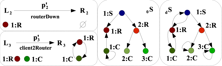
In this case there are sequences that transform state ${}_{0}S$ in ${}_{d}S$, for example, $s_{4}=p_{4};p^{\prime}_{3};p_{1};p^{\prime}_{2}$. Note that the problems are in edges $\left(1:S,1:R\right)$ and $\left(1:C,1:R\right)$ of the initial state: Router $1$ is able to receive packets from server $1$ and client $1$, but not to send them.

Next, matrices for the states and their difference are calculated. The first three columns correspond to edges (first to clients, second to routers and third to servers) and fourth to nodes which has been split by a vertical line for illustrative purposes only. The ordering of nodes is $[C\;R\;S]$ both by columns and by rows.

$${}_{0}\!S=\left[\begin{array}[]{rrrc}\vskip-6.0pt1&1&0&|\;3\\ \vskip-6.0pt2&0&0&|\;2\\ \vskip-6.0pt0&2&0&|\;1\\ \end{array}\right];\quad{}_{d}\!S=\left[\begin{array}[]{rrrc}\vskip-6.0pt2&1&0&|\;3\\ \vskip-6.0pt3&0&1&|\;2\\ \vskip-6.0pt0&2&0&|\;1\\ \end{array}\right];\quad S={}_{d}\!S-{}_{0}\!S=\left[\begin{array}[]{rrrc}\vskip-6.0pt1&0&0&|\;0\\ \vskip-6.0pt1&0&1&|\;0\\ \vskip-6.0pt0&0&0&|\;0\\ \end{array}\right]$$

The incidence tensors for every production (recall that $p_{2}$ and $p_{3}$ are as in Fig. 119) have the form

$$A^{i}_{j1}=\left[\begin{array}[]{rrrcc}\vskip-6.0pt0&0&0&|\;0&|\;C\\ \vskip-6.0pt0&0&1&|\;1&|\;R\\ \vskip-6.0pt0&1&0&|\;0&|\;S\\ \end{array}\right]\qquad A^{i}_{j2}=\left[\begin{array}[]{rrrcc}\vskip-6.0pt0&0&0&|\;\phantom{-}\phantom{,}0&|\;C\\ \vskip-6.0pt0&0&0&|\,-1&|\;R\\ \vskip-6.0pt0&0&0&|\;\phantom{-}\phantom{,}0&|\;S\\ \end{array}\right]$$

$$A^{i}_{j3}=\left[\begin{array}[]{ccccc}\vskip-6.0pt0&1&0&|\;0&|\;C\\ \vskip-6.0pt1&0&0&|\;0&|\;R\\ \vskip-6.0pt0&0&0&|\;0&|\;S\\ \end{array}\right]\quad\;\;\;A^{i}_{j4}=\left[\begin{array}[]{ccccc}\vskip-6.0pt1&0&0&|\;0&|\;C\\ \vskip-6.0pt0&0&0&|\;0&|\;R\\ \vskip-6.0pt0&0&0&|\;0&|\;S\\ \end{array}\right]$$

Although it does not seem to be strictly necessary here, more information is kept and calculations are more flexible if production $p_{4}$ is split into the part that deletes messages and the part that adds them, $p_{4}=p_{4}^{+};p_{4}^{-}$. Refer to comments in Sec. 46.

$$A^{i-}_{j4}=\left[\begin{array}[]{ccccc}\vskip-6.0pt-1&0&0&|\;0&|\;C\\ \vskip-6.0pt0&0&0&|\;0&|\;R\\ \vskip-6.0pt0&0&0&|\;0&|\;S\\ \end{array}\right]\qquad A^{i+}_{j4}=\left[\begin{array}[]{ccccc}\vskip-6.0pt2&0&0&|\;0&|\;C\\ \vskip-6.0pt0&0&0&|\;0&|\;R\\ \vskip-6.0pt0&0&0&|\;0&|\;S\\ \end{array}\right]$$

As in the example of Sec. 47, the following matrices are more appropriate for calculations:

$$A^{i}_{\!1k}\!=\!\left[\begin{array}[]{ccccc}\vskip-6.0pt0&0&0&-1&2\\ \vskip-6.0pt0&0&1&0&0\\ \vskip-6.0pt0&0&0&0&0\\ \end{array}\right]\quad A^{i}_{\!2k}\!=\!\left[\begin{array}[]{ccccc}\vskip-6.0pt0&0&1&0&0\\ \vskip-6.0pt0&0&0&0&0\\ \vskip-6.0pt1&0&0&0&0\\ \end{array}\right]$$

$$A^{i}_{\!3k}\!=\!\left[\begin{array}[]{ccccc}\vskip-6.0pt0&0&0&0&0\\ \vskip-6.0pt1&0&0&0&0\\ \vskip-6.0pt0&0&0&0&0\\ \end{array}\right]\quad A^{i}_{\!4k}\!=\!\left[\begin{array}[]{ccccc}\vskip-6.0pt0&0&0&0&0\\ \vskip-6.0pt1&-1&0&0&0\\ \vskip-6.0pt0&0&0&0&0\\ \end{array}\right]$$

If equation (274) was directly applied, we would get $x^{1}=0$ and $x^{1}=1$ (third row of $A^{i}_{\!2k}$ and second of $A^{i}_{\!3k}$) deriving a contradiction. The variations permitted for the initial state are given by the matrix

$${}_{0}\!M\mathfrak{e}=\left[\begin{array}[]{cccc}0&\alpha^{1}_{2}&0&0\\ \alpha^{2}_{1}&0&0&0\\ 0&\alpha^{3}_{2}&0&0\\ \end{array}\right]$$ (277)

with $\alpha^{1}_{2}\in\{0,-1\},\;\alpha^{2}_{1},\alpha^{3}_{2}\in\{0,-1,-2\}$. Setting $b^{1}_{2}=-1$ and $b^{3}_{2}=-1$ (one edge $\left(S,R\right)$ and one edge $\left(C,R\right)$ removed) the system to be solved is

$$\left[\begin{array}[]{cccc}1&1&0&0\\ 1&0&1&0\\ 0&1&0&0\end{array}\right]=\left[\begin{array}[]{cccc}-x^{4}+2x^{4}&\;x^{3}&0&0\\ x^{3}&0&\;x^{1}&x^{1}-x^{2}\\ 0&\;x^{1}&0&0\end{array}\right]$$

with solution $x^{1}=x^{2}=x^{3}=x^{4}=1$, $s_{4}$ being one of its associated sequences. Notice that the restriction in Prop. 48.1 is fulfilled, see equation (277). $\blacksquare$

In previous example, as we knew a sequence ($s_{4}$) answer to the reachability problem, we have fixed matrix $b$ directly to show how Prop. 48.1 works. Although this will not be normally the case, the way to proceed is very similar: Relax matrix $M$ by subtracting $b$, find a set of solutions $\{x,b\}$ and check whether the restriction for matrix $b$ is fulfilled or not.

48.2 Internal $\varepsilon$-production

Internal $\varepsilon$-productions delete edges appended or used by productions preceding it in the sequence. In this subsection we first limit to sequences which may have only internal $\varepsilon$-productions and, by the end of the section, we will put together Prop. 48.1 from Subsec. 48.1 with results derived here to state Theorem 48.3 for floating Matrix Graph Grammars.

The proposed way to proceed is analogous to that of external $\varepsilon$-productions. The idea is to allow some variation in the amount of edges erased by every production, but this variation is constrained depending on the behaviour (definition) of the rest of the rules. Unfortunately, not so much information is gathered in this case and what we are basically doing is ignoring this part of the state equation.

Define $h^{i}_{\!jk}=\left[A^{i}_{\!jk}\left(\mathfrak{e}\otimes\mathbb{I}_{k}\right)\right]^{+}=\max\left(\left\{A(\mathfrak{e}\otimes\mathbb{I}),0\right\}\right)$, where vector $\mathbb{I}_{k}=[1,\ldots,1]_{(1,k)}$.

Proposition 48.2

A necessary condition for state ${}_{d}\mathrm{M}$ to be reachable (from state ${}_{0}\mathrm{M}$) is:

$$M^{i}_{j}=\sum_{k=1}^{n}\left(A^{i}_{\!jk}+V\right)x^{k}$$ (278)

with the restriction $h^{i}_{\!jk}\leq V^{i}_{\!jk}\leq 0$.

Proof
$\square$$\blacksquare$

In some sense, external $\varepsilon$-productions are the limiting case of internal $\varepsilon$-productions and can be seen almost as a particular case: As $\varepsilon$-productions do not interfere with previous productions they have to act exclusively on the host graph.

The full generalization of the state equation for non-restricted Matrix Graph Grammars is given in the next theorem.

Theorem 48.3 (State Equation)

With notation as above, a necessary condition for state ${}_{d}\mathrm{M}$ to be reachable (from state ${}_{0}\mathrm{M}$) is

$$M^{i}_{\!j}=\sum_{k=1}^{n}\left(A^{i}_{jk}+V\right)x^{k}+b^{i}_{\!j},$$ (279)

with $b^{i}_{\!j}$ satisfying restrictions specified in Prop. 48.1 and $V$ satisfying those in Prop. 48.2.

Proof
$\square$$\blacksquare$

One interesting possibility of eq. (279) is that we can specify if productions acting on some edges must have a fixed or floating behaviour, depending whether variances are permitted or not.

Strengthening hypothesis, formula (279) becomes those already studied for floating grammars with internal $\varepsilon$-productions ($b=0$), with external $\varepsilon$-productions ($V=0$), fixed grammars (from multilinear to linear transformations) or Petri nets, fully recovering the original form of the state equation.

49 Summary and Conclusions

The starting point of the present chapter is the study of Petri nets as a particular case of Matrix Graph Grammars. We have adapted concepts of Matrix Graph Grammars to Petri nets, such as initial marking. Next, reachability and the state equation have been reformulated and extended with the language of this approach, trying to provide tools for grammars as general as possible.

Matrix Graph Grammars have also benefited from the theory developed for Petri nets: Through the generalized state equation (279) it is possible to tackle problem 4.

Despite the fact that the more general the grammar is, the less information the state equation provides, Theorem 48.3 can be considered as a full generalization of the state equation.

Equation (279) is more accurate as long as the rate of the amount of types of nodes with respect to the amount of nodes approaches one. Hence, in general, it will be of little practical use if there are many nodes but few types.

Although the use of vector spaces (as in Petri nets) and multilinear algebra is almost straightforward, many other algebraic structures are available to improve the results herein presented. For example, Lie algebras seem a good candidate if we think of the Lie bracket as a measure of commutativity (recall Subsec. 45 in which we saw that this is one of the main problems of using linear combinations).

It should be possible to extend a little the Lie bracket to consider two sequences instead of just two productions. With the theory of Chap. id1 the case of one production and one sequence can be directly addressed.

Other Petri nets concepts have algebraic characterizations and can be studied with Matrix Graph Grammars. Also, it is possible to extend their definition from Petri nets to Matrix Graph Grammars. A short summary of some of them follows:

• Conservative Petri nets are those for which the sum of the tokens remains constant. For example, think of tokens as resources of the problem under consideration.

• An invariant is some quantity that does not change during runtime. They are divided in two main families: Place invariants and transition invariants.

• Liveness studies whether transitions in a Petri net can be fired. There are five levels ($L0$ to $L4$) with algebraic characterizations of necessary conditions.

• Boundedness of a Petri net studies the number of tokens in places (in particular if this number remains bounded). Sufficient conditions are known.

Note that reachability can be directly used to study invariance under sequences of initial states. If the initial state must not change, set the initial and the final states as one and the same. This way, the state equation must be equalized to zero. This is related to termination because if there are sequences that leave some state invariant, then there are cycles in the execution of the grammar, preventing termination.

The book finishes in Chap. id1, a summary with further research proposals. Appendix id1 presents a full worked out example that illustrates all relevant concepts presented in this dissertation in a more or less realistic case. Its main objective is to show the use and practical utility of compatibility, coherence, minimal and negative initial digraphs, applicability, sequential independence and reachability. In particular properties of the system related to problems 1, 3 and 4 are addressed.

Chapter Conclusions and Further Research

This chapter closes the main body of the book. There is still Appendix A. It includes a detailed real world case study in which much of the theory developed so far is applied.

This chapter is organized in two sections. In Sec. 50 we summarize the theory and highlight some topics that can be further investigated with Matrix Graph Grammars as developed so far. Sec. 51 exposes a long term program to address termination, confluence and complexity from the point of view of Matrix Graph Grammars.

50 Summary and Short Term Research

In this book we have presented a new theory to study graph dynamics. Also, increasingly difficult problems of graph grammars have been addressed: Applicability, sequential independence and reachability.

First, two characterizations of action over graphs (known as productions or grammar rules) are defined, one emphasizing its static part and one its dynamics. To some extent it is possible to study these actions without taking into account the initial state of the system. Hence, information on the grammar can be gathered at design time, being potentially useful during runtime. Nodes and edges are considered independently, although related by compatibility. It should be possible, using the tensorial construction of Chap. id1, to define a single (algebraic) structure and set compatibility as one of its axioms (a property to be fulfilled).

Sequences of productions are studied in great detail as they are responsible for the dynamics of any grammar. Composition, parallelism and true concurrency have also been addressed.

The effect of a rule on a graph depends on where the rule is applied (matching). In Matrix Graph Grammars, matches are injective morphisms. As different productions in a sequence can be applied at different places non-deterministically, marking links parts of productions guaranteeing their applicability on the same elements. It is possible to define both matching and marking as operators acting on productions.

Production application may have side effects, e.g. the deletion of dangling edges. A special type of productions, known as $\varepsilon$-productions, appear to keep compatibility. It is shown that they are the output of some operator acting on productions as well as matching and marking. Operators for compatibility, matching and marking can be translated into productions of a sequence. This new perspective eases their analysis.

Minimal and negative initial digraphs are respectively generalized to initial and negative digraph sets. Two characterizations for applicability are given. One depends on coherence and compatibility and the other on minimal and negative initial digraphs.

Sequential independence is closely related to commutativity, but with the possibility to consider more than two elements at a time. This has been studied in the case of one production being advanced or delayed an arbitrary (but finite) number of positions.

One interesting question is whether two sequences need the same initial elements or not, especially when one is a permutation of the other. G-congruence and congruence conditions tackle this point again for one production being advanced or delayed a finite number of positions inside a sequence. An interesting topic for further study is to obtain similar results but considering moving blocks of productions instead of a single production.

Graph constraints and particularly application conditions are of great interest, mainly for two reasons: First, the left hand side and the nihilation matrix are particular cases, and second it is possible to deal with multidigraphs without any major modifications of the theory. We have seen that application conditions are a particular case of graph constraints and that a graph constraint can be reduced to an application condition in the presence of a production. Application conditions can again be seen as operators acting on productions. This, once more, means that they are equivalent to sequences of a certain type. Among other things, this reduces the study of consistency of application conditions to that of applicability.

As it is possible to transform preconditions into postconditions and back again, they are in some sense delocalized in a production. Although this is sketched in some detail in Chap. id1, no concrete theorem is established concerning the possibility to move application conditions among productions inside a sequence. We do not foresee, to the best of our knowledge, any special difficulty in addressing this topic with the theory developed so far. This would be one application of sequential independence – problem 3 – to application conditions.

Finally, in order to consider reachability – problem 4 – Petri nets are presented as a particular case of Matrix Graph Grammars. From this perspective, notions of Matrix Graphs Grammars like the minimal initial digraph are directly applied to Petri nets. Also it is interesting that concepts and results from Petri nets can be generalized to be included in Matrix Graph Grammars. Precisely, one example of this is reachability. Some other concepts can also be investigated such as liveness, boundedness, etc., and are left for future work.

For our research in reachability we have almost directly generalized previous approaches (vector spaces) to reachability by using tensor algebra. It is worth studying other algebraic structures such as Lie algebras. Also, our study of reachability has not taken into account the nihilation matrix nor application conditions, other two possible directions for further research.

In our opinion, the main contribution of this book is the novelty of the graph grammar representation, simple and powerful. It naturally brings in several branches of mathematics that can be applied to Matrix Graph Grammars, allowing a potential use of advanced results to solve old and new problems: First and second order logics, group theory, tensor algebra, graph theory, category theory and functional analysis.

51 Long Term Research Program

On the practical side, as Appendix A shows, some tasks need to be automated to ease further research. Manipulations can get rather tedious and error prone. The development or improvement of a tool such as AToM³ would be very valuable. Besides, a good behavior of an implementation of Matrix Graph Grammars is expected.

At a more theoretical level we propose to study other three increasingly difficult problems: Termination, confluence and complexity. We think that the theory developed in this book can be useful. See Fig. 120.

Figure 120: Diagram of Problem Dependencies.

Termination, in essence, asks whether there is a solution for a given problem (if some state is reached). In other branches of mathematics this is the well-known concept of existence. Reachability with some improvements can be of help in two directions. Starting in some initial state, if for some sequence of productions some invariant state is reached, then the grammar can not be terminating (as it enters a cycle as soon as it is reached). Second, to check the invariance for a given state (if there exists some sequence that leaves the graph unaltered), the state equation can also be used by equaling the initial and final states.

If we have a terminating grammar we may wonder whether there is a single final state or more than one: Confluence. In other branches of mathematics this is the well-known concept of uniqueness. Sequential independence can be used in this case.

If a grammar is terminating and confluent, the next natural question seems to be how much it takes to get to its final state. This is complexity, which can also be addressed using Matrix Graph Grammars. It is not difficult to interpret Matrix Graph Grammars as a new model of computation, just as Boolean Circuits [79] or Turing machines [58]. This is currently our main direction of research. See [67] for some initial results. The main concept addressed in this book is sequentialization, whose complexity is encoded the classes P, NP and more generally in the Polynomial Hierarchy, PH. See [58] for a comprehensive introduction to this topic.

Notice that there are two properties that make Matrix Graph Grammars differ from standard Turing machines: Its potential non-uniformity (shared with Boolean Circuits) and the use of an oracle, in its strongest version, whose associated decision problem is NP-complete.

Non-uniformity is widely addressed in the theory of Boolean Circuits. The same ideas possibly with some changes can be applied to Matrix Graph Grammars.

The strongest version of Matrix Graph Grammars as introduced here use an oracle whose associated decision problem is NP-complete: The subgraph isomorphism problem, SI, to match the left hand side of a production in the host graph. If problems that need to distinguish lower level complexity classes (assuming P$\neq$NP) such as P are considered, it is possible to restrict ourselves to some proper submodel of computation. For example, the match operation can be forced to use GI instead.

Limitations on matching are not the only natural submodels of Matrix Graph Grammars. The permitted operations can be constrained, for example forbidding the addition and deletion of nodes (this would be closely related to non-uniformity and the use of a GI-complete problem rather than SI). Also, we can act on the set of permitted graphs to derive submodels of computation. For example, consider only those graphs with a single incoming and a single outgoing edge in every node.

Chapter Case Study

This Appendix presents a full worked out example that illustrates many of the concepts and results of this book (more conceptual aspects such as functional representations, adjoints and the like are omitted in this appendix). Although the aim of Matrix Graph Grammars is to be a theoretical tool for the study of graph grammars and graph transformation systems, we will see that it is also of practical interest.

The case study herein presented tries to be simple enough to be approached with paper and pencil but complex enough to look realistic.

As will be noticed throughout this appendix, Matrix Graph Grammars (as well as any approach to graph transformation) encourages the definition of a particular language to solve a particular problem. These are known as Domain-Specific languages (DSL). See [35].

Section A presents an assembly line with four types of machines (assembler, disassembler, quality and packaging), one or more operators and some items to process. Section B presents some sequences and derivations, together with possible states of the system. Section C tackles minimal and negative initial digraphs and G-congruence. As we progress, the example will be enlarged to be more detailed. Section D deals with applicability, sequential independence, reachability and confluence. Graph constraints and application conditions are exemplified in Sec. E. Section F returns to derivations, adding and modifying productions. Dangling edges and their treatment with $\varepsilon$-productions will show up throughout the case study.

Appendix A Presentation of the Scenario

In this section our sample scenario is set up. Some basic concepts will be illustrated: Matrix representation of graphs and productions (Sec. 18), compatibility (Secs. 6, 18 and 25), completion (Sec. 19) and the nihilation matrix (Sec. 21).

Our initial assembly line will consist of four machines that take as input one or more items and output one or more items. Depending on the machine, items are processed transforming them into other items or some decision is taken (reject, accept items) with no modification.

There are four types of items, item1 – item4. One assembly machine (named assembler, connected to two input conveyors) processes one piece of item1 and one piece of item2 to output in another conveyor one piece of type item3. There is a quality assurance machine – quality – that checks if item3 fulfills certain quality standards. If it does, then item3 is accepted and packed to further produce item4 through a packaging machine. On the contrary, it is rejected and recycled through machine disassembler. Machines need the presence of an operator in order to work properly. Elements are graphically represented in Fig. 121.

Figure 121: Graphical Representation of System Actors

In this case study types are those in Fig. 121. There can be more than one element of each type, e.g there are six elements of type conveyor in Fig. 126, which shows a snapshot of the state of an example of assembly line. For typing conventions refer to comments on the example in p. 19.

Note that for now conveyors have infinite load capacity, elements in a conveyor are not ordered and one operator can simultaneously manage two or more machines. It should be desirable that one operator might look after different machines but only one at a time. This can be guaranteed only with graph constraints although if the initial state fulfills this condition and productions observe this fact, there should be no problem. We will return to this point in Sec. E.

Figure 122: DSL Syntax Specification

When dealing with DSLs, it is customary to specify its syntax through a meta-model. We will restrict connections among the different actors of the system:

• Operators can only be connected to machines (by the end of Sec. B this will be relaxed).

• Items can only be connected to conveyors (until Sec. E in which they will be allowed to be connected to other items).

• Conveyors can only be connected to machines or to other conveyors.

• Machines can be connected only to conveyors (by the end of Sec. B this will be relaxed).

These restrictions have a natural graph representation (see Fig. 122), which is sometimes referred to as typed graphs, [10]. Notice that for simplicity all actual types have been omitted. For example, there should be four nodes for the different types of items ($\mathtt{item1},\ldots,\mathtt{item4}$) and the same for the machines.

Now we describe the actions that can be performed. These are the grammar rules. The state machine will evolve according to them. See Fig. 123 for the basic productions. We will enlarge or amend them and add some others in future sections.

Figure 123: Basic Productions of the Assembly Line

Machines are not fully automatic so in this four productions one operator is needed. The four basic actions are assemble, disassemble, certify and pack. They correspond to productions assemble, recycle, certify and pack. Identifications are obvious so they have not been made explicit (numbers between different productions need not be related, i.e. 1:conv in production assem and 1:conv in certify can be differently identified in a host graph).

There are four rules that permit operators to change from one machine to another. This movement is cyclic (to make the grammar a little bit more interesting). A practical justification could be that the manager of the department obliges every operator passing near a machine to check if there is any task pending, attending it just in case. We will start with a single operator to avoid collapses. See grammar rules move2A, move2Q, move2P and move2D in Fig. 124.

Figure 124: Productions for Operator Movement

The last set of productions specify machines and operators break-down (the ’b’ in front of the productions). Fortunately for the company they can be fixed or replaced (the ’f’ in front of the productions). See Fig. 125 for the productions, where as usual $\emptyset$ stands for the empty graph. In order to save some space we have summarized four rules (one per machine) substituting the name of the machine by an $X$. This is notationally convenient but we should bear in mind that there are four rules for machines break down (bMachA, bMachQ, bMachP and bMachD) and another four for machines fixing (fMachA, fMachQ, fMachP and fMachD). Also, they can be thought of as abstract rules or variable nodes as in Sec. 43. The total amount of grammar rules up to now is twenty.

Figure 125: Break-Down and Fixing of Assembly Line Elements

Here we face the problem of $\varepsilon$-productions for the first time. If a conveyor with two items breaks (disappears) due to rule bConv, there will be at least two dangling edges, one from its input machine and another to its output machine. These dangling edges could be avoided defining one production per conveyor that takes them into account. If the conveyor had any item, then the corresponding edge would also dangle. Again this can be avoided if there is a limit in the number of pieces that a conveyor can carry, but a rule for each one is again needed. Another possibility for DPO-like graph transformation systems (what we have called fixed graph grammars) is to define a sort of subgrammar that takes care of potential dangling edges. This subgrammar productions would be applied iteratively until no edge can dangle. This is a characteristic of fixed graph transformation systems and in some situations can be a bit annoying. If there is no limit to the number of items (or the limit is too high, e.g. a memory stack in a CPU RAM), it is possible to use fixed graph grammars only to some extent. Thus, $\varepsilon$-productions are useful – at times essential – from a practical point of view, among other things, to decrease the number of productions in a grammar (this probably eases grammar definition and maintenance and increases runtime efficiency).

Matrix representation of these rules is almost straightforward according to Sec. 18. We will explicitly write the static (left and right hand sides) and dynamic representations (deletion, addition and nihilation matrices) of production assemble.

Elements are ordered [1:item1 1:item2 1:conv 2:conv 3:conv 1:macA 1:op] for $L^{E}_{\textrm{assem}}$ and $L^{N}_{\textrm{assem}}$, i.e. element $(1,3)$ of matrix $L^{E}_{\textrm{assem}}$ is the edge that starts in node (1:item1) and ends in the first conveyor, (1:conv). The ordering for productions $R^{E}_{\textrm{assem}}$ and $R^{N}_{\textrm{assem}}$ is [1:item3 1:conv 2:conv 3:conv 1:macA 1:op]. Numbers in front of types are a means to distinguish between elements of the same type in a given graph (these are the numbers that appear in Fig. 123).

$$L^{E}_{assem}\!=\!\left[\begin{array}[]{ccccccc}\vskip-6.0pt0&0&1&0&0&0&0\\ \vskip-6.0pt0&0&0&1&0&0&0\\ \vskip-6.0pt0&0&0&0&0&1&0\\ \vskip-6.0pt0&0&0&0&0&1&0\\ \vskip-6.0pt0&0&0&0&0&0&0\\ \vskip-6.0pt0&0&0&0&1&0&0\\ \vskip-6.0pt0&0&0&0&0&1&0\\ \end{array}\right],R^{E}_{assem}\!=\!\left[\begin{array}[]{cccccc}\vskip-6.0pt0&0&0&1&0&0\\ \vskip-6.0pt0&0&0&0&1&0\\ \vskip-6.0pt0&0&0&0&1&0\\ \vskip-6.0pt0&0&0&0&0&0\\ \vskip-6.0pt0&0&0&1&0&0\\ \vskip-6.0pt0&0&0&0&1&0\\ \end{array}\right],L^{N}_{assem}\!=\!\left[\begin{array}[]{c}\vskip-6.0pt1\\ \vskip-6.0pt1\\ \vskip-6.0pt1\\ \vskip-6.0pt1\\ \vskip-6.0pt1\\ \vskip-6.0pt1\\ \vskip-6.0pt1\\ \end{array}\right],R^{N}_{assem}\!=\!\left[\begin{array}[]{c}\vskip-6.0pt1\\ \vskip-6.0pt1\\ \vskip-6.0pt1\\ \vskip-6.0pt1\\ \vskip-6.0pt1\\ \vskip-6.0pt1\\ \end{array}\right].$$

For $e^{E}$, $e^{N}$, $r^{E}$ and $r^{N}$ we have the same ordering of elements.

$$e^{E}_{assem}\!=\!\left[\begin{array}[]{ccccccc}\vskip-6.0pt0&0&1&0&0&0&0\\ \vskip-6.0pt0&0&0&1&0&0&0\\ \vskip-6.0pt0&0&0&0&0&0&0\\ \vskip-6.0pt0&0&0&0&0&0&0\\ \vskip-6.0pt0&0&0&0&0&0&0\\ \vskip-6.0pt0&0&0&0&0&0&0\\ \vskip-6.0pt0&0&0&0&0&0&0\\ \end{array}\right],r^{E}_{assem}\!=\!\left[\begin{array}[]{cccccc}\vskip-6.0pt0&0&0&1&0&0\\ \vskip-6.0pt0&0&0&0&0&0\\ \vskip-6.0pt0&0&0&0&0&0\\ \vskip-6.0pt0&0&0&0&0&0\\ \vskip-6.0pt0&0&0&0&0&0\\ \vskip-6.0pt0&0&0&0&0&0\\ \end{array}\right],e^{N}_{assem}\!=\!\left[\begin{array}[]{c}\vskip-6.0pt1\\ \vskip-6.0pt1\\ \vskip-6.0pt0\\ \vskip-6.0pt0\\ \vskip-6.0pt0\\ \vskip-6.0pt0\\ \vskip-6.0pt0\\ \end{array}\right],r^{N}_{assem}\!=\!\left[\begin{array}[]{c}\vskip-6.0pt1\\ \vskip-6.0pt0\\ \vskip-6.0pt0\\ \vskip-6.0pt0\\ \vskip-6.0pt0\\ \vskip-6.0pt0\\ \end{array}\right].$$

The production is defined $R=p(L)=r\vee\overline{e}L$ both for edges and for nodes. To operate it is mandatory to complete the matrices. See equation (281) for the implicit ordering of elements.

$$\underbrace{\left[\begin{array}[]{cccccccc}\vskip-6.0pt0&0&0&0&0&0&0&0\\ \vskip-6.0pt0&0&0&0&0&0&0&0\\ \vskip-6.0pt0&0&0&0&0&1&0&0\\ \vskip-6.0pt0&0&0&0&0&0&1&0\\ \vskip-6.0pt0&0&0&0&0&0&1&0\\ \vskip-6.0pt0&0&0&0&0&0&0&0\\ \vskip-6.0pt0&0&0&0&0&1&0&0\\ \vskip-6.0pt0&0&0&0&0&0&1&0\\ \end{array}\right]}_{R^{E}_{assem}}=\underbrace{\left[\begin{array}[]{cccccccc}\vskip-6.0pt0&0&0&0&0&0&0&0\\ \vskip-6.0pt0&0&0&0&0&0&0&0\\ \vskip-6.0pt0&0&0&0&0&1&0&0\\ \vskip-6.0pt0&0&0&0&0&0&0&0\\ \vskip-6.0pt0&0&0&0&0&0&0&0\\ \vskip-6.0pt0&0&0&0&0&0&0&0\\ \vskip-6.0pt0&0&0&0&0&0&0&0\\ \vskip-6.0pt0&0&0&0&0&0&0&0\\ \end{array}\right]}_{r^{E}_{assem}}\vee\underbrace{\overline{\left[\begin{array}[]{cccccccc}\vskip-6.0pt0&0&0&1&0&0&0&0\\ \vskip-6.0pt0&0&0&0&1&0&0&0\\ \vskip-6.0pt0&0&0&0&0&0&0&0\\ \vskip-6.0pt0&0&0&0&0&0&0&0\\ \vskip-6.0pt0&0&0&0&0&0&0&0\\ \vskip-6.0pt0&0&0&0&0&0&0&0\\ \vskip-6.0pt0&0&0&0&0&0&0&0\\ \vskip-6.0pt0&0&0&0&0&0&0&0\\ \end{array}\right]}}_{\overline{e^{E}_{assem}}}\underbrace{\left[\begin{array}[]{cccccccc}\vskip-6.0pt0&0&0&1&0&0&0&0\\ \vskip-6.0pt0&0&0&0&1&0&0&0\\ \vskip-6.0pt0&0&0&0&0&0&0&0\\ \vskip-6.0pt0&0&0&0&0&0&1&0\\ \vskip-6.0pt0&0&0&0&0&0&1&0\\ \vskip-6.0pt0&0&0&0&0&0&0&0\\ \vskip-6.0pt0&0&0&0&0&1&0&0\\ \vskip-6.0pt0&0&0&0&0&0&1&0\\ \end{array}\right]}_{L^{E}_{assem}}$$ (280)

The expression for nodes is similar. As pointed out in Sec. 44, using a similar construction to that of Sec. 47 (in the definition of the incidence tensor 47.3) it should be possible to get a single expression for both nodes and edges instead of a formula for edges and a formula for nodes. This might be of interest for implementations of Matrix Graph Grammars as more compact expressions would be derived.

We shall mainly concentrate on edges because they define matrices instead of just vectors and all problems such as inconsistencies (dangling elements) come this way.

$$\underbrace{\left[\begin{array}[]{cl}\vskip-6.0pt0&|\;\textrm{{1:item1}}\\ \vskip-6.0pt0&|\;\textrm{{1:item2}}\\ \vskip-6.0pt1&|\;\textrm{{1:item3}}\\ \vskip-6.0pt1&|\;\textrm{{1:conv}}\\ \vskip-6.0pt1&|\;\textrm{{2:conv}}\\ \vskip-6.0pt1&|\;\textrm{{3:conv}}\\ \vskip-6.0pt1&|\;\textrm{{1:machA}}\\ \vskip-6.0pt1&|\;\textrm{{1:op}}\\ \end{array}\right]}_{R^{N}_{assem}}=\underbrace{\left[\begin{array}[]{cl}\vskip-6.0pt0&|\;\textrm{{1:item1}}\\ \vskip-6.0pt0&|\;\textrm{{1:item2}}\\ \vskip-6.0pt1&|\;\textrm{{1:item3}}\\ \vskip-6.0pt0&|\;\textrm{{1:conv}}\\ \vskip-6.0pt0&|\;\textrm{{2:conv}}\\ \vskip-6.0pt0&|\;\textrm{{3:conv}}\\ \vskip-6.0pt0&|\;\textrm{{1:machA}}\\ \vskip-6.0pt0&|\;\textrm{{1:op}}\\ \end{array}\right]}_{r^{N}_{assem}}\vee\underbrace{\overline{\left[\begin{array}[]{cl}\vskip-6.0pt1&|\;\textrm{{1:item1}}\\ \vskip-6.0pt1&|\;\textrm{{1:item2}}\\ \vskip-6.0pt0&|\;\textrm{{1:item3}}\\ \vskip-6.0pt0&|\;\textrm{{1:conv}}\\ \vskip-6.0pt0&|\;\textrm{{2:conv}}\\ \vskip-6.0pt0&|\;\textrm{{3:conv}}\\ \vskip-6.0pt0&|\;\textrm{{1:machA}}\\ \vskip-6.0pt0&|\;\textrm{{1:op}}\\ \end{array}\right]}}_{\overline{e^{N}_{assem}}}\underbrace{\left[\begin{array}[]{cl}\vskip-6.0pt1&|\;\textrm{{1:item1}}\\ \vskip-6.0pt1&|\;\textrm{{1:item2}}\\ \vskip-6.0pt0&|\;\textrm{{1:item3}}\\ \vskip-6.0pt1&|\;\textrm{{1:conv}}\\ \vskip-6.0pt1&|\;\textrm{{2:conv}}\\ \vskip-6.0pt1&|\;\textrm{{3:conv}}\\ \vskip-6.0pt1&|\;\textrm{{1:machA}}\\ \vskip-6.0pt1&|\;\textrm{{1:op}}\\ \end{array}\right]}_{L^{N}_{assem}}$$ (281)

Note that some elements in the node vectors are zero. This means that these nodes appear in the algebraic expressions but are not part of the graphs.

The nihilation matrix in this case includes all edges incident to any node that is deleted plus edges that are added by production assem. See Lemma 21.2 for its calculation formula:

$$K_{\textrm{{assem}}}=\left[\begin{array}[]{ccccccccl}\vskip-6.0pt1&1&1&0&1&1&1&1&|\;\textrm{{1:item1}}\\ \vskip-6.0pt1&1&1&1&0&1&1&1&|\;\textrm{{1:item2}}\\ \vskip-6.0pt1&1&0&0&0&1&0&0&|\;\textrm{{1:item3}}\\ \vskip-6.0pt1&1&0&0&0&0&0&0&|\;\textrm{{1:conv}}\\ \vskip-6.0pt1&1&0&0&0&0&0&0&|\;\textrm{{2:conv}}\\ \vskip-6.0pt1&1&0&0&0&0&0&0&|\;\textrm{{3:conv}}\\ \vskip-6.0pt1&1&0&0&0&0&0&0&|\;\textrm{{1:machA}}\\ \vskip-6.0pt1&1&0&0&0&0&0&0&|\;\textrm{{1:op}}\\ \end{array}\right]$$ (282)

Let’s consider sequence bOp;assem to see how formula (4) works to check compatibility (Props. 6.4 and 18.6). We can foresee a problem with edge (1:op,1:machA) because the node disappears but not the edge.

According to eq. (148) we need to check compatibility for the increasing set of sequences s1 = assem and s2 = bOp;assem. Note that the minimal initial digraph is the same for both sequences and coincides with the left hand side of assem. Sequence assem is compatible, as the output of production assem is a simple digraph again, i.e. rule assemble is well defined:

$$\left\|\left[s_{1}\left(M_{\textrm{{assem}}}^{E}\right)\right.\right. \!\vee \!\left.\left.\left(s_{1}\left(M_{\textrm{{assem}}}^{E}\right)\right)^{t}\right]\odot\overline{s_{1}\left(M_{\textrm{{assem}}}^{N}\right)}\right\|_{1}=\left\|\left[R_{\textrm{{assem}}}^{E}\vee\left(R_{\textrm{{assem}}}^{E}\right)^{t}\right]\odot\overline{R_{\textrm{{assem}}}^{N}}\right\|_{1}=$$

$$= \left\|\left(\left[\begin{array}[]{cccccccc}\vskip-6.0pt0&0&0&0&0&0&0&0\\ \vskip-6.0pt0&0&0&0&0&0&0&0\\ \vskip-6.0pt0&0&0&0&0&1&0&0\\ \vskip-6.0pt0&0&0&0&0&0&1&0\\ \vskip-6.0pt0&0&0&0&0&0&1&0\\ \vskip-6.0pt0&0&0&0&0&0&0&0\\ \vskip-6.0pt0&0&0&0&0&1&0&0\\ \vskip-6.0pt0&0&0&0&0&0&1&0\\ \end{array}\right]\vee\left[\begin{array}[]{cccccccc}\vskip-6.0pt0&0&0&0&0&0&0&0\\ \vskip-6.0pt0&0&0&0&0&0&0&0\\ \vskip-6.0pt0&0&0&0&0&0&0&0\\ \vskip-6.0pt0&0&0&0&0&0&0&0\\ \vskip-6.0pt0&0&0&0&0&0&0&0\\ \vskip-6.0pt0&0&1&0&0&0&1&0\\ \vskip-6.0pt0&0&0&1&1&0&0&1\\ \vskip-6.0pt0&0&0&0&0&0&0&0\\ \end{array}\right]\right)\odot\left[\begin{array}[]{c}\vskip-6.0pt1\\ \vskip-6.0pt1\\ \vskip-6.0pt0\\ \vskip-6.0pt0\\ \vskip-6.0pt0\\ \vskip-6.0pt0\\ \vskip-6.0pt0\\ \vskip-6.0pt0\\ \end{array}\right]\right\|_{1}=0$$

Thus, there is no problem with $s_{1}$. Let’s check $s_{2}$ out. Operations are also easy for it. Note that $r_{\texttt{bOp}}\vee\overline{e}_{\texttt{bOp}}\left(R^{E}_{\texttt{assem}}\right)=R^{E}_{\texttt{assem}}$, so:

$$\left\|\left[s_{2}\left(M^{E}\right)\right.\right. \!\vee \!\left.\left.\left(s_{2}\left(M^{E}\right)\right)^{t}\right]\odot\overline{s_{1}\left(M^{N}\right)}\right\|_{1}=\left\|\left[\texttt{bOp}\left(R^{E}\right)\vee\left(\texttt{bOp}\left(R^{E}\right)\right)^{t}\right]\odot\overline{\textrm{{bOp}}\left(R^{N}\right)}\right\|_{1}$$

$$= \left\|\left[R^{E}\vee\left(R^{E}\right)^{t}\right]\odot\overline{\texttt{bOp}\left(R^{N}\right)}\right\|_{1}=\left\|\left[\begin{array}[]{cccccccc}\vskip-6.0pt0&0&0&0&0&0&0&0\\ \vskip-6.0pt0&0&0&0&0&0&0&0\\ \vskip-6.0pt0&0&0&0&0&1&0&0\\ \vskip-6.0pt0&0&0&0&0&0&1&0\\ \vskip-6.0pt0&0&0&0&0&0&1&0\\ \vskip-6.0pt0&0&1&0&0&0&1&0\\ \vskip-6.0pt0&0&0&1&1&1&0&\mathbf{1}\\ \vskip-6.0pt0&0&0&0&0&0&1&0\\ \end{array}\right]\odot\left[\begin{array}[]{c}\vskip-6.0pt1\\ \vskip-6.0pt1\\ \vskip-6.0pt0\\ \vskip-6.0pt0\\ \vskip-6.0pt0\\ \vskip-6.0pt0\\ \vskip-6.0pt0\\ \vskip-6.0pt1\\ \end{array}\right]\right\|_{1}=1$$

This kind of formulas do not only assert compatibility for the sequence, but also tells us which elements are problematic. In previous equation we see that the final answer is 1 because of element in position $(7,8)$ (bold).

In our case study as defined up to now, compatibility can only be ruined by productions starting with a ’b’ (bOp, etcetera). Either an $\varepsilon$-production is appended or the result is not a simple digraph (not a graph, actually). Some information about compatibility can be gathered at design time, on the basis of required elements appearing on the left hand side of the productions, or elements added. For example, according to productions considered so far any operator is connected to some machine so if production bOp is applied it is very likely that some dangling edge will appear. Nihilation matrices can be automatically calculated as well as completion of rules with respect to each other.

A typical snapshot of the evolution of our assembly line can be found in Fig. 126. It will be used in future sections as initial state.

Figure 126: Snapshot of the Assembly Line

Appendix B Sequences

One topic not addressed in this book is how rules in a graph grammar are selected for its application to an actual host graph. There are several possibilities. To simplify the exposition rules will be chosen randomly. As commented in Secs. 27 and 43, this is the first – out of two – source of non-determinism in graph transformation systems, in particular in Matrix Graph Grammars.

We will add another rule – reject – that discards one element once it has been assembled. It is represented in Fig. 127.

Figure 127: Graph Grammar Rule reject

We have two comments on this rule. First, reject does not need the presence of an operator to act, but it may also be applied if an operator is on the machine. Second, if grammar rules are applied randomly following some probability distribution, elements will be rejected according to the selected probability measure.

Let’s begin with one sequence that starts with one piece of type item1 and one of type item2 and produces one of type item4:

$$\texttt{s}_{\texttt{0}}=\texttt{pack;certify;assem}$$ (330)

which is compatible as no production generates any dangling edge. Recall that compatibility also depends on the host graph: If item1 was connected to two different conveyors (should this make any sense) then rule assem would produce one dangling edge.

Figure 128: Minimal Initial Digraph and Image of Sequence $\texttt{s}_{\texttt{0}}$

The minimal initial digraph of $\texttt{s}_{\texttt{0}}$ can be calculated using eq. (88)), $M_{\texttt{s}_{\texttt{0}}}=\nabla_{1}^{3}\left(\overline{r_{x}}L_{y}\right)$, where order of nodes is [1:item1 1:item2 1:item3 1:item4 1:conv 2:conv 3:conv 4:conv 5:conv 1:machA 1:machQ 1:machP 1:op]. The completion we have performed identifies operators in the productions as being the same. Also, element 1:conv in rule certify (Fig. 123) becomes 3:conv and 2:conv is now 4:conv. Similar manipulations have been performed for pack. Theorem 23.2 demands coherence in order to apply eq. (88), which is checked out in (333). More attention will be paid to initial digraphs in the next section.

$$M_{\texttt{s}_{\texttt{0}}}=L_{\texttt{assem}}\vee\overline{r}_{\texttt{assem}}L_{\texttt{certify}}\vee\overline{r}_{\texttt{assem}}\overline{r}_{\texttt{certify}}L_{\texttt{pack}}=\left[\begin{array}[]{ccccccccccccc}\vskip-6.0pt0&0&0&0&1&0&0&0&0&0&0&0&0\\ \vskip-6.0pt0&0&0&0&0&1&0&0&0&0&0&0&0\\ \vskip-6.0pt0&0&0&0&0&0&0&0&0&0&0&0&0\\ \vskip-6.0pt0&0&0&0&0&0&0&0&0&0&0&1&0\\ \vskip-6.0pt0&0&0&0&0&0&0&0&0&1&0&0&0\\ \vskip-6.0pt0&0&0&0&0&0&0&0&0&1&0&0&0\\ \vskip-6.0pt0&0&0&0&0&0&0&0&0&0&0&0&0\\ \vskip-6.0pt0&0&0&0&0&0&0&0&0&0&0&1&0\\ \vskip-6.0pt0&0&0&0&0&0&0&0&0&0&0&0&0\\ \vskip-6.0pt0&0&0&0&0&0&0&1&0&0&0&0&0\\ \vskip-6.0pt0&0&0&0&0&0&0&0&0&0&0&0&0\\ \vskip-6.0pt0&0&0&0&0&0&0&1&1&0&0&0&0\\ \vskip-6.0pt0&0&0&0&0&0&0&0&0&1&1&1&0\\ \end{array}\right]$$ (331)

The negative initial digraph is calculated using eq. (145), $K(\texttt{s}_{\texttt{0}})=\nabla_{1}^{3}\left(\overline{e}_{x}K_{y}\right)$. It is not shown in any figure because it has many edges. In order to calculate $K(\texttt{s}_{\texttt{0}})$, the nihilation matrices of productions assem (282), certify and pack are needed. Equation (79), $K=p\left(\overline{D}\right)$, can be used with the same ordering of nodes as for $M_{\texttt{s}_{\texttt{0}}}$.

$$K(\texttt{s}_{\texttt{0}})=K_{\texttt{assem}}\vee\overline{e}_{\texttt{assem}}K_{\texttt{cert}}\vee\overline{e}_{\texttt{assem}}\overline{e}_{\texttt{cert}}K_{\texttt{pack}}=\left[\begin{array}[]{ccccccccccccc}\vskip-6.0pt1&1&1&1&0&1&1&1&1&1&1&1&1\\ \vskip-6.0pt1&1&1&1&1&0&1&1&1&1&1&1&1\\ \vskip-6.0pt1&1&1&1&1&1&0&1&1&1&1&1&1\\ \vskip-6.0pt0&0&0&0&0&0&0&1&0&0&0&0&0\\ \vskip-6.0pt1&1&1&0&0&0&0&0&0&0&0&0&0\\ \vskip-6.0pt1&1&1&0&0&0&0&0&0&0&0&0&0\\ \vskip-6.0pt1&1&1&0&0&0&0&0&0&0&0&0&0\\ \vskip-6.0pt1&1&1&0&0&0&0&0&0&0&0&0&0\\ \vskip-6.0pt1&1&1&0&0&0&0&0&0&0&0&0&0\\ \vskip-6.0pt1&1&1&0&0&0&0&0&0&0&0&0&0\\ \vskip-6.0pt1&1&1&0&0&0&0&0&0&0&0&0&0\\ \vskip-6.0pt1&1&1&0&0&0&0&0&0&0&0&0&0\\ \vskip-6.0pt1&1&1&0&0&0&0&0&0&0&0&0&0\\ \end{array}\right]$$ (332)

The result of applying $\texttt{s}_{\texttt{0}}$ to $M_{\texttt{s}_{\texttt{0}}}$ is given by eq. (141), $\texttt{s}_{\texttt{0}}\left(M^{E}_{\texttt{s}_{\texttt{0}}}\right)=\bigwedge_{i=1}^{3}\left(\overline{e^{E}_{i}}M^{E}_{\texttt{s}_{\texttt{0}}}\right)\vee\bigtriangleup_{1}^{3}\left(\overline{e^{E}_{x}}\,r^{E}_{y}\right)$ and can be found to the right of Fig. 128. For its calculation, it is possible to interpret $\texttt{s}_{\texttt{0}}$ as a production according to the remark that appears right after eq. (141).

Sequence $\texttt{s}_{\texttt{0}}$ is coherent with respect to the identifications proposed in its minimal initial digraph (Fig. 128). To see this (73) in Theorem 20.5 can be used, which once simplified is eq. (69):

$$L_{\texttt{cert}}e_{\texttt{assem}} \vee L_{\texttt{pack}}\left(e_{\texttt{assem}}\,\overline{r}_{\texttt{cert}}\vee e_{\texttt{cert}}\right)\vee$$ (333)

$$\vee R_{\texttt{assem}}\left(\overline{e}_{\texttt{cert}}r_{\texttt{pack}}\vee r_{\texttt{cert}}\right)\vee R_{\texttt{cert}}r_{\texttt{pack}}=0.$$

A very simple non-coherent sequence – assuming that both rules act on the same elements – is $\texttt{t}_{\texttt{0}}=\texttt{reject};\texttt{certify}$. It is obvious as both consume the same item. When its coherence is calculated, not only will we be informed that coherence fails but also what elements are responsible for this failure.

Proposition 25.4 tells us that the rules in $\texttt{s}_{\texttt{0}}$ can be composed if they are coherent and compatible. Let $c_{0}=\left(L_{c},e_{c},r_{c}\right)$ be the rule so defined. Using equations (151) and (152) its matrices can be found. Also, taking advantage of previous calculations for the image and using Corollary 23.3, we can see that the composition is the one given in Fig. 129, closely related to Fig. 128.

Figure 129: Composition of Sequence $\texttt{s}_{\texttt{0}}$

Let $\texttt{mv}_{\texttt{1}}=\texttt{move2A};\texttt{move2D}$ and $\texttt{mv}_{\texttt{2}}=\texttt{move2P};\texttt{move2Q}$ and define the sequence $s_{4}=\texttt{pack};\texttt{mv}_{\texttt{2}};\texttt{assem};\texttt{mv}_{\texttt{1}}$. Production pack is not sequentially independent of $\texttt{mv}_{\texttt{1}}$ nor of $\texttt{mv}_{\texttt{2}};\texttt{assem}$. This is a simple example in which it is possible to advance productions inside sequences only if jumps of length strictly greater than one are allowed. To see that $\texttt{pack}\,\bot\left(\texttt{mv}_{\texttt{2}};\texttt{assem}\,;\texttt{mv}_{\texttt{1}}\right)$ it is necessary – see Theorem 33.2 – to check coherence of both sequences and G-congruence.

Coherence for advancement of a single production inside a sequence is given by eq. (200) in Theorem 33.3, which should be zero. It is straightforward to check that:

$$e_{\texttt{pack}}\bigtriangledown_{1}^{5}\left(\overline{r_{x}}\,L_{y}\right)\vee R_{\texttt{pack}}\bigtriangledown_{1}^{5}\left(\overline{e_{x}}\,r_{y}\right)=0.$$ (334)

Figure 130: DSL Syntax Specification Extended

By increasing the number of productions the system can be modelled in greater detail. For example, one operator can be busy or idle. The operator is busy if some action needs his attention. This will be represented by a self loop attached to the operator under consideration. The same applies to a machine. The syntax as a DSL of our grammar changes because there can exist self-loops for machines and operators. This is not allowed in Fig. 122. However, negative conditions are needed in the type graph (there can be self-loops in machines or operators but not connections between two operators or between two machines). See Fig. 130. We need to demand $A_{1}$ for every single edge (using the decomposition operator $\widehat{T}$ of Sec. 39) and the nonexistence of matchings with $A_{2}$ and $A_{3}$.

Up to now a single operator could be in charge of more than one machine so if there are edges from the operator to several machines, all machines may work simultaneously. Besides, there can be more than one operator working on the same machine. In a probably more realistic grammar, these two scenarios could not take place. These restrictions will be addressed in Sec. E.

Figure 131: Production assemble in Greater Detail

The production process of any machine can be split into two phases: If there are enough elements to start its job, then the input pieces disappear and the machine and the operator become busy. After that, some output piece is produced and the machine and the operator become idle again. This is represented in the sequence of Fig. 131. Note that $\texttt{assemble}=\texttt{assemble}_{\texttt{1}}\circ\texttt{assemble}_{\texttt{2}}$.

If we limit our Matrix Graph Grammar to deal with simple digraphs we have a built-in application condition “for free”. Even though one operator can still be in charge of several machines simultaneously, he will manage at most one machine at a time. Otherwise, two self-loops would be added violating compatibility.

Application conditions are needed if we want to set restrictions on productions move. This can be permitted if the machine has a kind of “pause”, so the machine (which is busy as it has a self loop) can resume as soon as an operator moves to it. It is not necessary to specify a restriction to state that a machine can not start a job when the operator is busy, as the rule would try to append a second self-loop to the operator (something not allowed if we are limited to simple digraphs).

Sequences can be generated at design time to debug the grammar or during runtime to force a set of events. They can also be automatically generated by application conditions or can be associated to other concepts, such as reachability.

Appendix C Initial Digraph Sets and G-Congruence

To calculate the initial digraph set of sequence $\texttt{s}_{\texttt{0}}=\texttt{pack}\,;\texttt{certify}\,;\texttt{assem}$ we start with the maximal initial digraph $M_{0}$, the digraph that unrelates all elements for different productions. It is formed by the disjoint union of the left hand sides of the three productions in sequence $\texttt{s}_{\texttt{0}}$. The rest of elements $M_{i}$ of the initial digraph set $\mathfrak{M}\left(s_{0}\right)$ are derived by identifying nodes and edges in $M_{0}$. These identifications however can not be carried out arbitrarily because any $M_{i}\in\mathfrak{M}\left(s_{0}\right)$ must satisfy eq. (88). Hence, there are identifications that make some elements unnecessary. For example, if the output conveyor of production certify is identified with the input conveyor of pack, then item3 (mandatory for the application of pack) is not needed anymore because it will be provided by certify.

Figure 132: MID and Excerpt of the Initial Digraph Set of $\texttt{s}_{\texttt{0}}=\texttt{pack}\,;\texttt{certify}\,;\texttt{assem}$

For $s_{0}$ we will label $c1$ and $c2$ the input conveyors of assemble and $c3$ its output conveyor. Similarly, we have $c4$ and $c5$ for certify and $c6$ and $c7$ for pack. Operators will be labelled accordingly so $o1$ is the one in assemble, $o2$ in certify and $o3$ in pack. There are two machines for packing, $m1$ the one in certify and $m_{2}$ in pack. See the graph to the left of Fig. 133. No identification prevents any other in $\mathfrak{M}\left(s_{0}\right)$, so the number of elements in $\mathfrak{M}\left(s_{0}\right)$ grows factorially. In this case, since there are 6 possible identifications we have 720 possibilities. In Fig. 132 a part of the initial digraph set can be found to the right. The string that appears close to each arrow specifies the identification (top-bottom) performed to derive the corresponding initial digraph.

Initial digraph sets can be useful to debug a grammar. By choosing certain testing sequences it is possible to automatically select “extreme” cases in which as many elements as possible are identified or unrelated. For example, the development framework can tell that a single operator may manage all machines with the grammar as defined so far, but maybe this was not the intended behavior.

Figure 133: MID for Sequences $\texttt{s}_{\texttt{1}}$ and $\texttt{s}_{\texttt{2}}$

G-congruence and congruence conditions guarantee the sameness of the minimal initial digraph. They also provide information on what elements are spoiling this property. Consider the sequences $\texttt{s}_{\texttt{1}}=\texttt{reject}\,;\texttt{assemble}\,;\texttt{recycle}$ and $\texttt{s}_{\texttt{2}}=\texttt{assemble}\,;\texttt{recycle}\,;$ reject, where in $\texttt{s}_{\texttt{2}}$ the application of production reject has been advanced two positions with respect to $\texttt{s}_{\texttt{1}}$. The minimal initial digraphs of both sequences can be found in Fig. 133. By the way, notice that $M(s_{i})$ are invariants for these transformations, i.e. $s_{i}\left(M\left(s_{i}\right)\right)=M\left(s_{i}\right)$.

G-congruence is characterized in terms of congruence conditions in Theorem 32.6. Congruence conditions for the advancement of a single production inside a sequence are stated in Prop. 32.2, in particular in eq. (192). Simplified and adapted for this case with nodes ordered [1:item1 1:item2 1:item3 1:conv 2:conv 3:conv 4:conv 1:macA 1:macQ 1:macD 1:op]:

$$CC = L_{3}\nabla_{1}^{2}\overline{e}_{x}K_{y}\left(r_{y}\vee e_{3}\right)\vee K_{3}\nabla_{1}^{2}\overline{r}_{x}L_{y}\left(e_{y}\vee r_{3}\right)=$$

$$= L_{3}\left[K_{1}\left(r_{1}\vee e_{3}\right)\vee\overline{e}_{1}K_{2}\left(r_{2}\vee e_{3}\right)\right]\vee K_{3}\left[L_{1}\left(e_{1}\vee r_{3}\right)\vee\overline{r}_{1}L_{2}\left(e_{2}\vee r_{3}\right)\right]=$$

$$= \left[\begin{array}[]{ccccccccccc}\vskip-6.0pt0&0&0&0&0&0&0&0&0&0&0\\ \vskip-6.0pt0&0&0&0&0&0&0&0&0&0&0\\ \vskip-6.0pt0&0&0&0&0&0&1&0&0&0&0\\ \vskip-6.0pt0&0&0&0&0&0&0&0&0&0&0\\ \vskip-6.0pt0&0&0&0&0&0&0&0&0&0&0\\ \vskip-6.0pt0&0&0&0&0&0&0&0&0&1&0\\ \vskip-6.0pt0&0&0&0&0&0&0&0&1&0&0\\ \vskip-6.0pt0&0&0&0&0&0&0&0&0&0&0\\ \vskip-6.0pt0&0&0&0&0&1&0&0&0&0&0\\ \vskip-6.0pt0&0&0&0&0&0&0&0&0&0&0\\ \vskip-6.0pt0&0&0&0&0&0&0&0&0&0&0\\ \end{array}\right]\left[\left[\begin{array}[]{ccccccccccc}\vskip-6.0pt0&0&1&1&0&0&0&0&0&0&0\\ \vskip-6.0pt0&0&1&0&1&0&0&0&0&0&0\\ \vskip-6.0pt1&1&1&1&1&0&1&1&1&1&1\\ \vskip-6.0pt0&0&1&0&0&0&0&0&0&0&0\\ \vskip-6.0pt0&0&1&0&0&0&0&0&0&0&0\\ \vskip-6.0pt0&0&1&0&0&0&0&0&0&0&0\\ \vskip-6.0pt0&0&1&0&0&0&0&0&0&0&0\\ \vskip-6.0pt0&0&1&0&0&0&0&0&0&0&0\\ \vskip-6.0pt0&0&1&0&0&0&0&0&0&0&0\\ \vskip-6.0pt0&0&1&0&0&0&0&0&0&0&0\\ \vskip-6.0pt0&0&1&0&0&0&0&0&0&0&0\\ \end{array}\right]\left(\left[\begin{array}[]{ccccccccccc}\vskip-6.0pt0&0&0&1&0&0&0&0&0&0&0\\ \vskip-6.0pt0&0&0&0&1&0&0&0&0&0&0\\ \vskip-6.0pt0&0&0&0&0&0&0&0&0&0&0\\ \vskip-6.0pt0&0&0&0&0&0&0&0&0&0&0\\ \vskip-6.0pt0&0&0&0&0&0&0&0&0&0&0\\ \vskip-6.0pt0&0&0&0&0&0&0&0&0&0&0\\ \vskip-6.0pt0&0&0&0&0&0&0&0&0&0&0\\ \vskip-6.0pt0&0&0&0&0&0&0&0&0&0&0\\ \vskip-6.0pt0&0&0&0&0&0&0&0&0&0&0\\ \vskip-6.0pt0&0&0&0&0&0&0&0&0&0&0\\ \vskip-6.0pt0&0&0&0&0&0&0&0&0&0&0\\ \end{array}\right]\vee\right.\right.$$

$$\vee \left.\left[\begin{array}[]{ccccccccccc}\vskip-6.0pt0&0&0&0&0&0&0&0&0&0&0\\ \vskip-6.0pt0&0&0&0&0&0&0&0&0&0&0\\ \vskip-6.0pt0&0&0&0&0&0&1&0&0&0&0\\ \vskip-6.0pt0&0&0&0&0&0&0&0&0&0&0\\ \vskip-6.0pt0&0&0&0&0&0&0&0&0&0&0\\ \vskip-6.0pt0&0&0&0&0&0&0&0&0&0&0\\ \vskip-6.0pt0&0&0&0&0&0&0&0&0&0&0\\ \vskip-6.0pt0&0&0&0&0&0&0&0&0&0&0\\ \vskip-6.0pt0&0&0&0&0&0&0&0&0&0&0\\ \vskip-6.0pt0&0&0&0&0&0&0&0&0&0&0\\ \vskip-6.0pt0&0&0&0&0&0&0&0&0&0&0\\ \end{array}\right]\right)\vee\left[\begin{array}[]{ccccccccccc}\vskip-6.0pt1&1&1&1&1&1&1&1&1&1&1\\ \vskip-6.0pt1&1&1&1&1&1&1&1&1&1&1\\ \vskip-6.0pt1&1&1&1&1&0&1&1&1&1&1\\ \vskip-6.0pt1&1&1&1&1&1&1&1&1&1&1\\ \vskip-6.0pt1&1&1&1&1&1&1&1&1&1&1\\ \vskip-6.0pt1&1&1&1&1&1&1&1&1&1&1\\ \vskip-6.0pt1&1&1&1&1&1&1&1&1&1&1\\ \vskip-6.0pt1&1&1&1&1&1&1&1&1&1&1\\ \vskip-6.0pt1&1&1&1&1&1&1&1&1&1&1\\ \vskip-6.0pt1&1&1&1&1&1&1&1&1&1&1\\ \vskip-6.0pt1&1&1&1&1&1&1&1&1&1&1\\ \end{array}\right]\left[\begin{array}[]{ccccccccccc}\vskip-6.0pt1&1&1&0&1&1&1&1&1&1&1\\ \vskip-6.0pt1&1&1&1&0&1&1&1&1&1&1\\ \vskip-6.0pt1&1&0&0&0&0&1&0&0&0&0\\ \vskip-6.0pt1&1&0&0&0&0&0&0&0&0&0\\ \vskip-6.0pt1&1&0&0&0&0&0&0&0&0&0\\ \vskip-6.0pt1&1&0&0&0&0&0&0&0&0&0\\ \vskip-6.0pt1&1&0&0&0&0&0&0&0&0&0\\ \vskip-6.0pt1&1&0&0&0&0&0&0&0&0&0\\ \vskip-6.0pt1&1&0&0&0&0&0&0&0&0&0\\ \vskip-6.0pt1&1&0&0&0&0&0&0&0&0&0\\ \vskip-6.0pt1&1&0&0&0&0&0&0&0&0&0\\ \end{array}\right]$$

$$\left.\left(\left[\begin{array}[]{ccccccccccc}\vskip-6.0pt0&0&0&0&0&0&0&0&0&0&0\\ \vskip-6.0pt0&0&0&0&0&0&0&0&0&0&0\\ \vskip-6.0pt0&0&0&0&0&0&1&0&0&0&0\\ \vskip-6.0pt0&0&0&0&0&0&0&0&0&0&0\\ \vskip-6.0pt0&0&0&0&0&0&0&0&0&0&0\\ \vskip-6.0pt0&0&0&0&0&0&0&0&0&0&0\\ \vskip-6.0pt0&0&0&0&0&0&0&0&0&0&0\\ \vskip-6.0pt0&0&0&0&0&0&0&0&0&0&0\\ \vskip-6.0pt0&0&0&0&0&0&0&0&0&0&0\\ \vskip-6.0pt0&0&0&0&0&0&0&0&0&0&0\\ \vskip-6.0pt0&0&0&0&0&0&0&0&0&0&0\\ \end{array}\right]\vee\left[\begin{array}[]{ccccccccccc}\vskip-6.0pt0&0&0&0&0&0&0&0&0&0&0\\ \vskip-6.0pt0&0&0&0&0&0&0&0&0&0&0\\ \vskip-6.0pt0&0&0&0&0&0&1&0&0&0&0\\ \vskip-6.0pt0&0&0&0&0&0&0&0&0&0&0\\ \vskip-6.0pt0&0&0&0&0&0&0&0&0&0&0\\ \vskip-6.0pt0&0&0&0&0&0&0&0&0&0&0\\ \vskip-6.0pt0&0&0&0&0&0&0&0&0&0&0\\ \vskip-6.0pt0&0&0&0&0&0&0&0&0&0&0\\ \vskip-6.0pt0&0&0&0&0&0&0&0&0&0&0\\ \vskip-6.0pt0&0&0&0&0&0&0&0&0&0&0\\ \vskip-6.0pt0&0&0&0&0&0&0&0&0&0&0\\ \end{array}\right]\right)\right]\vee\left[\begin{array}[]{ccccccccccc}\vskip-6.0pt0&0&0&0&0&0&0&0&0&0&0\\ \vskip-6.0pt0&0&0&0&0&0&0&0&0&0&0\\ \vskip-6.0pt0&0&0&0&0&1&0&0&0&0&0\\ \vskip-6.0pt0&0&0&0&0&0&0&0&0&0&0\\ \vskip-6.0pt0&0&0&0&0&0&0&0&0&0&0\\ \vskip-6.0pt0&0&0&0&0&0&0&0&0&0&0\\ \vskip-6.0pt0&0&0&0&0&0&0&0&0&0&0\\ \vskip-6.0pt0&0&0&0&0&0&0&0&0&0&0\\ \vskip-6.0pt0&0&0&0&0&0&0&0&0&0&0\\ \vskip-6.0pt0&0&0&0&0&0&0&0&0&0&0\\ \vskip-6.0pt0&0&0&0&0&0&0&0&0&0&0\\ \end{array}\right]$$

$$\left[\left[\begin{array}[]{ccccccccccc}\vskip-6.0pt0&0&0&0&0&0&0&0&0&0&0\\ \vskip-6.0pt0&0&0&0&0&0&0&0&0&0&0\\ \vskip-6.0pt0&0&0&0&0&1&0&0&0&0&0\\ \vskip-6.0pt0&0&0&0&0&0&0&0&0&0&0\\ \vskip-6.0pt0&0&0&0&0&0&0&0&0&0&0\\ \vskip-6.0pt0&0&0&0&0&0&0&0&0&1&0\\ \vskip-6.0pt0&0&0&0&0&0&0&0&0&0&0\\ \vskip-6.0pt0&0&0&0&0&0&0&0&0&0&0\\ \vskip-6.0pt0&0&0&0&0&0&0&0&0&0&0\\ \vskip-6.0pt0&0&0&1&1&0&0&0&0&0&0\\ \vskip-6.0pt0&0&0&0&0&0&0&0&0&1&0\\ \end{array}\right]\left(\left[\begin{array}[]{ccccccccccc}\vskip-6.0pt0&0&0&0&0&0&0&0&0&0&0\\ \vskip-6.0pt0&0&0&0&0&0&0&0&0&0&0\\ \vskip-6.0pt0&0&0&0&0&1&0&0&0&0&0\\ \vskip-6.0pt0&0&0&0&0&0&0&0&0&0&0\\ \vskip-6.0pt0&0&0&0&0&0&0&0&0&0&0\\ \vskip-6.0pt0&0&0&0&0&0&0&0&0&0&0\\ \vskip-6.0pt0&0&0&0&0&0&0&0&0&0&0\\ \vskip-6.0pt0&0&0&0&0&0&0&0&0&0&0\\ \vskip-6.0pt0&0&0&0&0&0&0&0&0&0&0\\ \vskip-6.0pt0&0&0&0&0&0&0&0&0&0&0\\ \vskip-6.0pt0&0&0&0&0&0&0&0&0&0&0\\ \end{array}\right]\vee\left[\begin{array}[]{ccccccccccc}\vskip-6.0pt0&0&0&0&0&0&0&0&0&0&0\\ \vskip-6.0pt0&0&0&0&0&0&0&0&0&0&0\\ \vskip-6.0pt0&0&0&0&0&1&0&0&0&0&0\\ \vskip-6.0pt0&0&0&0&0&0&0&0&0&0&0\\ \vskip-6.0pt0&0&0&0&0&0&0&0&0&0&0\\ \vskip-6.0pt0&0&0&0&0&0&0&0&0&0&0\\ \vskip-6.0pt0&0&0&0&0&0&0&0&0&0&0\\ \vskip-6.0pt0&0&0&0&0&0&0&0&0&0&0\\ \vskip-6.0pt0&0&0&0&0&0&0&0&0&0&0\\ \vskip-6.0pt0&0&0&0&0&0&0&0&0&0&0\\ \vskip-6.0pt0&0&0&0&0&0&0&0&0&0&0\\ \end{array}\right]\right)\right.\vee$$

$$\left[\begin{array}[]{ccccccccccc}\vskip-6.0pt1&1&1&0&1&1&1&1&1&1&1\\ \vskip-6.0pt1&1&1&1&0&1&1&1&1&1&1\\ \vskip-6.0pt1&1&1&1&1&1&1&1&1&1&1\\ \vskip-6.0pt1&1&1&1&1&1&1&1&1&1&1\\ \vskip-6.0pt1&1&1&1&1&1&1&1&1&1&1\\ \vskip-6.0pt1&1&1&1&1&1&1&1&1&1&1\\ \vskip-6.0pt1&1&1&1&1&1&1&1&1&1&1\\ \vskip-6.0pt1&1&1&1&1&1&1&1&1&1&1\\ \vskip-6.0pt1&1&1&1&1&1&1&1&1&1&1\\ \vskip-6.0pt1&1&1&1&1&1&1&1&1&1&1\\ \vskip-6.0pt1&1&1&1&1&1&1&1&1&1&1\\ \end{array}\right]\left[\begin{array}[]{ccccccccccc}\vskip-6.0pt0&0&0&1&0&0&0&0&0&0&0\\ \vskip-6.0pt0&0&0&0&1&0&0&0&0&0&0\\ \vskip-6.0pt0&0&0&0&0&0&0&0&0&0&0\\ \vskip-6.0pt0&0&0&0&0&0&0&1&0&0&0\\ \vskip-6.0pt0&0&0&0&0&0&0&1&0&0&0\\ \vskip-6.0pt0&0&0&0&0&0&0&0&0&0&0\\ \vskip-6.0pt0&0&0&0&0&0&0&0&0&0&0\\ \vskip-6.0pt0&0&0&0&0&0&1&0&0&0&0\\ \vskip-6.0pt0&0&0&0&0&0&0&0&0&0&0\\ \vskip-6.0pt0&0&0&0&0&0&0&0&0&0&0\\ \vskip-6.0pt0&0&0&0&0&0&0&1&0&0&0\\ \end{array}\right]\left(\left[\begin{array}[]{ccccccccccc}\vskip-6.0pt0&0&0&1&0&0&0&0&0&0&0\\ \vskip-6.0pt0&0&0&0&1&0&0&0&0&0&0\\ \vskip-6.0pt0&0&0&0&0&0&0&0&0&0&0\\ \vskip-6.0pt0&0&0&0&0&0&0&0&0&0&0\\ \vskip-6.0pt0&0&0&0&0&0&0&0&0&0&0\\ \vskip-6.0pt0&0&0&0&0&0&0&0&0&0&0\\ \vskip-6.0pt0&0&0&0&0&0&0&0&0&0&0\\ \vskip-6.0pt0&0&0&0&0&0&0&0&0&0&0\\ \vskip-6.0pt0&0&0&0&0&0&0&0&0&0&0\\ \vskip-6.0pt0&0&0&0&0&0&0&0&0&0&0\\ \vskip-6.0pt0&0&0&0&0&0&0&0&0&0&0\\ \end{array}\right]\right.\vee$$

$$\left.\left.\left[\begin{array}[]{ccccccccccc}\vskip-6.0pt0&0&0&0&0&0&0&0&0&0&0\\ \vskip-6.0pt0&0&0&0&0&0&0&0&0&0&0\\ \vskip-6.0pt0&0&0&0&0&1&0&0&0&0&0\\ \vskip-6.0pt0&0&0&0&0&0&0&0&0&0&0\\ \vskip-6.0pt0&0&0&0&0&0&0&0&0&0&0\\ \vskip-6.0pt0&0&0&0&0&0&0&0&0&0&0\\ \vskip-6.0pt0&0&0&0&0&0&0&0&0&0&0\\ \vskip-6.0pt0&0&0&0&0&0&0&0&0&0&0\\ \vskip-6.0pt0&0&0&0&0&0&0&0&0&0&0\\ \vskip-6.0pt0&0&0&0&0&0&0&0&0&0&0\\ \vskip-6.0pt0&0&0&0&0&0&0&0&0&0&0\\ \end{array}\right]\right)\right]=\left[\begin{array}[]{ccccccccccc|r}\vskip-6.0pt0&0&0&0&0&0&0&0&0&0&0&i1\\ \vskip-6.0pt0&0&0&0&0&0&0&0&0&0&0&i2\\ \vskip-6.0pt0&0&0&0&0&1&1&0&0&0&0&i3\\ \vskip-6.0pt0&0&0&0&0&0&0&0&0&0&0&1c\\ \vskip-6.0pt0&0&0&0&0&0&0&0&0&0&0&2c\\ \vskip-6.0pt0&0&0&0&0&0&0&0&0&0&0&3c\\ \vskip-6.0pt0&0&0&0&0&0&0&0&0&0&0&4c\\ \vskip-6.0pt0&0&0&0&0&0&0&0&0&0&0&1mA\\ \vskip-6.0pt0&0&0&0&0&0&0&0&0&0&0&1mQ\\ \vskip-6.0pt0&0&0&0&0&0&0&0&0&0&0&1mD\\ \vskip-6.0pt0&0&0&0&0&0&0&0&0&0&0&1op\\ \end{array}\right]$$

The congruence condition fails precisely in those elements that make both minimal initial digraph different, $(i3,3c)$ and $(i3,4c)$. See Fig. 133.

Figure 134: Ordered Items in Conveyors

Relevant matrices in previous calculations can be found in eqs. (C) and (C) for rules recycle and reject, and in Sec. A for assemble, in particular equations (280) and (282). For identifications across productions see Figs. 133 and 134.

$$K_{\textrm{{recycle}}} = \left[\begin{array}[]{ccccccccl}\vskip-6.0pt0&0&1&1&0&0&0&0&|\;\textrm{{1:item1}}\\ \vskip-6.0pt0&0&1&0&1&1&0&0&|\;\textrm{{1:item2}}\\ \vskip-6.0pt0&0&1&1&1&0&1&1&|\;\textrm{{1:item3}}\\ \vskip-6.0pt0&0&1&0&0&0&0&0&|\;\textrm{{1:conv}}\\ \vskip-6.0pt0&0&1&0&0&0&0&0&|\;\textrm{{2:conv}}\\ \vskip-6.0pt0&0&1&0&0&0&0&0&|\;\textrm{{3:conv}}\\ \vskip-6.0pt0&0&1&0&0&0&0&0&|\;\textrm{{1:machD}}\\ \vskip-6.0pt0&0&1&0&0&0&0&0&|\;\textrm{{1:op}}\\ \end{array}\right]L_{\texttt{recycle}}=\left[\begin{array}[]{cccccccc}\vskip-6.0pt0&0&0&0&0&0&0&0\\ \vskip-6.0pt0&0&0&0&0&0&0&0\\ \vskip-6.0pt0&0&0&0&0&1&0&0\\ \vskip-6.0pt0&0&0&0&0&0&0&0\\ \vskip-6.0pt0&0&0&0&0&0&0&0\\ \vskip-6.0pt0&0&0&0&0&0&1&0\\ \vskip-6.0pt0&0&0&1&1&0&0&0\\ \vskip-6.0pt0&0&0&0&0&0&1&0\\ \end{array}\right]$$

$$e_{\textrm{{reject}}} = \left[\begin{array}[]{cccccl}\vskip-6.0pt0&0&1&0&0&|\;\textrm{{1:item3}}\\ \vskip-6.0pt0&0&0&0&0&|\;\textrm{{3:conv}}\\ \vskip-6.0pt0&0&0&0&0&|\;\textrm{{4:conv}}\\ \vskip-6.0pt0&0&0&0&0&|\;\textrm{{1:machD}}\\ \vskip-6.0pt0&0&0&0&0&|\;\textrm{{1:machQ}}\\ \end{array}\right]\qquad\quad r_{\texttt{reject}}=\left[\begin{array}[]{ccccc}\vskip-6.0pt0&1&0&0&0\\ \vskip-6.0pt0&0&0&0&0\\ \vskip-6.0pt0&0&0&0&0\\ \vskip-6.0pt0&0&0&0&0\\ \vskip-6.0pt0&0&0&0&0\\ \end{array}\right]$$

Appendix D Reachability

In this section reachability is addressed together with some comments on other problems such as confluence, termination and complexity (to be addressed in a future contribution).

Throughout the book some techniques to deal with sequences have been developed. Sequences to be studied have to be supplied by the user. Reachability is a more indirect source of sequences, because initial and final states are specified and the system provides us with sets of candidate sequences.

Figure 135: Initial and Final Digraphs for Reachability Example

We shall use similar initial and final states as those in Fig. 128 (see Fig. 135). Our grammar as defined so far has a fixed behavior, i.e. it is a fixed graph grammar, whose state equation is given by (274) in Prop. 47.4.

Let ${}_{0}S$ and ${}_{d}S$ be the initial and final states and the ordering [1:item1 1:item2 1:item3 1:item4 1:conv 2:conv 3:conv 4:conv 5:conv 6:conv 1:machA 1:machQ 1:machD 1:machP 1:op]. Nodes appear in the last column.

$$M_{j}^{i}={}_{d}S-{}_{0}S=\sum_{k=1}^{n}A_{\!jk}^{i}x^{k}=\left[\begin{array}[]{cccccccccccccccc}\vskip-6.0pt0&0&0&0&-1&0&0&0&0&0&0&0&0&0&0&-1\\ \vskip-6.0pt0&0&0&0&0&-1&0&0&0&0&0&0&0&0&0&-1\\ \vskip-6.0pt0&0&0&0&0&0&0&0&0&0&0&0&0&0&0&0\\ \vskip-6.0pt0&0&0&0&0&0&0&0&1&0&0&0&0&0&0&1\\ \vskip-6.0pt0&0&0&0&0&0&0&0&0&0&0&0&0&0&0&0\\ \vskip-6.0pt0&0&0&0&0&0&0&0&0&0&0&0&0&0&0&0\\ \vskip-6.0pt0&0&0&0&0&0&0&0&0&0&0&0&0&0&0&0\\ \vskip-6.0pt0&0&0&0&0&0&0&0&0&0&0&0&0&0&0&0\\ \vskip-6.0pt0&0&0&0&0&0&0&0&0&0&0&0&0&0&0&0\\ \vskip-6.0pt0&0&0&0&0&0&0&0&0&0&0&0&0&0&0&0\\ \vskip-6.0pt0&0&0&0&0&0&0&0&0&0&0&0&0&0&0&0\\ \vskip-6.0pt0&0&0&0&0&0&0&0&0&0&0&0&0&0&0&0\\ \vskip-6.0pt0&0&0&0&0&0&0&0&0&0&0&0&0&0&0&0\\ \vskip-6.0pt0&0&0&0&0&0&0&0&0&0&0&0&0&0&0&0\\ \vskip-6.0pt0&0&0&0&0&0&0&0&0&0&-1&0&0&1&0&0\\ \end{array}\right]$$ (577)

For tensor $A_{\!jk}^{i}$ only the basic productions assem, certify, reject, recycle and pack are considered plus those for operator movement mov2*. Following Sec. 46, grammar rules that add and delete elements of the same type are split in their addition (+) and deletion (–) parts. This includes only productions certify and reject.

The set of rules is $\{\texttt{assem},\texttt{certify}^{+},\texttt{certify}^{-},\texttt{reject}^{+},\texttt{reject}^{-},\texttt{recycle},\texttt{pack},$ $\texttt{mov2A},\texttt{mov2Q},\texttt{mov2D},\texttt{mov2P}\}$, so $k\in\{1,\ldots,11\}$. This ordering is kept in the equations from now on.

The following list summarizes all actions performed by the grammar rules under consideration on nodes and edges. A plus sign between brackets means that the element is added and a minus sign that it is deleted.

• $\left(\texttt{1:item1},\texttt{1:conv}\right)\longmapsto\texttt{assem}\left(-\right),\texttt{recycle}\left(+\right)$

• $\left(\texttt{1:item2},\texttt{2:conv}\right)\longmapsto\texttt{assem}\left(-\right),\texttt{recycle}\left(+\right)$

• $\left(\texttt{1:item3},\texttt{3:conv}\right)\longmapsto\texttt{assem}\left(+\right),\texttt{certify}^{-}\left(-\right),\texttt{reject}^{-}\left(-\right)$

• $\left(\texttt{1:item3},\texttt{4:conv}\right)\longmapsto\texttt{certify}^{+}\left(+\right),\texttt{pack}\left(-\right)$

• $\left(\texttt{1:item3},\texttt{6:conv}\right)\longmapsto\texttt{reject}^{+}\left(+\right),\texttt{recycle}\left(-\right)$

• $\left(\texttt{1:item4},\texttt{5:conv}\right)\longmapsto\texttt{pack}\left(+\right)$

• $\left(\texttt{1:op},\texttt{1:machA}\right)\longmapsto\texttt{mov2A}\left(+\right),\texttt{mov2Q}\left(-\right)$

• $\left(\texttt{1:op},\texttt{1:machQ}\right)\longmapsto\texttt{mov2Q}\left(+\right),\texttt{mov2P}\left(-\right)$

• $\left(\texttt{1:op},\texttt{1:machD}\right)\longmapsto\texttt{mov2D}\left(+\right),\texttt{mov2A}\left(-\right)$

• $\left(\texttt{1:op},\texttt{1:machP}\right)\longmapsto\texttt{mov2P}\left(+\right),\texttt{mov2D}\left(-\right)$

• $\left(\texttt{1:item1}\right)\longmapsto\texttt{assem}\left(-\right),\texttt{recycle}\left(+\right)$

• $\left(\texttt{1:item2}\right)\longmapsto\texttt{assem}\left(-\right),\texttt{recycle}\left(+\right)$

• $\left(\texttt{1:item3}\right)\longmapsto\texttt{assem}\left(+\right),\texttt{recycle}\left(-\right),\texttt{pack}\left(-\right)$

• $\left(\texttt{1:item4}\right)\longmapsto\texttt{pack}\left(+\right)$

What is finally derived according to the methods proposed in Chap. id1 is a system of linear equations. To those arising from the tensor equations another thirteen must be appended:

$$\{x^{k}_{p} = x^{k}_{q}\},\quad p,q\in\{1,\ldots,11\}$$

$$x^{2}_{p} = x^{3}_{q}$$

$$x^{4}_{p} = x^{5}_{q}.$$

The first set of equations guarantee that a rule is applied a concrete number of times. The second and the third equations do not allow inconsistencies for rules certify and reject, that have been split in their addition and deletion parts. They have to be applied the same amount of times.

Only those columns of $M$ for which some “activity” is defined in the productions are of interest, i.e. all except the first four. Zero elements are not included, but substituted by bold zeros:

$$\begin{array}[]{rcl}\left[\begin{array}[]{r}-1\\ \textbf{0}\end{array}\right]=M_{5}&=&\displaystyle\sum_{k=1}^{11}A_{5k}x^{k}_{5}=\left[\begin{array}[]{c}-x^{1}_{5}+x^{6}_{5}\\ \textbf{0}\end{array}\right]\\ &&\\ \left[\begin{array}[]{r}0\\ -1\\ \textbf{0}\end{array}\right]=M_{6}&=&\displaystyle\sum_{k=1}^{11}A_{6k}x^{k}_{6}=\left[\begin{array}[]{c}0\\ -x^{1}_{6}+x^{6}_{6}\\ \textbf{0}\end{array}\right]\\ \end{array}$$

$$\begin{array}[]{rcl}\left[\begin{array}[]{r}\textbf{0}\end{array}\right]=M_{7}&=&\displaystyle\sum_{k=1}^{11}A_{7k}x^{k}_{7}=\left[\begin{array}[]{c}0\\ 0\\ x^{1}_{7}-x^{3}_{7}-x^{5}_{7}\\ \textbf{0}\end{array}\right]\\ &&\\ \left[\begin{array}[]{r}\textbf{0}\end{array}\right]=M_{8}&=&\displaystyle\sum_{k=1}^{11}A_{8k}x^{k}_{8}=\left[\begin{array}[]{c}0\\ 0\\ x^{2}_{8}-x^{7}_{8}\\ \textbf{0}\end{array}\right]\\ &&\\ \left[\begin{array}[]{r}0\\ 0\\ 0\\ 1\\ \textbf{0}\end{array}\right]=M_{9}&=&\displaystyle\sum_{k=1}^{11}A_{9k}x^{k}_{9}=\left[\begin{array}[]{c}0\\ 0\\ 0\\ x^{7}_{9}\\ \textbf{0}\end{array}\right]\\ &&\\ \left[\begin{array}[]{r}\textbf{0}\end{array}\right]=M_{10}&=&\displaystyle\sum_{k=1}^{11}A_{10,k}x^{k}_{10}=\left[\begin{array}[]{c}0\\ 0\\ x^{4}_{10}-x^{6}_{10}\\ \textbf{0}\end{array}\right]\\ &&\\ \left[\begin{array}[]{r}\textbf{0}\\ -1\end{array}\right]=M_{11}&=&\displaystyle\sum_{k=1}^{11}A_{11,k}x^{k}_{11}=\left[\begin{array}[]{c}\mathbf{0}\\ x^{8}_{11}-x^{9}_{11}\\ 0\end{array}\right]\\ &&\\ \left[\begin{array}[]{r}\textbf{0}\end{array}\right]=M_{12}&=&\displaystyle\sum_{k=1}^{11}A_{12,k}x^{k}_{12}=\left[\begin{array}[]{c}\mathbf{0}\\ x^{9}_{12}-x^{11}_{12}\\ 0\end{array}\right]\\ \end{array}$$

$$\begin{array}[]{rcl}\left[\begin{array}[]{r}\textbf{0}\end{array}\right]=M_{13}&=&\displaystyle\sum_{k=1}^{11}A_{13,k}x^{k}_{13}=\left[\begin{array}[]{c}\mathbf{0}\\ x^{10}_{13}-x^{8}_{13}\\ 0\end{array}\right]\\ &&\\ \left[\begin{array}[]{r}\textbf{0}\\ 1\end{array}\right]=M_{14}&=&\displaystyle\sum_{k=1}^{11}A_{14,k}x^{k}_{14}=\left[\begin{array}[]{c}\textbf{0}\\ x^{11}_{14}-x^{10}_{14}\end{array}\right]\\ &&\\ \left[\begin{array}[]{r}-1\\ -1\\ 0\\ 1\\ \textbf{0}\end{array}\right]=M_{16}&=&\displaystyle\sum_{k=1}^{11}A_{16,k}x^{k}_{16}=\left[\begin{array}[]{c}x^{6}_{16}-x^{1}_{16}\\ x^{6}_{16}-x^{1}_{16}\\ x^{1}_{16}-x^{6}_{16}-x^{7}_{16}\\ x^{7}_{16}\\ \textbf{0}\end{array}\right]\\ \end{array}$$

$M_{16}$ corresponds to nodes. Recall that $x$ must satisfy the additional conditions $x^{k}_{p}=x^{k}_{q}$, $k\in\{1,\ldots,11\}$. The system has the solution:

$$\left(x,1,1,x-1,x-1,x-1,1,y-1,y,y-1,y\right)=\textbf{0}.$$ (578)

being $s_{0}$ – see equation (330) – one of the sequences for $x=1$, $y=1$. Note that solutions are uncoupled in two parts: The one that rules operator movement $(y)$ and that of items processing $(x)$.

This is a good example to study termination and confluence. Any evolution of the system having as initial state the one depicted to the left of Fig. 135 will eventually get to the state to the right of the same figure (termination). The grammar is confluent (there is a single solution) although there is no upper bound to the number of steps it will take to get to its final state (complexity). Depending on the probability distribution there will be more chances to end up sooner or later. Independently of the distribution, larger sequences have smaller probabilities, being their probability zero in the limit (if the probability assigned to rejecting item1 is different from 1).

Appendix E Graph Constraints and Application Conditions

Application conditions and graph constraints will make our case study much more realistic. We will see two examples on how application conditions can be used to limit the applicability of rules or to avoid undesired behaviors.

Figure 136: Graph Constraint on Conveyor Load

The first is based on the remark that conveyors as presented so far have infinite capacity to load items. Probably either due to a limit of space or of load, conveyors can not transport more than, say, two items. This is a constraint on the whole system, which can be modelled as a graph constraint as introduced in Chap. id1. Figure 136 shows a diagram $\mathfrak{d}_{0}$ that sets this limit, with associated formula:

$$\mathfrak{f}_{0}=\not\exists A_{1}\ldots A_{6}\left[\bigvee_{i=1}^{6}A_{i}\right]=\forall A_{1}\ldots A_{6}\left[\bigwedge_{i=1}^{6}\overline{A_{i}}\right].$$ (579)

Recall that if the quantifier is not repeated it means that it applies to every term, e.g. $\not\exists A_{1}A_{2}\equiv\not\exists A_{1}\not\exists A_{2}$.

Graphs $A_{5}$ and $A_{6}$ are necessary because rule recycle may mix elements of type item1 and item2 in the same conveyor. This graph constraint will be named $GC_{0}=\left(\mathfrak{f}_{0},\mathfrak{d}_{0}\right)$. By using variable nodes – see Sec. 43 – the diagram and the formula would be simpler, similar to the example on p. 79, in particular the right side of Fig. 79. In the end, the diagram and the formula would be instantiated to a graph constraint similar to what appears on Fig. 136 and equation (579).

Figure 137: Graph Constraint as Precondition and Postcondition

The same graph constraint is depicted as precondition and postcondition on Fig. 137. The equations are those adapted from (579):

$$\stackrel{{\scriptstyle\leftarrow}}{{\mathfrak{f}_{2}}} = \not\exists\stackrel{{\scriptstyle\leftarrow}}{{A_{20}}}\stackrel{{\scriptstyle\leftarrow}}{{A_{21}}}\left[\stackrel{{\scriptstyle\leftarrow}}{{A_{20}}}\vee\stackrel{{\scriptstyle\leftarrow}}{{A_{21}}}\right]$$ (580)

$$\stackrel{{\scriptstyle\rightarrow}}{{\mathfrak{f}_{2}}} = \not\exists\stackrel{{\scriptstyle\rightarrow}}{{A_{20}}}\stackrel{{\scriptstyle\rightarrow}}{{A_{21}}}\left[\stackrel{{\scriptstyle\rightarrow}}{{A_{20}}}\vee\stackrel{{\scriptstyle\rightarrow}}{{A_{21}}}\right].$$ (581)

Only the diagram in which elements of type item3 appear has been kept because we know that in conveyor labelled 1 there should not be items of any other type (they would never be processed). Actually, with the definitions of rules given up to now, conveyors connecting different machines are of the same kind. Hence, all six diagrams should appear on reject’s left hand side and their transformation, according to Theorem 42.6, on its right hand side.

The precondition and the postcondition can be transformed into equivalent sequences according to Theorems 39.5 and 42.2. This is a negative application condition, see Theorem 38.3 and Lemma 39.4. Hence, they are split into two subconditions, each one demanding the nonexistence of one element. $\stackrel{{\scriptstyle\leftarrow}}{{A^{\prime}_{20}}}$ will ask for the nonexistence of edge $\left(2:\texttt{item3},1:\texttt{conv}\right)$ and $\stackrel{{\scriptstyle\leftarrow}}{{A^{\prime\prime}_{20}}}$ for $\left(3:\texttt{item3},1:\texttt{conv}\right)$. Similarly we have $\stackrel{{\scriptstyle\leftarrow}}{{A^{\prime}_{21}}}$ for $\left(2:\texttt{item3},2:\texttt{conv}\right)$ and $\stackrel{{\scriptstyle\leftarrow}}{{A^{\prime\prime}_{21}}}$ for $\left(3:\texttt{item3},2:\texttt{conv}\right)$. At least one element in each case must not be present, so there are four combinations:

reject $$\longmapsto \left\{\texttt{reject};\overline{id}_{\stackrel{{\scriptstyle\leftarrow}}{{A^{\prime}_{21}}}};\overline{id}_{\stackrel{{\scriptstyle\leftarrow}}{{A^{\prime}_{20}}}},\quad\texttt{reject};\overline{id}_{\stackrel{{\scriptstyle\leftarrow}}{{A^{\prime}_{21}}}};\overline{id}_{\stackrel{{\scriptstyle\leftarrow}}{{A^{\prime\prime}_{20}}}},\right.$$ (582)

$$\left.\;\;\texttt{reject};\overline{id}_{\stackrel{{\scriptstyle\leftarrow}}{{A^{\prime\prime}_{21}}}};\overline{id}_{\stackrel{{\scriptstyle\leftarrow}}{{A^{\prime}_{20}}}},\quad\texttt{reject};\overline{id}_{\stackrel{{\scriptstyle\leftarrow}}{{A^{\prime\prime}_{21}}}};\overline{id}_{\stackrel{{\scriptstyle\leftarrow}}{{A^{\prime\prime}_{20}}}}\right\}$$

The corresponding formula – the left arrow on top is omitted – can be written:

$$\exists A^{\prime}_{20}A^{\prime\prime}_{20}A^{\prime}_{210}A^{\prime\prime}_{21}\left[\left(\overline{A^{\prime}_{20}}\vee\overline{A^{\prime\prime}_{20}}\right)\left(\overline{A^{\prime}_{21}}\vee\overline{A^{\prime\prime}_{21}}\right)\right]$$ (583)

Here postconditions and preconditions turn out to be the same because $\texttt{reject}\,\bot\,\overline{id}_{\stackrel{{\scriptstyle\leftarrow}}{{A^{\prime}_{2x}}}}$ and $\texttt{reject}\,\bot\,\overline{id}_{\stackrel{{\scriptstyle\leftarrow}}{{A^{\prime\prime}_{2x}}}}$, $x\in\{0,1\}$. For each sequence it is possible to compose all productions and derive a unique rule. If so, as there are just elements that have to be found in the complement of the host graph, they are appended to the nihilation matrix of the composition.

For graph constraints, if something is to be forbidden, it is more common to think in “what should not be”, i.e. to think it as a postcondition (graph constraint $GC_{0}$ is of this type). On the contrary, if something is to be demanded then it is normally easier to describe it as a precondition.

Let’s continue with another property of our system not addressed up to now. Note that conveyors clearly have a direction: Each one is the output of one or more machines and input of one or more machines. In our example this is simplified so conveyors just join two different machines. What might be of interest is that items in conveyors are naturally ordered. Machines should pick the first ordered element.

To make our assembly line realize this feature, when the machine processes a new item – 2:item3 in Fig. 138 – and there is already an item in the output conveyor – 1:item3 in Fig. 138 –, an edge from 2:item3 to 1:item3 will be added. A chain is thus defined: The first element will have an incoming edge from another item, but it will not be the source of any edge that ends in other item. The last item will not have any incoming edge but one outgoing edge to another item. It has been exemplified for rule reject in Fig. 138.

Figure 138: Ordered Items in Conveyors

Again we have to change the allowable connections among types. The diagram in Fig. 130 needs to be further extended with a self-loop for items (there can be edges now) joining two of them. However, concrete items can not have self-loops, so a new graph constraint should take care of this.

This ordering convention poses two problems when the rule is applied:

1. If the input conveyor has two or more items, the first – the one with incoming edges – should be used.

2. If the output conveyor has one or more items, the new item must be linked to the last one.

The first if statement (pick the elder item) can be modelled by an application condition. We have a precondition $\stackrel{{\scriptstyle\leftarrow}}{{A}}=\left(\mathfrak{f}_{1},\mathfrak{d}_{1}\right)$ with:

$$\mathfrak{f}_{1}=\forall A_{1}\exists A_{2}\left[\overline{A}_{1}\wedge\overline{A}_{2}\right].$$ (584)

Figure 139: Expanded Rule reject

The diagram is represented in Fig. 139. Numbered elements are related by the corresponding morphisms. In formula $\mathfrak{f}_{1}$ the term $\forall A_{1}\ldots\left[\overline{A}_{1}\ldots\right]$ prevents the application of the rule if there is some marked item in the output conveyor (the blue square, read below). If the rule was applied then there would be two “last” items and it should become impossible to distinguish which one was added first. The term $\ldots\exists A_{2}\left[\ldots\overline{A}_{2}\right]$ forces the rule to pick the first item in the chain, just in case there was a chain. Item 1:item3 will be chosen either if it is the first in the chain or it is alone. This is equivalent to demand one item that has no outgoing edges to any other item.

The second if statement can not be modelled with an application condition. The reason is that we need to add one edge in case a “last” item exists in the output conveyor (if the output conveyor is empty, then the rule should simply add the item). Application conditions are limited to checking whether (almost any arbitrary combination of) elements are present or not, but they can not directly modify the actions of the rules. Anyway, the solution is not difficult:

1. The newly added element needs to be marked so that the last item in the conveyor can be identified: The blue square of $A_{1}$ in Fig. 139 marks the last item added.

2. A precondition has to be imposed such that if there are marked items in the output conveyor, the rule can not be applied (this way at most one unlinked item will exist in each output conveyor). Again, see $A_{1}$ in Fig. 139 and the corresponding term in eq. (584).

3. The grammar is enlarged with a new rule that checks if there are unlinked items (linking them, remMark2) and another that unmarks them if they are alone in the conveyor, remMark1. See Fig. 140

Figure 140: Rules to Remove Last Item Marks

Both productions remMark1 and remMark2 have application conditions, $AC_{1}=\left(\mathfrak{f}_{1},\mathfrak{d}_{1}=\{B_{1}\}\right)$ and $AC_{2}=\left(\mathfrak{f}_{2},\mathfrak{d}_{2}=\{B_{2}\}\right)$, respectively. The corresponding formulas are:

$$\mathfrak{f}_{1} = \not\exists B_{1}\left[B_{1}\right]$$

$$\mathfrak{f}_{2} = \forall B_{2}\left[\overline{B}_{2}\right]=\not\exists B_{2}\left[B_{2}\right]$$

Production remMark1 can be applied only if there is just a single item in the conveyor. remMark2 applies when there is more than one item. $B_{2}$ selects the last item: It is equivalent to “the item with no incoming edges”.

There is no problem in transforming both preconditions of Fig. 139 into postconditions. Note that there are no dangling elements in $A_{2}$ because 1:item3 is not erased (which would mean removing and adding the same element, something forbidden in Matrix Graph Grammars, see comments right after Prop. 18.4).

Notice that we have included ordering in conveyors with graph constraints and application conditions (there exists the possibility to transform one into the other) without really modifying existent grammar rules. Ordering is a property of the system and not of the productions, which should just take care of the actions to be performed. We think that Matrix Graph Grammars clearly separate both topics: It is feasible to specify grammar rules first and properties of the system afterwards. With the theory developed in Chap. id1 a framework – such as AToM³ – can relate one to the other more or less automatically.

Other examples of restrictions and limitations that can be imposed on the case study are:

• Limitations on the number of operators, e.g. a maximum of four operators.

• An operator can be in charge of at most one machine.

• There should not be two operators working in the same machine, which is a restriction on rules of type mov2*.

More general constraints such as the number of operators can not exceed the number of machines are also possible, although variable nodes would be needed in this case.

The examples so far are simple and can be expressed with other approaches to the topic. For other natural application conditions that can only be addressed with Matrix Graph Grammar approaches (to the best of our knowledge) please refer to the example on p. 118 or to [65]. The example studied in this appendix is a extended version of the one that appears there.

Appendix F Derivations

In this section a slight modification of the initial state depicted in Fig. 126 together with a permutation of sequence $s_{0}$ will be used again, but enlarged with ordering of productions (sequences) and restrictions of Sec. E. Internal and external $\varepsilon$-productions will be addressed in passing.

Let’s consider as initial state the one depicted in Fig. 141. Due to restrictions, sequence $\texttt{s}_{\texttt{0}}=\texttt{pack}\,;\texttt{certify}\,;\texttt{assem}$ is not applicable (three items would appear in the input conveyor of pack). However, productions are all sequentially independent because they are applied to different items (due to the amount of elements available in the initial state in Fig. 141) so sequence $s^{\prime}_{5}=\texttt{certify}\,;\texttt{pack}\,;\texttt{assem}$ can be considered instead.

Figure 141: Grammar Initial State for $s^{\prime}_{5}$

Sequence $s^{\prime}_{5}$ can not be applied because the operator has to move to the appropriate machine and ordering of items needs to be considered. Let’s suppose that the four basic rules have a higher probability -- or that they are in a higher layer, as e.g. in AGG – so as soon as one of them is applicable it is in fact applied. According to the way an operator may move in our assembly line, applying $s^{\prime}_{5}$ would need at least the following rules:

$$s^{\prime\prime}_{5}=\texttt{certify}\,;\texttt{mov2Q}\,;\texttt{mov2A}\,;\texttt{recycle}\,;\texttt{mov2D}\,;\texttt{pack}\,;\texttt{mov2P}\,;\texttt{mov2Q}\,;\texttt{assem}.$$ (585)

Production reject could have been applied somewhere in the sequence. Again, as items are ordered and some dangling edges appear during the process, this is not enough and some other productions need to be appended:

$$s_{5} = \left(\texttt{remMark2}\,;\texttt{certify}\,;\texttt{certify}_{\varepsilon}\right)\,;\texttt{mov2Q}\,;\texttt{mov2A}\,;\texttt{recycle}\,;\texttt{mov2D}\,;$$

$$\left(\texttt{remMark2}\,;\texttt{pack}\,;\texttt{pack}_{\varepsilon}\right)\,;\texttt{mov2P}\,;\texttt{mov2Q}\,;\left(\texttt{remMark2}\,;\texttt{assem}\,;\texttt{assem}_{\varepsilon}\right)$$

Figure 142: Production to Remove Dangling Edges (Ordering of Items in Conveyors)

Parentheses are used to isolate subsequences that could probably be composed to obtain more “natural” atomic actions. See Fig. 140 for the definition of remMark2 and Fig. 142 for $\texttt{assem}_{\varepsilon}$, $\texttt{pack}_{\varepsilon}$ and $\texttt{certify}_{\varepsilon}$. In this case, both $\texttt{assem}_{\varepsilon}$ and $\texttt{pack}_{\varepsilon}$ are external while $\texttt{certify}_{\varepsilon}$ is internal. Productions between brackets are related through a marking operator. It is mandatory that they act on the same nodes and edges.

A user of a tool such as AToM³ or AGG does not necessarily need to know about $\varepsilon$-productions, even less about marking. Probably in this case it should be better to compose productions that include remMark1 or remMark2 and call them as the original rule, e.g. $\texttt{remMark2}\,;\texttt{assem}\longmapsto\texttt{assem}$. The final state for $s_{5}$ can be found in Fig. 143

Figure 143: Grammar Final State for $s_{5}$

A development framework should have facilities to ease visualization of grammar rules, as diagrams can be quite cumbersome with only a few constraints. For example, it should be possible to keep graph constraints apart from productions, calculating on demand how a concrete constraint modifies a selected production, its left and right hand sides and nihilation matrices.

Index

• abelian group §9
• adjacency matrix §6
• adjoint operator §8
• allegory §16
  • distributive §16
• amalgamation §11.2
• analysis of a derivation §11.2
• applicability Problem 1
• application condition §11.3
  • coherent 1st item
  • compatible 2nd item
  • consistent 3rd item
  • in MGG Definition 37.4
  • weak Definition 37.4
• arity §4
• Banach space §8
• binary relation §15
• Boolean matrix product Definition 6.1
• boundedness 4th item
• categorical product §5
• category §5
  • adhesive HLR §5
  • Dedekind §16
  • Graph §5
  • Graph${}^{\textbf{P}}$ §5
  • Poset §5
  • PTNets §5
  • Rel §16
  • Set §5
  • Set^P §16
  • Top §5
  • weak adhesive HLR §5
• class §5
• closed formula §4
• closure Definition 38.1
• cocone §5
• coherence Definition 20.2, §46
• colimit §5
• compatibility §46
  • graph Definition 6.2
  • production Definition 18.5
  • sequence Definition 25.1
• completion §19
• complexity Appendix D
• composition Proposition 25.4
• concatenation Definition 20.1
• cone §5
• conflict-free condition §12
• confluence Problem 5
• congruence condition §32
  • negative §32
  • positive §32
• context graph §11.1
• contraction §7
• contravariance §7
• coproduct §5
• covariance §7
• cycle §9
• dangling
  • condition §11.1, §6
  • edge item 4, §6
• daughter graph §13
• decomposition Definition 38.2
• definition scheme §15
• derivation §2
  • exact Definition 30.1
• diagram §37, Definition 37.1
• direct derivation §2
  • DPO §11.1
  • MGG Definition 27.2
  • SPO §12
• direct transformation §11.4
• distance §8
• domain §16
• domain of discourse §4
• double pullback (DPB) §12
• double pushout (DPO) §11.1
• DSL, Domain-Specific Languages Chapter \thechapter
• dual space §8
• $\varepsilon$-production
  • adjoint operator §27
• edge
  • addition Definition 18.2
  • deletion Definition 18.2
  • external §30
  • internal 1st item
  • type §19
• fixed grammar §27
• floating grammar §27
• FOL
  • connective §4
  • constant §4
  • first order logic §4
  • function §4
  • quantifier §4
  • symbol §4
  • variable §4
• function
  • partial §16
  • total §16
• functional representation
  • closure Lemma 39.3
  • decomposition Lemma 39.2
  • match Lemma 39.1
  • negative application condition Lemma 39.4
  • production §27
• functor §5
• G-congruence Definition 32.1
• gluing condition §11.1
• graph constraint Definition 37.2
  • fulfillment Definition 37.6
• graph pattern §43
• ground formula §37, §4
• group §9
• Hilbert space §8
• hyperedge §14
• hypergraph §14
  • isomorphism §14
• identification condition §11.1
• identity conjugate §39
• incidence matrix Definition 47.1, §6
• incidence tensor Definition 47.3
  • matrices §47
• independence Problem 2
• initial digraph
  • actual §30
  • set Definition 29.1
• initial object §5
• inner product §7, §8
• interface §11.1
• interpretation function §4
• invariants
  • place 2nd item
  • transition 2nd item
• kernel (graph) §43
• Kronecker delta §7
• Kronecker product §7
• Levi-Civita symbol §7
• LHS, Left Hand Side §18
• limit §5
• line graph §6
• liveness 3rd item
• marking §45
  • minimal §46
  • operator §28
• match
  • DPO §11.1
  • extended Definition 27.3
  • MGG Definition 27.1
  • SPO §12
• metric §8
• metric tensor §7
• MGG, Matrix Graph Grammar §2
• minimal initial digraph Definition 23.1
• monadic second order logic, MSOL §4
• morphism
  • partial §16
• mother graph §13
• multidigraph constraints §43
• multigraph §5
• multinode §43
• NCE §13
• negative
  • application condition §11.3
  • graph constraint §11.3
  • initial digraph Definition 24.1
  • initial set Definition 29.2
• nihilation matrix §21
• NLC §13
• node
  • addition Definition 18.3
  • deletion Definition 18.3
  • type §19
  • vector §6
• norm §8
  • of Boolean vector Definition 6.3
• operator §8
  • delta Definition 20.4
  • nabla Definition 20.4
• order §7
• outer product §7
• $\varepsilon$-production §27
  • external §30
  • internal §30
• parallel
  • independence §11.2
  • production §11.2
• Parikh vector §45
• parity §9
• permutation §9
• Petri net §45
  • conservative 1st item
  • definition Definition 45.1
  • pure §46
• place §45
• positive
  • application condition §11.3
    • atomic §11.3
  • graph constraint §11.3
    • atomic §11.3
• postcondition §11.3
  • MGG §37
  • weak §37
• precondition §11.3
  • MGG §37
  • weak Definition 37.3
• production
  • DPO §11.1
  • dynamic formulation Definition 21.1
  • SPO §12
  • static formulation Definition 18.1
  • $\varepsilon$ §27
• propositional logic §4
• pullback §5
• pullout §16
• pushout §5
  • complement §5
  • initial §5
• $\mathcal{R}$-structure §15
• rank §7
• reachability §45, Definition 46.1, Problem 4
• relation §16
  • equivalence §19
  • universal §16
  • zero §16
• RHS, Right Hand Side §18
• Riesz representation theorem §8
• rule scheme §43
• scalar product §8
• second order logic, SOL §4
• sequence Definition 20.1
• sequential confluence Problem 6
• sequential independence §11.2, Problem 3
  • generalization Definition 33.1, Definition 34.1
  • weak §12
• signature §9
• simple
  • digraph §6
  • node §43
• single
  • pullback (SPB) §12
  • pushout (SPO) §12
• source §5
• state equation §45, Theorem 48.3
• string §14
  • length §14
• subgroup §9
• substitution function §43
• synthesis of a derivation §11.2
• target §5
• tensor §7
  • product §7
    • for graphs §6
• terminal object §5
• termination Appendix D
• token §45
• transduction §15
• transformation (HLR systems) §11.4
• transition §45
  • enabled §45
  • firing §45
• transposition §9
  • even §9
  • odd §9
• true concurrency Definition 35.1
• type §19
• universal property §5
• valence §7
• Van Kampen square §5
• weak parallel independence §11.2
• well-definedness §37
• $\Xi$-production §43

References

- (1) Agrawal, A. 2004. A Formal Graph Transformation Based Language for Model-to-Model Transformations. Ph.D. Dissertation. Nashville, Tennessee.
- (2) Baldan, P., Corradini, A., Ehrig, H., Löwe, M., Montanari, U. and Rossi, F., 1999. Concurrent Semantics of Algebraic Graph Transformations. In [24], pp.: 107-187.
- (3) Bauderon, M., Hèléne, J. 2001. Pullback as a Generic Graph Rewriting Mechanism. Applied Categorical Structures, 9(1):65-82.
- (4) Bauderon, M. 1995. Parallel Rewriting Through the Pullback Approach. Electronic Notes, 2. SEGRAGRA’95.
- (5) Bauderon, M. 1997. A Uniform Approach to Graph Rewriting: the Pullback Approach. In Manfred Nagl, editor, Graph Theoretic Concepts in Computer Science, WG ’96, Vol. 1017 of LNCS, pp. 101-115. Springer.
- (6)
Brown, R., Morris, I., Shrimpton J., Wensley, C.D.
2006. Graphs of Graphs and Morphisms. Preprint available at:
http://www.informatics.bangor.ac.uk/publi
c/math/research/ftp/cathom/06_04.pdf - (7) Büchi, J. 1960. Weak Second-Order Logic and Finite Automata. In Z Math. Logik Grundlagen Math. 5, 62-92.
- (8) Cormen, T., Leiserson, C., Rivest, R. 1990. Introduction to Algorithms. McGraw-Hill.
- (9) Corradini, A., Heindel, T., Hermann, F., König, B. 2006. Sesqui-pushout Rewriting. In Proc. of ICGT ’06 (International Conference on Graph Transformation), pp. 30-45. Springer. LNCS 4178.
- (10) Corradini, A., Montanari, U., Rossi, F. 1996. Graph Processes. Fundamenta Informaticae. Vol. 26. p. 241-265.
- (11) Corradini, A., Montanari, U., Rossi, F., Ehrig, H., Heckel, R., Löwe, M. 1999. Algebraic Approaches to Graph Transformation - Part I: Basic Concepts and Double Pushout Approach. In [23], pp.: 163-246
- (12) Courcelle, B. 1997. The expression of graph properties and graph transformations in monadic second-order logic. In [23], pp.: 313-400.
- (13) Drewes, F., Habel, A., Kreowski, H.-J., Taubenberger, S. 1995. Generating self-affine fractals by collage grammars. Theoretical Computer Science 145:159-187, 1995.
- (14) Ehrig, H., Ehrig, K., Habel, A., Pennemann, K.-H. 2006. Theory of Constraints and Application Conditions: From Graphs to High-Level Structures. Fundamenta Informaticae (74) pp.: 135-166, 2006
- (15) Ehrig, H., Ehrig, K., de Lara, J., Taentzer, T., Varró, D., Varró-Gyapay, S. 2005. Termination Criteria for Model Transformation. Proceedings of Fundamental Approaches to Software Engineering FASE05 (ETAPS’05). Lecture Notes in Computer Science 3442 pp.: 49-63. Springer.
- (16) Ehrig, H., Habel, A., Kreowski, H.-J., Parisi-Presicce, F. 1991. From Graph Grammars to High Level Replacement Systems. In H. Ehrig, H. J. Kreowski and G. Rozenberg, editors, Graph Grammars and Their Application to Computer Science, vol. 532 of LNCS, pp. 269-291. Springer.
- (17) Ehrig, H., Habel, A., Kreowski, H.-J., Parisi-Presicce, F. 1991. Parallelism and Concurrency in High-Level Replacement Systems. Mathematical Structures in Computer Science, 1(3):361-404.
- (18) Ehrig, H., Habel, A., Padberg, J, Prange, U. 2004. Adhesive High-Level Replacement Categories and Systems. In H. Ehrig, G. Engels, F. Parisi-Presicce and G. Rozenberg, editors, Proceedings of ICGT 2004, Vol. 3256 of LNCS, pp. 144-160. Springer.
- (19) Ehrig, H. 1979. Introduction to the Algebraic Theory of Graph Grammars. In V. Claus, H. Ehrig, and G. Rozenberg (eds.), 1st Graph Grammar Workshop, pp. 1-69. Springer LNCS 73.
- (20) Ehrig, H., Nagl, M., Rozenberg, G., Rosenfeld, A., editors, 1987 Graph-Grammars and Their Application to Computer Science, 3rd International Workshop, Vol. 291 of LNCS. Springer.
- (21) Ehrig, H., Pfender, M., and Schneider, H. J. 1973. Graph grammars: An Algebraic Approach. In Proc. IEEE Conf. on Automata and Switching Theory, SWAT ’73, pp. 167-180.
- (22) Ehrig, H., Ehrig, K., Prange, U., Taentzer, G. 2006. Fundamentals of Algebraic Graph Transformation. Springer.
- (23) Ehrig, H., Engels, G., Kreowski, H.-J., Rozenberg, G. 1999. Handbook of Graph Grammars and Computing by Graph Transformation. Vol 1. Foundations. World Scientific.
- (24) Ehrig, H., Kreowski, H.-J., Montanari, U., Rozenberg, G. 1999. Handbook of Graph Grammars and Computing by Graph Transformation. Vol.3., Concurrency, Parallelism and Distribution. World Scientific.
- (25) Eilenberg, S. MacLane, S. 1945. General Theory of Natural Equivalence, Trans. Amer. Soc. 231.
- (26) Elgot, C. 1961. Decision Problems of Finite Automata Design and Related Arithmetics. Trans. A.M.S. 98, 21-52.
- (27) Feder, J. 1971. Plex Languages. Information Sciences, 3:225-241.
- (28) Fokkinga, M. M. 1992. A Gentle Introduction to Category Theory — the Calculational Approach. University of Utrecht. In Lecture Notes of the 1992 Summerschool on Constructive Algorithmics. pp.: 1-72.
- (29) Gulmann, J., Jensen, J., Jørgensen, M., Klarlund, N., Rauhe, T., and Sandholm, A. 1995. Mona: Monadic second-order logic in practice. In U.H. Engberg, K.G. Larsen, and A. Skou, editors, TACAS, pp. 58-73. Springer Verlag, LNCS.
- (30) Kreuzer, T. L. 2003. Term Rewriting Systems. Cambridge University Press.
- (31) Heckel, R., Küster, J. M., Taentzer, G. 2002. Confluence of Typed Attributed Graph Transformation Systems. In ICGT’2002. LNCS 2505, pp.: 161-176. Springer.
- (32) Heckel, R., Wagner, A. 1995. Ensuring Consistency of Conditional Graph Grammars – A Constructive Approach –. Electronic Notes in Theoretical Computer Science 2.
- (33) Heinbockel, J.H. 1996. Introduction to Tensor Calculus and Continuum Mechanics. Old Dominion University. Free version (80% of Material) Avail. at http://www.math.odu.edu/~jhh/counter2.html.
- (34) Hoffman, B. 2005. Graph Transformation with Variables. In Graph Transformation, Vol. 3393/2005 of LNCS, pp. 101-115. Springer.
- (35) Lämmel, R., Mernik, M., eds., 2001. Domain-Specific Languages. Special Issue of the Journal of Computing and Information Technology (CIT).
- (36) Kahl, W., 2002. A Relation-Algebraic Approach to Graph Structure Transformation. PhD Thesis.
- (37)
Kauffman, L.H. Knots. Avail.
at http://www.math.uic.edu/kauffman/Tots/K
nots.htm - (38) Kawahara, Y. 1973. Relations in Categories with Pullbacks. Mem. Fac. Sci. Kyushu Univ. Ser. A, 27(1): 149-173.
- (39) Kawahara, Y. 1973. Matrix Calculus in I-categories and an Axiomatic Characterization of Relations in a Regular Category. Mem. Fac. Sci. Kyushu Univ. Ser. A, 27(2): 249-273.
- (40) Kawahara, Y. 1973. Notes on the Universality of Relational Functors. Mem. Fac. Sci. Kyushu Univ. Ser. A, 27(2): 275-289.
- (41) Kennaway, R., 1987. On Graph Rewritings. Theoretical Computer Science, 52:37-58.
- (42) Kennaway, R. 1991. Graph Rewriting in Some Categories of Partial Morphisms. In Ehrig et al. [20], pp. 490-504.
- (43) Lack, S., Sobociński, P. 2004. Adhesive Categories. In I. Walukievicz, editor, Proceedings of FOSSACS 2004, Vol. 2987 of LNCS, pp. 273-288. Springer.
- (44) Lambers, L., Ehrig, H., Orejas, F. 2006. Conflict Detection for Graph Transformation with Negative Application Conditions. Proc. ICGT’06, LNCS 4178, pp.: 61-76. Springer.
- (45) de Lara, J., Hans Vangheluwe, H. 2002. AToM3: A Tool for Multi-Formalism Modelling and Meta-Modelling. LNCS 2306, pp.:174-188. Fundamental Approaches to Software Engineering - FASE’02, in European Joint Conferences on Theory And Practice of Software - ETAPS’02 . Grenoble. France.
- (46) de Lara, J., Vangheluwe, H., 2004. Defining Visual Notations and Their Manipulation Through Meta-Modelling and Graph Transformation. Journal of Visual Languages and Computing. Special Issue on “Domain-Specific Modeling with Visual Languages”, Vol 15(3-4), pp.: 309-330. Elsevier Science
- (47) de Lara, J., Bardohl, R., Ehrig, H., Ehrig, K., Prange, U., Taentzer, G. 2007. Attributed Graph Transformation with Node Type Inheritance. Theoretical Computer Science (Elsevier), 376(3): 139-163.
- (48) Mendelson, E. 1997. Introduction to Mathematical Logic, Fourth Edition. Chapman & Hall.
- (49) Löwe, M., 1990. Algebraic Approach to Graph Transformation Based on Single Pushout Derivations. Technical Report 90/05, TU Berlin.
- (50) Mac Lane, S. 1998. Categories for the Working Mathematician. Springer. ISBN 0-387-98403-8.
- (51) Minas, M. 2002. Concepts and Realization of a Diagram Editor Generator Based on Hypergraph Transformation. Science of Computer Programming, Vol. 44(2), pp: 157 - 180.
- (52) Mizoguchi, Y., Kawahara, Y. 1995. Relational Graph Rewritings. Theoretical Computer Science, Vol 141, pp. 311-328.
- (53) Manzano, M. 1996. Extensions of First-Order Logics (Cambridge Tracts in Theoretical Computer Science). Cambridge University Press.
- (54) Murata, T. 1989. Petri nets: Properties, Analysis and Applications. Proceedings of the IEEE, Vol 77(4), pp. 541-580.
- (55) Nagl, M. 1976. Formal Languages of Labelled Graphs. Computing 16, 113-137.
- (56) Nagl, M. 1979. Graph-Grammatiken. Vieweg, Braunschweig.
- (57) Newman, J. 1956. the World of Mathematics. Simon & Schuster, New York.
- (58) Papadimitriou, C. 1993. Computational Complexity. Addison Wesley.
- (59) Pavlidis, T. 1972. Linear and Context-Free Graph Grammars. Journal of the ACM, 19(1):11-23.
- (60)
Pérez Velasco, P. P., de Lara, J. 2006.
Towards a New Algebraic Approach to Graph Transformation: Long
Version. Technical Report of the School of Computer Science,
Universidad Autónoma de Madrid. Available at
http://www.ii.uam.es/jlara/
investigacion/techrep_03_06.pdf. - (61) Pérez Velasco, P. P., de Lara, J. 2006. Matrix Approach to Graph Transformation. Mathematical Aspects of Computer Science. Proc. ICM’06, Vol. Abstracts, p. 128. European Mathematical Society.
- (62) Pérez Velasco, P. P., de Lara, J. 2006. Matrix Approach to Graph Transformation: Matching and Sequences. Proc. ICGT’06, LNCS 4218, pp.:122-137. Springer.
- (63) Pérez Velasco, P. P., de Lara, J. 2006. Petri Nets and Matrix Graph Grammars: Reachability. Proc. PN-GT’06, Electronic Communications of EASST(2).
- (64) Pérez Velasco, P. P., de Lara, J. 2007. Using Graph Grammars for the Analysis of Behavioural Specifications: Sequential and Parallel Independence. Proc. PROLE’2007. Also as ENTCS (Elsevier).
- (65) Pérez Velasco, P. P., de Lara, J. 2007. Analysing Rules with Application Conditions Using Matrix Graph Grammars. Proc. GT-VC’2007.
- (66) Pérez Velasco, P. P., de Lara, J. 2009. A Reformulation of Matrix Graph Grammars with Boolean Complexes. The Electronic Journal of Combinatorics. Vol. 16(1). R73. Available at: http://www.combinatorics.org/
- (67) Pérez Velasco, P. P. 2009. Matrix Graph Grammars as a Model of Computation. Available at http://www.mat2gra.info and http://arxiv.org/abs/0905.1202, arXiv:0905.1202
- (68) Penrose, R. 2006. The Road to Reality: a Complete Guide to the Laws of the Universe. Knof, 0679454438.
- (69) Pfaltz, J.L., Rosenfeld, A. 1969. Web Grammars. Proc. Int. Jont Conf. Art. Intelligence, Washington, 1969, pp. 609-619.
- (70) Raoult, J. C., 1984. On Graph Rewritings. Theoretical Computer Science, 32:1-24.
- (71) Reisig, W., 1985. Petri Nets, an Introduction. Springer-Verlag, Berlin.
- (72) Schneider, H. J. 1970. Chomsky-System für Partielle Ordnungen, Arbeitsber. d. Inst. f. Math. Masch. u. Datenver. 3, Erlangen.
- (73) Schürr, A. 1994. Specification of Graph Translators with Triple Graph Grammars. Proc. 20th International Workshop on Graph-Theoretic Concepts in Computer Science. LNCS 903, pp.: 151 - 163. Springer.
- (74) Smullyan, R. 1995. First-Order Logic. Dover Publications.
- (75) Sokolnikoff, I.S. 1951. Tensor Analysis, Theory and Applications. John Wiley and Sons.
- (76) Taentzer, G. 2004. AGG: A Graph Transformation Environment for Modeling and Validation of Software. AGTIVE 2003, LNCS 3062, pp.: 446-453. Springer.
- (77) Terese. 2003. Term Rewriting Systems. Cambridge University Press.
- (78) Thomas, W. 1990. Automata on Infinite Objects. In J. van Leeuwen, editor, Handbook of Theoretical Computer Science, Vol. B, pp. 133-198. MIT Press/Elsevier.
- (79) Vollmer, H. 1999. Introduction to Circuit Complexity: A Uniform Approach. Text in Theoretical Computer Science. EATCS Series.