Correlation of CMB with large-scale structure: II. Weak lensing

Abstract

We investigate the correlation of gravitational lensing of the cosmic microwave background (CMB) with several tracers of large-scale structure, including luminous red galaxies (LRGs), quasars, and radio sources. The lensing field is reconstructed based on the CMB maps from the Wilkinson Microwave Anisotropy Probe (WMAP) satellite; the LRGs and quasars are observed by the Sloan Digital Sky Survey (SDSS); and the radio sources are observed in the NRAO VLA Sky Survey (NVSS). Combining all three large-scale structure samples, we find evidence for a positive cross-correlation at the $2.5\sigma$ level ($1.8\sigma$ for the SDSS samples and $2.1\sigma$ for NVSS); the cross-correlation amplitude is $1.06\pm 0.42$ times that expected for the WMAP cosmological parameters. Our analysis extends other recent analyses in that we carefully determine bias weighted redshift distribution of the sources, which is needed for a meaningful cosmological interpretation of the detected signal. We investigate contamination of the signal by Galactic emission, extragalactic radio and infrared sources, thermal and kinetic Sunyaev-Zel’dovich effects, and the Rees-Sciama effect, and find all of them to be negligible.

I Introduction

Great progress has been made in cosmology in the past several years, in large part due to measurements of the anisotropies of the cosmic microwave background (CMB). Most recently, the Wilkinson Microwave Anisotropy Probe (WMAP) experiment has generated high-resolution, all-sky maps of the CMB [1, 2]. While a great deal of attention has been given to the “primary” anisotropies in the CMB imprinted at $z\sim 10^{3}$, experiments such as WMAP are also sensitive to secondary anisotropies caused by electron scattering or gravitational potentials at lower redshifts. Among these secondary effects are the thermal and kinetic Sunyaev-Zel’dovich (tSZ/kSZ) effects, the integrated Sachs-Wolfe (ISW) effect, and gravitational lensing. These secondary anisotropies are important for two reasons: first, they can act as “foregrounds” for primary CMB studies if they are not adequately modeled; and second, they provide information about the growth of structure at low redshift. Since the secondary anisotropies are subdominant on the large angular scales observed by WMAP, they are most easily detected by cross-correlation with large scale structure (LSS). Several groups have cross-correlated WMAP data with LSS tracers in order to study the ISW and tSZ secondaries and extragalactic point sources [12, 3, 4, 5, 6, 7, 8, 13, 9, 10, 14, 15, 11, 16, 17, 18, 19].

Lensing of the CMB is a secondary anisotropy that has attracted considerable attention because of its potential to probe the matter distribution at intermediate redshifts $z\sim O(1)$ [20, 21, 22, 23]. Lensing of the CMB has several potential advantages as a cosmological probe relative to using lensing of galaxies: (1) it probes a redshift range inaccessible to galaxy lensing surveys since its “source screen” is at $z\approx 1100$; (2) its redshift is known to high accuracy; and (3) as a Gaussian random field the CMB does not suffer from intrinsic alignments. Lensing of the CMB does however have its limitations: (1) the low signal-to-noise ratio with current data; (2) one cannot make tomographic measurements of the redshift dependence of the lensing signal without including external data sets [24]; (3) foregrounds; and (4) instrumental systematics are a problem, especially for the lensing auto-power spectrum.

In the present paper, we aim to measure the weak gravitational lensing effect in the WMAP data. We do this in cross-correlation with large-scale structure (LSS) in order to improve the signal-to-noise ratio. We reconstruct the lensing deflection field from WMAP using quadratic estimator methods [25]. We then measure the cross-power spectrum of this deflection field with luminous red galaxy (LRG) and quasar maps obtained from the Sloan Digital Sky Survey (SDSS) and with the radio source maps from the NRAO VLA Sky Survey (NVSS). The detailed sample definitions, an analysis of the ISW effect, and parameter constraints are presented in a companion paper (“Paper I” [26]).

There have been two previous searches for the lensing effect on the CMB in cross-correlation. Hirata et al. [27] used the the first-year WMAP data release and a smaller sample of LRGs from the SDSS. They found a nondetection: $1.0\pm 1.1$ times the expected signal. More recently, Smith et al. [28] used the third-year WMAP data and the NVSS radio sources (although with different selection cuts than those used here); they find a $3.4\sigma$ result ($1.15\pm 0.34$ times the expected signal, although their expected signal is 15% larger due to a different bias, redshift distribution, and fiducial cosmology). The analysis presented here draws heavily on that of Hirata et al. [27], but benefits from: (i) reduced instrument noise due to the longer integration time in the 3-year WMAP data release; (ii) a larger sky area available in the SDSS; (iii) the inclusion of SDSS quasars and NVSS sources in addition to the LRGs; and (iv) improved treatment of tSZ and point source contamination. The current analysis also extends these previous analyses in that we put a lot of effort in accurate determination of the bias weighted redshift distribution, using cross-correlation information with other galaxy samples. Even though this is not required for claiming a detection, it is needed for any cosmological interpretation of the signal and thus for any consistency check of cosmology based on this analysis.

The analysis of this paper will be mostly based on a “fiducial” cosmology, which is the 3-year WMAP-only best-fit 6-parameter cosmology [29] from the point in the WMAP Markov chain with the highest likelihood. The basic objective is to measure the strength of the lensing signal, determine its statistical error and sensitivity to systematics, and establish whether it is consistent with expectations for the fiducial cosmology. We explore the effects of cosmological parameters on the lensing signal by running a Markov chain in Paper I. The only place where we vary cosmological parameters is in some of the extragalactic foreground tests to show that even extreme variations in the assumed cosmology do not affect the basic conclusion that the foregrounds are negligible. The parameter sets we will use are as follows. The “fiducial” (WMAP) cosmology is flat with $\Omega_{b}h^{2}=0.0222$, $\Omega_{m}h^{2}=0.1275$, $h=0.727$, $\sigma_{8}=0.743$, and $n_{s}=0.948$. The “high-$\Omega_{m}$” is an extreme model that maintains the angular diameter distance to the CMB and keeps $\Omega_{b}h^{2}$, $\Omega_{m}h^{2}$, $n_{s}$, and the primordial power spectrum the same but increases $\Omega_{m}$ until there is no cosmological constant ($\Omega_{\Lambda}=0$, $\Omega_{m}=1.33$, $h=0.31$). The “high-$\sigma_{8}$” model is the WMAP+SDSS vanilla model from Tegmark et al. [30] and has $\Omega_{b}h^{2}=0.0232$, $\Omega_{m}h^{2}=0.1454$, $h=0.695$, $\sigma_{8}=0.917$, and $n_{s}=0.977$. The last model would give a large tSZ effect since it depends strongly on the normalization. Of these models we consider the fiducial and high-$\sigma_{8}$ models to be viable, while the high-$\Omega_{m}$ model is already strongly ruled out by supernovae, large-scale structure, and measurements of the Hubble constant [33, 31, 30, 32] and is included only to make the point that the foreground analysis is insensitive to cosmology.

The outline of this paper is as follows: the theoretical predictions for lensing of the CMB are reviewed in Section II. The WMAP and SDSS data, including the LSS samples used, are described in Section III. The analysis methodology is presented in Section IV. We present our results in Section V and systematic error estimates in Section VI. Extragalactic foregrounds deserve special consideration and occupy Section VII. We conclude in Section VIII. The appendices cover the description of point source contamination in bispectrum language (Appendix A); the halo model description of the bispectrum (Appendix B); the kSZ and Rees-Sciama foregrounds (Appendix C); cross-correlations of different foreground components (Appendix D); and the weak lensing likelihood function (Appendix E).

II Theory

Gravitational lensing re-maps the primary CMB signal according to the relation

$$T(\hat{\bf n})=\tilde{T}(\hat{\bf n}+{\bf d}(\hat{\bf n}))$$ (1)

Here $T(\hat{\bf n})$ is the observed CMB temperature in direction $\hat{\bf n}$, $\tilde{T}$ is the unlensed (primary) CMB temperature, and ${\bf d}$ is the lensing deflection angle. In the case where the lensing is adequately described by a single deflection (the “Born approximation”), one may define a lensing potential $\Phi$ and convergence $\kappa$ satisfying ${\bf d}=\nabla\Phi$ and $\kappa=-\nabla^{2}\Phi/2$, either one of which contains the full information in the lensing field [34]. The convergence is given by

$$\kappa=4\pi G\bar{\rho}_{0}\int_{0}^{\chi_{\rm CMB}}(1+z)\sin^{2}_{K}\chi(\cot_{K}\chi-\cot_{K}\chi_{\rm CMB})d\chi,$$ (2)

where $\bar{\rho}_{0}$ is the mean density of the universe today, $\chi$ is the comoving radial distance, and $\sin_{K}\chi$ and $\cot_{K}\chi$ are the sinelike and cotangentlike functions ($\chi$ and $1/\chi$ in a flat universe). The correlation of the galaxy density with the convergence field can be determined by the Limber equation, which yields

$$C_{l}^{g\kappa}\!\! = \!\!\frac{4\pi G\bar{\rho}_{0}}{\int(dN/d\chi)d\chi}\int\frac{dN}{d\chi}b_{g}(\cot_{K}\chi-\cot_{K}\chi_{\rm CMB})$$ (3)

$$\!\!\times(1+z)P(k=l/\chi)d\chi$$

[27], where $dN/d\chi$ is the comoving distance distribution of the galaxies, $P(k)$ is the matter power spectrum, and $b_{g}$ is the galaxy bias. To measure the cross-spectrum $C_{l}^{g\kappa}$, we need to be able to reconstruct $\kappa$ from the WMAP data. If we knew the primary CMB signal $\tilde{T}(\hat{\bf n})$, this would be a simple exercise. In the absence of this knowledge, we must rely on its statistical properties in order to do a lensing analysis. The primary CMB is a Gaussian random field with power spectrum $\tilde{C}_{l}$, i.e.

$$\langle\tilde{T}_{l_{1}m_{1}}^{\ast}\tilde{T}_{l_{2}m_{2}}\rangle=\tilde{C}_{l_{1}}\delta_{l_{1}l_{2}}\delta_{m_{1}m_{2}},$$ (4)

where $\tilde{T}_{l_{1}m_{1}}$ is a multipole moment of the primary temperature field. Expanding Eq. (1) to first order in ${\bf d}$, and working in harmonic space, one can show that the corresponding two-mode expectation value for the lensed CMB is

$$\langle T_{l_{1}m_{1}}^{\ast}T_{l_{2}m_{2}}\rangle\!\! = \!\!\tilde{C}_{l_{1}}\delta_{l_{1}l_{2}}\delta_{m_{1}m_{2}}$$

$$\!\!+\sum_{LM}(-1)^{m_{2}}{\cal J}_{Ll_{1}l_{2}}$$

$$\times\left(\begin{array}[]{ccc}l_{1}&l_{2}&L\\ -m_{1}&m_{2}&M\end{array}\right)\kappa_{LM},$$

where the lensing coupling coefficient [27] is

$${\cal J}_{Ll_{1}l_{2}}\!\! = \!\!\frac{\sqrt{(2L+1)(2l_{1}+1)(2l_{2}+1)}}{L(L+1)\sqrt{4\pi}}\left(\begin{array}[]{ccc}l_{1}&l_{2}&L\\ 0&0&0\end{array}\right)$$ (11)

$$\times\bigl\{[L(L+1)+l_{1}(l_{1}+1)-l_{2}(l_{2}+1)]\tilde{C}_{l_{1}}$$

$$+[L(L+1)-l_{1}(l_{1}+1)+l_{2}(l_{2}+1)]\tilde{C}_{l_{2}}\bigr\}.\;\;$$

In Eq. (II), the first term is simply the unlensed expectation value, and the second term represents off-diagonal correlations (i.e. correlations between modes with different $l$ or $m$) induced by lensing. The lensing reconstruction techniques that we will describe in Section IV.1 are based on an optimal weighting of these off-diagonal terms.

III Data

III.1 Cosmic microwave background from WMAP

We use the first three years of CMB temperature data [35, 1, 2, 29] from the WMAP satellite [36, 37] located at the Sun-Earth L2 Lagrange point. WMAP carries a set of ten differencing assemblies (DAs) that measure the difference in microwave intensity between two points on the sky. The satellite rotates through an interlocking scan pattern that allows each DA to build up a map of the entire microwave sky. The DAs are designated K1, Ka1, Q1, Q2, V1, V2, W1, W2, W3, and W4, where the letters indicate the central frequency (K, Ka, Q, V, and W correspond to 23, 33, 41, 61, and 94 GHz respectively). A new sky map is produced by each DA every year; since this analysis uses three years of WMAP data, this means there are 30 sky maps available.

The WMAP maps have been generated in the HEALPix pixelization system [38] at resolution 9, which has $3\,145\,728$ pixels each covering a solid angle of 47.2 arcmin². The actual resolution achieved in the maps is determined by the beam and hence varies with frequency, with the lower frequencies giving poorer resolution. The lensing analysis relies on the high multipoles ($l>400$) that are only accessible to the V and W band DAs (which have 21 and 14 arcmin beams respectively), and hence we will almost exclusively use the maps from these bands. The K, Ka, and Q band maps are never fed through the lensing pipeline because their large and highly elliptical beams do not preserve high-$l$ information. The inclusion of these bands would only slightly reduce the total (CMB+noise) power spectrum $C_{l}+N_{l}$: for 3 bands (Q+V+W) the isotropically averaged $C_{l}+N_{l}$ is reduced by a maximum factor of 1.10 versus V+W only. Including the K and Ka bands as well would improve this factor to 1.13 (relative to V+W). This maximum is reached at $l\sim 400$ since at lower $l$ the sampling variance dominates and at higher $l$ the K, Ka, and Q band beam transfer functions are too small. Since the lensing reconstruction is quadratic in temperature, the factor of 1.10 in temperature variance translates into at best a factor of 1.10 reduction in the standard deviation of $C_{l}^{g\kappa}$ (the improvement is even less than that if not all lensing information comes from $l\sim 400$ where the Q band gives the most improvement). There is also the issue of point sources, which were already a major concern in our first-year analysis [27] and would presumably become worse as the 3-year WMAP data reduces the noise at high $l$: because the lensing reconstruction is quadratic in temperature, flat-spectrum radio sources would produce 4.4 times as much contamination in Q band as in V and 19 times as much in Q as in W. We therefore decided to use only V and W bands for the main lensing reconstruction, and use K, Ka, and Q only for foreground tests.

III.2 Large scale structure from SDSS

Two of the large-scale structure samples used in this analysis are photometric luminous red galaxies and quasars selected from SDSS imaging. The SDSS drift-scans the sky in five bands ($ugriz$) [39] under photometric conditions [41, 40] using a 2.5-meter optical telescope [42] with 3 degree field of view camera [43] located in New Mexico, USA [41]. The photometric and astrometric calibration of the SDSS and the quality assessment pipeline are described by Refs. [44, 48, 45, 46, 47], respectively. Bright galaxies [49], luminous red galaxies [50], and quasar candidates [51] are selected from the SDSS imaging data for spectroscopic follow-up with a spectrograph connected to the same telescope [52]. We only use the imaging data since the spectroscopic galaxy sample covers only the very low redshifts (which are inefficient for CMB lensing) and the number density for the spectroscopic quasars is too low. Additionally in angular cross-correlation there is no advantage to having precise redshifts. The selection criteria for our LSS samples are related to, but distinct from, those for spectroscopic target selection. The SDSS has had seven major data releases [53, 54, 55, 56, 57, 58, 59].

The use of SDSS LRGs and quasars as LSS tracers was driven by a compromise among several competing requirements. First, there is a need for large sky coverage to improve statistics. Second, one desires a sample with high number density and bias to minimize the degradation of the correlation coefficient due to Poisson noise. Third, one would like the LSS sample to cover a broad range of redshifts, since the CMB is lensed by structures at all redshifts and use of an LSS sample with small $\Delta z$ implies a small correlation coefficient with the convergence field at $z=1100$.

The photometric LRGs observed by SDSS satisfy all three of our desirata; we have used the same selection criteria as were used in the previous lensing [27] and angular clustering [60] analyses, although the sky coverage has increased by a factor of 2. The photometric LRGs cover the redshift range $0.2<z<0.7$, which is significantly deeper than the SDSS spectroscopic galaxy and LRG samples. However most of the CMB lensing arises from structures at higher redshift. Therefore in this analysis we have also used the SDSS photometric quasars. These can be seen from much larger distances than LRGs and cover the redshift range $z<2.7$, which broadens the overall redshift coverage of our LSS samples. However their shot noise is greater: the LRGs have a comoving number density of $4\times 10^{-4}h^{3}\,$Mpc^-3, versus a maximum of $10^{-5}h^{3}\,$Mpc^-3 for the quasars. Of course, maximum theoretical signal-to-noise (though not necessarily the observed signal-to-noise) is achieved by combining the LRG and quasar constraints, and including the NVSS sources as described in the next section.

For this analysis we included the photometric SDSS data obtained between 1998 September 19 and 2005 June 11, and gridded in HEALPix resolution 10 due to the extensive small-scale structure in the survey boundaries. The survey area after rejecting regions of high reddening or stellar density, bad seeing, and regions contaminated by bright stars is $2\,025\,731$ pixels (6641 deg²) for the LRGs and $1\,842\,044$ pixels (6039 deg²) for the quasars. The difference is due to the more stringent reddening cut $E(B-V)<0.05$ used for the quasars, as compared to $E(B-V)<0.08$ for the LRGs.

The LRG and quasar samples in Paper I were sliced into thin redshift slices in order to measure the redshift evolution of the ISW effect. The CMB lensing window function is broad and so we do not require high redshift resolution, thus for this paper both LRG samples in Paper I were grouped into a single LRG catalog, and both quasar samples were grouped into a single quasar catalog. The number densities are 129 LRGs and 39 quasars per square degree. The details of the selection criteria and determination of sky cuts can be found in Paper I and will not be repeated here.

III.3 NVSS sources

The NVSS radio sources are useful for the lensing analysis because the survey covers a larger portion of the sky than SDSS ($27\,361$ deg²) and is deeper than the LRGs: the median redshift is $z_{\rm med}\approx 1.0$. The sample is identical to that considered in Paper I and its detailed construction will not be repeated here. The main points are that the sources are selected to have flux $\geq 2.5\,$mJy in L-band (1.4 GHz) and are unresolved at the Very Large Array (VLA) in the ‘‘D’’ configuration used for NVSS. (The catalog goes down to 2.0 mJy, however it is 50% complete at 2.5 mJy and there is a danger of spurious power if one goes to very low completeness levels without a detailed investigation of the noise properties of the survey.) The survey covers the whole sky except for regions with $\delta<-40^{\circ}$. We also removed heavily contaminated regions in the Galactic Plane ($|b|<10^{\circ}$) and regions contaminated by sidelobes from bright sources. The survey details can be found in the technical paper by Condon et al. [61]. These cuts accept $1\,104\,983$ sources. As with the ISW analysis, the NVSS sources are treated as a single slice here because one does not have meaningful photometric redshifts. Indeed, even the approximate determination of the redshift distribution was a significant challenge (see Paper I).

The bias-weighted redshift distribution $f(z)=b\,dN/dz$ for the NVSS sources is obtained by fitting a $\Gamma$-distribution to the cross-correlation of NVSS with the SDSS samples and with sources from the 2-Micron All Sky Survey (2MASS) [62]. The procedure is described in great detail in Paper I. Note that we did not use the NVSS auto-power in our fits as it appears to contain spurious power whose angular spectrum is not precisely known.

IV Analysis

IV.1 CMB lensing reconstruction

The most straightforward method to correlate LSS with lensing of the CMB is to construct a map of the lensing convergence from the CMB data, and then compute the cross-power spectrum with the LSS data. In practice the convergence map produced by existing reconstruction techniques is a highly nonlocal function of the CMB data, which represents a problem when cuts due to point sources or the Galactic plane are taken into account. Therefore, we will pursue a slightly different strategy, namely to construct a vector field $\bf v$ from the CMB data that is correlated with the deflection field, but which only depends locally on the CMB temperature (i.e. there is very small dependence on points more than a few degrees away). We apply Galactic and point source masks to the field $\bf v$ instead of directly to the temperature map. We then find the cross-power spectrum of $\bf v$ with each LSS sample by standard quadratic estimation techniques. The same basic concept was used in [27], but some modifications have been made here so we describe the current version of the algorithm in detail. The methodology is outlined in Section IV.1.1, and the choice of weight functions is determined in Section IV.1.2. The final construction of the lensing maps, including the masks, is described in Section IV.1.3. All real-space steps in the lensing reconstruction use HEALPix resolution 9.

IV.1.1 Methodology

We perform a reconstruction of the CMB lensing field using a quadratic estimator. Quadratic estimators have been proposed by many authors for lensing reconstruction from the CMB temperature [63, 64, 65, 25], CMB polarization [66, 67, 68, 21], and diffuse high-redshift 21 cm radiation [69, 70, 71]. For the reconstruction based on CMB temperature anisotropies such as those observed by WMAP, quadratic estimators provide similar signal-to-noise to more complicated likelihood-based methods [72], although this will not necessarily be the case for future CMB experiments that are sensitive to $B$-mode polarization [73]. The three key steps in constructing a quadratic estimator, as described in [25] are as follows.

• The temperature field is filtered to produce a weighted temperature map,

  $$W_{lm}=\frac{T_{lm}({\rm observed})}{B_{l}C^{\rm wt}_{l}},$$ (12)

  where $B_{l}$ is the beam transfer function (including both the physical beam and the Healpix pixel window function) and $C^{\rm wt}_{l}$ is a weighting function. In the case considered by [25] where the noise is statistically isotropic, it is optimal to use $C^{\rm wt}_{l}=C_{l}+N_{l}$ where $N_{l}$ is the noise power spectrum; as discussed below statistically isotropic noise is not an appropriate assumption for WMAP.

• The filtered temperature gradient is produced:

  $${\bf G}(\hat{\bf n})=\nabla\sum_{lm}\tilde{C}_{l}W_{lm}Y_{lm}(\hat{\bf n}),$$ (13)

  where $\tilde{C}_{l}$ is the unlensed CMB power spectrum (or one’s best estimate of it).

• A “temperature-weighted gradient”

  $$\tilde{\bf G}(\hat{\bf n})=W(\hat{\bf n}){\bf G}(\hat{\bf n})$$ (14)

  is computed, and in the methodology of [25] this is filtered to produce a deflection angle or convergence map.

One can show that the end product of these manipulations is

$$\tilde{G}_{lm}\!\! = \!\!(-1)^{m}\sqrt{l(l+1)}\sum_{l^{\prime}l^{\prime\prime}m^{\prime}m^{\prime\prime}}\frac{{\cal J}_{ll^{\prime}l^{\prime\prime}}}{4}$$

$$\!\!\times\left(\begin{array}[]{ccc}l&l^{\prime}&l^{\prime\prime}\\ -m&m^{\prime}&m^{\prime\prime}\end{array}\right)\frac{T_{l^{\prime}m^{\prime}}({\rm obs})T_{l^{\prime\prime}m^{\prime\prime}}({\rm obs})}{B_{l^{\prime}}B_{l^{\prime\prime}}C^{\rm wt}_{l^{\prime}}C^{\rm wt}_{l^{\prime\prime}}}.$$

In the absence of lensing ($\kappa=0$), this will have expectation value zero because for $l\neq 0$ we either have $l^{\prime}=l^{\prime\prime}$ and $m^{\prime}=-m^{\prime\prime}$ (in which case either $l$ is even and the 3-$j$ symbol vanishes, or $l$ is odd and ${\cal J}_{ll^{\prime}l^{\prime\prime}}=0$), or else $\langle T_{l^{\prime}m^{\prime}}({\rm obs})T_{l^{\prime\prime}m^{\prime\prime}}({\rm obs})\rangle=0$. This is essentially a consequence of statistical isotropy. A particular realization of the lensing field breaks statistical isotropy and induces off-diagonal terms in the covariance matrix Eq. (II). These add coherently to yield a contribution to $\langle\tilde{G}_{lm}\rangle$; at linear order in $\kappa$ this will be proportional to $\kappa_{lm}$ by rotational symmetry.

In practice, this methodology runs into several problems, and we make several changes in order to avoid them. One problem is the leakage of the bright foregrounds in the Galactic plane into the survey region when Eqs. (12) and (13) are implemented. We solve this by setting the portion of the temperature map within the Galactic Kp2 cut to zero before computing Eq. (12). This results in artifacts near the Kp2 boundary but as we will see most of the sky is uncontaminated.

The second problem is that for non-uniform noise such as that in WMAP, the above procedure turns out to be biased because the same instrument noise appears in $W(\hat{\bf n})$ and in ${\bf G}(\hat{\bf n})$, leading to a bias in $\tilde{\bf G}(\hat{\bf n})$. [We can also see this from Eq. (IV.1.1), since $T_{l^{\prime}m^{\prime}}$ and $T_{l^{\prime\prime}m^{\prime\prime}}$ contain noise correlations if the noise varies across the sky, which is certainly the case for WMAP.] If the noise covariance matrix is known well this bias can be subtracted off. The WMAP noise properties are clean enough that this is probably possible (especially if the resulting lensing map is to be used in cross-correlation). However the simplest and most robust way to avoid this problem without being sensitive to possible errors in the noise covariance matrix is to use cross-correlations among the 18 V and W band maps obtained by WMAP. Letting Greek indices $\alpha$, $\beta$, etc. denote the maps, we may replace Eq. (14) with

$$\tilde{\bf G}^{\alpha\beta}(\hat{\bf n})=\frac{1}{2}[W^{\alpha}(\hat{\bf n}){\bf G}^{\beta}(\hat{\bf n})+W^{\beta}(\hat{\bf n}){\bf G}^{\alpha}(\hat{\bf n})],$$ (18)

where $W^{\alpha}(\hat{\bf n})$ represents the map produced by feeding the $\alpha$th WMAP map into the pipeline that constructs $W(\hat{\bf n})$. This procedure provides $18\times 17/2=153$ temperature-weighted gradient maps. Since we have 18 maps there is little loss in using cross-correlations only (e.g. if the maps all had the same noise then the loss of signal-to-noise ratio ranges from 1 in the sampling variance limited case to $\sqrt{18/17}$ in the noise limited case); this is a small price to pay for eliminating the reliance on the detailed noise covariance.

The third problem with the standard quadratic estimator that comes up is that the filtering of $\tilde{\bf G}(\hat{\bf n})$ to obtain an unbiased estimator of $\kappa$ is highly nonlocal. This is an issue because it spreads artifacts from point sources over the entire sky. Our solution to this is to instead apply a Gaussian filter to $\tilde{\bf G}(\hat{\bf n})$ to obtain a filtered vector field ${\bf v}(\hat{\bf n})$:

$$v^{(\parallel,\perp)}_{lm}=e^{-l(l+1)\sigma_{0}^{2}/2}\tilde{G}^{(\parallel,\perp)}_{lm}.$$ (19)

Here $\parallel$ and $\perp$ represent the longitudinal (vector) and transverse (axial) multipoles, which are spin-1 analogues of the $E$ and $B$ multipoles for tensor fields. The filtering scale $\sigma_{0}$ is set to $10^{-2}\,$radians (34 arcmin). The fields ${\bf v}^{\alpha\beta}(\hat{\bf n})$ are suitable for cross-correlation studies since artifacts from point sources are local and can be masked. Once they are constructed, the ${\bf v}^{\alpha\beta}(\hat{\bf n})$ are averaged together to make a final lensing map according to

$${\bf v}(\hat{\bf n})=\frac{\sum_{\alpha\neq\beta}w_{\alpha\beta}{\bf v}^{\alpha\beta}(\hat{\bf n})}{\sum_{\alpha\neq\beta}w_{\alpha\beta}}.$$ (20)

(The weights $w_{\alpha\beta}$ will be specified in Section IV.1.2.)

The use of the field ${\bf v}$ instead of a simple unbiased estimator for $\kappa$ means that some care must be taken in intepreting the LSS-${\bf v}$ cross-power spectrum. Specifically, ${\bf v}$ is an unbiased estimator for some filtered version of $\kappa$ rather than $\kappa$ itself, and this filtering must be accounted for to obtain meaningful results. Given a particular convergence field, the multipole moments of ${\bf v}^{\alpha\beta}$ can be shown to have expectation value

$$\langle v^{\alpha\beta(\parallel)}_{lm}\rangle=R_{l}\kappa_{lm},$$ (21)

where the response factor $R_{l}$ is

$$R_{l}=\sum_{l^{\prime}ll^{\prime}}\frac{\sqrt{l(l+1)}}{4(2l+1)C_{l^{\prime}}^{\rm wt}C_{l^{\prime\prime}}^{\rm wt}}{\cal J}_{ll^{\prime}l^{\prime\prime}}^{2}e^{-l(l+1)\sigma_{0}^{2}/2}$$ (22)

(cf. Eq. 17 of Ref. [27]). This can be derived by plugging the expectation value from Eq. (II) into Eq. (IV.1.1), using the 3-$j$ symbol orthogonality relations to collapse the sums over $m^{\prime}$ and $m^{\prime\prime}$, and incorporating the Gaussian factor from Eq. (19). This response factor is plotted in Fig. 1.

Figure 1: The response factor $R_{l}$ of Eq. (22). This is the calibration relating the (mean of the) reconstructed map ${\bf v}$ to the underlying convergence factor $\kappa$. Note that it depends on scale.

IV.1.2 Weighting

Finally, we note that the implementation of Eqs. (12) and (13) requires an estimate of the unlensed CMB power spectrum $\tilde{C}_{l}$ and a choice of weighting function $C_{l}^{\rm wt}$. For $\tilde{C}_{l}$ we use the CMBFast [74] prediction for the fiducial cosmology. The “actual” $C_{l}$ estimates from WMAP could have been used instead, but this would have the undesirable feature of introducing a long-range dependence of $G(\hat{\bf n})$ on the CMB temperature, which is a problem if the Galactic plane has been removed. We note that in any case an error in the assumed $\tilde{C}_{l}$ does not lead to any bias in the convergence field; rather it changes the response factor $R_{l}$ (22). This is equivalent to a (possibly scale-dependent) multiplicative or calibration bias in the lensing reconstruction, which cannot give a spurious signal.

For $C_{l}^{\rm wt}$, we use an approximation to the total power spectrum (CMB+noise) obtained as follows. Each of the 18 maps has a noise variance per pixel $\sigma_{\alpha,i}^{2}$ that depends on both the map and the pixel $i$. In the limit where the noise is uniform and we use the Hu [25] version of the quadratic estimator, it would be optimal to define $C_{l}^{\rm wt}=C_{l}+N_{l}$. We have thus chosen to write

$$C_{l}^{\rm wt}=\tilde{C}_{l}+(0.015655\;\mu{\rm K}^{2})(B^{\rm V1}_{l})^{-2}(1-l^{2}/1200^{2})^{-4}$$ (23)

for $l\leq 1200$ and $\infty$ for $l>1200$. The second term in the $l\leq 1200$ case is a good approximation to the effective noise in the $l\approx 400$ range where $N_{l}\approx C_{l}$. Equation (23) has the advantage of having a cutoff in $C_{l}^{{\rm wt}\;-1}$ at high $l$, so Eq. (12) can be computed by multiplication in harmonic space, and this cutoff is smooth, which avoids ringing when converted back to real space.

Finally we come to the selection of the weights $w_{\alpha\beta}$. If the WMAP beams were all the same and we were including the auto-correlations as well as cross-correlations in the lensing reconstruction – i.e. if we included $\alpha=\beta$ terms in Eq. (20) – then the optimal weight would be simply $w_{\alpha\beta}=1/(N_{\alpha}N_{\beta})$, where $N_{\alpha}$ represents the noise variance in map $\alpha$. For simplicity we choose to use this weighting scheme, where for $N_{\alpha}$ we have used the noise at the $l=400$ multipole (i.e. we take the mean-square noise per pixel and multiplied by the inverse-square beam $B_{400}^{-2}$).

IV.1.3 Masks and final lensing maps

The lensing maps ${\bf v}$ have two major types of artifacts: one in the Galactic plane, induced by the Kp2 cut applied in Section IV.1.1 and by foreground emission; and spurious features surrounding the point sources. Both of these must be masked before proceeding. The Galactic emission is treated by masking out all pixels within the Kp0 region, or within 5 degrees of its boundary. This “Kp05” cut was also used in our first-year analysis [27] and accepts $2\,064\,181$ HEALPix resolution 9 pixels ($f_{\rm sky}=0.656$). We also remove any pixels centered within 2 degrees of a WMAP-detected source, as determined in the third-year catalog [1], which gives a final “Kp052” mask that accepts $1\,825\,036$ pixels ($f_{\rm sky}=0.580$). Our main results will be shown with the Kp052 mask.

In order to study the frequency dependence of the signal, we construct individual-frequency maps ${\bf v}^{VV}$, ${\bf v}^{VW}$, and ${\bf v}^{WW}$, which are obtained by applying Eq. (20) but restricting the averaging to products of maps in the specified bands. For our weighting, we find that VV, VW, and WW contribute 26.35%, 53.24%, and 20.41% respectively, i.e.

$${\bf v}(\hat{\bf n})=0.2635{\bf v}^{VV}(\hat{\bf n})+0.5324{\bf v}^{VW}(\hat{\bf n})+0.2041{\bf v}^{WW}(\hat{\bf n}).$$ (24)

The reconstructed lensing map is shown in Fig. 2.

Figure 2: The CMB lensing map $\nabla\cdot{\bf v}^{(TT)}$ in Galactic Molleweide projection, degraded to 40 arcmin resolution. The gray region is rejected by the Kp052 mask. The scale runs from $-2\times 10^{8}$ (black) to $+2\times 10^{8}$ (white). The map is dominated by noise (both instrumental and due to the finite number of primary CMB modes available for the reconstruction).

IV.2 Cross-correlation

IV.2.1 Cross-spectrum estimation method

We have cross-correlated the lensing maps ${\bf v}$ with the LRG and quasar maps $X$ using a quadratic cross-spectrum estimator. These methods have been extensively developed for both LSS and CMB applications [75, 76, 77]. We write the LSS map as a vector of length $N_{\rm pix,LSS}$, and the CMB lensing map as a vector of length $2N_{\rm pix,CMB}$ (since it has two components). The cross-spectrum is written in the form of a matrix,

$$C^{(\times)}_{ij}=\langle g_{i}v_{j}\rangle=\sum_{lm}R_{l}C_{l}^{g\kappa}Y_{lm}^{\ast}(i)Y_{lm}^{\parallel}(j).$$ (25)

Here $C^{(\times)}$ is an $N_{\rm pix,LSS}\times 2N_{\rm pix,CMB}$ matrix; $i$ is a pixel index in the LSS map; and $j$ encodes both a pixel index in the CMB lensing map and a unit vector on the celestial sphere ($\hat{\bf e}_{\theta}$ or $\hat{\bf e}_{\phi}$). In the second equality we have written as shorthand $Y_{lm}(i)$ for the value of a scalar spherical harmonic at pixel $i$, and $Y_{lm}^{\parallel}(j)$ for the component of a vector spherical harmonic at the pixel and in the direction corresponding to index $j$. This matrix is assumed to be a linear combination of templates, $C^{(\times)}_{ij}=\sum_{A}c^{A}P_{Aij}$, where the templates $P_{Aij}$ are known and their amplitudes $c^{A}$ are to be estimated. We then construct the quadratic estimators

$$q_{A}={\bf g}^{T}{\bf w}^{(g)}{\bf P}_{A}{\bf w}^{({\bf v})}{\bf v}$$ (26)

and

$$F_{AB}={\rm\,Tr\,}[{\bf w}^{(g)}{\bf P}_{A}{\bf w}^{({\bf v})}{\bf P}_{B}^{T}],$$ (27)

where ${\bf w}^{(g)}$ and ${\bf w}^{({\bf v})}$ are symmetric weight matrices ($N_{\rm pix,LSS}\times N_{\rm pix,LSS}$ and $2N_{\rm pix,CMB}\times 2N_{\rm pix,CMB}$ respectively).

The theory of quadratic estimation [77] provides two key results concerning Eq. (27). The first is that the quantities $\hat{c}^{A}=[{\bf F}^{-1}]^{AB}q_{B}$ are unbiased estimators of the $c^{A}$. Note that this is true regardless of the (non-)Gaussianity or correlations between ${\bf g}$ and ${\bf v}$, and regardless of the choice of weight matrices (so long as ${\bf F}$ is invertible). The second key result concerns optimality. If ${\bf g}$ and ${\bf v}$ are Gaussian and weakly correlated, then the quadratic estimator is minimum-variance with the choice of weight matrices ${\bf w}^{(g)}=[{\bf C}^{(g)}]^{-1}$ and ${\bf w}^{({\bf v})}=[{\bf C}^{({\bf v})}]^{-1}$. In our particular application the assumption of Gaussianity is violated, because ${\bf v}$ is constructed from products of the CMB temperature field and hence is itself non-Gaussian. However, in the absence of better information, we use this optimality result to guide our choice of estimator. The actual variance of the estimator will be given not by the matrix ${\bf F}$ (which in our context need not be the Fisher matrix) but rather by simulations (see Section IV.3).

We have used two sets of templates ${\bf P}$ in the cross-correlation analysis. The first set of templates uses band powers, i.e.

$$P_{Aij}=\sum_{l=l_{\rm min}(A)}^{l_{\rm max}(A)}\sum_{m=-l}^{l}R_{l}Y_{lm}^{\ast}(i)Y_{lm}^{\parallel}(j),$$ (28)

in which case the coefficients $c^{A}$ can be interpreted as the values of $C_{l}^{g\kappa}$ in the range $l_{\rm min}(A)\leq l\leq l_{\rm max}(A)$. We use 13 bands covering the range from $2\leq l\leq 400$. The other method is to use as a template the theoretical signal for the fiducial cosmology.

IV.2.2 Weights

We require a weight matrix for the LRGs, the quasars, the NVSS sources, and the CMB lensing map ${\bf v}$. The prescriptions below for the LRGs and quasars are believed to be a good approximation to the inverse-covariance matrix. For the CMB lensing map, the true covariance matrix is not known and ${\bf w}^{({\bf v})}$ should be thought of only as a heuristic weighting scheme.

For the LRGs, quasars, and NVSS sources, a preliminary power spectrum was measured in Paper I. We have thus estimated the LRG covariance matrix as

$$C^{\rm(LRG)}_{ij}=\frac{\delta_{ij}}{\bar{n}}+\sum_{lm;\;l\leq 400}C_{l}^{\rm(LRG)}Y^{\ast}_{lm}(i)Y_{lm}(j),$$ (29)

where the first term is the Poisson noise contribution, and second term is the angular clustering. The weight matrix is then ${\bf w}^{\rm(LRG)}=[{\bf C}^{({\rm LRG})}]^{-1}$. The Poisson noise depends on the mean number of LRGs per pixel, $\bar{n}=0.424$. Note that $\bar{n}$ is not allowed to depend on the pixel number, as this would place more weight on overdense regions and thus potentially bias the results. The clustering contribution to the weight matrix is cut off at $l>400$, where Poisson noise dominates the LRG power spectrum, and we set $C_{0}=C_{1}=10^{-2}$ in order to reject the monopole and dipole. A similar method was applied to the quasars and NVSS sources.

For the CMB lensing map, we followed a similar prescription for constructing a covariance matrix ${\bf C}^{({\bf v})}$ using the power spectrum of ${\bf v}$ taken from a simulation. However there are three differences that appear when handling ${\bf v}$ instead of an LSS map. First, ${\bf v}$ is a vector so there are both longitudinal and transverse power spectra. Secondly, the power spectrum of ${\bf v}$ is in fact variable over the sky, with higher values at low ecliptic latitude where the WMAP maps are more noisy. Thirdly, ${\bf v}$ does not have “shot noise” on small scales, which makes the covariance matrix ${\bf C}^{({\bf v})}$ nearly singular. We can work around all of these problems by writing

$$C^{({\bf v})}_{ij,{\rm approx}}\!\! = \!\!\frac{\cal N}{\Omega}\delta_{ij}+\psi_{i}\psi_{j}\sum_{lm}[C_{l}^{\parallel({\bf v})}-{\cal N}]Y^{\parallel\ast}_{lm}(i)Y^{\parallel}_{lm}(j)$$ (30)

$$\!\!+\psi_{i}\psi_{j}\sum_{lm}[C_{l}^{\perp({\bf v})}-{\cal N}]Y^{\perp\ast}_{lm}(i)Y^{\perp}_{lm}(j).$$

The use of both longitudinal ($\parallel$) and transverse ($\perp$) modes is necessary since ${\bf v}$ is a vector. The factors $\psi_{i}$ attempt to weight different parts of the sky depending on their noise. Finally, the first term has been introduced to ensure that ${\bf C}$ has no eigenvalues less than ${\cal N}/\Omega$, where the noise floor is ${\cal N}=2\times 10^{5}$ and the pixel area is $\Omega=4.0\times 10^{-6}$. The sum over $l$ runs only over those values for which $C_{l}^{\parallel({\bf v})}>{\cal N}$; this is $l\leq 265$ for the longitudinal modes and $l\leq 267$ for the transverse modes. (In these cases we take out the noise floor ${\cal N}$.) The CMB lensing weight is then ${\bf w}^{({\bf v})}=[{\bf C}^{({\bf v})}_{\rm approx}]^{-1}$.

We also need to select the factors $\psi_{i}$, which control the relative weighting of different regions of sky. Since ideally we would like Eq. (30) to be the true covariance matrix of ${\bf v}$, it is desirable to have $\psi_{i}^{2}$ proportional to the local power spectrum of ${\bf v}$, which is highest near the Ecliptic. We therefore divide the sky into several regions based on ecliptic latitude $\beta$, and computed pseudo-$C_{l}$ power spectra of $\bf v$ (again taken from a simulation rather than the real data in order to guard against possible correlations of the data with the weight matrix) in each. It is found that these power spectra are $\sim 25\%$ higher than the average near the Ecliptic, and $\sim 25\%$ lower than average near the ecliptic poles. Therefore we choose the heuristic weighting factors

$$\psi_{i}=\sqrt{1.25-0.50|\sin\beta_{i}|}.$$ (31)

We have not chosen to do a more sophisticated weighting (e.g. more general dependence on $\beta$, or allowing the weighting factors to depend on $l$), noting that the quadratic estimator is unbiased regardless of the choice of ${\bf w}^{({\bf v})}$.

The ${\bf C}^{-1}$-type operations were performed using the conjugate-gradient algorithm, which was unpreconditioned for ${\bf v}$ and which used the preconditioner in Appendix B of [27] with $l_{\rm split}=64$ for $g$. The traces to obtain $F_{AB}$ are performed via the $Z_{2}$ stochastic trace method [78].

IV.3 Statistical errors

Simulations are frequently used in CMB studies in order to (i) estimate error bars; (ii) verify that the analysis pipeline correctly reconstructs simulation inputs such as maps or power spectra; and (iii) determine the effects of possible systematic errors in the data. We use simulations for all three of these purposes, although only (i) is considered here (ii and iii are considered in Section VI). There are two major types of simulations, one with a circular beam and one with a toy model of an elliptical beam. The elliptical beam simulation is believed to be of higher fidelity, but we do a circular-beam analysis in order to understand whether beam ellipticity is an important effect for this analysis.

The circular-beam simulations described here are similar to those of Ref. [27], except that they now produce 18 V and W band maps (one for each of the 3 years and 6 DAs) instead of the 8 Q, V, and W band maps produced in [27]. Additionally, the updated 3-year beam transfer functions $B_{l}^{\alpha}$ of [35] are used in place of the 1-year $B_{l}^{\alpha}$ values [79]. The simulation assumes a Gaussian unlensed CMB $\tilde{T}$ and convergence $\kappa$ with power spectra generated by CMBFast [74] for the fiducial cosmology. (The convergence field we generate is Gaussian but based on the nonlinear power spectrum. However in our analysis we will restrict to the linear regime, in which case Gaussianity should apply.) We also generate elliptical-beam simulations. The methodology for these simulations is described in Section IVC of Ref. [27] and will not be repeated here; it consists essentially of taking the $m=\pm 2$ spherical harmonic components of the beam map for each DA and rotating them through a toy model of the WMAP scan strategy. We have of course updated the beam spherical harmonic coefficients based on the 3-year WMAP beam maps [35].

V Results and signal amplitude

The cross-spectra between the large scale structure maps and the reconstructed convergence map are shown in Figure 3. The error bars are determined from cross-correlating the real LSS maps with 64 simulated elliptical-beam CMB lensing maps.

Of greatest interest to us is the signal amplitude and its statistical significance. For each of the samples (LRGs, quasars, NVSS) we estimate the amplitude $A$ defined as the ratio of the observed signal to the theoretical signal in the WMAP best-fit cosmology. That is, we fit

$$C_{l}^{g\kappa}({\rm obs})=AC_{l}^{g\kappa}({\rm th})$$ (32)

and determine the single parameter $A$. Since for each sample there are several bins in $l$, we require a weight (inverse-covariance) matrix in order to do a least-squares fit and find the best $A$. In principle the best covariance matrix for the $C_{l}^{g\kappa}$ is that obtained from the simulations. However it is noisy and doing enough simulations to effectively eliminate this noise would be computationally prohibitive. Therefore we have used the response matrix ${\bf F}^{-1}$ from the quadratic estimator procedure, Eq. (27). Since the matrix ${\bf C}^{({\bf v})}$ used in this procedure is not the true covariance matrix, the matrix ${\bf F}^{-1}$ used here is not necessarily the true covariance. For this reason it can only be used for weighting, and not for estimating the uncertainty in $A$. For the latter we must use the simulations. The amplitude is then determined from

$$A=\frac{\sum_{AB}[{\bf C}_{w}]^{-1}_{AB}C_{l_{A}}^{g\kappa}({\rm th})C_{l_{B}}^{g\kappa}({\rm obs})}{\sum_{AB}[{\bf C}_{w}]^{-1}_{AB}C_{l_{A}}^{g\kappa}({\rm th})C_{l_{B}}^{g\kappa}({\rm th})}.$$ (33)

Here the sums are over the $l$-bins used in the fit, and $\{l_{A},l_{B}\}$ are the values of $l$ at the centroids of the bin. In cases where we do not use all of the $l$-bins, the weight matrices $[{\bf C}_{w}]$ are sub-blocks of ${\bf F}^{-1}$ corresponding to the $l$-bins used in the fit. The theory used is linear theory, and we set $l_{\rm max}$ to correspond to $0.1h\,$Mpc^-1 at the lowest quartile of the redshift distribution. In equation form, $l_{\rm max}=k_{\rm max}/D_{A,25}$ where $k_{\rm max}=0.1h\,$Mpc^-1 and $D_{A,25}$ is the comoving angular diameter distance to the 25th percentile of the bias-weighted redshift distribution $f(z)$ (see Paper I). This maximum value of $l$ is 107 (LRGs), 269 (quasars), and 186 (NVSS). Because we exclude entire $l$-bins if any range of multipoles is above the cutoff, this means we accept 5 bins ($l_{\rm max}=100$) for the LRGs, 10 bins ($l_{\rm max}=250$) for the quasars, and 8 bins ($l_{\rm max}=175$) for NVSS. If we combine the LRGs, quasars, and NVSS, the weighting procedure of Eq. (33) gives relative weights of 0.239, 0.395, and 0.365 for the three samples, respectively.

The results from this procedure are shown in Table 1; the error bars are again determined by cross-correlating the real LSS maps with the 64 simulated CMB lensing maps. We have also shown in the table the results that are obtained by changing $k_{\rm max}$ from its fiducial value of 0.1 to 0.05 or 0.15 $h\,$Mpc^-1. As one can see these changes in the analysis result in $<1\sigma$ changes in the amplitude $A$.

The primary result of this paper is the standard procedure using the TT bands (i.e. the signal averaged over the V and W bands). This is $A=+1.06\pm 0.42$, i.e. formally a $2.5\sigma$ signal. Note that the relative weighting of LRGs, QSOs, and NVSS is determined from the response matrix, Eq. (33). If we used weights from the simulation covariance instead the amplitude would instead be $+1.08\pm 0.42$, a negligible change.

Table 1: The amplitude $A$ of the lensing cross-correlation signal normalized to that predicted for the WMAP cosmology (Eq. 32). The first four rows show the “standard” fit as described in the text, following rows show the consequences of modifying this procedure.

Fit type		WMAP bands		$A$ (LRGs)		$A$ (QSOs)		$A$ (NVSS)		$A$ (combined)
Standard		TT		$+0.72\pm 0.76$		$+1.20\pm 0.73$		$+1.11\pm 0.52$		$+1.06\pm 0.42$
Standard		VV		$+0.42\pm 0.85$		$+0.48\pm 0.83$		$+1.28\pm 0.64$		$+0.92\pm 0.48$
Standard		VW		$+0.71\pm 0.78$		$+1.33\pm 0.76$		$+1.08\pm 0.54$		$+1.07\pm 0.44$
Standard		WW		$+1.16\pm 1.19$		$+1.80\pm 0.91$		$+0.98\pm 0.66$		$+1.21\pm 0.54$
$k_{\rm max}=0.05h\,$Mpc-1		TT		$+1.51\pm 1.12$		$+1.56\pm 0.80$		$+1.36\pm 0.60$		$+1.43\pm 0.50$
$k_{\rm max}=0.15h\,$Mpc-1		TT		$+0.48\pm 0.57$		$+1.03\pm 0.73$		$+0.99\pm 0.52$		$+0.88\pm 0.39$

We have also computed the mean values of $A$ obtained from the simulated CMB lensing maps; these are $+0.01\pm 0.10$, $+0.08\pm 0.09$, and $+0.03\pm 0.07$. These are all consistent with zero at the $1\sigma$ level. (We have quoted error bars on the mean of 64 simulations, which are a factor of $\sqrt{64}=8$ smaller than the error bars on the data.) Since the LSS maps in our analysis are real instead of random, these mean values should be considered a test of whether the galaxy-convergence cross correlation that we observe is due to some feature of the galaxy map being aligned by chance with the CMB mask.

A signal that is formally $2.5\sigma$ may not be statistically significant if the noise distribution (value of $A$ under the null hypothesis of no lensing) is non-Gaussian. We have therefore computed the skewness and kurtosis of the Monte Carlo values of $A$. For the combined signal we find $\langle A^{3}\rangle/\langle A^{2}\rangle^{3/2}=+0.15\pm 0.48$ and $\langle A^{4}\rangle/\langle A^{2}\rangle^{2}=2.46\pm 0.61$, which for a Gaussian distribution should be 0 and 3 respectively. Thus with the 64 simulations there is no evidence for any departure from Gaussianity.

Figure 3: The LSS-convergence cross-spectra. Each column represents a different large scale structure tracer (LRGs, quasars, and NVSS), and each row represents a different frequency combination (the first row, TT, is frequency-averaged; the other rows are VV, VW, and WW). The horizontal dashed line is zero, and the thick line shows the theoretical signal for the fiducial cosmology and the best-fit LRG bias/redshift distribution (see Paper I). The last data point in each plot is actually two $l$-bins that have been combined so that their error bars do not dominate the vertical scale of the plot.

VI Systematic errors

This section considers possible systematic errors resulting from instrumental or algorithmic effects, Galactic emission, and some general tests on the reconstructed map. The extragalactic foregrounds require separate consideration, and discussion of them is deferred to Section VII.

VI.1 Calibration and beam ellipticity

We have tested the calibration of the lensing estimator using the simulations from Section IV.3. Aside from being an important test of the code, we note that the calibration of the lensing estimator could differ from unity for several reasons. First, Eq. (21) was derived assuming the small-deflection limit, i.e. it is constructed only to first order in the deflection angle ${\bf d}$. The simulation does not use any Taylor expansion in ${\bf d}$. Secondly, there are a number of places in the reconstruction and cross-power estimation codes where interpolations, $l$-cutoffs, and iterative ${\bf C}^{-1}$-type operations are used, and it is important to test whether these have introduced calibration biases. Finally, the beam ellipticity causes the effective transfer function $B_{l}$ to depend not just on the magnitude of the wavenumber $l$ but also on its direction, which is not taken into account in constructing Eq. (21).

We have used simple simulations to estimate these effects. In each case a Gaussian $\kappa$ map and corresponding lensed temperature maps were constructed, as described in Section IVC of Ref. [27]. These maps were beam-smoothed, and we added Gaussian uncorrelated noise (based on the WMAP $N_{\rm obs}$ values), which is accurate for the high multipoles where noise is significant. They were then fed through the reconstruction pipeline to determine ${\bf v}^{TT}$. A galaxy field was generated with the correct cross-spectrum $C^{g\kappa}_{l}$ by setting $g_{lm}=(C^{g\kappa}_{l}/C^{\kappa\kappa}_{l})\kappa_{lm}$. (In principle there is also an uncorrelated contribution to the galaxy field, i.e. we should be adding an additional contribution with power spectrum $C_{l}^{gg}-C_{l}^{g\kappa\,2}/C_{l}^{\kappa\kappa}$; however when computing cross-correlations this term will average to zero, and including it merely adds noise to the simulation results. We used the theoretical $C_{l}^{g\kappa}/C_{l}^{\kappa\kappa}$ for these simulations, based on the bias and redshift distributions for the fiducial cosmology from Paper I.) The input power spectra are those from the fiducial cosmology, and the output spectra $\hat{C}_{l}^{g\kappa}$ are fit to construct an amplitude $A$, just as with the real data. Since the input lensing amplitude is $A_{\rm in}=1$, the output $A_{\rm out}$ can be used as a test of the calibration of the lensing pipeline. Ideally $A_{\rm out}/A_{\rm in}=1$. The results from this test are given in Table 2 for both circular-beam and elliptical-beam simulations; the elliptical-beam case is closer to reality, but the circular-beam case is useful for separating out the possible contributions to the calibration error. Note that the calibration bias $A_{\rm out}/A_{\rm in}-1$ is within $2\sigma$ of zero in most cases, the exception being the case of the circular beam in cross-correlation with NVSS. The implied calibration error for this case is $\sim 6$%, which is still much smaller than the statistical error.

Table 2: The calibration of the lensing estimator, i.e. the mean value of $A_{\rm out}/A_{\rm in}$ obtained from a set of 64 simulations with the fiducial cosmology, and the $1\sigma$ error on this mean value. For perfect calibration this factor is 1.

Beam		$A_{\rm out}/A_{\rm in}$
type		LRG		QSO		NVSS
Circular		$0.930\pm 0.035$		$0.979\pm 0.026$		$1.059\pm 0.019$
Elliptical		$0.953\pm 0.038$		$0.959\pm 0.024$		$1.040\pm 0.021$

VI.2 Power spectrum of reconstructed map

One test of the reconstructed map is to compare its power spectrum to simulations. This test is useful because it is sensitive to any source of spurious power in the lensing reconstruction such as foregrounds, unmodeled beam ellipticity, or $1/f$ noise. It is also important because the error bar on the LSS-convergence cross correlation depends on the convergence power spectrum (including noise and systematics), so it is essential to compare the measured convergence power spectrum to simulations in order to establish the reliability of the simulation-based error bars.

Figure 4: The pseudo-$C_{l}$ power spectrum of the reconstructed lensing map (Eq. 34) for the Kp052 cut. These power spectra are dominated by noise at all scales. The top panel shows the power spectrum of the full reconstruction, whereas the other panels show the power spectra of the ${\bf v}^{VV}$, ${\bf v}^{VW}$, and ${\bf v}^{WW}$ lensing maps. The solid line shows the data, and the dotted lines show five simulations. Note that with the Kp052 sky cut the simulations reproduce the power spectrum of the data to within several percent. Similar plots for the Kp05 cut show significant excess power.

In Figure 4, we show the pseudo-$C_{l}$ power spectrum of the reconstructed lensing field with the Kp052 mask. This power spectrum was derived via the formula

$${\rm pseudo-}C^{\kappa\kappa}_{l}=\frac{\sum_{m=-l}^{l}\left|\int{\bf v}(\hat{\bf n})\cdot{\bf Y}^{\parallel\ast}_{lm}(\hat{\bf n})\,d^{2}\hat{\bf n}\right|^{2}}{(2l+1)R_{l}^{2}f_{\rm sky}},$$ (34)

where ${\bf Y}^{\parallel\ast}_{lm}$ are the vector spherical harmonics. As can be seen from Eq. (21), this is simply the power spectrum of the longitudinal component of ${\bf v}$, divided by $R_{l}^{2}$ to convert it to a convergence power spectrum. Note that since our objective here is simply to compare the amount of power in the data with the simulations, we have not done any noise subtraction, and we have divided by $f_{\rm sky}$ instead of doing a full deconvolution of the Kp052 mask. The pseudo-$C_{l}$s in the figure have been binned in spacings $\Delta l=10$. We have also shown this power spectrum for the individual-frequency maps ${\bf v}^{VV}$, ${\bf v}^{VW}$, and ${\bf v}^{WW}$; since the power spectrum of the convergence is noise-dominated, it is of course lowest in the frequency-averaged map ${\bf v}$.

For comparison, we repeated the same analysis for the Kp05 cut, i.e. without masking the point sources. This resulted in excess power that is not present in the simulations; this is especially the case in the ${\bf v}^{VV}$ map, which has the highest point source contamination. For this reason the Kp05 mask was not used in the rest of our analysis.

VI.3 90^∘ rotation test

An important systematics test in lensing analyses using galaxies as sources is to rotate each galaxy ellipticity by 45 degrees and look for a lensing signal. This is commonly known as the “$B$-mode test” since the rotation by 45 degrees interconverts the $E$-mode shear pattern produced by lensing and the $B$-mode pattern that should be zero in the absence of systematics. For our analysis, the reconstructed CMB lensing field is a vector with spin 1, hence the analogous test here is to rotate ${\bf v}$ by 90 degrees and re-measure $C_{l}^{g\bf v}$. This is done in Figure 5 for each of our samples. The $\chi^{2}$ for a null signal using the covariance matrix from rotated simulations is 7.85 for the LRGs, 14.55 for the quasars, and 17.32 for NVSS for 13 degrees of freedom. One can also fit for the amplitude $A_{90}$ of these rotated cross-power spectra using the theoretical lensing signal as a template and the same range of $l$ as for the main fit [analogous to Eq. (33), except that this time one expects to get zero]. This gives $A_{90}=-0.61\pm 0.72$ for the LRGs; $A_{90}=+0.77\pm 0.62$ for the quasars; and $A_{90}=+0.16\pm 0.33$ for NVSS, with the error bars determined from the rotated simulations. These are indeed consistent with zero (the largest value is for the quasars which are $1.24\sigma$ from zero).

Figure 5: The LSS-convergence cross spectrum $C_{l}^{g\kappa}$ obtained by rotating ${\bf v}$ 90 degrees before computing the cross-correlation. This should be zero in the absence of systematics. The three panels show the LRGs, quasars, and the NVSS sample. The solid lines show the signal expected for the unrotated maps in the WMAP cosmology. The last data point in each plot is actually two $l$-bins that have been combined so that their error bars do not dominate the vertical scale of the plot.

VI.4 Frequency dependence of signal

One simple but important test for the CMB lensing origin of the signal we observe is the frequency dependence. If CMB lensing is the correct explanation then the signals in the VV, VW, and WW lensing maps will be identical (aside from instrument noise). If instead the signal is due to some other effect, such as point sources correlated with the LSS tracer, then a different frequency dependence is expected. In general for each spectrum we can construct the ratio of thermodynamic temperatures $R_{V/W}\equiv T(V)/T(W)$. The lensing amplitudes $A$ obtained for each of the lensing maps should then be in the ratio $R_{V/W}:1:R_{V/W}^{-1}$ for the VV:VW:WW maps, respectively. The most worrying foregrounds are flat-spectrum radio sources ($R_{V/W}=2.1$ for $\alpha=0$), infrared sources ($R_{V/W}=0.46$ for $\alpha=3.5$), and the thermal Sunyaev-Zel’dovich (tSZ) effect ($R_{V/W}=1.16$). By comparison, frequency-independent CMB fluctuations should have $R_{V/W}=1$.

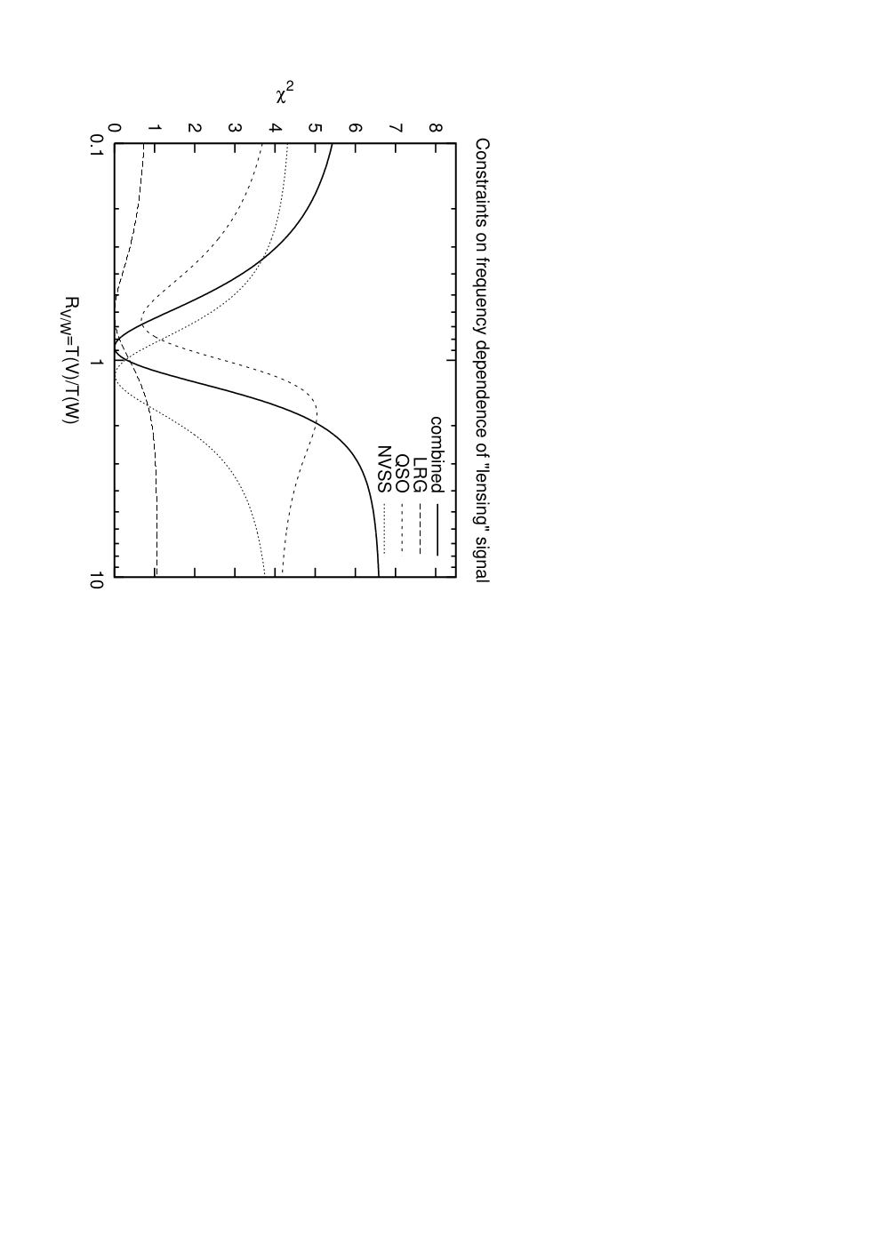
The simplest way to set a constraint on $R_{V/W}$ is as follows. For each LSS sample, we obtained in Section V the amplitudes $A_{VV}$, $A_{VW}$, and $A_{WW}$, which form a 3-component vector ${\bf A}$, and their $3\times 3$ covariance matrix ${\rm Cov}_{\bf A}$ is known from the Monte Carlo simulations. We also know that given $R_{V/W}$ the vector ${\bf A}$ should be parallel to the template vector ${\bf t}(R_{V/W})=(R_{V/W},1,R_{V/W}^{-1})$. Then we construct the $\chi^{2}$:

$$\chi^{2}=\min_{y}[{\bf A}-y{\bf t}(R_{V/W})]^{T}[{\rm Cov}_{\bf A}]^{-1}[{\bf A}-y{\bf t}(R_{V/W})].$$ (35)

The $\chi^{2}$ curves for each sample (LRG, quasar, and NVSS) and the combined case are shown in Figure 6. For the combined case, we find $R_{V/W}=0.87^{+0.74}_{-0.57}$ (2$\sigma$, determined by setting $\chi^{2}-\chi^{2}_{\rm min}=4$).

For each of the LSS samples used in this paper, the frequency dependence of the LSS-convergence correlation is consistent with a blackbody spectrum ($R_{V/W}=1$). In particular for the combined LSS sample, the frequency dependence disfavors the possibility that the signal is due to flat-spectrum radio sources at $2.3\sigma$. With the frequency dependence tests alone, we cannot rule out the possibility that the signal is due to infrared sources or tSZ haloes; our constraints on these contaminants are discussed in Section VII.

Figure 6: Constraints on the frequency dependence of the lensing signal. The horizontal axis is the ratio of thermodynamic temperatures in the V and W bands, which is 1 for the CMB. The vertical axis is the $\chi^{2}$ obtained by fitting the values of the lensing amplitude $A$ in the VV, VW, and WW frequency combinations.

VI.5 Galactic foreground

Galactic foreground emission is an important potential source of systematic error for CMB experiments, including those aiming to study lensing. It arises locally and thus cannot correlate with LSS, but it can correlate with systematic errors in the LRG and quasar maps, such as stellar contamination or errors in the extinction correction. Galactic effects can be treated in basically three ways: (i) one could search for frequency dependence in the maps; or (ii) one could feed an estimate of the Galactic foreground into the lensing estimator and correlate this with the real LSS maps. Of these, (i) is in principle the best if a wide range of frequencies, e.g. the whole WMAP range 23–94 GHz, is available. Unfortunately the lower-frequency bands do not resolve the high multipoles so this approach has limited applicability, and in any case the error bars associated with this approach are large. Therefore we also use (ii), which gives much tighter constraints.

A model for the Galactic foreground must include several known microwave-emitting components. In the V and W bands, thermal emission from dust and free-free radiation from electron-ion collisions are the dominant foregrounds. At the lower WMAP frequencies there is also a soft synchrotron component. In addition, there is an “anomalous” component that dominates at the lower WMAP frequencies and appears to be significant in V band, which may be due to rotational or magnetic dipole emission from dust.

We use a model for the Galactic foreground based on the analysis of [80]; this is the same model as was used in the first-year WMAP lensing analysis [27]. This model is composed of the “Model 8” [81, 82] prediction for thermal dust emission, added to the prediction for free-free radiation based on H$\alpha$ line emission [83] with the conversion factor of [84]. The anomalous microwave emission is included by multiplying the thermal dust template by a factor proportional to $T_{\rm dust}^{2}$, which provides a good phenomenological fit [80]. The soft synchrotron component is negligible in V and W bands, so we do not include it. (In any event, the usual soft synchrotron templates used in CMB work, namely the 408 MHz Haslam maps [85, 86], have a $\sim 50$ arcmin beam that filters out the high multipoles used in the lensing analysis. Use of this map as a foreground indicator for lensing or any other high-$l$ application would give misleading results.)

Since the Galactic emission is not correlated with the CMB, we may estimate the Galactic contamination to the lensing amplitude $\Delta A$ by feeding the Galactic foreground model maps through the lensing pipeline in place of the actual WMAP maps. We computed this for each of the frequency combinations (VV, VW, and WW) and each sample (LRG, quasar, and NVSS); the worst value of the contamination $|\Delta A|$ was $9\times 10^{-4}$. This is negligible compared to our error bars and hence we make no attempt to correct for it.

VII Extragalactic foregrounds

This section considers the major extragalactic foregrounds that can contaminate the lensing signal: point sources; thermal SZ fluctuations; kinetic SZ; and the Rees-Sciama effect. The point sources can be subdivided into “radio” sources, which emit via synchrotron and free-free radiation and are brightest (relative to the CMB) at low frequency, and “infrared” sources, i.e. dusty galaxies. We rely mostly on a combination of frequency and spatial dependence of the foregrounds to separate them from lensing. The brightest radio sources are usually active galactic nuclei (AGN), although star-forming galaxies also emit synchrotron and free-free. Note that it is possible for the same object to be both a radio and an infrared source.

This section is organized as follows. The spatial dependence of foregrounds is discussed in Section VII.1, where we show that the bias in the lensing signal depends on the galaxy-foreground-foreground bispectrum. This bispectrum is decomposed using the halo model and we show how to constrain each term using the galaxy-temperature cross-spectrum $C_{l}^{gT}$ and physical constraints on the point sources such as flux cuts. Most of the rest of the section is based on this framework. We apply the constraints from Section VII.1 to radio point sources in Section VII.2 and infrared sources in Section VII.3. We then investigate the tSZ effect (Section VII.4). Several small effects are considered in the appendices: Appendix C considers the kSZ and ISW/Rees-Sciama effects, and Appendix D considers correlations between different foreground components. The arguments used to constrain the extragalactic foregrounds are summarized in Section VII.5, where we discuss what we believe are the most significant strengths and weaknesses and what could be done to improve them in the future.

VII.1 Point sources: spatial correlation-based tests

Point sources are the most serious foreground for the WMAP lensing analysis. They introduce two major concerns: one is that the artifacts they produce in the lensing map can correlate with large-scale structure, thereby introducing a spurious cross-correlation signal; and they can add power to the lensing map and thus increase the error bars on the cross correlation $C_{l}^{g{\bf v}}$. Neither effect is taken into account in the simulations. However the comparison of the lensing power spectra in Section VI.2 demonstrates that the point sources do not add significantly to the power in the ${\bf v}$ map and hence do not increase the errors $\sigma(C_{l}^{g{\bf v}})$.

We have several methods of constraining the bias in $C_{l}^{Xv}$ due to point sources: (i) tests based on the frequency dependence of the signal; (ii) tests based on spatial correlations; and (iii) tests based on external foreground maps. Of these, (i) was considered in Section VI.4, and (iii) will be discussed using the IRAS maps of dusty sources in Section VII.3.2. This section will focus on the methodology for (ii), the tests using spatial correlations. This methodology is applied to radio sources in Section VII.2 and infrared sources in Section VII.3.

Since our estimates of $C_{l}^{g\kappa}$ are obtained by cross-correlating the LSS map with a “convergence” map that is quadratic in temperature, it follows that any point source contamination must enter via the cross-bispectrum $B_{ll^{\prime}l^{\prime\prime}}^{gTT}$ that contains the LSS tracer and two temperatures. The amount of contamination to the $C_{l}^{g\kappa}$ can be written as

$$\Delta C_{l}^{g\kappa}=R_{l}^{-1}\sum_{l^{\prime}l^{\prime\prime}}{\cal F}_{ll^{\prime}l^{\prime\prime}}B_{ll^{\prime}l^{\prime\prime}}^{gTT}({\rm ps});$$ (36)

see Appendix A for a derivation and Eq. (82) for the definition of the coefficient ${\cal F}_{ll^{\prime}l^{\prime\prime}}$.

We will describe the point source contributions to the cross-bispectrum $B_{ll^{\prime}l^{\prime\prime}}^{gTT}$ in the context of a halo model. Note that since most haloes are unresolved by WMAP, the haloes are described entirely by the number of “galaxies” (LRGS, quasars, NVSS sources) they contain, their microwave flux in each band (in thermodynamic $\mu$K sr), and their 2- and 3-point correlation functions. In most cases we ignore that the haloes are resolved since only the nearest haloes are resolved and in any case we have directly tested that an NFW profile leads to a lower contamination to the lensing signal than a delta function with the same integrated flux. Since very little information is available on the halo occupation distributions (HODs) for quasars, NVSS sources, and microwave sources, our analysis will be based to the maximum extent possible on general properties of the halo model; in particular we will avoid parameterized HODs entirely.

Within the context of the halo model, the point source contributions to the cross-bispectrum $B_{ll^{\prime}l^{\prime\prime}}^{gTT}$ can have four contributions:

• The “1-halo” term, which arises when the two factors of temperature come from point sources in the same halo as the galaxy.

• The “2a-halo” term, in which the two factors of temperature come from point sources in the same halo, but the galaxy is in a different halo.

• The “2b-halo” term, in which there is one point source in the same halo as the galaxy and the other point source lives in a different halo.

• The “3-halo” term, in which the galaxy and both point sources live in three distinct halos.

Note that there can be no galaxy-point source-primary CMB cross-bispectrum since the primary CMB resides at $z\sim 1100$ whereas the galaxies and point sources are at much lower $z$.

The formulas for $B_{ll^{\prime}l^{\prime\prime}}^{gTT}$ are simply stated here so that we can concentrate on the physical assumptions required by our argument; derivations for the 1- and 2-halo terms can be found in Appendix B, while the 3-halo term is derived by the usual Limber argument (see e.g. Ref. [87]). The number of galaxies $N$ and microwave flux $F$ of a halo are of course dependent not only on the intrinsic properties of the halo but also on the redshift, since flux declines as the luminosity distance squared (times the $k$-correction) and the selection criteria for our samples are redshift-dependent. For brevity we will not write this dependence explicitly. The 1- and 2-halo terms make use of the maximum unmasked point source flux $F_{\rm max}$ and the maximum number of galaxies per halo $N_{\rm max}$. We use the notation $\rho(F)\,dF$ is the comoving 3-dimensional number density of haloes emitting microwave flux between $F$ and $F+dF$ and $\rho(N)$ to denote the comoving 3-dimensional number density of haloes with $N$ galaxies. The 2-dimensional (projected) number densities will be denoted $n_{2D}(F)$ and $n_{2D}(N)$. We will also use the notation

$$f(\chi)\equiv\bar{n}_{g}^{-1}r^{2}\sum_{N}N\rho(N)b(N)=\frac{dz}{d\chi}f(z)$$ (37)

for the bias-weighted comoving distance distribution of the galaxies.

We will consider the 1- and 2a-halo terms together, since they are closely related, and then the 2b- and 3-halo terms separately. We will use two separate ways of estimating the 1- and 2a-halo terms. Method I uses the cross-power spectra $C_{l}^{gT}$ obtained in Paper I, and crudely speaking the basic idea is that for 1- and 2a-halo terms, the conversion factor from power spectrum to bispectrum cannot be greater than the maximum flux $F_{\rm max}$. Method II looks at the bispectrum of the galaxies and two frequency-differenced maps to constrain the $F^{2}$-weighted correlation function of the galaxies and the point sources. Generally for types of sources that are very faint, i.e. where $F_{\rm max}$ is below the WMAP noise level per beam, Method I gives the tighter constraint, whereas for radio sources (which can be extremely bright) Method II is superior.

VII.1.1 1- and 2a-halo terms: General considerations

The 1-halo contribution to the cross-bispectrum is simply the Poisson bispectrum,

$$B_{ll^{\prime}l^{\prime\prime}}^{gTT}({\rm 1h})=\eta_{ll^{\prime}l^{\prime\prime}}\int dF\sum_{N}\frac{NF^{2}}{\bar{n}_{g}}n_{2D}(N,F),$$ (38)

where $F$ is the halo flux, $N$ is the number of galaxies in the halo, $\bar{n}_{g}$ is the mean number of galaxies per steradian, and $n_{2D}(N,F)\,dF$ is the number of haloes per steradian containing $N$ galaxies and with flux between $F$ and $F+dF$. The coefficient $\eta_{ll^{\prime}l^{\prime\prime}}$ is given by

$$\eta_{ll^{\prime}l^{\prime\prime}}=\sqrt{\frac{(2l+1)(2l^{\prime}+1)(2l^{\prime\prime}+1)}{4\pi}}\left(\begin{array}[]{ccc}l&l^{\prime}&l^{\prime\prime}\\ 0&0&0\end{array}\right),$$ (39)

and simply encodes the products of spherical harmonics. Usually Eq. (38) would be written in terms of 3-dimensional densities and then integrated over redshift (or comoving distance $\chi$) using the Limber approximation. This is useful for theoretical predictions since theory usually gives 3-dimensional densities and biases of haloes as a function of mass and redshift, and does not directly give results in projection. However in our case both the desired constraint (on $B_{ll^{\prime}l^{\prime\prime}}^{gTT}$) and the given information ($C_{l}^{XT}$ measured from Paper I) are already projected onto the sky, so we can derive our constraints entirely with Eq. (38) without considering the 3-dimensional distribution of the point sources.

The analogous equation to Eq. (38) for the 2a-halo term is

$$B_{ll^{\prime}l^{\prime\prime}}^{gTT}({\rm 2ah}) = \eta_{ll^{\prime}l^{\prime\prime}}\int dF\sum_{N}\frac{NFF^{\prime}}{\bar{n}_{g}}$$ (40)

$$\times n_{2D}(N)n_{2D}(F)C_{l}(N;F),$$

where $n_{2D}(N)$ is the 2-dimensional density (objects per steradian) of haloes with $N$ galaxies; $n_{2D}(F)\,dF$ is the 2-dimensional density of haloes emitting flux between $F$ and $F+dF$; and $C_{l}(N;F)$ is the cross-power spectrum between haloes containing $N$ galaxies and haloes with flux $F$. This cross-power does not include shot noise. Once again for the sake of ab initio theoretical predictions it would be most useful to write this as a Limber integral, containing 3-dimensional instead of 2-dimensional densities and involving the 3-dimensional cross-spectrum between different types of haloes; but for our purposes we can work entirely in the 2-dimensional space.

This implies a combined 1+2a-halo contribution to the cross-bispectrum,

$$B_{ll^{\prime}l^{\prime\prime}}^{gTT}(1+{\rm 2ah}) = \eta_{ll^{\prime}l^{\prime\prime}}\int dF\sum_{N}\frac{NF^{2}}{\bar{n}_{g}}[n_{2D}(N,F)$$ (41)

$$+n_{2D}(N)n_{2D}(F)C_{l}(N;F)].$$

The corresponding bias in the cross-power is obtained from Eq. (36):

$$\Delta C_{l}^{g\kappa}(1+{\rm 2ah}) = R_{l}^{-1}\left(\sum_{l^{\prime}l^{\prime\prime}}{\cal F}_{ll^{\prime}l^{\prime\prime}}\eta_{ll^{\prime}l^{\prime\prime}}\right)$$ (42)

$$\times\int dF\sum_{N}\frac{NF^{2}}{\bar{n}_{g}}[n_{2D}(N,F)$$

$$+n_{2D}(N)n_{2D}(F)C_{l}(N;F)].$$

Note that $l^{\prime}$ and $l^{\prime\prime}$ enter only in the summation in parentheses, a fact that will prove to be extremely valuable. This “compartmentalization” is a direct result of the pointlike nature of the sources under consideration. It is convenient to define $r_{ps}(l)$ to be the combination in parentheses (this is consistent with the definition in Ref. [27]), so that

$$\Delta C_{l}^{g\kappa}(1+{\rm 2ah}) = \frac{r_{ps}(l)}{R_{l}}\int dF\sum_{N}\frac{NF^{2}}{\bar{n}_{g}}[n_{2D}(N,F)$$ (43)

$$+n_{2D}(N)n_{2D}(F)C_{l}(N;F)].$$

The point source responsivity $r_{ps}(l)/R_{l}$ is negative for $l\leq 269$. This is a measure of the spurious lensing signal that is produced by a point source as a function of scale. Note in particular that if the galaxies and point sources are positively correlated, i.e.

$$\sum_{N}N[n_{2D}(N,F)+n_{2D}(N)n_{2D}(F)C_{l}(N;F)]\geq 0,$$ (44)

then the bias $\Delta C_{l}^{g\kappa}$(1+2ah) must have the same sign as $r_{ps}(l)/R_{l}$. Note that for $l\leq 269$ we have $r_{ps}(l)/R_{l}$; this is simply a statement that the long-wavelength ($l\leq 269$) modes of the reconstructed lensing map have a negative-convergence artifact around each point source. Since our fits to the lensing amplitude $A$ use only the $l\leq 269$ multipoles, it follows that it is not possible for the observed lensing signal to be due to the 1- or 2a-halo point source terms (i.e. artifacts in the ${\bf v}$ map that arise from individual sources rather than interference between sources clustered with each other). It is possible for the amplitude $A$ to be biased downward (at some level it must be) and this must be considered in any cosmological analysis.

VII.1.2 1- and 2a-halo terms: Method I

Our objective here is to set a constraint on the possible contamination, Eq. (43). To do this, we consider the cross-spectrum of the galaxies and the temperature, $C_{l}^{gT}$, coming from the point sources. This is a relatively simple calculation that has only 1- and 2-halo contributions; the answer is

$$C_{l}^{gT}({\rm ps}) = \int dF\sum_{N}\frac{NF}{\bar{n}_{g}}[n_{2D}(N,F)$$ (45)

$$+n_{2D}(N)n_{2D}(F)C_{l}(N;F)].$$

We now note that the integral over $dF$ in Eq. (43) is identical to $C_{l}^{gT}({\rm ps})$ except for an additional factor of $F$. If we make the assumption that the fluxes are less than some $F_{\rm max}$, and also assume that the integrand is nonnegative (Eq. 44), it follows that the integral over $dF$ in Eq. (43) is bounded between 0 and $F_{\rm max}C_{l}^{gT}({\rm ps})$. Then we can conclude that (i) the contamination $\Delta C_{l}^{g\kappa}(1+{\rm 2ah})$ has the same sign as $r_{ps}(l)$, and (ii) the contamination is bounded by

$$|\Delta C_{l}^{g\kappa}(1+{\rm 2ah})|\leq\frac{F_{\rm max}}{R_{l}}\left|r_{ps}(l)\right|C_{l}^{gT}({\rm ps}).$$ (46)

This simple inequality, which allows us to estimate the point source contamination, relies only on the existence of a bound on the point source flux, and the requirement of Eq. (44), i.e. that galaxies and point sources are positively correlated (where the correlation includes the Poisson term). Note that aside from the positivity of the correlation no assumption is made about the halo mass function, bias, environment dependence or lack thereof, etc., so we believe this represents a very robust bound.

VII.1.3 1- and 2a-halo terms: Method II

We now consider another way to constrain the 1- and 2a-halo terms. This time, instead of using a maximum flux $F_{\rm max}$, we attempt to directly measure the integral in Eq. (43) using a quantity quadratic in the CMB temperature and linear in the galaxy density. We do this using frequency-differenced maps, which renders our point source analysis completely insensitive to biases produced by lensing of the CMB, and to noise produced by the primary CMB anisotropy. This method is useful only for the radio point sources since for these Method I is not very constraining (due to large $F_{\rm max}$).

The basic idea is that we produce two frequency-difference maps $D^{(1)}$ and $D^{(2)}$. In the simplest version of the method, the map $D^{(1)}$ is the difference of the WMAP temperature maps $T(Ka)-T(V)$, both smoothed to the resolution of the Ka-band map. The map $D^{(2)}$ is similarly constructed from $T(Q)-T(W)$. We will denote the effective (post-smoothing) beam transfer functions $B^{(1)}_{l}$ and $B^{(2)}_{l}$. We then multiply the two maps to produce $D(\hat{\bf n})=D^{(1)}(\hat{\bf n})D^{(2)}(\hat{\bf n})$. The idea is that each point source produces a feature in $D(\hat{\bf n})$ whose intensity is proportional to $F^{2}$ and various factors that involve the frequency dependence. Specifically, if the input map contains a single point source, then the output map intensity can be shown to equal

$$D_{lm}=K^{(1)}K^{(2)}F_{V,i}^{2}\tau_{l}Y_{lm}^{\ast}(\hat{\bf n}_{i}),$$ (47)

where $\hat{\bf n}_{i}$ is the position of the point source, $F_{V,i}$ is its V-band flux (in units of $\mu$K sr), $\tau_{l}$ is the transfer function

$$\tau_{l}=\sum_{l^{\prime}l^{\prime\prime}}\frac{(2l^{\prime}+1)(2l^{\prime\prime}+1)}{4\pi}B^{(1)}_{l^{\prime}}B^{(2)}_{l^{\prime\prime}}\left(\begin{array}[]{ccc}l&l^{\prime}&l^{\prime\prime}\\ 0&0&0\end{array}\right)^{2},$$ (48)

and the spectral-dependent terms are $K^{(1)}=(F_{Ka,i}-F_{V,i})/F_{V,i}$ and similarly for $K^{(2)}$. (This formula follows immediately from the multiplication in real space of the two beams.) If the map contains multiple point sources then in addition to terms of the form Eq. (47) there are interference terms involving combinations of two point sources (with different sources contributing to $D^{(1)}$ and $D^{(2)}$). We may then do a cross-correlation with the galaxies, $C_{l}^{gD}$. The 1+2a halo contributions (i.e. leaving out the interference contribution to $D$) to this are

$$C_{l}^{gD}(1+{\rm 2ah})=K^{(1)}K^{(2)}\tau_{l}\int dF\,n_{2D}(F)F^{2}C_{l}(g,F),$$ (49)

where $C_{l}(g,F)$ is the angular cross-spectrum between galaxies and haloes of flux $F$. This can be expanded as

$$C_{l}^{gD}(1+{\rm 2ah}) = K^{(1)}K^{(2)}\tau_{l}\int dF\sum_{N}\frac{NF^{2}}{\bar{n}_{g}}[n_{2D}(N,F)$$ (50)

$$+n_{2D}(N)n_{2D}(F)C_{l}(N;F)],$$

so that

$$\Delta C_{l}^{g\kappa}(1+{\rm 2ah})=\frac{r_{ps}(l)}{R_{l}}\frac{C_{l}^{gD}(1+{\rm 2ah})}{K^{(1)}K^{(2)}\tau_{l}}.$$ (51)

We use this equation to estimate the 1+2a halo point source contamination of $C_{l}^{g\kappa}$.

In this method it is important to remove the Galactic foreground, particularly since one is working with the low-frequency bands where the Galaxy is brightest. There are two ways to do this. One is to subtract the Galactic foreground model (Section VI.5). Alternatively, instead of directly multiplying the maps $D^{(i)}$, one can high-pass filter them, which should remove more of the slowly varying Galactic signal. The latter method also has the advantage that the temperature offsets in the different bands is not needed (WMAP does not measure these directly and used a simple model of the Galaxy to set these offsets). A simple, local high-pass filter is to subtract the map smoothed by a Gaussian of width $\sigma_{1}=45\,$arcmin; this is equivalent to modifying the effective beam in accordance with

$$B^{(i)}\rightarrow B^{(i)}[1-e^{-l(l+1)\sigma_{1}^{2}/2}].$$ (52)

Thus $\tau_{l}$ is different for the two methods.

VII.1.4 2b-halo term

The analogous equation to Eq. (38) for the 2b-halo term is

$$\!\!\!\!B_{ll^{\prime}l^{\prime\prime}}^{gTT}({\rm 2bh}) = \eta_{ll^{\prime}l^{\prime\prime}}\int dF\int dF^{\prime}\sum_{N}\frac{NFF^{\prime}}{\bar{n}_{g}}$$ (53)

$$\times n_{2D}(N,F)n_{2D}(F^{\prime})$$

$$\times[C_{l^{\prime}}(N,F;F^{\prime})+C_{l^{\prime\prime}}(N,F;F^{\prime})],$$

where $n_{2D}(N)$ is the 2-dimensional density (objects per steradian) of haloes with $N$ galaxies; $n_{2D}(F)\,dF$ is the 2-dimensional density of haloes emitting flux between $F$ and $F+dF$; and $C_{l}(N,F;F^{\prime})$ is the cross-power spectrum between haloes containing $N$ galaxies with flux $F$ and haloes with flux $F^{\prime}$. The spurious contribution to the galaxy-convergence correlation is obtained from Eq. (36):

$$\Delta C_{l}^{g\kappa}({\rm 2bh}) = 2R_{l}^{-1}\sum_{l^{\prime}l^{\prime\prime}}{\cal F}_{ll^{\prime}l^{\prime\prime}}\eta_{ll^{\prime}l^{\prime\prime}}$$ (54)

$$\times\int dF\int dF^{\prime}\sum_{N}\frac{NFF^{\prime}}{\bar{n}_{g}}$$

$$\times n_{2D}(N,F)n_{2D}(F^{\prime})C_{l^{\prime}}(N,F;F^{\prime}).\;\;\;\;$$

Here we have removed the $C_{l^{\prime\prime}}(N,F;F^{\prime})$ term and doubled the result because of the symmetry of ${\cal F}$ and $\eta$ under interchange of $l^{\prime}$ and $l^{\prime\prime}$.

We would like to place a bound on $\Delta C_{l}^{g\kappa}({\rm 2bh})$ using the galaxy-temperature cross power spectrum, just as was done for the 1- and 2a-halo terms in Method I. There are two simple ways of doing this: one based on the maximum flux $F_{\rm max}$, and the other based on the maximum number of galaxies per halo $N_{\rm max}$. The former is model-independent and is preferred, except for the radio sources for which it does not give an interesting constraint due to large $F_{\rm max}$.

The $F_{\rm max}$ method works by using the triangle inequality in Eq. (54), and then noting that $F\leq F_{\rm max}$:

$$|\Delta C_{l}^{g\kappa}({\rm 2bh})| \leq 2R_{l}^{-1}\sum_{l^{\prime}}\left|\sum_{l^{\prime\prime}}{\cal F}_{ll^{\prime}l^{\prime\prime}}\eta_{ll^{\prime}l^{\prime\prime}}\right|$$ (55)

$$\times\int dF^{\prime}\sum_{N}\frac{NF_{\rm max}F^{\prime}}{\bar{n}_{g}}$$

$$\times n_{2D}(N)n_{2D}(F^{\prime})C_{l^{\prime}}(N;F^{\prime}).$$

The last two lines in this equation are – aside from the factor of $F_{\rm max}$ – equal to the 2-halo galaxy-temperature spectrum. This must be less than or equal to the actual galaxy-temperature spectrum since the 1-halo term must be nonnegative, so we may write

$$|\Delta C_{l}^{g\kappa}({\rm 2bh})| \leq 2R_{l}^{-1}\sum_{l^{\prime}}\left|\sum_{l^{\prime\prime}}{\cal F}_{ll^{\prime}l^{\prime\prime}}\eta_{ll^{\prime}l^{\prime\prime}}\right|$$ (56)

$$\times F_{\rm max}C_{l^{\prime}}^{gT}({\rm ps}).$$

The last cross-spectrum was directly measured out to $l^{\prime}=600$. It is extrapolated to higher $l^{\prime}$ assuming $C_{l^{\prime}}^{gT}=$constant, which is conservative since the 2-halo $C_{l^{\prime}}$ decreases at high multipole [due to the declining $P(k)$ over the relevant range of scales].

The model-dependent $N_{\rm max}$ method works as follows. Written in terms of angular correlations, the 2-halo contribution to the point source power spectrum is

$$C_{l}^{TT}({\rm ps,2h}) = \int dF\int dF^{\prime}\,FF^{\prime}n_{2D}(F)$$ (57)

$$\times n_{2D}(F^{\prime})C_{l^{\prime}}(F;F^{\prime}).$$

We then have

$$|\Delta C_{l}^{g\kappa}({\rm 2bh})| \leq 2R_{l}^{-1}\sum_{l^{\prime}}\left|\sum_{l^{\prime\prime}}{\cal F}_{ll^{\prime}l^{\prime\prime}}\eta_{ll^{\prime}l^{\prime\prime}}\right|$$ (58)

$$\times\frac{N_{\rm max}}{\bar{n}_{g}}C_{l^{\prime}}^{TT}({\rm ps,2h}),$$

where $N_{\rm max}$ is the maximum number of galaxies found in a halo and we have assumed the positivity condition

$$\sum_{N}NC_{l}(N,F;F^{\prime})\geq 0.$$ (59)

On the other hand, written in terms of a Limber integral, $C_{l}^{TT}$(ps,2h) is

$$C_{l}^{TT}({\rm ps,2h})=\int\frac{d\chi}{r^{2}}[b_{T}\bar{T}^{\prime}(\chi)]^{2}P_{\rm lin}(k)$$ (60)

where $P_{\rm lin}(k)$ is the linear power spectrum at $k=(l+1/2)/r$,

$$\bar{T}^{\prime}(\chi)\equiv r^{2}\int dF\,F\rho(F)$$ (61)

is the mean contribution to the brightness temperature per unit comoving distance, and

$$b_{T}\equiv\frac{\int dF\,F\rho(F)b(F)}{\int dF\,F\rho(F)}$$ (62)

is the effective (flux-weighted) bias of the microwave emitters. We note that $\bar{T}^{\prime}(\chi)$ does not diverge at small distances even though the fluxes from certain haloes can become large because of the $r^{2}$ factor; this can be seen explicitly from the relation

$$\bar{T}^{\prime}(\chi,\nu)=\frac{c^{2}}{2k_{\rm B}\nu^{2}}(1+z)\bar{j}^{\rm com}_{\nu(1+z)},$$ (63)

where $\nu$ is the observed frequency, $\bar{j}^{\rm com}_{\nu}$ is the comoving emissivity (in e.g. erg cm${}^{-3}\,$s${}^{-1}\,$Hz${}^{-1}\,$sr^-1, where the cm are comoving and all other units are physical), and $k_{\rm B}$ is Boltzmann’s constant.

This equation is not quite in a usable form, since the intensity and redshift distribution ($\bar{T}^{\prime}$) and bias ($b_{T}$) of the non-primordial background are still unknown. Therefore we have tried a different approach. Using the Limber approximation, and assuming linear biasing, the second (2-halo) term of Eq. (45) can be rewritten as

$$\!\!\!\!C_{l}^{gT} \geq C_{l}^{gT}({\rm 2h})$$ (64)

$$= \int d\chi\,r^{2}\int dF\sum_{N}\frac{NF}{\bar{n}_{g}}\rho(F)\rho(N)$$

$$\times b(F)b(N)P_{\rm lin}(k),$$

$$= \int\frac{d\chi}{r^{2}}f(\chi)b_{T}\bar{T}^{\prime}(\chi)P_{\rm lin}(k).$$

Physically we expect the bias $b_{T}$ to vary slowly with redshift. The same is also true of $\bar{j}_{\nu}$ and hence $\bar{T}^{\prime}(\chi)$ (see Eq. 63). If over the range of redshifts of interest it is a power law, $b_{T}\bar{T}^{\prime}(\chi)\propto(1+z)^{\zeta}$, then

$$b_{T}\bar{T}^{\prime}(\chi)|_{z=0}\leq\frac{C_{l_{0}}^{XT}}{\int d\chi\,r^{-2}f(\chi)(1+z)^{\zeta}P_{\rm lin}(k_{0})},$$ (65)

where equality would hold if the right-hand side included only the two-halo term, $l_{0}$ is any arbitrary multipole, and $k_{0}=(l_{0}+1/2)/r$. In practice to increase signal-to-noise ratio, we average the right-hand side over all the multipole bins between 25 and $l_{\rm max}$ (the multipole corresponding to $k=0.1h\,$Mpc^-1 at the 20th percentile in distance). We construct bounds on the 2b-halo point source contamination by considering a range of exponents $\zeta$. Of course, all of these integrals to the redshift range where there are galaxies; we use $z_{\rm max}=0.8$ for the LRGs, 2.7 for the quasars, and 3 for NVSS.

For the quasars and the NVSS galaxies the constraint on the maximum number of galaxies per halo will be redshift-dependent. In this case, it is straightforward to show that Eq. (58) undergoes the replacement

$$N_{\rm max}C_{l^{\prime}}^{TT}({\rm ps,2h})\rightarrow\int\frac{d\chi}{r^{2}}N_{\rm max}(\chi)[b_{T}\bar{T}^{\prime}(\chi)]^{2}P_{\rm lin}(k),$$ (66)

i.e. $N_{\rm max}$ is pulled inside the integral over comoving distance (or redshift).

VII.1.5 3-halo term

The 3-halo contribution to the point source bispectrum is different from the 1- and 2-halo terms in that we have found no simple model-independent argument to constrain it using the galaxy-temperature correlation. Instead we will have to use a more model-dependent method. The Limber equation allows us to express the galaxy-temperature-temperature angular bispectrum in terms of the 3-dimensional bispectrum,

$$B_{ll^{\prime}l^{\prime\prime}}^{gTT}({\rm 3h}) = \eta_{ll^{\prime}l^{\prime\prime}}\int d\chi\,r^{2}\int dF\int dF^{\prime}\sum_{N}\rho(N)\rho(F)$$ (67)

$$\times\rho(F^{\prime})\frac{NFF^{\prime}}{\bar{n}_{X}}B(k,k^{\prime},k^{\prime\prime}|N;F;F^{\prime}),$$

where $\chi$ is the radial comoving distance; $r$ is the comoving angular diameter distance (equal to $\chi$ for a flat universe); $\rho(N)$ is the comoving number density of haloes containing $N$ galaxies; $\rho(F)dF$ is the comoving number density of haloes with microwave flux between $F$ and $F+dF$; the wavenumbers are $k=(l+1/2)/r$, etc.; and $B(k,k^{\prime},k^{\prime\prime}|N;F;F^{\prime})$ is the 3-dimensional cross-bispectrum of the haloes with $N$ galaxies, the haloes with flux $F$, and the haloes with flux $F^{\prime}$. The problem is that the key quantities $\rho(F)$ and $B(k,k^{\prime},k^{\prime\prime}|N;F;F^{\prime})$ are not known.

To circumvent this problem, we will consider the linear bias prediction for the 3-halo term. That is, we set

$$B(k,k^{\prime},k^{\prime\prime}|N;F;F^{\prime})=b(N)b(F)b(F^{\prime})B_{\rm 2P}(k,k^{\prime},k^{\prime\prime}),$$ (68)

where $b$ represents the bias of the haloes and $B_{\rm 2P}(k,k^{\prime},k^{\prime\prime})$ is the second-order perturbation theory bispectrum. This allows us to factor Eq. (67), yielding

$$B_{ll^{\prime}l^{\prime\prime}}^{gTT}=\eta_{ll^{\prime}l^{\prime\prime}}\int\frac{d\chi}{r^{4}}f(\chi)[b_{T}\bar{T}^{\prime}(\chi)]^{2}B_{\rm 2P}(k,k^{\prime},k^{\prime\prime}).$$ (69)

Using Eq. (36), we may then write

$$|\Delta C_{l}^{g\kappa}({\rm 3h})| \leq R_{l}^{-1}\sum_{l^{\prime}l^{\prime\prime}}\Bigl|{\cal F}_{ll^{\prime}l^{\prime\prime}}\eta_{ll^{\prime}l^{\prime\prime}}\int\frac{d\chi}{r^{4}}$$ (70)

$$\times f(\chi)[b_{T}\bar{T}^{\prime}(\chi)]^{2}B_{\rm 2P}(k,k^{\prime},k^{\prime\prime})\Bigr|.$$

The factor $b_{T}\bar{T}^{\prime}(\chi)$ comes from the bound, Eq. (65), just as for the 2b-halo term ($N_{\rm max}$ method). Like the 2b-halo term, it is model-dependent. Fortunately, the bound is also very small so deviations of halo clustering from the simple perturbation theory predictions or more complicated redshift evolution of $b_{T}\bar{T}^{\prime}(\chi)$ will have little effect.

VII.2 Estimates of contamination: radio sources

We now construct radio point source contamination estimates using the methodology of the previous section. For the 2b- and 3-halo terms we need to know the contribution to the cross-spectra $C_{l}^{gT}$ from radio sources in order to get $b_{T}\bar{T}^{\prime}$. We will use only Method II for the 1+2a-halo terms because for the bright radio sources Method I does not give an interesting constraint.

The $C_{l}^{gT}$ cross-powers for the LRGs, the SDSS quasars, and the NVSS sources were obtained in Paper I in the range up to $l=600$. Unfortunately they are noisy, with the noise dominated by primary CMB fluctuations, and on large angular scales the ISW effect dominates the cross-power. For this reason, we have used the differences $C_{l}^{gT}(Q)-C_{l}^{gT}(V)$ and $C_{l}^{gT}(V)-C_{l}^{gT}(W)$ as the major sources of information on point sources. We construct our estimates for the V-band lensing estimator, which will be the most contaminated by radio sources. For flat spectrum sources and the relative weighting of bands in Eq. (24), the ratio of contamination is

$$\frac{\Delta C_{l}^{g\kappa}(TT)}{\Delta C_{l}^{g\kappa}(VV)}=0.56.$$ (71)

We take as our estimate of the radio point source cross-spectrum

$$\hat{C}_{l}^{gT}(V;{\rm rps}) \equiv a_{1}[C_{l}^{gT}(Q)-C_{l}^{gT}(V)]$$ (72)

$$+a_{2}[C_{l}^{gT}(V)-C_{l}^{gT}(W)],$$

with $a_{1}=1.128$ and $a_{2}=-0.466$. The ratio $a_{2}/a_{1}=-0.413$ is chosen to cancel any tSZ contribution, and the normalization was chosen to be correct for flat-spectrum radio sources with $F_{\nu}=$constant. If there are also steep-spectrum sources this is an overestimate of their effect: for $F_{\nu}\propto\nu^{-0.8}$ we have $\hat{C}_{l}^{gT}(V;{\rm rps})=1.66C_{l}^{gT}(V;{\rm rps})$. Equation (72) has some sensitivity to infrared sources: for $F_{\nu}\propto\nu^{3.5}$ we have $\hat{C}_{l}^{gT}(V;{\rm rps})=0.008C_{l}^{gT}(V;{\rm dust})$, and the coefficient 0.008 rises to 0.146 if $F_{\nu}\propto\nu^{4}$. Since this coefficient is positive we will overestimate the contribution of radio sources if the infrared sources are also significant. This cross-spectrum is obtained by constructing a WMAP map of the frequency combination 1.128Q-1.594V+0.466W and cross-correlating it with each galaxy map. Also in order to speed up the calculation we did not implement any weighting in the $C_{l}^{gT}$ estimation, i.e. instead of full ${\bf C}^{-1}$ weighting we only project out the monopole and dipole from each map (and in the case of NVSS, the declination rings and Haslam map). We have computed error bars for each case by cross-correlating 20 simulated LSS maps with the actual WMAP difference map (on large angular scales in WMAP the difference maps contain $1/f$ noise and Galactic foregrounds, and hence are more difficult to reliably simulate than the LSS maps). The simulated LSS maps are Gaussian and have the correct autopower spectra as determined from Paper I. The Gaussianity of the LSS does not matter for getting the variance of $C_{l}^{gT}(V;{\rm rps})$, since the $C_{l}^{gT}(V;{\rm rps})$ estimator is a linear function of the data.

The 2b- and 3-halo terms can be constrained if we know the maximum number of galaxies per halo $N_{\rm max}$ (needed for the 2b-halo term only) and the redshift evolution exponent $\zeta=d\ln[b_{T}\bar{T}^{\prime}(\chi)]/d\ln(1+z)$. We estimate $N_{\rm max}$ for NVSS by examining each object and finding the number of neighbors (including the object itself) within 6 arcminutes ($\sim 1h^{-1}\,$Mpc at $z=0.2$). For NVSS there are no objects with $>12$ neighbors, 1 with 12 neighbors, and 2 with 11 neighbors, so we set $N_{\rm max}=12$. This may be a large overestimate: in particular Poisson statistics predicts 0.1 objects with 12 neighbors and 0.9 with 11 neighbors, so it is not clear that these groupings should be taken seriously. Nevertheless for our purposes all we need is an upper limit, so we use 12. For the quasars the maximum number of neighbors is 10, so we set $N_{\rm max}=10$. Again this should not be taken especially seriously (for Poisson statistics there should be on average 1.2 objects with 10 neighbors). For the LRGs a similar argument gives $N_{\rm max}=36$. For quasars and NVSS the redshift distribution extends to higher $z$ where we can improve the constraint on $N_{\rm max}$. For example at $z=0.8$ a $1h^{-1}\,$Mpc radius corresponds to 2 arcminutes; thus for $z\geq 0.8$ we have replaced the above $N_{\rm max}$ values with the maximum number of neighbors within 2 arcmin. This is 5 for the quasars and 5 for NVSS. For NVSS we have also set $N_{\rm max}=3$ for $z\geq 3$, which is what we find with a 45 arcsec radius ($1h^{-1}\,$Mpc at $z=3$).

We do not know the redshift dependence of $b_{T}\bar{T}^{\prime}$ so we have to consider a range of possibilities and determine which leads to the most serious contamination. This is done for power laws $b_{T}\bar{T}^{\prime}\propto(1+z)^{\zeta}$ in the last part of Table 3 (note that flat spectrum sources with constant comoving density would have $\zeta=2$). Note that the 2b- and 3-halo terms are shown to be negligible. For $\zeta=0$ we find upper limits to $b_{T}\bar{T}^{\prime}(\chi)$ to be $(0\pm 5)h\,$nK Mpc^-1 for the LRGs, $(-6\pm 11)h\,$nK Mpc^-1 for the quasars, and $(+1\pm 2)h\,$nK Mpc^-1 for NVSS; these are upper limits because they assume the entire correlation comes from the 2-halo term. The combined 95% confidence upper limit is $4h\,$nK Mpc^-1. This is a one-tailed upper limit ($+1.64\sigma$) since physially $b_{T}\bar{T}^{\prime}$ should be positive.

We now apply Method II (Section VII.1.3) to the 1+2a halo term. For the method based on $Ka-V$ and $Q-W$ differences, and for flat-spectrum sources the flux ratios $(F_{Ka}-F_{V})/F_{V}$ and $(F_{Q}-F_{W})/F_{V}$ are 2.20 and 1.63, respectively, so that $K^{(1)}K^{(2)}=3.57$. The transfer function $T_{l}$ varies from $5.0\times 10^{3}$ to $3.0\times 10^{3}$ as $l$ varies from 0 to 400. The implied bias $\Delta A$ is given in Table 3. We have shown this for both cases where the Galactic foreground model is subtracted (“Gs”) and where it is removed by high-pass filtering (“hpf”). We have also shown this for different combinations of frequency bands. In cases where the same band appears twice, e.g. (Ka$-$V)(Q$-$V), we have computed only cross-correlations involving different DAs and averaged the results, e.g. “(Ka$-$V)(Q$-$V)” is actually the average of (Ka$-$V1)(Q$-$V2) and (Ka$-$V2)(Q$-$V1). Just as for Method I we compute error bars using simulated LSS maps since it is harder to simulate the product-difference maps.

Table 3: Estimates of the radio point source contamination $|\Delta A|$ to the galaxy-convergence correlation amplitude $A$. The estimates are referenced to the VV lensing maps; for flat-spectrum sources the contamination to TT is reduced by a factor of 0.56. We consider separately the contribution from the 1+2a, 2b, and 3-halo terms. The first part of the table consists of upper limits; the subscript “max” is used to emphasize that these are estimates of an upper limit. In particular $|\Delta A|_{\rm max}$ can be used to assess the magnitude of systematic errors but should not be used to “correct” the data! The bottom part of the table contains estimates of the contamination – these are “central” values and their errors (where shown) are $1\sigma$ statistical errors, not including any uncertainty in the frequency dependence of the foreground. The notations “Gs” and “hpf” are used to indicate that the Galactic foreground is subtracted (Gs) from the difference maps $D^{(1,2)}$, or that it is removed by high-pass filtering (hpf); see Section VII.1.3.

Term		Method/assumption		$|\Delta A|_{\rm max}$(LRG)		$|\Delta A_{\rm max}|$(QSO)		$|\Delta A|_{\rm max}$(NVSS)
2b halo		$\zeta=+4$, fiducial cosmology		$8.8\times 10^{-4}$		$2.8\times 10^{-2}$		$4.0\times 10^{-2}$
2b halo		$\zeta=0$, fiducial cosmology		$5.6\times 10^{-3}$		$6.2\times 10^{-3}$		$7.0\times 10^{-3}$
2b halo		$\zeta=-4$, fiducial cosmology		$1.8\times 10^{-2}$		$1.6\times 10^{-2}$		$1.9\times 10^{-2}$
3 halo		$\zeta=0$, fiducial cosmology		$1.2\times 10^{-3}$		$1.4\times 10^{-4}$		$4.3\times 10^{-4}$
3 halo		$\zeta=+4$, fiducial cosmology		$1.7\times 10^{-4}$		$6.5\times 10^{-4}$		$4.2\times 10^{-4}$
3 halo		$\zeta=-4$, fiducial cosmology		$1.7\times 10^{-3}$		$1.4\times 10^{-4}$		$1.1\times 10^{-3}$
Term		Method/assumption		$\Delta A$(LRG)		$\Delta A$(QSO)		$\Delta A$(NVSS)
1+2a halo		Method II, (Ka$-$V)(Q$-$W), hpf		$+0.060\pm 0.045$		$+0.039\pm 0.040$		$+0.041\pm 0.037$
1+2a halo		Method II, (Ka$-$V)(Q$-$W), Gs		$+0.001\pm 0.076$		$-0.007\pm 0.062$		$-0.023\pm 0.034$
1+2a halo		Method II, (Ka$-$V)(Q$-$V), hpf		$+0.005$		$-0.013$		$+0.046$
1+2a halo		Method II, (K$-$Q)(Ka$-$V), hpf		$+0.032$		$+0.013$		$+0.021$
1+2a halo		Method II, (Ka$-$V)(Q$-$V), Gs		$-0.090$		$-0.009$		$-0.026$

VII.3 Estimates of contamination: infrared sources

Infrared sources present a different challenge than radio sources. On the one hand, our direct constraints on $F_{\rm max}$ are quite weak due to the lack of coverage at frequencies above W band: there are no all-sky maps at frequencies between the WMAP W band (94 GHz) and COBE/DIRBE channel 10 (1250 GHz). However most infrared sources are quite weak (there are no sources in the WMAP catalog with spectral indices consistent with thermal dust emission) so taking $F_{\rm max}$ from the WMAP detection threshold would be very conservative (in fact, it would not yield a useful constraint). Therefore Method I by itself is not very helpful. On the other hand, the same low flux of the point sources makes Method II useless as any frequency-difference maps are dominated by Galactic emission on large scales and radio sources on small scales.

In the face of these difficulties, we have resorted to a combination of two different approaches. The key idea behind our approach is that infrared sources at cosmological distances have fluxes far below the WMAP detectability threshold. (Note that this is very different from the behavior of radio AGNs.) Therefore we consider separately the distant sources ($z\geq 0.02$) and nearby sources ($z<0.02$). The distant sources are constrained using the arguments of Section VII.1, including Method I for the 1+2a-halo terms. The redshift cut allows us to use a small value of $F_{\rm max}$ (essentially the flux of an object a few times $L_{\star}$ at $z=0.02$). The nearby infrared sources can be handled by a very different argument: they appear in the IRAS 100$\,\mu$m maps, so we can use these maps to constrain them, i.e. we can feed the IRAS maps through our lensing pipeline with an appropriate scaling factor. (Distant infrared sources at $z\sim 1$, which are a major source of concern for us, may appear in WMAP but not IRAS because the $k$-correction for a thermal dust spectrum acts to brighten these sources in V and W bands, but make them fainter in the IRAS bands.) Being at different redshifts, the two groups of sources cannot have any physical correlation with each other. The sources at $z<0.02$ should have very little overlap with our large-scale structure samples, especially the LRGs, but there are a few quasars with low spectroscopic redshifts, and NVSS must have a significant tail at $z<0.1$ because of the nonzero NVSS$\times$2MASS cross-correlations. Therefore these low-redshift sources must be constrained in order to have a reliable result.

Note that many dusty sources at $z>0.02$ will appear in the IRAS maps (in the sense that the IRAS maps contain their statistical fluctuations, even if the sources themselves are confused or buried under Galactic emission). This means that these sources are double-counted in our argument, once in the statistical investigation of $C_{l}^{gT}$ and once in the foreground tests using IRAS maps. This does not represent a problem since it only serves to make our bounds more conservative.

VII.3.1 Sources at $z\geq 0.02$

We now apply the methods of Section VII.1 to the infrared sources. The infrared sources are subdominant contributions to the power spectrum in all of the WMAP bands, so we cannot easily implement Method II. On the other hand, they are much fainter than the radio sources, so Method I (based on $F_{\rm max}$) is extremely useful. We will reference our constraints on their contamination to the W band since infrared sources are brightest there. For $F_{\nu}\propto\nu^{3.5}$ spectra and the relative weighting of bands in Eq. (24), the ratio of contamination is

$$\frac{\Delta C_{l}^{g\kappa}(TT)}{\Delta C_{l}^{g\kappa}(WW)}=0.51;$$ (73)

for $F_{\nu}\propto\nu^{4}$ the coefficient is 0.44.

Just as we did for the radio sources, we may construct a linear combination of differences $C_{l}^{gT}(Q)-C_{l}^{gT}(V)$ and $C_{l}^{gT}(V)-C_{l}^{gT}(W)$ to estimate $C_{l}^{gT}(W)$ without any contamination by the ISW effect. The difference between V and W bands is the most sensitive to infrared sources, but it contains an opposite contribution from radio sources, which must be canceled by involving the Q band. The appropriate combination is

$$\hat{C}_{l}^{gT}(W;{\rm irps}) \equiv a_{3}[C_{l}^{gT}(Q)-C_{l}^{gT}(V)]$$ (74)

$$+a_{4}[C_{l}^{gT}(V)-C_{l}^{gT}(W)],$$

where $a_{3}=+1.086$ and $a_{4}=-2.295$. This combination has no sensitivity to flat-spectrum sources and has the correct normalization for sources with spectrum $F_{\nu}\propto\nu^{3.5}$. If the spectrum of the infrared source is steeper than $\nu^{3.5}$ (e.g. $\nu^{4}$) then this equation overestimates $C_{l}^{gT}(W;{\rm irps})$. If there is a positive contribution to $C_{l}^{gT}$ from free-free or steep-spectrum sources ($F_{\nu}\propto\nu^{\alpha}$ with $\alpha<0$) then it adds a positive contribution to the estimate $\hat{C}_{l}^{gT}(W;{\rm irps})$. Also it is easily verified that for a tSZ spectrum with blackbody temperatures in the ratio $T_{Q}:T_{V}:T_{W}=0.957:0.906:0.783$ and negative amplitude ($C_{l}^{gT}<0$ as appropriate since tSZ produces a decrement in high-density regions), a positive bias is produced in $\hat{C}_{l}^{gT}(W;{\rm irps})$. Therefore Eq. (74) represents an upper limit on the contribution to $C_{l}^{gT}(W)$ from infrared sources.

We use Method I here for the 1+2a-halo terms, so we need an estimate of $F_{\rm max}$. For the radio sources we used the detection threshold in the WMAP point source catalog, however this limit is too weak to be useful for constraining infrared sources because WMAP does not have any bands at higher frequency than W and consequently the sensitivity to infrared sources is quite weak. (Indeed, the WMAP point source catalog [1] contains no objects consistent with being infrared rather than radio sources.) Therefore we take a different approach. The brightest sources (in Jy) may be either local objects (bright because they are nearby) or high-redshift submillimeter galaxies. For the local objects we use the local SCUBA luminosity function at 353 GHz (the lowest measured frequency) from Dunne et al. [88], which implies that within our survey solid angle and at $z\geq 0.02$ there should be on average 0.05 objects with $F>0.5\,$Jy. Thus we take $F_{\rm max}=0.5\,$Jy at 353 GHz, which is exceeded with 5% probability. High-redshift submillimeter galaxies have typical fluxes of up to tens of mJy at 353 GHz [89, 90] and hence do not increase our above estimate of $F_{\rm max}$. In order to be useful, this estimate of the maximum luminosity of the infrared sources must be extrapolated down to W band. Unfortunately there is very little data to suggest the correct form of the SED in this frequency range. This depends on the value of the emissivity exponent $\beta$ for the infrared sources (recall that $F_{\nu}\propto\nu^{2+\beta}$ in the Rayleigh-Jeans limit). While low values of $\beta\sim 1.3$ are derived by Dunne et al. [88] from the SED fits for local galaxies (recall that $F_{\nu}\propto\nu^{2+\beta}$ in the Rayleigh-Jeans limit), Dunne et al. also note that these values could be biased low by a superposition of several dust temperatures, and that fits to our own Galactic emission give larger $\beta$. We have assumed $\beta=1.3$ to be conservative, which gives $F_{\rm max}=0.013\,$Jy in W band (this number decreases if $\beta$ is increased). In blackbody temperature units this is $F_{\rm max}=0.06\,$nK sr.

The constraints we obtain are shown in Table 4. The 1+2a and 2b-halo terms are based on the 95% confidence upper limit to $-\Delta A$ with the specified value of $F_{\rm max}$ (since $\Delta A$ is negative).

For the 3-halo terms we need $b_{T}\bar{T}^{\prime}$. Unfortunately in this case the galaxy-temperature spectrum is not good enough to constrain $b_{T}\bar{T}^{\prime}$ because for infrared sources $b_{T}\bar{T}^{\prime}$ is probably a strongly increasing function of redshift. This can be seen from Eq. (63): if the comoving density of infrared emitters is constant, then due to the $k$-correction we have $\bar{T}^{\prime}\propto(1+z)^{1+\alpha}$ where the spectral index $\alpha$ is typically $\sim 3.5$. Also the bias is usually higher for high-redshift galaxies where the fluctuation amplitude is less and hence galaxies can only form in rare, highly biased peaks of the density field. Finally the star formation rate and hence (probably) the infrared luminosity density declines at $z<1$ (e.g. [91]). Given the very large uncertainties in the redshift distribution of the far-IR background, we have tried several models for $\bar{T}^{\prime}$. In Model A, we assume that at $1<z<5$ the comoving infrared emissivity is constant and $\alpha=3.5$ so that $\bar{T}^{\prime}\propto(1+z)^{4.5}$; at $z<1$ it is assumed that the emissivity declines as $\propto(1+z)^{3}$ so that $\bar{T}^{\prime}\propto(1+z)^{7.5}$. We normalize the model to produce $33\,\mu$K blackbody temperature at W band over the redshift range $z<5$, consistent with extrapolation of the far-IR background observed by COBE/FIRAS [92]. This normalization may be conservative: there must be some contribution to the far-IR background from $z>5$, particularly at low frequencies where the $k$-correction favors high redshifts. The other models include several variations on this. Model B does not include the decline at low redshift, and takes $\bar{T}^{\prime}\propto(1+z)^{4.5}$ all the way down to $z=0$; it is designed to maximize the contamination for the LRGs. Models C and D are similar to Model A except that the exponent of $1+z$ is increased or decreased by $\pm 2$ respectively. For the bias, we have assumed a constant clustering strength with $\sigma_{8}(z,{\rm gal})=2$, i.e. $b=2/\sigma_{8}G(z)$ where $G$ is the growth factor. This is somewhat larger than what is observed for the LRGs and quasars, and is probably typical for the most massive objects. The actual emissivity-weighted mean bias is probably somewhat lower. The resulting estimates of the 3-halo infrared source contamination are shown in Table 4. While the calculation is obviously very crude, it is clear from the table that the infrared source 3-halo term is not a significant source of contamination.

Table 4: Estimates of the infrared point source contamination to the galaxy-convergence correlation amplitude $A$. The estimates are referenced to the WW lensing maps; for $F_{\nu}\propto\nu^{4}$ sources the contamination to TT is reduced by a factor of 0.51. We consider separately the contribution from the 1+2a, 2b, and 3-halo terms. The nearby sources are not accounted for in our analysis of the 1+2a halo terms, so we have used the IRAS maps for these; those estimates are shown in the last line of the table, and are estimates of $\Delta A$, not upper limits.

Term		Method/assumption		$|\Delta A|_{\rm max}$(LRG)		$|\Delta A_{\rm max}|$(QSO)		$|\Delta A|_{\rm max}$(NVSS)
1+2a halo, $z\geq 0.02$		Method I		$0.0089$		$0.0087$		$0.0003$
2b halo		$F_{\rm max}$		$0.0024$		$0.0062$		$0.0040$
3 halo		Model A, fid. cosmology		$6.6\times 10^{-7}$		$6.0\times 10^{-5}$		$1.2\times 10^{-4}$
		Model B, fid. cosmology		$3.3\times 10^{-6}$		$6.0\times 10^{-5}$		$1.2\times 10^{-4}$
		Model C, fid. cosmology		$6.6\times 10^{-9}$		$7.3\times 10^{-6}$		$9.1\times 10^{-5}$
		Model D, fid. cosmology		$4.6\times 10^{-5}$		$4.4\times 10^{-4}$		$3.1\times 10^{-4}$
		Model A, high $\sigma_{8}$		$8.7\times 10^{-7}$		$6.6\times 10^{-5}$		$1.3\times 10^{-4}$
		Model A, high $\Omega_{m}$		$1.6\times 10^{-6}$		$1.0\times 10^{-4}$		$1.8\times 10^{-4}$
Term		Method/assumption		$\Delta A$(LRG)		$\Delta A$(QSO)		$\Delta A$(NVSS)
sources at $z<0.02$		Extrapolated from IRAS 100$\mu$m map		$+2\times 10^{-3}$		$+7\times 10^{-5}$		$+9\times 10^{-3}$

VII.3.2 Sources at $z<0.02$: constraints from IRAS

The nearby infrared sources are constrained using the $100\,\mu$m maps from the IRAS Sky Survey Atlas [93, 94], which cover $\sim$98% of the sky with $\sim$6 arcmin resolution. Our strategy is to feed a rescaled version of the IRAS maps through our lensing pipeline, and use the result as an estimate of the contribution to $C_{l}^{g\kappa}$ from nearby dusty galaxies. (More accurately, we do the rescaling assuming a low dust temperature to be conservative, and treat this as an upper bound on the contamination.) We note that the IRAS maps are dominated by emission from our own galaxy: this should not represent a problem, as the output of the lensing pipeline should then contain the contamination to ${\bf v}$ from both Galactic and nearby-extragalactic dust.

In order to implement the above program, we need to select an SED with which to extrapolate from 100$\,\mu$m to V/W bands, in particular we need the ratios $I_{\nu}(V)/I_{\nu}(100\mu{\rm m})$ and $I_{\nu}(W)/I_{\nu}(100\mu{\rm m})$. If we assume that the nearby galaxies have SEDs similar to the high-latitude regions of the Milky Way, and use the “cold region” spectrum from Fig. 1 Finkbeiner et al. [82], we estimate $I_{\nu}(W)/I_{\nu}(100\mu{\rm m})=0.0012$. The regions of higher dust temperature would have a smaller ratio (bluer spectrum) and hence this is conservative. We mask Saturn from the IRAS maps since planet-contaminated data is not used in WMAP mapmaking.

The resulting contamination estimates in W-band are $\Delta A=+0.002$ for the LRGs, $\Delta A=+7\times 10^{-5}$ for the quasars, and $\Delta A=+0.009$ for NVSS. This is negligible compared to our error bars.

VII.4 Thermal SZ effect

The thermal SZ effect is another possible contaminant of the lensing signal. This section evaluates contamination from the galaxy-tSZ-tSZ bispectrum. The method of setting constraints for the 2b- and 3-halo terms is very similar to the approach for point sources, except that we estimate $b_{T}\bar{T}^{\prime}$ from theory rather than from cross-correlation of the galaxies with the temperature field. This is because on the one hand the weak frequency dependence of tSZ (within the WMAP bands) makes the observational measurement of the galaxy-tSZ cross-correlation very noisy; and on the other hand we have at least a rough idea of how and why the tSZ decrement depends on halo properties (as opposed to point sources, whose halo occupation properties can only be determined empirically). The 1- and 2a-halo terms can also be constrained theoretically from the mass function and mass-bias relation (for the 1-halo term we also need $N_{\rm max}$). They diverge at low redshift and so we have estimated the contribution from nearby haloes by using their actual positions from X-ray data. The bounds in this section will be written in terms of the Rayleigh-Jeans (RJ) limit of the tSZ effect; since WMAP is not quite in the RJ limit, the galaxy-tSZ-tSZ bispectrum is suppressed by a factor of 0.82 (for the VV frequency combination), 0.71 (VW), 0.61 (WW), or 0.72 (for TT, the frequency-averaged lensing map).

The nearby haloes are obtained from the Ebeling et al. XBAC catalog [95] of optical clusters detected in the ROSAT 0.1–2.4 keV X-ray band. We have used the X-ray temperature to SZ luminosity conversion normalized according to Hinshaw et al. [1] [i.e. we used their Eq. (29) multiplied by either the central value of the normalization $-0.32$, or the one-sided 95% confidence lower limit $-0.55$]. Some of the redshifts in the XBAC catalog are proprietary but there are now publicly available redshifts for these clusters [96, 97, 98], which we use. With this data it is possible to construct the actual realization of the tSZ sky contributed by the nearby X-ray luminous clusters, and to feed this through the lensing pipeline to obtain the contamination $\Delta A$, if one knows what assumption to make for the tSZ radial profile of the clusters. We found earlier that Gaussian or NFW profiles always produce smaller lensing contamination than delta functions, so it is conservative to treat the cluster as a delta function. We do this for all clusters except the brightest (Coma); following Hinshaw et al. [1] we have modeled Coma using a $\beta$ profile [99] with central temperature decrement at 94 GHz of either $-0.42\,$mK (best value) or $-0.54\,$mK (95%CL, one-sided) [100].

The 2b- and 3-halo terms for the tSZ effect depend on the product $b_{T}\bar{T}^{\prime}$ for the tSZ effect. In the RJ limit, and assuming that the intracluster gas contains the cosmic baryon fraction, this is given by

$$b_{T}\bar{T}^{\prime}({\rm tSZ})=-2\bar{\tau}^{\prime}T_{\rm CMB}\int\!\frac{f_{\rm ICM}}{f_{b}}b(M)\frac{k_{\rm B}T_{e}(M)}{m_{e}c^{2}}\phi(M)dM,$$ (75)

where $\bar{\tau}^{\prime}$ is the mean optical depth per unit comoving distance, $b(M)$ is the bias for haloes of mass $M$, $k_{\rm B}$ is Boltzmann’s constant, $m_{e}$ is the electron mass, $T_{e}(M)$ is the density-weighted mean electron temperature in haloes of mass $M$, and $\phi(M)\,dM$ is the fraction of the mass in haloes of mass between $M$ and $M+dM$. Here $f_{\rm ICM}/f_{b}$ is the ratio of the intracluster medium baryon fraction to the cosmic value. This is $\leq 1$ in real clusters, since some of the gas has turned into stars or is present in atomic or molecular phases that do not contribute to tSZ; however we will set $f_{\rm ICM}/f_{b}=1$ here to be conservative. Note that $\int\phi(M)\,dM=1$.

In evaluating this expression we use the Jenkins et al. [101] mass function (fit to $N$-body simulations) and the Sheth & Tormen mass-bias relation [102]. The density-weighted gas temperature cannot be obtained from $N$-body results; we have used the analytic model of Reid & Spergel [103] for the SZ luminosity, which after application of their Eq. (2) yields

$$T_{e}=5.9\left(\frac{M_{v}}{10^{15}h^{-1}M_{\odot}}\right)^{2/3}\frac{M_{v}}{M}\;{\rm keV}.$$ (76)

Note that here we use the virial mass $M_{v}$ based on the spherical collapse model for consistency with Reid & Spergel [103], whereas the Jenkins et al. [101] mass function uses $M$ defined based on a spherical overdensity of $180\bar{\rho}$. We have used the NFW profile and mass-concentration relation [104] to convert $M$ to $M_{v}$. The fraction $M_{v}/M$ is necessary since the total SZ luminosity predicted by Ref. [103] is actually the product $MT_{e}$. The corresponding bounds from Section VII.1 are shown in Table 5.

We now turn to the evaluation of the 1- and 2a-halo contamination, from Eq. (43). The 2a-halo term can actually be calculated provided we know the background cosmology, mass function, bias, and mass-temperature relation:

$$\Delta C_{l}^{g\kappa}({\rm 2ah}) = \frac{r_{ps}(l)}{R_{l}}\int dF\sum_{N}\frac{NF^{2}}{\bar{n}_{g}}n_{2D}(N)n_{2D}(F)C_{l}(N;F)=\frac{r_{ps}(l)}{R_{l}}\int d\chi\int dF\,F^{2}b_{g}\Pi(\chi)n_{3D}(F)b(F)P_{\rm lin}(k)$$ (77)

$$= \frac{r_{ps}(l)}{R_{l}}\int\frac{d\chi}{r^{4}}\int dM\,\frac{M}{\bar{\rho}_{0}}\phi(M)b(M)f(\chi)P_{\rm lin}(k)\left(2\bar{\tau}^{\prime}T_{\rm CMB}\frac{f_{\rm ICM}}{f_{b}}\frac{k_{\rm B}T_{e}(M)}{m_{e}c^{2}}\right)^{2},$$

where the first equality involves use of the Limber approximation and the fact that the (2-halo) galaxy-halo cross spectrum is the product of biases times the linear power spectrum, and the second equality involves conversion of the integral from tSZ flux $F$ to halo mass $M$. The denominator $\bar{\rho}_{0}$ is the mean matter density of the universe today. The argument for the 1-halo term is similar except that here we actually need the number of galaxies per halo, and there is no factor of $C_{l}(N;F)$:

$$\Delta C_{l}^{g\kappa}({\rm 1h}) = \frac{r_{ps}(l)}{R_{l}}\int\frac{d\chi}{r^{2}}\int dM\,\frac{M}{\bar{\rho}_{0}}\phi(M)\frac{N(M)}{\bar{n}_{g}}$$ (78)

$$\times\left(2\bar{\tau}^{\prime}T_{\rm CMB}\frac{f_{\rm ICM}}{f_{b}}\frac{k_{\rm B}T_{e}(M)}{m_{e}c^{2}}\right)^{2}.$$

We may evaluate Eqs. (77) and (78) in a worst-case scenario by assuming $f_{\rm ICM}/f_{b}=1$ and $N(M)=N_{\rm max}$. Not surprisingly, these equations are dominated by the low-redshift portion of the integral ($z<0.2$), especially for NVSS where there is no photo-$z$ cut (such cuts are impossible for radio continuum-selected objects). Unfortunately these equations lead to rather weak constraints, especially on the 1-halo term. Therefore for the results in the table we multiply the integrand by $1-P_{\rm XBAC}$, where $P_{\rm XBAC}$ is the probability that a cluster with a given mass would pass the XBAC flux threshold. This gives us the 1- and 2a-halo contributions from clusters whose X-ray flux is too low to have been included in XBAC; consequently our estimates of contamination should be added to those obtained from XBAC. The probability $P_{\rm XBAC}$ was then determined using the XBAC flux limit and the lognormal $P(L|M_{200})$ distribution from Ref. [105].

Table 5: Upper limits to the contamination to the galaxy-convergence spectrum from the tSZ effect. The 2b- and 3-halo terms have been evaluated for the three cosmologies considered. The contamination estimates are scaled to the Rayleight-Jeans limit; multiply by 0.72 to get contamination to the frequency-averaged lensing signal. The local XBAC cluster constraints are computed using several assumptions about the radial profile, and several assumptions about the fluxes: pessimistic (“pess”, based on 95% confidence upper limits) and central values (“cent”).

Term		Method		$\Delta A$(LRG)		$\Delta A$(QSO)		$\Delta A$(NVSS)
2a halo		fid. cos.		$-0.0024$		$-0.0001$		$-0.0010$
(nonlocal)		high $\sigma_{8}$		$-0.0202$		$-0.0008$		$-0.0061$
		high $\Omega_{m}$		$-0.0030$		$-0.0001$		$-0.0013$
Local clusters		XBAC-cent, $\beta$ (Coma), pointlike (all others)		$-0.0007$		$+0.0007$		$-0.0039$
Local clusters		XBAC-pess, $\beta$ (Coma), pointlike (all others)		$-0.0045$		$+0.0032$		$-0.0146$
Term		Method		$|\Delta A|_{\rm max}$(LRG)		$|\Delta A|_{\rm max}$(QSO)		$|\Delta A|_{\rm max}$(NVSS)
1 halo		fid. cos.		$8.1\times 10^{-3}$		$7.5\times 10^{-3}$		$8.7\times 10^{-3}$
(nonlocal)		high $\sigma_{8}$		$4.1\times 10^{-2}$		$3.8\times 10^{-2}$		$4.4\times 10^{-2}$
		high $\Omega_{m}$		$1.6\times 10^{-2}$		$1.5\times 10^{-2}$		$1.7\times 10^{-2}$
2b halo		fid. cos.		$1.3\times 10^{-3}$		$1.4\times 10^{-3}$		$1.6\times 10^{-3}$
		high $\sigma_{8}$		$1.2\times 10^{-2}$		$1.2\times 10^{-2}$		$1.4\times 10^{-2}$
		high $\Omega_{m}$		$1.1\times 10^{-2}$		$1.0\times 10^{-2}$		$1.2\times 10^{-2}$
3 halo		fid. cos.		$3.1\times 10^{-4}$		$2.9\times 10^{-5}$		$1.0\times 10^{-4}$
		high $\sigma_{8}$		$3.0\times 10^{-3}$		$2.6\times 10^{-4}$		$1.0\times 10^{-3}$
		high $\Omega_{m}$		$8.7\times 10^{-4}$		$4.9\times 10^{-5}$		$6.0\times 10^{-4}$

VII.5 Summary of extragalactic foregrounds

The analysis of extragalactic foregrounds presented here has been quite long, and it is worth summarizing our major findings. These have been that the 1, 2a, and 2b-halo terms for the radio sources and tSZ effect could contribute at the level of up to several percent. For the infrared sources, the contamination $|\Delta A|$ (rescaled to the frequency-averaged map) is $<1$% for each of the samples, even after adding 1, 2a, 2b, and 3-halo terms and the local contribution estimated from the IRAS maps. The radio and tSZ 3-halo terms are smaller ($\leq 0.2$%, after rescaling to the contamination in the cross-correlation with the frequency-averaged $TT$ lensing map); and the kSZ and Rees-Sciama effects are completely negligible ($\leq 0.1$%). This is good news, since the estimates we have used for the 3-halo terms and the kSZ and RS effects are crude (based on perturbation theory in the quasilinear regime) and we would not trust the theory to give a correction for them.

We now discuss the potentially significant foreground terms and the robustness of their contamination estimates:

• For the radio sources, the contamination may be dominated by the 1+2a halo term (the uncertainty in this term is larger than the maximum effect from the 2b-halo term). These have been constrained by constructing a product of frequency-difference maps $D$ (which contains a feature around each point source whose amplitude is proportional to the square of the flux) and cross-correlating this with the galaxies. There is no detection of this correlation $C_{l}^{gD}$: the values shown in the bottom section Table 3 are consistent with zero. The $2\sigma$ worst-case contamination is for the LRGs where $|\Delta A|$ could be as large as 0.15.

• For the tSZ effect from nearby clusters, the contamination was assessed primarily using the XBAC catalog. The estimate for the former was normalized using the WMAP results [1] and the result is that the contamination is at the $|\Delta A|\leq 0.01$ level in the frequency-averaged maps.

• The tSZ effect from distant or faint clusters below the XBAC flux limit was constrained using theoretical arguments: for a given cosmology we can calculate the halo mass function and bias. The worst contamination is for the high-$\sigma_{8}$ cosmology ($\sigma_{8}=0.92$) so we focus on this case. The 1-halo term in Table 5 is the largest (up to 3%), however this is an upper limit assuming that there are $N_{\rm max}$ galaxies in every massive cluster. This may not be far from the case for NVSS, however even for massive clusters the LRG count is typically a factor of several smaller than $N_{\rm max}=36$ [106] and the photo-$z$ cuts should remove most LRGs from $z<0.2$ clusters. Also most clusters will host much fewer than $N_{\rm max}=10$ quasars – although one should remember that occasionally non-quasar extragalactic objects get counted as quasars due to failures in the photometric pipeline (e.g. the pipeline shredded the galaxy NGC4395 and some of the H ii regions were classified as quasars). In contrast, the 2a-halo term is a best estimate: the contamination is $\sim 1.4$% for the LRGs and less for the quasars and NVSS since they live at higher redshift where there are many fewer massive clusters. While it has some uncertainty due to the $L_{\rm SZ}(M)$ relation, it does not dominate and so we believe the sum of all the terms (1, 2a, 2b, 3-halo, and XBAC) provides a reasonable upper bound on tSZ contamination. This is $|\Delta A|\leq 0.057$ for the NVSS-TT correlation, and less for the LRGs and quasars.

• The arguments in Appendix D show that the cross-correlations of different foregrounds are not important since none of the foregrounds are important individually.

VIII Discussion

In this paper, we have measured the cross-correlation between three samples of galaxies (LRGs, quasars, and radio sources) and lensing of the CMB. We find evidence for such a correlation at the $2.5\sigma$ level, with an amplitude of $1.06\pm 0.42$ times the expected signal for the WMAP cosmology. All sources of systematic error and foreground contamination are believed to be negligible compared to the statistical uncertainties. Our measurement is consistent with the earlier nondetection by Hirata et al. [27] using LRGs and the more recent $3.4\sigma$ result by Smith et al. [28] using radio sources.

The case for lensing of the CMB is strengthened by having analyses by two different groups (Smith et al. and us). While the results both draw on WMAP and NVSS data, and hence are not independent, it is worth noting the very significant differences between the analysis procedures. In the lensing reconstruction procedures, Smith et al. used ${\bf C}^{-1}$ weighting of the WMAP data, whereas we force the reconstruction to use the same weight function $W_{l}$ at all frequencies and in regions with different noise levels in order to simplify the foreground analyses. They also use autocorrelations of the same CMB map and subtract off the noise-induced biases, whereas we use cross-correlations which inherently have no noise bias. Our NVSS sample was constructed with a flux cut at 2.5 mJy whereas Smith et al. use the full catalog (except for masked regions). We also used cross-correlations with other galaxy samples to estimate the NVSS bias and redshift distribution (see Paper I), instead of fitting the auto-power spectrum; such cross-correlations are usually more robust, especially for a sample such as NVSS that shows large amounts of instrumental power. While even large uncertainties in the redshift distribution do not alter the detection significance (in number of sigmas), without a solution to the redshift distribution problem there is no hope for CMB lensing in cross-correlation to ever become a useful cosmological probe.

We would also like to test for consistency between the two results. Smith et al. found a cross-correlation of $1.15\pm 0.34$ times the expected signal. However, because their redshift distribution model is peaked at higher $z$, and they have a different fiducial cosmology (higher $\sigma_{8}$), their predicted signal amplitude is larger than ours; fitting the Smith et al. cross-spectra $C_{l}^{g\kappa}$ to our theoretical prediction gives an amplitude of $A=1.32\pm 0.40$. This compares well with our result of $A_{\rm NVSS}=1.11\pm 0.52$. [The results are still not quite comparable because of the flux cut difference (2.5 versus 2.0 mJy), although we suspect this would not cause a huge difference because only 18% of the NVSS catalog is at $<2.5\,$mJy, and the bias and redshift distribution of radio sources is usually believed to change very slowly with flux [61]. In particular to explain the entire difference in amplitude, the lensing cross-correlation signal $A$ from the faint $F<2.5\,$mJy sources would have to be a factor of $\sim 2$ higher than for the bright sources, which we consider unlikely.] The results were also arrived at independently: no revisions have been made to our central value since we became aware of the Smith et al. result (although our error bars were not finalized at that time because we had not completed analyzing our simulations). An obvious question in the comparison is why the Smith et al. error bar is smaller than ours by a factor of 1.3. Some of this is due to the 20% higher number density in their Poisson-limited NVSS map due to their lower flux cut, which accounts for a factor of $\sqrt{1.2}$. The remaining difference – a factor of 1.2 in standard deviation – must be attributable to all other differences in the analysis, such as their use of Q band and auto-correlations between WMAP maps, different handling of point sources, and (going the other direction) Smith et al. inclusion of the point source and Galactic foreground systematics (which we find in this paper to be negligible).

Because of the different choices made in the analysis the final signal amplitudes end up being different and the Smith et al. central value is higher. This must be a statistical fluctuation if both methods are unbiased, unless the $b\,dN/dz$ is dramatically larger for the fainter sources. These sorts of fluctuations can matter if one is trying to claim a detection, e.g. our measured amplitude would only give a 2.8$\sigma$ signal even with their errors versus their 3.4$\sigma$. However, in this paper we take the view that what is ultimately relevant is the power of the method to disciminate between the cosmological models and the advantage of having a higher detected amplitude can quickly be turned around if there is an interesting class of models that predicts a larger lensing signal than the standard model, and which would therefore be more strongly ruled out if the measured amplitude is lower. It is for this reason that we put such an effort in determining redshift distribution weighted bias $b\,dN/dz$ for the samples, because without it no cosmological interpretation is possible, since variations in cosmology and in $b\,dN/dz$ will be degenerate.

Another difference in the two analyses is in the treatment of extragalactic foregrounds. We split the foregrounds into 1, 2a, 2b, and 3-halo terms for each foreground component, and considered each of the many resulting terms separately. Smith et al. did several tests, the most important being (i) a comparison of Q, V, and W band signals, and (ii) a point source bispectrum test which in our terminology accounts for the 1+2a halo terms. There are possible worries with these tests, e.g. in their implementation of (ii) the “template” bispectrum for the point sources has the same frequency dependence as the CMB. Real point sources will have a different frequency dependence, however the template should still have some sensitivity to them and this is demonstrated explicitly by the Smith et al. simulations. The method also does not consider 2b and 3-halo terms, and both tests can miss kSZ or RS contaminants; however as we have argued here these are negligible.

We also included the SDSS LRGs and quasars. These together (without NVSS) give an amplitude of $0.99\pm 0.56$ times the expected signal; this is a $1.8\sigma$ result and is consistent with the fiducial cosmology. Thus in all cases the measured lensing amplitude is consistent with the WMAP cosmology, which can be counted as a success. However it is not yet competitive with other cosmological probes. We have constructed a likelihood function (see Appendix E) and included it in the Markov chains of Paper I as a proof of principle, but it does not add much to the CMB+ISW constraints. The real challenge for lensing of the CMB is to move beyond the “first detection” stage to providing interesting cosmological constraints. Several improvements must be made in order to bring lensing of the CMB to the leading edge of cosmology:

• The most obvious issue is that CMB maps with higher resolution and lower noise than WMAP are required (one cannot improve on the sky coverage). This will get better with the upcoming Planck satellite and the ground-based Atacama Cosmology Telescope and South Pole Telescope .

• Extragalactic foregrounds, while only a minor issue here, get worse as one uses the higher multipoles in the CMB. One possibility is the use of multifrequency information: at the higher frequencies probed by the future experiments, infrared point sources and tSZ have a distinctive spectral signature. Another possibility is to use spatial information: a modified reconstruction procedure could be used to suppress the point source responsivity function $r_{ps}(l)$, which controls the 1- and 2a-halo contributions from point sources. (It is however impossible to do a reconstruction that is insensitive to all possible forms of the 3-halo term.) Yet another possibility, which is probably the best when the data become available, is to use polarization [21, 73]. The point sources, tSZ, and kSZ effects are either observed or theoretically expected to be much weaker in polarization than in temperature [107, 108, 2], and the RS effect is absent. Also for randomly oriented point sources the 2b- and 3-halo contamination is exactly zero because two different sources can have no $QQ$ or $UU$ correlations, thus (aside from correlations of position angles of distinct sources) eliminating $r_{ps}(l)$ or using the multi-template bispectrum estimator of Smith et al. [28] would remove the point sources entirely.

• The third issue for lensing in cross-correlation is the theoretical uncertainty in the galaxy-convergence cross-spectrum. In this paper we have used linear biasing, $P_{g\delta}(k)=b_{g}P_{\delta\delta}^{\rm lin}(k)$, and thrown out small-scale information ($k>0.1h\,$Mpc^-1) where linear biasing is not valid. This must be improved in the future: especially for low-redshift mass tracers a large fraction of the information is in the nonlinear regime, and if one aims for constraints at the several percent level, simple ideas like linear biasing may not be adequate even at $k=0.1h\,$Mpc^-1. There is also uncertainty in the redshift distribution of the galaxies. One obvious method is to do lensing of the CMB in autocorrelation (with the four-point function [109] or using the iterative approaches [73]), although this will be very demanding on control of instrumental systematics. If one chooses to go the cross-correlation route, then when sufficiently high signal-to-noise ratio is available it will be desirable to use halo modeling, and to better calibrate the photometric redshifts for the large scale structure tracers with spectroscopic surveys. The latter will of course also be valuable to any cosmic shear program using the galaxies as lensing sources.

If these challenges can be met, weak lensing of the CMB will make the transition from being a simple consistency check of the cosmological model to a routinely used cosmological probe.

Appendix A Contamination from extragalactic microwave sources

The purpose of this appendix is to examine how extragalactic sources (radio or infrared point sources, or Sunyaev-Zel’dovich effect) affect the measurement of the galaxy-convergence cross-power $C_{l}^{g\kappa}$.

From Eqs. (IV.1.1) and (19), we can see that after averaging over the WMAP instrument noise we have contamination

$$\langle\Delta v_{lm}^{(\parallel)}\rangle = (-1)^{m}(2l+1)\sum_{l^{\prime}l^{\prime\prime}m^{\prime}m^{\prime\prime}}{\cal F}_{ll^{\prime}l^{\prime\prime}}$$

$$\times\left(\begin{array}[]{ccc}l&l^{\prime}&l^{\prime\prime}\\ -m&m^{\prime}&m^{\prime\prime}\end{array}\right)T_{l^{\prime}m^{\prime}}T_{l^{\prime\prime}m^{\prime\prime}},$$

where we have introduced the coupling coefficient

$${\cal F}_{ll^{\prime}l^{\prime\prime}}=\frac{\sqrt{l(l+1)}}{4(2l+1)C_{l^{\prime}}^{\rm wt}C_{l^{\prime\prime}}^{\rm wt}}{\cal J}_{ll^{\prime}l^{\prime\prime}}e^{-l(l+1)\sigma_{0}^{2}/2}.$$ (82)

The three-mode correlation function of the galaxies and the temperature is defined via the relation

$$\langle g_{lm}T_{l^{\prime}m^{\prime}}T_{l^{\prime\prime}m^{\prime\prime}}\rangle=B_{ll^{\prime}l^{\prime\prime}}^{gTT}\left(\begin{array}[]{ccc}l&l^{\prime}&l^{\prime\prime}\\ m&m^{\prime}&m^{\prime\prime}\end{array}\right).$$ (83)

Combining with Eq. (A), and using the reality condition $v_{lm}^{(\parallel)\ast}=(-1)^{m}v_{lm}^{(\parallel)}$, we find

$$\Delta C_{l}^{g\kappa} = \frac{1}{R_{l}}\langle g_{lm}\Delta v_{lm}^{(\parallel)\ast}\rangle$$ (90)

$$= \frac{2l+1}{R_{l}}\sum_{l^{\prime}l^{\prime\prime}m^{\prime}m^{\prime\prime}}{\cal F}_{ll^{\prime}l^{\prime\prime}}$$

$$\times\left(\begin{array}[]{ccc}l&l^{\prime}&l^{\prime\prime}\\ m&m^{\prime}&m^{\prime\prime}\end{array}\right)\langle g_{lm}T_{l^{\prime}m^{\prime}}T_{l^{\prime\prime}m^{\prime\prime}}\rangle$$

$$= \frac{2l+1}{R_{l}}\sum_{l^{\prime}l^{\prime\prime}m^{\prime}m^{\prime\prime}}{\cal F}_{ll^{\prime}l^{\prime\prime}}\left(\begin{array}[]{ccc}l&l^{\prime}&l^{\prime\prime}\\ m&m^{\prime}&m^{\prime\prime}\end{array}\right)^{2}B_{ll^{\prime}l^{\prime\prime}}^{gTT}$$

$$= \frac{1}{R_{l}}\sum_{l^{\prime}l^{\prime\prime}}{\cal F}_{ll^{\prime}l^{\prime\prime}}B_{ll^{\prime}l^{\prime\prime}}^{gTT},$$

where in the last line we have used the normalization of the $3j$ symbol to collapse the sum over azimuthal quantum numbers. Therefore any bias produced by point sources in the bispectrum $B_{ll^{\prime}l^{\prime\prime}}^{gTT}$ produces a corresponding bias in the galaxy-convergence cross-correlation. This is expressed in Eq. (36).

Appendix B Derivation of terms in point source bispectrum

This appendix derives the various multi-halo terms in the galaxy-point source-point source bispectrum, used in Section VII.1. In each case, the starting point for the derivation is Eq. (83).

B.1 1-halo term

The 1-halo term is the simplest to derive. If a halo containing $N$ galaxies with flux $F$ is found at position $\hat{\bf n}$, then the contribution to $g_{lm}$ is $(N/\bar{n}_{g})Y_{lm}^{\ast}(\hat{\bf n})$ and the contribution to $T_{lm}$ is $FY_{lm}^{\ast}(\hat{\bf n})$. The 1-halo contribution to the 3-mode correlation function is then obtained by integrating (or summing) over $F$, $N$, and $\hat{\bf n}$:

$$\langle g_{lm}T_{l^{\prime}m^{\prime}}T_{l^{\prime\prime}m^{\prime\prime}}\rangle_{\rm 1h} = \int dF\sum_{N}\int d^{2}\hat{\bf n}\frac{N}{\bar{n}_{g}}F^{2}$$

$$\times Y_{lm}^{\ast}(\hat{\bf n})Y_{l^{\prime}m^{\prime}}^{\ast}(\hat{\bf n})Y_{l^{\prime\prime}m^{\prime\prime}}^{\ast}(\hat{\bf n})$$

$$= \int dF\sum_{N}\frac{N}{\bar{n}_{g}}F^{2}\eta_{ll^{\prime}l^{\prime\prime}}$$

$$\times\left(\begin{array}[]{ccc}l&l^{\prime}&l^{\prime\prime}\\ m&m^{\prime}&m^{\prime\prime}\end{array}\right),$$

where $\eta_{ll^{\prime}l^{\prime\prime}}$ is the combination of coefficients in Eq. (39). In the second equality we have used the three spherical harmonic integral formula, and removed the conjugation symbol because the $3j$ symbol is real. Comparison to Eq. (83) proves Eq. (38).

B.2 2a-halo term

The 2a-halo term involves two haloes, one with $N$ galaxies, and one with flux $F$. These two types of halo have an angular power spectrum $C_{l}(N;F)$ and correspondingly have an angular correlation function $w(\theta|N;F)$. The probability density to find these two haloes at locations $\hat{\bf n}$ (for the halo containing the galaxy) and $\hat{\bf n}^{\prime}$ (for the halo containing the point source) is then modulated by the factor $1+w(\theta)$:

$$\!\!\!\!\!\!\!\!\!\langle g_{lm}T_{l^{\prime}m^{\prime}}T_{l^{\prime\prime}m^{\prime\prime}}\rangle_{\rm 2ah}\!\! = \int dF\sum_{N}\int d^{2}\hat{\bf n}\int d^{2}\hat{\bf n}^{\prime}$$ (94)

$$\times\frac{N}{\bar{n}_{g}}F^{2}[1+w(\theta)]Y_{lm}^{\ast}(\hat{\bf n})$$

$$\times Y_{l^{\prime}m^{\prime}}^{\ast}(\hat{\bf n}^{\prime})Y_{l^{\prime\prime}m^{\prime\prime}}^{\ast}(\hat{\bf n}^{\prime})$$

where $\theta$ is the angle between $\hat{\bf n}$ and $\hat{\bf n}^{\prime}$. This factor can be re-written as

$$1+w(\theta)=\sum_{LM}[4\pi\delta_{L0}+C_{L}(N;F)]Y_{LM}(\hat{\bf n})Y_{LM}^{\ast}(\hat{\bf n}^{\prime}).$$ (95)

(The usual expression in terms of Legendre polynomials of $\cos\theta$ is equivalent to this by the spherical harmonic addition theorem.) Then we have

$$\!\!\!\!\langle g_{lm}T_{l^{\prime}m^{\prime}}T_{l^{\prime\prime}m^{\prime\prime}}\rangle_{\rm 2ah}\!\! = \sum_{LM}\int dF\sum_{N}\frac{N}{\bar{n}_{g}}F^{2}$$ (96)

$$\times[4\pi\delta_{L0}+C_{L}(N;F)]$$

$$\times\int d^{2}\hat{\bf n}\,Y_{LM}(\hat{\bf n})Y_{lm}^{\ast}(\hat{\bf n})$$

$$\times\int d^{2}\hat{\bf n}^{\prime}\,Y_{LM}^{\ast}(\hat{\bf n}^{\prime})$$

$$\times Y_{l^{\prime}m^{\prime}}^{\ast}(\hat{\bf n}^{\prime})Y_{l^{\prime\prime}m^{\prime\prime}}^{\ast}(\hat{\bf n}^{\prime}).$$

The $\hat{\bf n}$ integral is collapsed using spherical harmonic orthonormality to $\delta_{Ll}\delta_{Mm}$, and the $\hat{\bf n}^{\prime}$ integral is a 3-harmonic integral. Therefore for $l\neq 0$ we have

$$\langle g_{lm}T_{l^{\prime}m^{\prime}}T_{l^{\prime\prime}m^{\prime\prime}}\rangle_{\rm 2ah}\!\! = \int dF\sum_{N}\frac{N}{\bar{n}_{g}}F^{2}C_{l}(N;F)$$

$$\times\eta_{ll^{\prime}l^{\prime\prime}}\left(\begin{array}[]{ccc}l&l^{\prime}&l^{\prime\prime}\\ m&m^{\prime}&m^{\prime\prime}\end{array}\right).$$

The evenness of $l+l^{\prime}+l^{\prime\prime}$ for nonzero $\eta_{ll^{\prime}l^{\prime\prime}}$ and reality of the $3j$ symbol are used here, just as in Eq. (B.1). This equation proves Eq. (40).

B.3 2b-halo term

Here we consider the $gTT$ bispectrum introduced by correlations of a halo at $\hat{\bf n}$ with $N$ galaxies emitting flux $F$, and a halo at $\hat{\bf n}^{\prime}$ emitting flux $F^{\prime}$. The angular power spectrum of these two haloes is $C_{l}(N,F;F^{\prime})$. For this case, we have in analogy to Eq. (94):

$$\!\!\!\!\!\!\!\!\!\langle g_{lm}T_{l^{\prime}m^{\prime}}T_{l^{\prime\prime}m^{\prime\prime}}\rangle_{\rm 2bh}\!\! = \int dF\int dF^{\prime}\sum_{N}\int d^{2}\hat{\bf n}\int d^{2}\hat{\bf n}^{\prime}$$ (100)

$$\times\frac{N}{\bar{n}_{g}}FF^{\prime}[1+w(\theta)]Y_{lm}^{\ast}(\hat{\bf n})$$

$$\times Y_{l^{\prime}m^{\prime}}^{\ast}(\hat{\bf n})Y_{l^{\prime\prime}m^{\prime\prime}}^{\ast}(\hat{\bf n}^{\prime})$$

$$+(l^{\prime}m^{\prime}\leftrightarrow l^{\prime\prime}m^{\prime\prime}).$$

The symmetrization in the last lie occurs because the halo at $\hat{\bf n}$ could contribute to $T_{l^{\prime}m^{\prime}}$ and that at $\hat{\bf n}^{\prime}$ could contribute to $T_{l^{\prime\prime}m^{\prime\prime}}$, or vice versa. Manipulations similar to those for the 2a-halo term then lead to Eq. (53).

Appendix C Small extragalactic foregrounds

C.1 Kinetic SZ effect

The galaxy-kSZ-kSZ bispectrum is another potential contaminant of the CMB lensing signal, and is especially worrying for future experiments because the kSZ signal has the same frequency dependence as CMB lensing [110]. This section constructs a rough upper limit to the kSZ contamination of the lensing signal, and finds that this contamination is negligible in WMAP.

The kSZ temperature anisotropy is a line-of-sight integral,

$$T_{\rm kSZ}=\frac{T_{\rm CMB}}{c}\int d\chi\,\bar{\tau}^{\prime}(1+\delta_{b})u_{b,\parallel},$$ (101)

where $\delta_{b}$ and $u_{b}$ are the baryon density perturbations and velocity $\parallel$ denotes the line-of-sight component of velocity (positive toward the observer), and $\bar{\tau}^{\prime}$ is the mean Thomson optical depth per comoving radial distance. The velocity field will be irrotational (except for contributions on very small scales due to nonadiabatic effects) so the integral of velocity cancels along the line of sight. We will also make the approximation that $\delta_{b}$ is equal to the matter density $\delta$, which should again be valid except on very small scales. (For comparison, the dominant contribution to the lensing signal comes from $l\sim 400$, or $k=0.4h\,$Mpc^-1 at the 25th percentile redshift of the LRGs.) In this case, the kSZ temperature increment becomes $c^{-1}\int d\chi\,\bar{\tau}^{\prime}\delta\,u_{\parallel}$ and the galaxy-kSZ-kSZ bispectrum is given by

$$B_{ll^{\prime}l^{\prime\prime}}^{gTT}({\rm kSZ}) = \frac{\eta_{ll^{\prime}l^{\prime\prime}}T_{\rm CMB}^{2}}{c^{2}}\int\frac{d\chi}{r^{4}}{\bar{\tau}^{\prime}}{{}^{2}}\Pi(\chi)$$ (102)

$$\times B(k,k^{\prime},k^{\prime\prime}|g;\delta\,u_{\parallel};\delta\,u_{\parallel}).$$

Here $\Pi(\chi)$ is the comoving distance distribution of the galaxies.

In order to proceed we make a further assumption that the velocity field is perfectly coherent, i.e. that all of the power in $u_{\parallel}$ is at very small wavenumber and we can obtain the statistics of the kSZ signal by multiplying the statistics of the density field by the appropriate power of some large-scale velocity $u_{\parallel}$ and then averaging (this gives $u_{\rm rms}^{2}/3$ for statistics involving two copies of the kSZ signal; the factor of 1/3 comes from the fact that the kSZ effect depends on only 1 of the 3 components of velocity). This idealization is commonly made in predictions of the small-scale kSZ power spectrum and should be valid for predictions on scales smaller than the peak of the velocity power, i.e the maximum of $kP(k)$ at $k\sim 0.05h\,$Mpc^-1. Since larger scales are considered here, especially for the high-redshift part of the integral relevant to the quasars and NVSS, this assumption is probably not valid – instead the velocity field will become incoherent and the radial velocities of two widely separated regions will have only a small correlation. This is not a problem for us since the loss of coherence suppresses the kSZ signal, i.e. we maximize the possible kSZ signal by ignoring it. The reader should thus keep in mind that the galaxy-kSZ-kSZ bispectrum derived here may be a large overestimate. We have thus converted Eq. (102) into

$$B_{ll^{\prime}l^{\prime\prime}}^{gTT}({\rm kSZ}) = \eta_{ll^{\prime}l^{\prime\prime}}T_{\rm CMB}^{2}\frac{u_{\rm rms}^{2}}{3c^{2}}\int\frac{d\chi}{r^{4}}{\bar{\tau}^{\prime}}{{}^{2}}\Pi(\chi)$$ (103)

$$\times B(k,k^{\prime},k^{\prime\prime}|g;\delta;\delta).$$

The simplest way to calculate the bispectrum is to use second-order perturbation theory assuming linear bias for the galaxies, i.e.

$$B_{ll^{\prime}l^{\prime\prime}}^{gTT}({\rm kSZ}) \approx \eta_{ll^{\prime}l^{\prime\prime}}\frac{u_{\rm rms}^{2}}{3c^{2}}T_{\rm CMB}^{2}\int\frac{d\chi}{r^{4}}{\bar{\tau}^{\prime}}{{}^{2}}$$ (104)

$$\times f(\chi)B_{\rm 2P}(k,k^{\prime},k^{\prime\prime}),$$

where $f(\chi)$ is the product of the bias and comoving distance distribution. The calculation of the implied contamination to the lensing signal can be carried out just as for the point source 3-halo term (Eq. 70): one only makes the replacement

$$b_{T}\bar{T}^{\prime}\rightarrow\frac{u_{\rm rms}}{\sqrt{3}\,c}\bar{\tau}^{\prime}\,T_{\rm CMB}.$$ (105)

Just as in Eq. (70), we take the absolute value of each term in the sum over $l^{\prime}$ and $l^{\prime\prime}$ to avoid accidental cancellation of terms due to the configuration dependence of the bispectrum (which for this extremely crude calculation we do not trust), and use linear theory to obtain $u_{\rm rms}$. For the fiducial cosmology, linear theory gives $u_{\rm rms}=430\,$km s^-1 today. The resulting maximum contamination to the lensing signal is found to be $|\Delta A|\leq 10^{-3}$ for each of the three cosmologies and each sample. The calculation presented here is very crude, nevertheless it suffices to establish that the kinetic Sunyaev-Zel’dovich effect has no significant impact on our results.

C.2 ISW/Rees-Sciama effect

Another foreground signal is the Rees-Sciama (RS) effect, i.e. the sourcing of temperature fluctuations by changing gravitational potentials. This is physically the same phenomenon as the ISW effect, although the label “ISW” is usually used to refer to the linear-regime effect; for brevity we will use the label RS here to refer to the effect on all scales. It arises at low redshift and thus can produce a galaxy-RS-RS bispectrum. This section considers an order-of-magnitude estimate of the galaxy-RS-RS bispectrum and the consequent contamination to the lensing signal, and shows that it is negligible.

The RS effect can be written as

$$T_{\rm RS}=2\frac{T_{\rm CMB}}{c^{3}}\int d\chi\,\dot{\Psi},$$ (106)

where $\Psi$ is the dimensionless gravitational potential and the dot denotes derivative with respect to conformal time. It is related to the density field via the Poisson equation,

$$\Psi({\bf k})=\frac{3\Omega_{m}H_{0}^{2}}{2ac^{2}k^{2}}\delta({\bf k}).$$ (107)

For linearly biased galaxies, the galaxy-RS-RS bispectrum can then be written as

$$B^{gTT}_{ll^{\prime}l^{\prime\prime}}({\rm RS})=4\frac{T_{\rm CMB}^{2}}{c^{2}}\eta_{ll^{\prime}l^{\prime\prime}}\int\frac{d\chi}{r^{4}}f(\chi)B(k,k^{\prime},k^{\prime\prime}|\delta;\dot{\Psi};\dot{\Psi}).$$ (108)

The problem is then to estimate the 3-dimensional bispectrum $B(k,k^{\prime},k^{\prime\prime}|\delta;\dot{\Psi};\dot{\Psi})$. All bispectra are zero in linear perturbation theory with Gaussian initial conditions, so we have used the tree-level second-order bispectrum. The contamination to the galaxy-convergence cross-spectrum can then be estimated using a method analogous to Eq. (36):

$$|\Delta C_{l}^{g\kappa}|\leq R_{l}^{-1}\sum_{l^{\prime}l^{\prime\prime}}|{\cal F}_{ll^{\prime}l^{\prime\prime}}B^{gTT}_{ll^{\prime}l^{\prime\prime}}({\rm RS})|.$$ (109)

As before, the absolute values are used to prevent accidental cancellation of terms due to the configuration dependence of $B^{gTT}_{ll^{\prime}l^{\prime\prime}}$(RS) – once again we do not trust the above calculation to give the configuration dependence correctly. The worst contamination found for any of the 3 samples and 3 models is $|\Delta A|\leq 1.1\times 10^{-3}$. While the calculation presented is obviously very rough, these numbers do establish that the ISW/Rees-Sciama effect is not a significant contaminant.

Appendix D Correlations between different foregrounds

In the ISW analysis, for which we measure $C_{l}^{gT}$, the foregrounds added linearly in the sense that $C_{l}^{gT}$ is the sum of the “signal” (ISW) plus the contribution from point sources, plus the contribution from Galactic emission, etc. Because lensing depends on the bispectrum $B_{ll^{\prime}l^{\prime\prime}}^{gTT}$, the foregrounds no longer add linearly: in addition to lensing, LSS-point source-point source, and LSS-Galactic-Galactic terms, it is possible to have cross-terms involving multiple foregrounds. Out of the 6 foregrounds we have considered – Galactic emission, radio sources, infrared sources, tSZ, kSZ, and RS – it is possible to construct $6\times 5/2=15$ cross-bispectra of the type LSS-foreground #1-foreground #2. Not all 10 combinations are possible: physically the foreground structure of the Galaxy cannot correlate with extragalactic foregrounds, and kSZ exhibits a reversal of sign depending on the radial velocity that is not exhibited by point sources, tSZ, or RS, so correlations involving these two foregrounds are not possible. This leaves us with 6 possible foreground correlations involving radio point sources (rps), infrared point sources (irps), tSZ, and RS. As we have seen the RS effect is small and we will not consider its cross-correlations with other foregrounds here.

D.1 Galaxy-radio source-infrared source

The correlated-foreground signals involving point sources are most easily investigated in the context of the halo model. We investigate it first at a single frequency and then consider what happens in a multifrequency analysis such as ours.

The 1- and 2a-halo terms for the total foreground contain a factor of $F^{2}$ in Eq. (43) where $F$ is the flux from that source. In the presence of multiple emission components (rps, irps, tSZ) these terms contain the square of the total flux, i.e.

$$F_{\rm tot}^{2}=\sum_{i}F_{i}^{2}+\sum_{i<j}2F_{i}F_{j}.$$ (110)

Therefore the contamination from galaxy-rps-irps is obtained from Eq. (43) by the replacement $F^{2}\rightarrow 2F_{\rm rps}F_{\rm irps}$. Now the 1+2a-halo corrections are all semipositive-definite linear combinations of $F^{2}$’s, i.e. we may schematically write

$$-\Delta A=\sum_{\mu}k_{\mu}F^{(\mu)}_{\rm tot}{{}^{2}}$$ (111)

where $k_{\mu}\geq 0$ and the sum is over halo types $\mu$. (The $-$ sign is introduced since the contributions to $\Delta A$ are negative, as we are using only multipoles with the negative sign of $r_{ps}(l)/R_{l}$ and assuming positively correlated haloes. Also in the context of the usual halo model the sum would actually be an integral over the halo mass, as well as any additional relevant parameters; this does not affect the validity of the following argument.) However a trivial application of Cauchy’s inequality (see Eq. 3.2.9 of Ref. [111]) implies that

$$\sum_{\mu}k_{\mu}2F^{(\mu)}_{\rm rps}F^{(\mu)}_{\rm irps}\leq 2\sqrt{\left[\sum_{\mu}k_{\mu}F^{(\mu)}_{\rm rps}{{}^{2}}\right]\left[\sum_{\mu}k_{\mu}F^{(\mu)}_{\rm irps}{{}^{2}}\right]}.$$ (112)

The qualitative conclusion is that the cross-talk between radio and infrared sources must be negligible if both types of sources are individually negligible; the quantitative result is that – since we only use multipoles with the same sign of $r_{ps}(l)/R_{l}$ – Eqs. (43) and (112) imply

$$|\Delta A|_{{\rm rps}\times{\rm irps}}({\rm 1,2a})\leq 2\sqrt{|\Delta A|_{\rm rps}({\rm 1,2a})|\Delta A|_{\rm irps}({\rm 1,2a})}.$$ (113)

(We have written the 1+2a halo term with 1,2a in parentheses instead of 1+2ah to save space.)

The derivation of Eq. (113) is valid only at one frequency, i.e. for contamination to the galaxy-VV or galaxy-WW correlations. If one makes no assumptions about the SED of the sources, then it does not need to be valid for the galaxy-VW correlation. [A simple counterexample is that if one decided to make the V-band flux of all infrared sources go to zero while keeping their W-band luminosity fixed, then the left-hand side of Eq. (113) stays finite because of the galaxy-radio source (V band)-infrared source (W band) term, but the right side becomes zero since there is no infrared source contamination to the galaxy-$T_{V}$-$T_{W}$ bispectrum.] However because our weights for the “TT” frequency combination $a_{VV}:a_{VW}:a_{WW}$ are approximately in the ratio $0.53^{2}:2(0.53)(0.47):0.47^{2}$, we should be able to approximate the galaxy-TT contamination by the replacing $F$ in the above equations with $0.53F_{V}+0.47F_{W}$. The constraints such as Eq. (113) are then valid for the TT case.

D.2 Galaxy-point source-tSZ

Essentially the same arguments of the previous section can be made to the galaxy-point source-tSZ correlation. The one exception is that the tSZ flux is negative whereas the point source flux is positive. Thus for the 1+2a-halo term Eq. (113) becomes

$$|\Delta A|_{{\rm ps}\times{\rm tSZ}}^{VV}({\rm 1,2a}) \leq 2\sqrt{|\Delta A|^{VV}_{\rm ps}({\rm 1,2a})|\Delta A|^{VV}_{\rm tSZ}({\rm 1,2a})}$$

$$\leq |\Delta A|^{VV}_{\rm ps}({\rm 1,2a})+|\Delta A|^{VV}_{\rm tSZ}({\rm 1,2a}).$$

In this case, because $\Delta A_{{\rm ps}\times{\rm tSZ}}$ has the opposite sign as $\Delta A_{\rm ps}$ or $\Delta_{\rm tSZ}$ (it is positive instead of negative) it follows from this that the galaxy-ps-tSZ contamination has the opposite sign as the galaxy-ps-ps and galaxy-tSZ-tSZ contamination, but it must be smaller in magnitude than their sum. In other words, inclusion of the 1+2a-halo galaxy-ps-tSZ term can only reduce the foreground contamination, and we can be conservative by ignoring it.

Once again, a similar argument applies to the 2b- and 3-halo terms, and the result should be valid for TT as well as for VV or WW.

Appendix E Likelihood function

The weak lensing of the CMB does not yet provide a competitive cosmological constraint. Nevertheless we have included it in some of the Markov chains in Paper I, both for completeness and as a proof of principle. This section describes the lensing likelihood function.

We have included only the amplitude information from the galaxy-convergence cross-spectrum $C_{l}^{g\kappa}$ (i.e. not the shape) since the signal-to-noise is not high enough to reliably determine the latter. The amplitude is given by three numbers $A$(LRG), $A$(QSO), and $A$(NVSS) measured in this paper, each of which is the amplitude for one of the samples normalized to $A=1$ for the fiducial WMAP cosmology. In order to construct a likelihood function, we need (i) the best values of each $A^{\mu}$ where $\mu\in${LRG,QSO,NVSS}; (ii) their covariance matrix $C^{\mu\nu}$; and (iii) a function to compute the expected value of $A^{\mu}$ for any choice of cosmological parameters ${\bf p}$. Then we have a $\chi^{2}$ function

$$\chi^{2}=[{\bf C}^{-1}]_{\mu\nu}[A^{\mu}({\rm obs})-\langle A^{\mu}\rangle_{({\bf p})}][A^{\nu}({\rm obs})-\langle A^{\nu}\rangle_{({\bf p})}].$$ (115)

Items (i) and (ii) are easy to come by: the observed values of $A$ are $0.727$, $1.200$, and $1.110$, and the inverse-covariance matrix is

$${\bf C}^{-1}=\left\{\begin{array}[]{rrr}1.951&-0.263&-0.900\\ -0.263&1.871&0.110\\ -0.900&0.110&4.025\end{array}\right\}.$$ (116)

Item (iii) is slightly harder. For each cosmology and each sample we can calculate the cross-power spectrum $C_{l}^{g\kappa}$ just as was done for the fiducial model in Eq. (3). After this we must determine the expectation values of the cross-spectrum estimators $\hat{c}^{A}\equiv\hat{C}_{l_{A}}^{g\kappa}$ constructed in Section IV.2.1. We can construct this by recalling that $\hat{c}^{A}=[{\bf F}^{-1}]^{AB}q_{B}$ where ${\bf F}$ is the response matrix and ${\bf q}$ is the vector of quadratic estimators. Then

$$\langle g_{i}v_{j}\rangle = \sum_{l}R_{l}C_{l}^{g\kappa}\Pi_{lij},$$

$$\Pi_{lij} = \sum_{m=-l}^{l}Y_{lm}^{\ast}(i)Y_{lm}^{\parallel}(j),$$ (117)

where ${\bf g}$ is the length-$N_{\rm pix,LSS}$ vector of galaxy overdensities in each pixel and ${\bf v}$ is the length-$2N_{\rm pix,CMB}$ vector corresponding to the reconstructed lensing map (${\bf v}$ is a vector field on the sphere so there are 2 components per pixel). Then we have

$$\langle q_{A}\rangle = \langle{\bf g}^{T}{\bf w}^{(g)}{\bf P}_{A}{\bf w}^{({\bf v})}{\bf v}\rangle$$ (118)

$$= \sum_{l}R_{l}C_{l}^{g\kappa}{\rm Tr}\,\left[{\bf w}^{(g)}{\bf P}_{A}{\bf w}^{({\bf v})}\Pi_{l}^{T}\right].$$

It follows that the expectation values of the cross-spectrum estimators are

$$\langle\hat{C}_{l_{A}}^{g\kappa}\rangle=\sum_{l^{\prime}}W_{l^{\prime}}^{A}C_{l^{\prime}}^{g\kappa},$$ (119)

where the quadratic estimator window function is

$$W^{A}_{l^{\prime}}=R_{l^{\prime}}[{\bf F}^{-1}]^{AB}{\rm Tr}\,\left[{\bf w}^{(g)}{\bf P}_{B}{\bf w}^{({\bf v})}\Pi_{l^{\prime}}^{T}\right].$$ (120)

From Eq. (33) we then see that

$$\langle A\rangle_{({\bf p})}=\sum_{l^{\prime}}\frac{\sum_{AB}[{\bf C}_{w}]^{-1}_{AB}C_{l_{A}}^{g\kappa}({\rm fid})W_{l^{\prime}}}{\sum_{AB}[{\bf C}_{w}]^{-1}_{AB}C_{l_{A}}^{g\kappa}({\rm fid})C_{l_{B}}^{g\kappa}({\rm fid})}C_{l^{\prime}}^{g\kappa},$$ (121)

where $C_{l_{A}}^{g\kappa}({\rm fid})$ is the theoretical cross-spectrum for the fiducial cosmology. In this equation, only $C_{l^{\prime}}^{g\kappa}$ needs to be recomputed for each new cosmology; the remaining coefficients can be computed once and saved.

References

- [1] G. Hinshaw, M. R. Nolta, C. L. Bennett, R. Bean, O. Doré, M. R. Greason, M. Halpern, R. S. Hill, N. Jarosik, A. Kogut, et al., Astrophys. J. Supp. 170, 288 (2007), eprint arXiv:astro-ph/0603451.
- [2] L. Page, G. Hinshaw, E. Komatsu, M. R. Nolta, D. N. Spergel, C. L. Bennett, C. Barnes, R. Bean, O. Doré, J. Dunkley, et al., Astrophys. J. Supp. 170, 335 (2007), eprint arXiv:astro-ph/0603450.
- [3] J. M. Diego, J. Silk, and W. Sliwa, Mon. Not. R. Astron. Soc. 346, 940 (2003), eprint arXiv:astro-ph/0302268.
- [4] P. Fosalba, E. Gaztañaga, and F. J. Castander, Astrophys. J. Lett. 597, L89 (2003), eprint arXiv:astro-ph/0307249.
- [5] R. Scranton, A. J. Connolly, R. C. Nichol, A. Stebbins, I. Szapudi, D. J. Eisenstein, N. Afshordi, T. Budavari, I. Csabai, J. A. Frieman, et al., ArXiv Astrophysics e-prints (2003), eprint astro-ph/0307335.
- [6] S. Boughn and R. Crittenden, Nature (London) 427, 45 (2004), eprint arXiv:astro-ph/0305001.
- [7] M. R. Nolta, E. L. Wright, L. Page, C. L. Bennett, M. Halpern, G. Hinshaw, N. Jarosik, A. Kogut, M. Limon, S. S. Meyer, et al., Astrophys. J. 608, 10 (2004), eprint arXiv:astro-ph/0305097.
- [8] A. D. Myers, T. Shanks, P. J. Outram, W. J. Frith, and A. W. Wolfendale, Mon. Not. R. Astron. Soc. 347, L67 (2004), eprint arXiv:astro-ph/0306180.
- [9] N. Afshordi, Y.-S. Loh, and M. A. Strauss, Phys. Rev. D 69, 083524 (2004), eprint arXiv:astro-ph/0308260.
- [10] N. Padmanabhan, C. M. Hirata, U. Seljak, D. J. Schlegel, J. Brinkmann, and D. P. Schneider, Phys. Rev. D 72, 043525 (2005), eprint arXiv:astro-ph/0410360.
- [11] A. Cabré, E. Gaztañaga, M. Manera, P. Fosalba, and F. Castander, Mon. Not. R. Astron. Soc. 372, L23 (2006), eprint arXiv:astro-ph/0603690.
- [12] S. P. Boughn, R. G. Crittenden, and N. G. Turok, New Astronomy 3, 275 (1998), eprint arXiv:astro-ph/9704043.
- [13] P. Fosalba and E. Gaztañaga, Mon. Not. R. Astron. Soc. 350, L37 (2004), eprint arXiv:astro-ph/0305468.
- [14] E. Gaztañaga, M. Manera, and T. Multamäki, Mon. Not. R. Astron. Soc. 365, 171 (2006), eprint arXiv:astro-ph/0407022.
- [15] P. Vielva, E. Martínez-González, and M. Tucci, Mon. Not. R. Astron. Soc. 365, 891 (2006), eprint arXiv:astro-ph/0408252.
- [16] D. Pietrobon, A. Balbi, and D. Marinucci, Phys. Rev. D 74, 043524 (2006), eprint arXiv:astro-ph/0606475.
- [17] T. Giannantonio, R. G. Crittenden, R. C. Nichol, R. Scranton, G. T. Richards, A. D. Myers, R. J. Brunner, A. G. Gray, A. J. Connolly, and D. P. Schneider, Phys. Rev. D 74, 063520 (2006), eprint arXiv:astro-ph/0607572.
- [18] J. D. McEwen, P. Vielva, M. P. Hobson, E. Martínez-González, and A. N. Lasenby, Mon. Not. R. Astron. Soc. 376, 1211 (2007), eprint arXiv:astro-ph/0602398.
- [19] A. Rassat, K. Land, O. Lahav, and F. B. Abdalla, Mon. Not. R. Astron. Soc. 377, 1085 (2007).
- [20] M. Zaldarriaga and U. Seljak, Phys. Rev. D 59, 123507 (1999), eprint arXiv:astro-ph/9810257.
- [21] W. Hu and T. Okamoto, Astrophys. J. 574, 566 (2002), eprint arXiv:astro-ph/0111606.
- [22] Y.-S. Song, A. Cooray, L. Knox, and M. Zaldarriaga, Astrophys. J. 590, 664 (2003), eprint arXiv:astro-ph/0209001.
- [23] M. Kaplinghat, L. Knox, and Y.-S. Song, Physical Review Letters 91, 241301 (2003), eprint arXiv:astro-ph/0303344.
- [24] W. Hu, Phys. Rev. D 65, 023003 (2002), eprint arXiv:astro-ph/0108090.
- [25] W. Hu, Astrophys. J. Lett. 557, L79 (2001a), eprint arXiv:astro-ph/0105424.
- [26] S. Ho, C. M. Hirata, N. Padmanabhan, U. Seljak, and N. Bahcall (2008), eprint arXiv:0801.0642.
- [27] C. M. Hirata, N. Padmanabhan, U. Seljak, D. Schlegel, and J. Brinkmann, Phys. Rev. D 70, 103501 (2004), eprint arXiv:astro-ph/0406004.
- [28] K. M. Smith, O. Zahn, and O. Doré, Phys. Rev. D 76, 043510 (2007), eprint arXiv:0705.3980.
- [29] D. N. Spergel, R. Bean, O. Doré, M. R. Nolta, C. L. Bennett, J. Dunkley, G. Hinshaw, N. Jarosik, E. Komatsu, L. Page, et al., Astrophys. J. Supp. 170, 377 (2007), eprint arXiv:astro-ph/0603449.
- [30] M. Tegmark, M. A. Strauss, M. R. Blanton, K. Abazajian, S. Dodelson, H. Sandvik, X. Wang, D. H. Weinberg, I. Zehavi, N. A. Bahcall, et al., Phys. Rev. D 69, 103501 (2004), eprint arXiv:astro-ph/0310723.
- [31] A. G. Riess, L.-G. Strolger, J. Tonry, S. Casertano, H. C. Ferguson, B. Mobasher, P. Challis, A. V. Filippenko, S. Jha, W. Li, et al., Astrophys. J. 607, 665 (2004), eprint arXiv:astro-ph/0402512.
- [32] P. Astier, J. Guy, N. Regnault, R. Pain, E. Aubourg, D. Balam, S. Basa, R. G. Carlberg, S. Fabbro, D. Fouchez, et al., Astron. Astrophys. 447, 31 (2006), eprint arXiv:astro-ph/0510447.
- [33] W. L. Freedman, B. F. Madore, B. K. Gibson, L. Ferrarese, D. D. Kelson, S. Sakai, J. R. Mould, R. C. Kennicutt, Jr., H. C. Ford, J. A. Graham, et al., Astrophys. J. 553, 47 (2001), eprint arXiv:astro-ph/0012376.
- [34] M. Bartelmann and P. Schneider, Phys. Rep. 340, 291 (2001), eprint arXiv:astro-ph/9912508.
- [35] N. Jarosik, C. Barnes, M. R. Greason, R. S. Hill, M. R. Nolta, N. Odegard, J. L. Weiland, R. Bean, C. L. Bennett, O. Doré, et al., Astrophys. J. Supp. 170, 263 (2007), eprint arXiv:astro-ph/0603452.
- [36] C. L. Bennett, M. Bay, M. Halpern, G. Hinshaw, C. Jackson, N. Jarosik, A. Kogut, M. Limon, S. S. Meyer, L. Page, et al., Astrophys. J. 583, 1 (2003a), eprint arXiv:astro-ph/0301158.
- [37] L. Page, C. Jackson, C. Barnes, C. Bennett, M. Halpern, G. Hinshaw, N. Jarosik, A. Kogut, M. Limon, S. S. Meyer, et al., Astrophys. J. 585, 566 (2003a), eprint arXiv:astro-ph/0301160.
- [38] K. M. Górski, E. Hivon, A. J. Banday, B. D. Wandelt, F. K. Hansen, M. Reinecke, and M. Bartelmann, Astrophys. J. 622, 759 (2005), eprint arXiv:astro-ph/0409513.
- [39] M. Fukugita, T. Ichikawa, J. E. Gunn, M. Doi, K. Shimasaku, and D. P. Schneider, Astron. J. 111, 1748 (1996).
- [40] D. W. Hogg, D. P. Finkbeiner, D. J. Schlegel, and J. E. Gunn, Astron. J. 122, 2129 (2001), eprint arXiv:astro-ph/0106511.
- [41] D. G. York, J. Adelman, J. E. Anderson, Jr., S. F. Anderson, J. Annis, N. A. Bahcall, J. A. Bakken, R. Barkhouser, S. Bastian, E. Berman, et al., Astron. J. 120, 1579 (2000), eprint arXiv:astro-ph/0006396.
- [42] J. E. Gunn, W. A. Siegmund, E. J. Mannery, R. E. Owen, C. L. Hull, R. F. Leger, L. N. Carey, G. R. Knapp, D. G. York, W. N. Boroski, et al., Astron. J. 131, 2332 (2006), eprint arXiv:astro-ph/0602326.
- [43] J. E. Gunn, M. Carr, C. Rockosi, M. Sekiguchi, K. Berry, B. Elms, E. de Haas, Ž. Ivezić, G. Knapp, R. Lupton, et al., Astron. J. 116, 3040 (1998), eprint arXiv:astro-ph/9809085.
- [44] J. A. Smith, D. L. Tucker, S. Kent, M. W. Richmond, M. Fukugita, T. Ichikawa, S.-i. Ichikawa, A. M. Jorgensen, A. Uomoto, J. E. Gunn, et al., Astron. J. 123, 2121 (2002), eprint arXiv:astro-ph/0201143.
- [45] N. Padmanabhan, D. J. Schlegel, D. P. Finkbeiner, J. C. Barentine, M. R. Blanton, H. J. Brewington, J. E. Gunn, M. Harvanek, D. W. Hogg, Z. Ivezic, et al., ArXiv Astrophysics e-prints (2007a), eprint astro-ph/0703454.
- [46] J. R. Pier, J. A. Munn, R. B. Hindsley, G. S. Hennessy, S. M. Kent, R. H. Lupton, and Ž. Ivezić, Astron. J. 125, 1559 (2003), eprint arXiv:astro-ph/0211375.
- [47] Ž. Ivezić, R. H. Lupton, D. Schlegel, B. Boroski, J. Adelman-McCarthy, B. Yanny, S. Kent, C. Stoughton, D. Finkbeiner, N. Padmanabhan, et al., Astronomische Nachrichten 325, 583 (2004), eprint arXiv:astro-ph/0410195.
- [48] D. L. Tucker, S. Kent, M. W. Richmond, J. Annis, J. A. Smith, S. S. Allam, C. T. Rodgers, J. L. Stute, J. K. Adelman-McCarthy, J. Brinkmann, et al., Astronomische Nachrichten 327, 821 (2006), eprint arXiv:astro-ph/0608575.
- [49] M. A. Strauss, D. H. Weinberg, R. H. Lupton, V. K. Narayanan, J. Annis, M. Bernardi, M. Blanton, S. Burles, A. J. Connolly, J. Dalcanton, et al., Astron. J. 124, 1810 (2002), eprint arXiv:astro-ph/0206225.
- [50] D. J. Eisenstein, J. Annis, J. E. Gunn, A. S. Szalay, A. J. Connolly, R. C. Nichol, N. A. Bahcall, M. Bernardi, S. Burles, F. J. Castander, et al., Astron. J. 122, 2267 (2001), eprint arXiv:astro-ph/0108153.
- [51] G. T. Richards, X. Fan, H. J. Newberg, M. A. Strauss, D. E. Vanden Berk, D. P. Schneider, B. Yanny, A. Boucher, S. Burles, J. A. Frieman, et al., Astron. J. 123, 2945 (2002), eprint arXiv:astro-ph/0202251.
- [52] M. R. Blanton, H. Lin, R. H. Lupton, F. M. Maley, N. Young, I. Zehavi, and J. Loveday, Astron. J. 125, 2276 (2003), eprint arXiv:astro-ph/0105535.
- [53] C. Stoughton, R. H. Lupton, M. Bernardi, M. R. Blanton, S. Burles, F. J. Castander, A. J. Connolly, D. J. Eisenstein, J. A. Frieman, G. S. Hennessy, et al., Astron. J. 123, 485 (2002).
- [54] K. Abazajian, J. K. Adelman-McCarthy, M. A. Agüeros, S. S. Allam, S. F. Anderson, J. Annis, N. A. Bahcall, I. K. Baldry, S. Bastian, A. Berlind, et al., Astron. J. 126, 2081 (2003).
- [55] K. Abazajian, J. K. Adelman-McCarthy, M. A. Agüeros, S. S. Allam, K. Anderson, S. F. Anderson, J. Annis, N. A. Bahcall, I. K. Baldry, S. Bastian, et al., Astron. J. 128, 502 (2004), eprint arXiv:astro-ph/0403325.
- [56] K. Abazajian, J. K. Adelman-McCarthy, M. A. Agüeros, S. S. Allam, K. S. J. Anderson, S. F. Anderson, J. Annis, N. A. Bahcall, I. K. Baldry, S. Bastian, et al., Astron. J. 129, 1755 (2005), eprint arXiv:astro-ph/0410239.
- [57] D. P. Finkbeiner, N. Padmanabhan, D. J. Schlegel, M. A. Carr, J. E. Gunn, C. M. Rockosi, M. Sekiguchi, R. H. Lupton, G. R. Knapp, Ž. Ivezić, et al., Astron. J. 128, 2577 (2004), eprint arXiv:astro-ph/0409700.
- [58] J. K. Adelman-McCarthy, M. A. Agüeros, S. S. Allam, K. S. J. Anderson, S. F. Anderson, J. Annis, N. A. Bahcall, I. K. Baldry, J. C. Barentine, A. Berlind, et al., Astrophys. J. Supp. 162, 38 (2006), eprint arXiv:astro-ph/0507711.
- [59] J. K. Adelman-McCarthy, M. A. Agüeros, S. S. Allam, K. S. J. Anderson, S. F. Anderson, J. Annis, N. A. Bahcall, C. A. L. Bailer-Jones, I. K. Baldry, J. C. Barentine, et al., Astrophys. J. Supp. 172, 634 (2007), eprint arXiv:0707.3380.
- [60] N. Padmanabhan, D. J. Schlegel, U. Seljak, A. Makarov, N. A. Bahcall, M. R. Blanton, J. Brinkmann, D. J. Eisenstein, D. P. Finkbeiner, J. E. Gunn, et al., Mon. Not. R. Astron. Soc. 378, 852 (2007b), eprint arXiv:astro-ph/0605302.
- [61] J. J. Condon, W. D. Cotton, E. W. Greisen, Q. F. Yin, R. A. Perley, G. B. Taylor, and J. J. Broderick, Astron. J. 115, 1693 (1998).
- [62] M. F. Skrutskie, R. M. Cutri, R. Stiening, M. D. Weinberg, S. Schneider, J. M. Carpenter, C. Beichman, R. Capps, T. Chester, J. Elias, et al., Astron. J. 131, 1163 (2006).
- [63] F. Bernardeau, Astron. Astrophys. 324, 15 (1997), eprint arXiv:astro-ph/9611012.
- [64] U. Seljak and M. Zaldarriaga, Physical Review Letters 82, 2636 (1999), eprint arXiv:astro-ph/9810092.
- [65] M. Zaldarriaga, Phys. Rev. D 62, 063510 (2000), eprint arXiv:astro-ph/9910498.
- [66] J. Guzik, U. Seljak, and M. Zaldarriaga, Phys. Rev. D 62, 043517 (2000), eprint arXiv:astro-ph/9912505.
- [67] T. Okamoto and W. Hu, Phys. Rev. D 66, 063008 (2002), eprint arXiv:astro-ph/0206155.
- [68] T. Okamoto and W. Hu, Phys. Rev. D 67, 083002 (2003), eprint arXiv:astro-ph/0301031.
- [69] A. Cooray, New Astronomy 9, 173 (2004), eprint arXiv:astro-ph/0309301.
- [70] U.-L. Pen, New Astronomy 9, 417 (2004), eprint arXiv:astro-ph/0305387.
- [71] O. Zahn and M. Zaldarriaga, Astrophys. J. 653, 922 (2006), eprint arXiv:astro-ph/0511547.
- [72] C. M. Hirata and U. Seljak, Phys. Rev. D 67, 043001 (2003a), eprint arXiv:astro-ph/0209489.
- [73] C. M. Hirata and U. Seljak, Phys. Rev. D 68, 083002 (2003b), eprint arXiv:astro-ph/0306354.
- [74] U. Seljak and M. Zaldarriaga, Astrophys. J. 469, 437 (1996), eprint arXiv:astro-ph/9603033.
- [75] A. J. S. Hamilton, Mon. Not. R. Astron. Soc. 289, 285 (1997a), eprint arXiv:astro-ph/9701008.
- [76] A. J. S. Hamilton, Mon. Not. R. Astron. Soc. 289, 295 (1997b), eprint arXiv:astro-ph/9701009.
- [77] M. Tegmark, Phys. Rev. D 55, 5895 (1997), eprint arXiv:astro-ph/9611174.
- [78] N. Padmanabhan, U. Seljak, and U. L. Pen, New Astronomy 8, 581 (2003), eprint arXiv:astro-ph/0210478.
- [79] L. Page, C. Barnes, G. Hinshaw, D. N. Spergel, J. L. Weiland, E. Wollack, C. L. Bennett, M. Halpern, N. Jarosik, A. Kogut, et al., Astrophys. J. Supp. 148, 39 (2003b), eprint arXiv:astro-ph/0302214.
- [80] D. P. Finkbeiner, Astrophys. J. 614, 186 (2004), eprint arXiv:astro-ph/0311547.
- [81] D. J. Schlegel, D. P. Finkbeiner, and M. Davis, Astrophys. J. 500, 525 (1998), eprint arXiv:astro-ph/9710327.
- [82] D. P. Finkbeiner, M. Davis, and D. J. Schlegel, Astrophys. J. 524, 867 (1999), eprint arXiv:astro-ph/9905128.
- [83] D. P. Finkbeiner, Astrophys. J. Supp. 146, 407 (2003), eprint arXiv:astro-ph/0301558.
- [84] C. L. Bennett, R. S. Hill, G. Hinshaw, M. R. Nolta, N. Odegard, L. Page, D. N. Spergel, J. L. Weiland, E. L. Wright, M. Halpern, et al., Astrophys. J. Supp. 148, 97 (2003b), eprint arXiv:astro-ph/0302208.
- [85] C. G. T. Haslam, U. Klein, C. J. Salter, H. Stoffel, W. E. Wilson, M. N. Cleary, D. J. Cooke, and P. Thomasson, Astron. Astrophys. 100, 209 (1981).
- [86] C. G. T. Haslam, C. J. Salter, H. Stoffel, and W. E. Wilson, Astron. Astrophys. Supp. 47, 1 (1982).
- [87] A. Cooray and W. Hu, Astrophys. J. 548, 7 (2001), eprint arXiv:astro-ph/0004151.
- [88] L. Dunne, S. Eales, M. Edmunds, R. Ivison, P. Alexander, and D. L. Clements, Mon. Not. R. Astron. Soc. 315, 115 (2000), eprint arXiv:astro-ph/0002234.
- [89] S. E. Scott, J. S. Dunlop, and S. Serjeant, Mon. Not. R. Astron. Soc. 370, 1057 (2006), eprint arXiv:astro-ph/0608482.
- [90] K. Coppin, E. L. Chapin, A. M. J. Mortier, S. E. Scott, C. Borys, J. S. Dunlop, M. Halpern, D. H. Hughes, A. Pope, D. Scott, et al., Mon. Not. R. Astron. Soc. 372, 1621 (2006), eprint arXiv:astro-ph/0609039.
- [91] K. Nagamine, J. P. Ostriker, M. Fukugita, and R. Cen, Astrophys. J. 653, 881 (2006), eprint arXiv:astro-ph/0603257.
- [92] D. J. Fixsen, E. Dwek, J. C. Mather, C. L. Bennett, and R. A. Shafer, Astrophys. J. 508, 123 (1998), eprint arXiv:astro-ph/9803021.
- [93] Ipac, IRAS Sky Survey Atlas (ISSA) (Pasadena: Jet Propulsion Laboratory (IPAC), 1992 /—c1994, 1994).
- [94] S. L. Wheelock, T. N. Gautier, J. Chillemi, D. Kester, H. McCallon, C. Oken, J. White, D. Gregorich, F. Boulanger, and J. Good, NASA STI/Recon Technical Report N 95, 22539 (1994).
- [95] H. Ebeling, W. Voges, H. Bohringer, A. C. Edge, J. P. Huchra, and U. G. Briel, Mon. Not. R. Astron. Soc. 281, 799 (1996), eprint arXiv:astro-ph/9602080.
- [96] S. de Grandi, H. Böhringer, L. Guzzo, S. Molendi, G. Chincarini, C. Collins, R. Cruddace, D. Neumann, S. Schindler, P. Schuecker, et al., Astrophys. J. 514, 148 (1999), eprint arXiv:astro-ph/9902067.
- [97] H. Dahle, N. Kaiser, R. J. Irgens, P. B. Lilje, and S. J. Maddox, Astrophys. J. Supp. 139, 313 (2002).
- [98] R. Cruddace, W. Voges, H. Böhringer, C. A. Collins, A. K. Romer, H. MacGillivray, D. Yentis, P. Schuecker, H. Ebeling, and S. De Grandi, Astrophys. J. Supp. 140, 239 (2002), eprint arXiv:astro-ph/0201069.
- [99] U. G. Briel, J. P. Henry, and H. Boehringer, Astron. Astrophys. 259, L31 (1992).
- [100] T. Herbig, C. R. Lawrence, A. C. S. Readhead, and S. Gulkis, Astrophys. J. Lett. 449, L5+ (1995).
- [101] A. Jenkins, C. S. Frenk, S. D. M. White, J. M. Colberg, S. Cole, A. E. Evrard, H. M. P. Couchman, and N. Yoshida, Mon. Not. R. Astron. Soc. 321, 372 (2001), eprint arXiv:astro-ph/0005260.
- [102] R. K. Sheth and G. Tormen, Mon. Not. R. Astron. Soc. 308, 119 (1999), eprint arXiv:astro-ph/9901122.
- [103] B. A. Reid and D. N. Spergel, Astrophys. J. 651, 643 (2006), eprint arXiv:astro-ph/0601133.
- [104] G. M. Voit, M. L. Balogh, R. G. Bower, C. G. Lacey, and G. L. Bryan, Astrophys. J. 593, 272 (2003), eprint arXiv:astro-ph/0304447.
- [105] T. H. Reiprich and H. Böhringer, Astrophys. J. 567, 716 (2002), eprint arXiv:astro-ph/0111285.
- [106] S. Ho, Y.-T. Lin, D. Spergel, and C. M. Hirata, ArXiv e-prints 706 (2007), eprint 0706.0727.
- [107] M. Tegmark, D. J. Eisenstein, W. Hu, and A. de Oliveira-Costa, Astrophys. J. 530, 133 (2000), eprint arXiv:astro-ph/9905257.
- [108] W. Hu, Astrophys. J. 529, 12 (2000), eprint arXiv:astro-ph/9907103.
- [109] W. Hu, Phys. Rev. D 64, 083005 (2001b), eprint arXiv:astro-ph/0105117.
- [110] A. Amblard, C. Vale, and M. White, New Astronomy 9, 687 (2004), eprint arXiv:astro-ph/0403075.
- [111] M. Abramowitz and I. A. Stegun, Handbook of Mathematical Functions (Handbook of Mathematical Functions, New York: Dover, 1972, 1972).