Spin-charge Separated Solitons in a Topological Band Insulator

Abstract

In this paper we construct a simple, controllable, two dimensional model based on a topological band insulator. It has many attractive properties. (1) We obtain spin-charge separated solitons that are associated with $\pi$ fluxes. (2) It suggests an alternative way to classify $Z_{2}$ topological band insulator without resorting to the sample boundary. (3) When the $\pi$ fluxes are dynamical variables, as in a correlated insulator with emergent gauge fluxes, these solitons are propagating bosonic excitations and their condensation triggers a phase transition into a planar ferromagnet.

There has been recent interest in novel varieties of band insulators which differ in subtle but essential ways from ordinary band insulators. The best known example is the Chern insulator [1] which breaks time reversal symmetry. Tight biding models of such insulator has been studied long back by Hofstadter. More recently, a tight binding for Chern insulator which has no net magnetic flux was proposed by Haldane.[2] Recent progress has focused on time reversal invariant insulators, where a natural generalization of the Haldane model emerges on including spin orbit interactions [3]. These models have attracted considerable attention recently because of their relevance to the quantum spin Hall effect.[6] Their band structures are characterized by non-trivial $Z_{2}$ topological quantum number[3, 5], which differentiates them from ordinary band insulators, hence the terminology topological band insulators (TBIs). Here we point out a remarkable property of these insulators - the presence of spin charge separated solitons in the presence of $\pi$ flux - which allows for a bulk definition of the TBI. Spin charge separated excitations are of tremendous interest in condensed matter physics. While spin-charge separation is common in 1D, in higher dimensions it is extremely rare, requiring the presence of novel quantum states with topological order [7]. The spin-charge separated solitons identified here are not propagating excitations since they are tied to external $\pi$ flux. However, if the flux itself is a dynamical variable, then we show that these solitons are bosonic excitations and different type of solitons obey mutual semionic statistics.

The model We will start from a topological band insulator (TBI) fermion model, and then couple it with a dynamical $Z_{2}$ gauge field. TBIs are free fermion insulators. Their band structures are characterized by non-trivial topological quantum number[1, 3, 5], which differentiates them from ordinary band insulators. Two well known examples of TBI are the models proposed by Haldane[2] (time-reversal breaking) and the $Z_{2}$ insulator model proposed by Kane and Mele (time reversal invariant)[3] on the honeycomb lattice. The Hamiltonian of our TBI, which is a square lattice version of the Kane-Mele model, is given by the Hamiltonian below with the bond variables $\tau^{z}_{ij}$ set to $+1$ everywhere:

$$H_{0}= \sum_{i,\sigma}\Big\{\Psi_{i,\sigma}^{\dagger}\begin{pmatrix}-\nu/2&0\\ 0&\nu/2\end{pmatrix}\Psi_{i,\sigma}+\tau^{z}_{i,i+x}\Psi^{\dagger}_{i+x,\sigma}\begin{pmatrix}-t&-\Delta\\ \Delta&t\end{pmatrix}\Psi_{i,\sigma}+\tau^{z}_{i,i+y}\Psi_{i+y,\sigma}^{\dagger}\begin{pmatrix}-t&\mathrm{i}~{\rm sign}(\sigma)\Delta\\ \mathrm{i}~{\rm sign}(\sigma)\Delta&t\end{pmatrix}\Psi_{i,\sigma}\Big\}+h.c.$$ (1)

Here $i$ labels the sites of the square lattice, $\Psi^{\dagger}_{\sigma}=(c^{\dagger}_{1{\sigma}},c^{\dagger}_{2{\sigma}})$ is a two-component electron operator where $\sigma$ is the spin index and $1,2$ are the flavor (or ‘orbital’) indices. These play the same role as sublattice indices in the honeycomb model. Also, $t,\Delta$ are real hopping parameters while $\nu$ is an onsite orbital splitting energy. This free-fermion Hamiltonian is invariant under the z-axis spin rotation ($R_{S_{z}}$). Moreover, since the hopping matrices of the up spin fermions are the hermitian conjugate of that of the down spin fermions, it is also invariant under time-reversal (T). So long as $\Delta\neq 0$ this model is in the TBI phase when $0<|\nu|<8|t|$. Note that if one ignores the spin down fermions and replaces $c_{2}$ by $c_{1}^{\dagger}$ for the up spin fermion, the free fermion Hamiltonian discussed above becomes the Bogoliubov Hamiltonian of a spin polarized p+ip superconductor[8]. The main difference between our free-fermion Hamiltonian and that of the p+ip superconductor is symmetry : while charge is conserved in the former (hence possess global $U(1)$ symmetry), it is only conserved modulo two (hence possess global $Z_{2}$ symmetry only) in the latter. It is well known that the vortex cores of the $p+ip$ superconductor has Majorana fermion zero modes[8]. As shown in Ref.[9] the corresponding $U(1)$ symmetric model describes a TBI and possess a pair of opposite spin, counter-propagating, edge states at the sample boundary, analogous to the Kane-Mele model[3].

In Ref.[10] it was shown that when the hopping between the edges is reinserted with a twist in sign, equivalent to flip the sign of half a row of $\tau_{i,i+y}$ in Eq. (1) and hence introducing a $\pi$ flux, an edge Jackiw-Rebbi soliton is created[10]. Such a soliton is a point defect in two-dimensions, which possesses two fermionic (not Majorana fermion) zero modes, one for each spin[10]. We call these soliton defects “fluxons”.

Spin-charge separated fluxons If in a plaquette $\prod_{ij\in\square}\tau_{ij}^{z}=-1$, this signifies a fluxon. We have performed numerical calculations and shown that for a wide range of the hopping parameters $\nu,t,\Delta$ the creation energy of two fluxons are lower than the minimum energy for particle-hole excitations, i.e., the band gap. As shown in Ref.[10], there are two fermionic midgap modes localized on each fluxon, which are Kramers conjugate. Since the model (1) enjoys two independent particle hole symmetries $PH_{{\sigma}}:c_{1{\sigma}}\rightarrow c_{2{\sigma}}^{\dagger},c_{2{\sigma}}\rightarrow c_{1{\sigma}}^{\dagger}$ where ${\sigma}=\uparrow$ or ${\sigma}=\downarrow$, these modes are precisely at zero energy (i.e. in the middle of the gap).

The occupation/unoccupation of these zero modes leads to an excess/deficit of 1/2 fermion number per spin. The four different ways of occupying these zero modes (Fig.(1)) give rise to four different types of fluxons with the following quantum numbers: $f_{+{1\over 2}\uparrow,+{1\over 2}\downarrow}$ (charge 1, $S_{z}=0$); $f_{-{1\over 2}\uparrow,-{1\over 2}\downarrow}$ (charge -1, $S_{z}=0$); $f_{+{1\over 2}\uparrow,-{1\over 2}\downarrow}$ (charge 0, $S_{z}={1\over 2}$); $f_{-{1\over 2}\uparrow,+{1\over 2}\downarrow}$ (charge 0, $S_{z}=-{1\over 2}$). The presence of these modes, and their quantum numbers, can also be deduced from flux threading arguments for the up and down spin integer quantum Hall states. In the absence of particle-hole symmetry the modes are no longer precisely at zero energy, but must still be within the gap. As discussed subsequently, this structure is essentially preserved even when spin rotation symmetry is completely broken, as long as time reversal symmetry remains.

Figure 1: Four different types of fluxons. The notation, e.g., $f_{+\frac{1}{2}\uparrow,-\frac{1}{2}\downarrow}$ means the up-spin zero-mode is filled while down-spin zero-mode is empty.

In Fig.2 we present the charge and spin density profiles for a pair of $f_{+{1\over 2}\uparrow,+{1\over 2}\downarrow}$ and $f_{+{1\over 2}\uparrow,-{1\over 2}\downarrow}$ fluxon.

Figure 2: The charge (a) and spin (b) densities of a pair of fluxons on a $24\times 24$ lattice with periodic boundary condition. The fluxon at coordinate $(6,6)$ is $f_{+{1\over 2}\uparrow,+{1\over 2}\downarrow}$. It has charge $1$ and $S_{z}=0$. The fluxon at $(18,18)$ is $f_{+{1\over 2}\uparrow,-{1\over 2}\downarrow}$, it has charge $0$ and $S_{z}=1/2$. Note that that the average charge density of the ground state is $2$. The spin-charge separation in real space is manifest.

Quantum statistics of fluxons When fluxons are mobile their quantum statistics becomes important. We determine their statistics through explicit computation of the Berry’s phase. The statistical angle between two fluxons (not necessarily identical), $\theta(f_{1},f_{2})$, is defined as 1/2 times the difference of the following two Berry’s phases. The first is obtained by hopping $f_{1}$ in a clockwise loop enclosing $f_{2}$, while the second is obtained by hopping $f_{1}$ along the same path but with $f_{2}$ sitting outside the loop. Given a closed loop sequence of fluxon positions $\{({\bf x}_{1}^{i},{\bf x}_{2}^{i}),~~i=0,1,2,\cdots N\}$ the Berry’s phase is given by

$$\theta=\mbox{Im}\ln\left[\prod_{i=1}^{N}\langle\Phi({\bf x}_{1}^{i+1},{\bf x}_{2}^{i+1})|H_{hop}|\Phi({\bf x}_{1}^{i},{\bf x}_{2}^{i})\rangle\right],$$ (2)

where $H_{hop}=J\sum_{i}(\tau^{x}_{i,x}+\tau^{x}_{i,y})$, and $|\Phi({\bf x}_{1},{\bf x}_{2})\rangle$ is the fermion many-body ground state consistent with two fluxons being at ${\bf x}_{1}$ and ${\bf x}_{2}$[12]. Since the up-spin band and the down-spin band decouples, the whole electronic wavefunction is a product of two Slater-determinants $|\Phi({\bf x}_{1},{\bf x}_{2})\rangle=|\Phi({\bf x}_{1},{\bf x}_{2})\rangle_{\uparrow}\otimes|\Phi({\bf x}_{1},{\bf x}_{2})\rangle_{\downarrow}$. As a result,

$$\theta(f_{\alpha_{1}\uparrow,\beta_{1}\downarrow},f_{\alpha_{2}\uparrow,\beta_{2}\downarrow})=\theta(f_{\alpha_{1}\uparrow},f_{\alpha_{2}\uparrow})+\theta(f_{\beta_{1}\downarrow},f_{\beta_{2}\downarrow}),$$ (3)

where $\theta(f_{\alpha_{1}\uparrow},f_{\alpha_{2}\uparrow})$ is the statistical angle between the two fluxons in the up-spin band. The results for $\theta(f_{\alpha_{1}\uparrow},f_{\alpha_{2}\uparrow})$ are presented in Fig.(3).

Figure 3: The result for $\theta(f_{1\uparrow},f_{2\uparrow})$ on a $4d\times 4d$ square lattice with periodic boundary condition. We fix the position of $f_{2\uparrow}$ and let $f_{1\uparrow}$ loops around along a $2d\times 2d$ square path. The fermionic band parameters used in the computation are: $\nu=0.3,\Delta=0.5,t=1$.(a) Identical fluxons $\theta_{id}\equiv\theta(f_{\frac{1}{2}\uparrow},f_{\frac{1}{2}\uparrow})=\theta(f_{-\frac{1}{2}\uparrow},f_{-\frac{1}{2}\uparrow})$, and (b) distinguishable fluxons $\theta_{op}\equiv\theta(f_{-\frac{1}{2}\uparrow},f_{\frac{1}{2}\uparrow})=\theta(f_{\frac{1}{2}\uparrow},f_{-\frac{1}{2}\uparrow})$. Note that due to the particle-hole symmetry $\theta(f_{\frac{1}{2}\uparrow},f_{\frac{1}{2}\uparrow})=\theta(f_{-\frac{1}{2}\uparrow},f_{-\frac{1}{2}\uparrow})$ and $\theta(f_{-\frac{1}{2}\uparrow},f_{\frac{1}{2}\uparrow})=\theta(f_{\frac{1}{2}\uparrow},f_{-\frac{1}{2}\uparrow})$. The extrapolation to $d\rightarrow\infty$ gives $-\theta_{id}=\theta_{op}=\pi/4$.

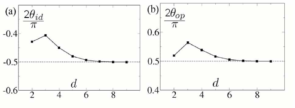
They are consistent with the statistics obtained from anyon fusion arguments[11]: Let us discuss on the up-spin band only. Consider a bound state of two of fluxons $f_{\frac{1}{2}\uparrow}$, and another bound state of two fluxons $f_{\frac{1}{2}\uparrow}$. Then each bound state carries charge 1 and flux $2\pi\sim 0$ and thus is a fermion. As a result the statistical phase between two $f_{\frac{1}{2}\uparrow}$ fluxons would be one-quarter of that of fermions, i.e. $\pm\frac{\pi}{4}$. By numerical calculation we find $\theta(f_{\frac{1}{2}\uparrow},f_{\frac{1}{2}\uparrow})=-\frac{\pi}{4}$. From particle-hole symmetry we immediately conclude that $\theta(f_{-\frac{1}{2}\uparrow},f_{-\frac{1}{2}\uparrow})=-\frac{\pi}{4}$, too. Now consider a bound state of an $f_{\frac{1}{2}\uparrow}$ fluxon and an $f_{-\frac{1}{2}\uparrow}$ fluxon. This bound state carries charge $0$ and should be a boson. This implies that $\theta(f_{\frac{1}{2}\uparrow},f_{-\frac{1}{2}\uparrow})=\frac{\pi}{4}$. $\theta(f_{\alpha_{1}\uparrow},f_{\alpha_{2}\uparrow})$ one can determine the statistical phase in the down-spin band $\theta(f_{\alpha_{1}\downarrow},f_{\alpha_{2}\downarrow})$ readily:

$$\theta(f_{\alpha_{1}\downarrow},f_{\alpha_{2}\downarrow})=-\theta(f_{\alpha_{1}\uparrow},f_{\alpha_{2}\uparrow}).$$ (4)

This is because the Hamiltonian for the down spin band is the hermitian conjugate of that for the up spin band. Given Fig.(3) and Eqs.(3,4) we have determined the quantum statistics of fluxons. The result is shown in the following Table. In general fluxons should experience a background magnetic field (the fermion density) as they hop around. However, since there are on average two fermions per site (see Fig.2(a)), this background magnetic flux is $2\pi$ per plaquette, hence is equivalent to no flux. The above results should be robust against perturbations so long as the bulk gap is preserved.

Self statistics	Mutual statistics
$c=\pm 1/2$	$c=\pm 1/2$
$\theta(f_{c\uparrow,c\downarrow},f_{c\uparrow,c\downarrow})=~~0$	$\theta(f_{c\uparrow,c\downarrow},f_{-c\uparrow,-c\downarrow})=0~~~~~~$ $\theta(f_{c\uparrow,c\downarrow},f_{c\uparrow,-c\downarrow})={\pi\over 2}$ $\theta(f_{c\uparrow,c\downarrow},f_{-c\uparrow,c\downarrow})={\pi\over 2}$
$\theta(f_{c\uparrow,-c\downarrow},f_{c\uparrow,-c\downarrow})=0$	$\theta(f_{c\uparrow,-c\downarrow},f_{-c\uparrow,c\downarrow})=0~~~~~~$ $\theta(f_{c\uparrow,-c\downarrow},f_{c\uparrow,c\downarrow})={\pi\over 2}$ $\theta(f_{c\uparrow,-c\downarrow},f_{-c\uparrow,-c\downarrow})={\pi\over 2}$

A new way to diagnose $Z_{2}$ TBI Note that the four fluxon states in Fig.1 are degenerate due to $T,PH_{\uparrow,\downarrow}.$ The degeneracy between the charged and neutral fluxon can be easily removed by adding a weak short range charge repulsion to the original fermion model. After that, one expects the lowest energy fluxons to be the neutral ones: $f_{+\frac{1}{2}\uparrow,-\frac{1}{2}\downarrow}$ and $f_{-\frac{1}{2}\uparrow,+\frac{1}{2}\downarrow}$. In the rest of the paper we refer to them as spin fluxons. The $S_{z}=\pm 1/2$ spin fluxons form a Kramer’s pair upon time reversal.

So far in our discussion $R_{S_{z}}$ is a symmetry of the Hamiltonian. This global $U(1)$ symmetry justifies the corresponding TBI to be called a $U(1)$ TBI. However, the presence of a Kramer pair of neutral fluxon is more general. We have checked that as long as $T$ is unbroken, each neutral fluxon always comes as a Kramer pair. This is true even after breaking $R_{S_{z}}$(by adding, say, T-invariant spin-flip hopping term to the TBI Hamiltonian[3]), and/or $PH_{\uparrow\downarrow}$ (by adding, say, a chemical potential term to the TBI Hamiltonian). This robust degeneracy allows one to diagnose the $T$-invariant TBI, or $Z_{2}$ TBI[3] without resorting to edge states. For example, consider a $Z_{2}$ TBI on a torus. One can introduce $2N$ far apart, low-energy, spin fluxons by, e.g., imposing an energy penalty for charge accumulation. The ground state will be $2^{2N}$-fold degenerate. On the other hand a trivial band insulator has no such degeneracy. Hence this degeneracy differentiates a $Z_{2}$ TBI from a trivial band insulator. This can be implemented as a numerical diagnosis of $Z_{2}$ TBIs.

This study naturally generalizes to three dimension. For the 3D-$Z_{2}$ insulator(which is refered as the strong topological insulator in literatures, for instance [4, 5]), we find for a closed $\pi$-flux loop, there are two gapless one-dimensional Dirac fermion modes propagating along the $\pi$-flux loop in opposite directions and are Kramers conjugates of each other.

Dynamical $\pi$-fluxes and TBI*  In order to make the fluxon elementary excitations, we give the $Z_{2}$ variable dynamics. This is achieved by adding the following term to Eq. (1).

$$H_{{\rm TBI}^{*}}=H_{0}-K\sum_{\square}\prod_{\langle ij\rangle\in\square}\tau_{ij}^{z}+J\sum_{\langle ij\rangle}\tau^{x}_{ij}.$$ (5)

The fermions $\Psi_{i,\sigma}$ in the above Hamiltonian carries a $Z_{2}$ gauge charge, hence are not ordinary electrons. We refer to such a correlated band insulator with emergent $Z_{2}$ gauge fields as a TBI*. Nonetheless, the fundamental fermion degrees of freedom of Eq. (5) possesses both the fermion number and the spin quantum number. In the following we show that the elementary excitations of this model exhibit separation of the the fermion quantum number (which we abbreviated by “chanrge”) and spin.

In Eq. (5) the term $\prod_{\langle ij\rangle\in\square}\tau_{ij}^{z}$ is the $Z_{2}$ gauge flux going through a plaquette, and $K,J$ are gauge couplings. The last term of Eq.(5) causes the fluxons to hop from one to a neighboring plaquette. As usual, $\tau^{x,z}$ are the first and third components of the Pauli matrices. The Hamiltonian in Eq.(5) has to be supplemented with a local constraint on every site (the ‘Gauss Law’) $\prod_{j\in{\rm n.n.of~}i}\tau_{ij}^{x}=(-1)^{\Psi_{i,\sigma}^{\dagger}\Psi_{i,\sigma}}$, where the product is over nearest neighbors of the site ‘i’. For $J=0$ the ground state of Eq.(1) lies in the gauge sector where there is no flux in any plaquette. Under that condition it is always possible to tune the parameters so that the fluxons are the lowest energy excitations in the fermionic sector. For non-zero $J$ the static fluxons are no longer eigen excitations. However, so long as the fluxon creation energy $>>J$ the delocalization of fluxons will not close the excitation gap. In that limit the gapped mobile fluxons exhibit spin-charge separation as illustrated in Fig.1.

Spin fluxon condensation In the rest of this paper we will assume the spin fluxons to be the lowest energy excitations. Now let us ask what happens as the magnitude of $J$ is increased. When the energy cost in creating a static spin fluxon is counter balanced by the kinetic energy gain due to its delocalization, spin fluxons will spontaneously proliferate. Owing to their Bose statistics this will trigger Bose condensation at zero temperature. It is interesting to ask what is the nature of the new ground state and what is the nature of the (quantum) phase transition. In the following we shall discuss two scenarios.

(I) If $S_{z}$ is conserved, two spin fluxons of opposite $S_{z}$ can be created and annihilated dynamically, while two fluxons with the same $S_{z}$ can not. In this case we can view the $S_{z}=-\frac{1}{2}$ fluxon as the anti-particle of $S_{z}=+\frac{1}{2}$ fluxon, and T transforms one into the other. The symmetry which dictates the $S_{z}$ conservation is $R_{S_{z}}$. Under such condition, the field theory describing the spin fluxon condensation is characterized by the following Lagrangian density

$$\mathcal{L}=\frac{1}{2}|\partial_{\tau}\phi|^{2}+\frac{1}{2}|\nabla\phi|^{2}+\frac{m^{2}}{2}|\phi|^{2}+\frac{1}{4!}u|\phi|^{4},$$ (6)

where $\phi$ is the complex fluxon field. The two phases of this field theory are: 1) the fluxon uncondensed phase where $\langle\phi\rangle=0$ and $R_{S_{z}}$ is unbroken. In this phase, creating a spin fluxon costs a finite energy. In the gauge theory jargon the $Z_{2}$ gauge field is in the deconfined phase. This is the phase of a spin liquid with a finite gap for spinon (bosonic) excitations. 2) The fluxon condensed phase where $\langle\phi\rangle\neq 0$ and $R_{S_{z}}$ is spontaneously broken. This is a phase where the $Z_{2}$ gauge field fluctuates so strongly that it confines the fermionic charge excitations. Magnetically it is an XY ordered ferromagnet. (We have implicitly assumed that the ordering is easy plane rather than easy axis, which is natural in the presence of spin-orbit coupling [15]) Moreover, since the fermionic charge excitation are absent at low energies throughout the transition, this phase is an electric insulator. Thus spin fluxon condensation triggers a spin liquid to a ferromagnetic insulator transition. According to Eq. (6), the universality class of the transition is 3D XY. The fact that $\phi$ transforms as $e^{i\theta/2}$ while the order parameter $S^{+}$ transform like $e^{i\theta}$ under $R_{S_{z}}$ implies the identification $S^{+}\sim\phi^{2}$. Hence, there is a subtle difference from the regular XY transition obtained from magnon condensation (i.e. condensing $S^{+}$ itself), in that the order parameter’s critical scaling dimension is anomalously large [13].

(II) $S_{z}$ is not conserved, but T is preserved. Now, one can add spin rotation breaking terms to the effective Lagrangian as long as they preserve time reversal symmetry. The first such term in the long wavelength limit is $g(S^{+})^{2}+{\rm h.c.}$, is actually a quartic term when written in terms of the spinon fields introduced above $g\phi^{4}+{\rm h.c.}$. Now, the condensation of $\phi$ leads to a confined insulator with the spontaneous breaking of time reversal symmetry. Interestingly, although such an insulator has an Ising order parameter, the transition is expected to remain 3D XY like, due to the irrelevance of four fold anisotropy at the XY critical point.

In the past, the transition to magnetically ordered states from spin liquids has been described using the Higgs mechanism. Here, we have described how confinement can also lead to magnetic order. This mechanism can lead to novel quantum phase transitions complementing those discussed in [14], which will be described in future work [15].