Light curves of five type Ia supernovae at intermediate redshiftThanks: Based on joint observations made through the Isaac Newton Groups’ Wide Field Camera Survey Programme with the Isaac Newton Telescope and the Jacobus Kapteyn Telescope operated on the island of La Palma by the Isaac Newton Group in the Spanish Observatorio del Roque de los Muchachos of the Instituto de Astrofisica de Canarias. Part of the data presented here have also been taken using ALFOSC, which is owned by the Instituto de Astrofisica de Andalucia (IAA) and operated at the Nordic Optical Telescope under agreement between IAA and the NBIfAFG of the Astronomical Observatory of Copenhagen.

Abstract

Aims. We present multi-band light curves and distances for five type Ia supernovae at intermediate redshifts, $0.18<z<0.27$.

Methods. Three telescopes on the Canary Island of La Palma, INT, NOT, and JKT, were used for discovery and follow-up of type Ia supernovae in the $g^{\prime}$ and $r^{\prime}$ filters. Supernova fluxes were measured by simultaneously fitting a supernova and host galaxy model to the data, and then calibrated using star catalogues from the Sloan Digital Sky Survey.

Results. The light curve shape and colour corrected peak luminosities are consistent with the expectations of a flat $\Lambda$CDM universe at the $1.5\sigma$ level. One supernova in the sample, SN1999dr, shows surprisingly large reddening, considering both that it is located at a significant distance from the core of its host ($\sim 4$ times the fitted exponential radius) and that the galaxy can be spectroscopically classified as early-type with no signs of ongoing star formation.

1 Introduction

Measurements of type Ia supernovae (SN Ia) have had a dramatic impact on the field of cosmology, and lead to the discovery of the acceleration of the Universe (Riess et al. (1998); Perlmutter et al. (1999)). Since then the number of well measured SN Ia:s has increased considerably through the joint effort of several independent research groups. However, the majority of the search campaigns have either been looking for high redshift SN Ia (Knop et al. (2003); Astier et al. (2006); Riess et al. (2007); Wood-Vasey et al. (2007) and references therein) where the difference in the relative luminosity distance between different cosmological models increases, as shown by Goobar & Perlmutter (1995), or low redshift SN Ia (Hamuy et al. (1996); Riess et al. (1999); Jha et al. (2006)) which are essential for both anchoring the Hubble diagram as well as learning more about SN Ia properties. With the exception of the ongoing three year Sloan Digital Sky Survey SN campaign initiated in 2005 (Frieman et al. (2008); Sako et al. (2008)), the redshift region around $z\sim 0.2$ in the Hubble diagram has not been heavily explored.

This missing link in the SN Ia Hubble diagram is of great importance as it corresponds to the epoch of dark energy domination. Thus it presents interesting opportunities for testing for a possible time evolution of the dark energy density with data-sets probably less plagued by systematic uncertainties. Effects such as SN Ia brightness evolution or gravitational lensing are expected to be much less than at higher redshifts.

The current best estimates of cosmological parameters from SNLS (Astier et al. (2006)) and ESSENCE (Wood-Vasey et al. (2007)) are approaching the systematic uncertainties for these projects. This further increases the need of a better understanding of SN Ia properties with the aim of calibrating them to even better precision.

Also, for these redshifts the rest frame ultraviolet region of the SN Ia spectrum has been redshifted into the visible wavelength area, illustrated in Figure 1, where the detector efficiency is higher and the atmosphere is transparent and less variable.

Figure 1: Overlap between rest frame $UBV$ (dashed) and observed, effective, INT $g^{\prime}$ and $r^{\prime}$ (solid) filters for the mean redshift, $z=0.22$, of the SN sample presented here. The dotted curve shows the normalised spectral template of a type Ia supernova (Nugent et al. (2002)) at maximum.

This is a part of the type Ia spectrum that contains a large fraction of the total flux, and it is therefore very important to understand the intrinsic UV-properties for interpreting high redshift data.

Furthermore, the UV part of the spectrum is of particular interest as it has been suggested that a redshift evolution of the SN Ia properties due to differences in the progenitor metallicity, if present, may be detectable in this wavelength region (Hoeflich et al. (1998); Lentz et al. (2000)). Intermediate redshift SNe are bright enough to allow high precision spectroscopy (Ellis et al. (2007)), and a large number of well observed SN Ia at these redshifts may very well turn out to be essential for understanding rest frame $U$-band properties.

To address these issues, a pilot campaign for photometric and spectroscopic follow-up of intermediate redshift SN Ia was launched in 1999. Here we present photometric follow-up of five SN Ia from the 1999 campaign. The spectra of these SNe have already been published in Balland et al. (2006).

In Sect. 2 we describe the search and the photometric follow-up. Sect. 3 covers the reduction and photometric measurements, followed by a description of the light curve analysis and possible systematic errors in Sect. 4. In Sect. 5 the results are summarised and discussed.

2 Search and Follow-up Observations

The search campaign was carried out during autumn 1999 as a piggy-back project of the Wide Field Survey (WFS) (McMahon et al. (2001)) at the Isaac Newton Telescope (INT). The WFS obtained multi-colour data in the broad band, $u^{\prime}$, $g^{\prime}$, $r^{\prime}$, $i^{\prime}$, $z^{\prime}$ filter set during 1998–2003, covering 200 square degrees with a depth of $r^{\prime}\approx 24$ and $g^{\prime}\approx 25$. The Wide Field Camera (WFC), with four 4k$\times$2k CCDs and a total field of view of $0.27$ square degrees, was used and the $g^{\prime}$ and $r^{\prime}$ data was obtained repeatedly with a cadence particularly suitable for finding SNe around maximum (Perlmutter et al. (1995), 1997).

The SNe presented here were discovered by seeing-matching and comparing two WFS data sets in the $g^{\prime}$-band. The first set was observed in mid August 1999 and the second roughly one month later. The August data consisted of 600 s exposures, while two 240 s frames were obtained for the same fields in September 1999. Altogether, three subtractions were made by both considering the September discovery images individually, and by using their coadded sum. Candidates were then selected by requiring detection within 2 pixels on all three frames in order to efficiently reject cosmic rays and fast-moving objects. In addition to this, a flux increase within one FWHM seeing radius of at least 15 % was used as a search criteria. The candidates were re-observed 1–2 days later and rejected unless the above criteria were still fulfilled. This excluded possible slow-moving objects from the candidate sample. The whole search resulted in a total of 15 SN candidates.

Spectroscopy of the candidates was obtained using the red channel of the ISIS instrument on the 4.2 m William Herschel Telescope. Additional spectroscopy was obtained for two of the candidates, (1999du and 1999dv), using the 2.5 m Nordic Optical Telescope (NOT) three weeks after discovery. Ten of the SNe, shown in Table 1 with their approximate discovery magnitude and spectroscopic redshifts, were confirmed as SN Ia (Balland et al. (2006)).

Table 1: The ten SN Ia discovered in the autumn 1999 campaign.

	SN	$\alpha\ (2000)$	$\delta\ (2000)$	$g^{\prime}$	$z$
$\rightarrow$	1999dr	23 00 17.56	$-$00 05 12.5	22.1	0.178
	1999dt	00 45 42.29	$+$00 03 22.2	23.5	0.437
$\rightarrow$	1999du	01 07 05.94	$-$00 07 53.8	22.8	0.260
$\rightarrow$	1999dv	01 08 58.96	$+$00 00 24.8	21.8	0.186
	1999dw	01 22 52.80	$-$00 16 20.8	24.1	0.460
$\rightarrow$	1999dx	01 33 59.45	$+$00 04 15.3	22.2	0.269
$\rightarrow$	1999dy	01 35 49.53	$+$00 08 38.3	21.7	0.215
	1999dz	01 37 03.24	$+$00 01 57.9	23.4	0.486
	1999ea	01 47 26.09	$-$00 02 07.2	23.3	0.397
	1999gx	00 34 15.47	$+$00 04 26.2	23.3	0.493

The redshifts could be determined from host galaxy features for all SNe and the precision of these measurements is typically 0.001.

Five of the SN Ia had redshifts below $z<0.3$, marked with arrows in Table 1, and were all discovered before or around maximum. For these, photometric follow-up in the $g^{\prime}$ and $r^{\prime}$ bands was carried out using the ALFOSC instrument on the 2.5 m NOT and the SITe2 CCD camera on the 1.0 m Jacobus Kapteyn Telescope (JKT) in addition to INT. This filter combination corresponds approximately to rest frame $UBV$ for $z\sim 0.2$. For the remaining SNe ($z>0.3$), we do not have any photometric follow-up.

SN-free reference images of the host galaxies were obtained approximately one year after discovery with INT in both $g^{\prime}$ and $r^{\prime}$.

3 Reduction and Photometry

The INT images were reduced using the WFS pipeline (Irwin & Lewis (2001)). For the NOT and JKT images, standard reduction including bias subtraction and flat fielding, was carried out using the IRAF software. A spatially varying multiplicative factor was still present for the JKT images after flat fielding, which possibly could originate from small filter movements during the night. The effect was corrected for by fitting a smooth surface to each image. Some images showed signs of bad telescope tracking and were rejected.

3.1 Photometry

The photometry technique applied for this data set is based on the same method (Fabbro (2001)) used for the latest SNLS data release (Astier et al. (2006)).

For each exposure covering a given SN, the SExtractor package (Bertin & Arnouts (1996)) was first used to create object catalogues. These were used to fit geometric transformations to the best seeing photometric reference image of the sample and all other images were then re-sampled to this frame. In order to properly compare images obtained during different seeing conditions we fitted convolution kernels, modelled by a linear decomposition of Gaussian and polynomial basis functions (Alard & Lupton (1998); Alard (2000)), between the photometric reference and each of the remaining images for the given passband. The kernels were fitted by using image patches centred on objects across the field. The quality of both the geometric transformations and the fitted kernels was investigated by carrying out image subtractions and searching for residual artifacts. Such artifacts were in general absent and had minimal impact on the SN photometry.

For a small area centred on an SN, the PSF is not expected to have any spatial variation. A time series of such patches, $I_{i}$, can be described by the following model

$$I_{i}(x,y)=f_{i}\cdot\left[K_{i}\otimes\mathrm{PSF}\right](x-x_{0},y-y_{0})+\left[K_{i}\otimes G\right](x,y)\,+S_{i}\,.$$

Here, $I_{i}(x,y)$ is the value in pixel $(x,y)$ of image $i$, $f_{i}$ is the SN flux, PSF is the point spread function for the photometric reference, $K_{i}$ is the kernel between the reference and image $i$, $\otimes$ is the convolution operator, $(x_{0},y_{0})$ is the SN-position, $G$ is a time independent galaxy model and $S_{i}$ is the local sky background.

The PSF was obtained from the field stars on the photometric reference image. An initial guess of the SN-position was found by stacking all images that were believed to contain SN-light and subtracting the stack of SN-free reference images from this. The parameters of the model, $f_{i}$, $x_{0}$, $y_{0}$, $G$ and $S_{i}$ were then simultaneously fitted to the whole patch set by minimising

$$\chi^{2}=\sum_{i}^{N}\sum_{x,y}^{k,n}W_{i}(x,y)\cdot\left[D_{i}(x,y)-I_{i}(x,y)\right]^{2}\,,$$

where $D_{i}(x,y)$ is the data value in pixel $(x,y)$ on image patch $i$ and $W_{i}(x,y)$ is the weight. The Poisson and read-out noise as well as kernel and PSF uncertainties were propagated to $W_{i}$. The sums were carried out over the total number of image patches, $N$, and the patch dimensions, $k\times n$. In this work, we used a non-analytic host galaxy model with one parameter for each pixel. This means that the model is degenerate with the SN and in order to break this degeneracy we kept $f_{i}=0$ fixed for the SN-free INT images obtained in 2000. The model is also degenerate with the local sky background, $S_{i}$, that needs to be fixed to zero on one image. The total number of fitting parameters will then add up to: $N-R$ SN fluxes where $R$ is the number of SN-free images, $k\cdot n$ for the time-independent galaxy model, $N-1$ sky values, and 2 for the SN position, i.e. $1+2N-R+k\cdot n$.

An example of image, galaxy model residuals, together with the resulting residuals when the full model has been subtracted, can be seen in Figure 2 for increasing epochs. Here the profile residual plots show the deviation from zero in standard deviations vs the distance from the SN position in pixels. The last row of the plot shows the SN-free epoch, obtained approximately one year after discovery. Different patch sizes reflect the differences in image quality where a small patch size represents good seeing conditions.

Figure 2: A sample of patches for increasing epochs from the $g^{\prime}$ (left column) and $r^{\prime}$-band (right column) light curve builds of 1999du. Each triplet represent first the untouched data patch, the galaxy model subtracted data patch, and a profile plot where the full galaxy $+$ PSF model has been subtracted from the data patch. The profile plot shows the deviation from zero in standard deviations vs the distance from the SN position in pixels. The last row of the plot shows the SN-free epoch, obtained approximately one year after discovery. The different patch sizes reflect the differences in image quality. A small patch size represents good seeing conditions.

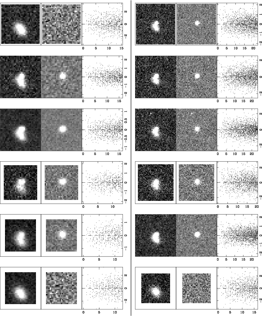
The fitted SN-fluxes are presented in Table 2, and the corresponding instrumental magnitudes in the INT system can be obtained as $m_{\mathrm{INT}}=-2.5\log_{10}f+ZP_{AB}$, where $f$ and the $ZP_{AB}$ is the flux and AB zero point from the table. This table also shows the image quality (I.Q.) of each epoch and is defined as the FWHM in arc seconds of a point source. 2

Table 2: Follow-up photometry of the five SNe presented in this work.

SN	MJD	Tel.	Exp. time	Band	Flux		$ZP_{AB}$	I.Q.
1999dr	$51399.98$	INT	599	$g^{\prime}$	1661	(360)	31.80 (0.02)	2.00
1999dr	$51422.99$	INT	638	$g^{\prime}$	6775	(366)	31.80 (0.02)	1.30
1999dr	$51423.99$	INT	239	$g^{\prime}$	6285	(408)	31.80 (0.02)	1.20
1999dr	$51427.06$	INT	599	$g^{\prime}$	4245	(277)	31.80 (0.02)	1.20
1999dr	$51430.93$	INT	599	$g^{\prime}$	2755	(238)	31.80 (0.02)	1.20
1999dr	$51430.93$	INT	599	$r^{\prime}$	7771	(503)	31.64 (0.02)	1.00
1999dr	$51434.99$	JKT	1800	$r^{\prime}$	4082	(15001)	31.64 (0.02)	2.40
1999dr	$51435.09$	JKT	5400	$g^{\prime}$	1437	(510)	31.80 (0.02)	2.50
1999dr	$51435.97$	JKT	5400	$g^{\prime}$	1989	(258)	31.80 (0.02)	1.20
1999dr	$51436.90$	JKT	5400	$r^{\prime}$	6056	(1412)	31.64 (0.02)	2.40
1999dr	$51454.89$	JKT	977	$r^{\prime}$	2450	(769)	31.64 (0.02)	1.00
1999dr	$51454.99$	INT	2396	$g^{\prime}$	638	(127)	31.80 (0.02)	1.70
1999dr	$51455.07$	INT	3595	$r^{\prime}$	2403	(373)	31.64 (0.02)	2.10
1999dr	$51455.90$	INT	599	$r^{\prime}$	2253	(361)	31.64 (0.02)	1.00
1999dr	$51456.02$	JKT	3600	$g^{\prime}$	1030	(246)	31.80 (0.02)	1.00
1999dr	$51456.90$	JKT	5400	$r^{\prime}$	2272	(598)	31.64 (0.02)	1.50
1999dr	$51457.89$	JKT	3600	$r^{\prime}$	2218	(655)	31.64 (0.02)	1.50
1999dr	$51458.90$	JKT	3600	$g^{\prime}$	681	(565)	31.80 (0.02)	2.10
1999du	$51429.16$	INT	479	$g^{\prime}$	8018	(404)	32.00 (0.02)	1.00
1999du	$51431.09$	INT	599	$g^{\prime}$	11757	(493)	32.00 (0.02)	1.10
1999du	$51431.10$	INT	599	$r^{\prime}$	23228	(1820)	32.78 (0.02)	1.10
1999du	$51437.06$	JKT	5400	$g^{\prime}$	20052	(1227)	32.00 (0.02)	2.00
1999du	$51438.05$	JKT	5400	$r^{\prime}$	40797	(2884)	32.78 (0.02)	1.30
1999du	$51452.92$	NOT	3600	$g^{\prime}$	15038	(566)	32.00 (0.02)	1.20
1999du	$51452.96$	NOT	3000	$r^{\prime}$	37554	(2150)	32.78 (0.02)	1.00
1999du	$51454.93$	NOT	3600	$r^{\prime}$	36857	(2108)	32.78 (0.02)	1.30
1999du	$51454.97$	NOT	3000	$g^{\prime}$	13266	(531)	32.00 (0.02)	1.50
1999du	$51456.06$	INT	1798	$r^{\prime}$	36466	(2055)	32.78 (0.02)	1.20
1999du	$51456.07$	INT	1798	$g^{\prime}$	12400	(478)	32.00 (0.02)	1.30
1999du	$51456.98$	JKT	5400	$g^{\prime}$	12676	(747)	32.00 (0.02)	1.70
1999du	$51457.05$	JKT	4400	$r^{\prime}$	33045	(2491)	32.78 (0.02)	1.40
1999du	$51458.06$	INT	1198	$r^{\prime}$	33341	(2022)	32.78 (0.02)	1.10
1999du	$51458.07$	INT	1198	$g^{\prime}$	10831	(453)	32.00 (0.02)	1.10
1999du	$51459.10$	JKT	2216	$r^{\prime}$	28781	(4618)	32.78 (0.02)	2.50
1999du	$51461.06$	INT	599	$r^{\prime}$	27689	(1962)	32.78 (0.02)	1.30
1999du	$51461.07$	INT	599	$g^{\prime}$	8301	(409)	32.00 (0.02)	1.40
1999du	$51597.99$	NOT	600	$g^{\prime}$	13775	(722)	32.00 (0.02)	1.70
1999dv	$51430.09$	INT	479	$g^{\prime}$	50185	(2195)	33.00 (0.02)	1.20
1999dv	$51431.12$	INT	599	$r^{\prime}$	43118	(1880)	32.76 (0.02)	1.00
1999dv	$51431.18$	INT	599	$g^{\prime}$	57484	(2280)	33.00 (0.02)	1.00
1999dv	$51436.07$	JKT	3600	$g^{\prime}$	80463	(3304)	33.00 (0.02)	1.10
1999dv	$51436.12$	JKT	3600	$r^{\prime}$	61249	(2799)	32.76 (0.02)	1.10
1999dv	$51453.06$	NOT	2400	$r^{\prime}$	47881	(2075)	32.76 (0.02)	1.20
1999dv	$51454.11$	JKT	3600	$r^{\prime}$	48940	(3096)	32.76 (0.02)	1.40
1999dv	$51455.02$	NOT	3000	$g^{\prime}$	30991	(1563)	33.00 (0.02)	1.50
1999dv	$51455.07$	NOT	3600	$r^{\prime}$	42884	(1837)	32.76 (0.02)	1.30
1999dv	$51456.10$	INT	598	$r^{\prime}$	42163	(2058)	32.76 (0.02)	1.00
1999dv	$51457.13$	JKT	5400	$g^{\prime}$	25043	(1941)	33.00 (0.02)	1.20
1999dv	$51458.08$	INT	1198	$r^{\prime}$	37552	(1674)	32.76 (0.02)	1.10
1999dv	$51458.10$	INT	1198	$g^{\prime}$	23604	(1313)	33.00 (0.02)	1.30
1999dv	$51458.97$	JKT	3600	$r^{\prime}$	31942	(4161)	32.76 (0.02)	2.30
1999dv	$51461.10$	INT	599	$r^{\prime}$	32740	(1666)	32.76 (0.02)	1.30
1999dv	$51461.11$	INT	599	$g^{\prime}$	16803	(1174)	33.00 (0.02)	1.20
1999dx	$51429.21$	INT	239	$g^{\prime}$	10353	(592)	31.97 (0.02)	1.00
1999dx	$51431.20$	INT	599	$g^{\prime}$	11994	(566)	31.97 (0.02)	1.00
1999dx	$51437.18$	JKT	6102	$g^{\prime}$	10953	(1035)	31.97 (0.02)	2.20
1999dx	$51438.13$	JKT	5400	$r^{\prime}$	28422	(2266)	32.79 (0.02)	1.30
1999dx	$51453.11$	NOT	3600	$g^{\prime}$	2271	(296)	31.97 (0.02)	1.00
1999dx	$51453.25$	NOT	600	$r^{\prime}$	22849	(6849)	32.79 (0.02)	1.60
1999dx	$51455.13$	NOT	3000	$r^{\prime}$	10323	(1429)	32.79 (0.02)	1.10
1999dx	$51455.17$	NOT	3600	$g^{\prime}$	1925	(262)	31.97 (0.02)	1.30
1999dx	$51456.11$	JKT	1800	$g^{\prime}$	2595	(599)	31.97 (0.02)	1.00
1999dx	$51456.16$	INT	599	$r^{\prime}$	12182	(1537)	32.79 (0.02)	1.20
1999dx	$51457.05$	INT	1198	$g^{\prime}$	1718	(252)	31.97 (0.02)	1.10
1999dx	$51457.07$	INT	1198	$r^{\prime}$	10063	(1097)	32.79 (0.02)	1.00
1999dx	$51457.96$	JKT	5400	$r^{\prime}$	10326	(1844)	32.79 (0.02)	1.30
1999dx	$51458.04$	JKT	3600	$g^{\prime}$	1464	(474)	31.97 (0.02)	1.40
1999dx	$51462.12$	INT	599	$g^{\prime}$	1280	(281)	31.97 (0.02)	1.50
1999dx	$51462.12$	INT	598	$r^{\prime}$	8180	(1544)	32.79 (0.02)	1.60
1999dy	$51429.20$	INT	479	$g^{\prime}$	19205	(751)	31.82 (0.02)	1.00
1999dy	$51431.20$	INT	599	$g^{\prime}$	22519	(818)	31.82 (0.02)	0.90
1999dy	$51438.18$	JKT	1800	$g^{\prime}$	25252	(1262)	31.82 (0.02)	1.30
1999dy	$51438.23$	JKT	2400	$r^{\prime}$	88645	(4827)	33.18 (0.02)	1.50
1999dy	$51453.20$	NOT	2400	$g^{\prime}$	12378	(720)	31.82 (0.02)	1.70
1999dy	$51453.22$	NOT	2400	$r^{\prime}$	56868	(2790)	33.18 (0.02)	1.40
1999dy	$51454.99$	JKT	1800	$r^{\prime}$	56156	(4367)	33.18 (0.02)	1.70
1999dy	$51455.22$	NOT	3600	$g^{\prime}$	10136	(531)	31.82 (0.02)	1.60
1999dy	$51455.25$	NOT	600	$r^{\prime}$	50133	(3401)	33.18 (0.02)	1.50
1999dy	$51456.15$	JKT	3600	$g^{\prime}$	9185	(657)	31.82 (0.02)	1.30
1999dy	$51456.18$	INT	599	$r^{\prime}$	50905	(2564)	33.18 (0.02)	1.20
1999dy	$51458.11$	JKT	1800	$r^{\prime}$	48287	(5086)	33.18 (0.02)	1.80
1999dy	$51458.16$	JKT	1800	$g^{\prime}$	7374	(1599)	31.82 (0.02)	2.60

When multiple exposures are available for a given night, the measured SN fluxes are compared to each other in order to make sure that they agree within their statistical uncertainty. This was the case for all nights except for the 1999dx $g^{\prime}$ exposures from 1999-09-08 where, after a more careful investigation, it was concluded that one of the exposures was plagued with a cosmic ray very close to the SN, and the image was therefore excluded.

3.2 Subtraction Precision

In order to test the robustness of the photometric method and check for systematic errors, the fitted SN + galaxy model was subtracted from each data patch. Possible subtraction and galaxy model errors were explored both by measuring the residual flux within one FWHM aperture radius on the subtractions, and by studying how the fitted SN-fluxes of any given epoch is changing as more epochs are added to the fit. These tests did not result in any deviations exceeding the statistical expectations.

3.3 Calibration

All fitted SN fluxes from the method described above are by construction tied to the normalisation of the fitted PSF of the photometric reference image. In order to calibrate the SN photometry it is therefore necessary to determine the zero point that relates this normalisation to a standard photometric system. For this purpose we used the field stars in the images as tertiary standard stars. The instrumental magnitudes of these objects were measured using the exact same procedure as for the SNe except no host galaxy models were fitted.

In principle, the magnitudes of the tertiary standard stars could be determined from observations of standard stars during the nights. However, since that data was not always available, and in order to obtain a consistent calibration for all SNe, we decided to use photometric catalogues of our fields from the Sloan Digital Sky Survey (SDSS) DR4 (Adelman-McCarthy et al. (2006)), and tie our calibration to their photometric system (Fukugita et al. (1996)), which for $g^{\prime}$ and $r^{\prime}$ is very close to the standard AB system (Oke & Gunn (1983)). From the SDSS catalogues we chose to use PSF magnitudes and converted them from SDSS magnitudes (Lupton et al. (1999)) to standard Pogson magnitudes (Pogson, (1856)).

Since the INT data dominates the sample, and since we only had SN-free reference images obtained with this telescope, we consistently chose to use this as our natural magnitude system. Systematic effects on NOT and JKT points due to this are discussed below. Zero points were then determined by simultaneously fitting the following relation between our instrumental magnitudes, $m_{j}$, and the SDSS magnitudes, $m^{\mathrm{SDSS}}_{j}$, to all INT images for a given filter

$$\Delta m\equiv m_{j}-m^{\mathrm{SDSS}}_{j}=zp_{i}+c_{X}\cdot(g_{j}-r_{j})^{\mathrm{SDSS}}\,.$$ (1)

Here $zp_{i}$ is the zero point for image $i$, $c_{X}$ is the colour term for filter $X$, and $(g^{\prime}_{j}-r^{\prime}_{j})^{\mathrm{SDSS}}$ is the SDSS $g^{\prime}-r^{\prime}$ colour of the star $j$. The fit was carried out simultaneously in two iterations, using a 3$\sigma$ outlier rejection cut.

Both the zero points of the individual images and the common colour terms were obtained this way. The results and the number of stars used for the fits are presented in Table 3 and the first row of Table 4. The simultaneous fit for the $g^{\prime}$ band is also presented Figure 3, where $\Delta m$ denotes the difference between the measured instrumental magnitude and the SDSS magnitude. From this the individually fitted zero points have been subtracted in order to put all data points on the same scale and the magnitude differences are then plotted against the SDSS colours of the stars. Different plotting symbols represent different SN-fields, and the solid line shows the best fitted colour term for the sample. The RMS around the best fitted line is 0.05 mag. The reduced $\chi^{2}$ for the fits were $\chi^{2}/dof=1.06$ for $g^{\prime}$ and $\chi^{2}/dof=1.13$ for $r^{\prime}$. We chose to scale the error bars for each individual fit to match $\chi^{2}/dof=1.0$. We add an additional $0.01$ mag in quadrature to the fitted zero point uncertainties in order to account for the uncertainty of the SDSS zero points. In these fits we observe a correlation between the zero points and the colour terms of $\rho\sim-0.6$.

Table 3: Simultaneously fitted zero points.

SN	$g^{\prime}$	$n_{g}$	$r^{\prime}$	$n_{r}$
1999dr	$31.78\pm 0.01$	85	$31.63\pm 0.01$	28
1999du	$31.98\pm 0.01$	51	$32.77\pm 0.01$	27
1999dv	$32.98\pm 0.01$	49	$32.76\pm 0.01$	59
1999dx	$31.95\pm 0.01$	26	$32.79\pm 0.01$	35
1999dy	$31.80\pm 0.01$	47	$33.18\pm 0.01$	43

Table 4: Measured colour terms for INT, NOT, and JKT.

Tel.	$g^{\prime}$	$r^{\prime}$
INT	$0.15\pm 0.01$	$-0.01\pm 0.01$
NOT	$0.11\pm 0.02$	$0.02\pm 0.01$
JKT	$0.15\pm 0.02$	$0.02\pm 0.01$

Figure 3: Fitted zero point solution in the INT $g^{\prime}$-band.

Note that the zero point is in this case the sum of three components; the instrumental zero point, the aperture correction to the PSF normalisation radius and the atmospheric extinction for the given airmass. We are also assuming that the atmospheric extinction is colour independent, an assumption that was further justified by studying the residuals for the individual image catalogues. We examined these residuals carefully for any brightness, colour, or position dependent correlations. Minor trends with CCD position could be detected at the edges of the detector, but these did not affect the overall calibration.

The fitted zero point solutions derived above can then be used together with colour information to obtain the standard magnitudes of other objects in the field. However, for SN-photometry the colour term corrections derived from stellar photometry is not applicable. This is due to the significant differences between SN and stellar spectral energy distributions (SED), and will lead to systematic errors (Stritzinger et al. (2002), Krisciunas et al. (2003)). For SN-photometry, it is therefore often more reliable to calculate the SED-dependent correction, $S$-correction, using synthetic photometry although this requires good knowledge of both the filter responses, the SED, and the zero point of the instrumental filter system.

The calibrated magnitude in any filter system, $X^{\prime}$, can be expressed as $m_{X^{\prime}}=-2.5\log_{10}(f)+ZP^{\prime}$, where $f$ is the measured flux and $ZP^{\prime}$ is the zero point for that system. The AB magnitude in the filter system $X$ can then be expressed as $m_{X}=m_{X^{\prime}}+S_{XX^{\prime}}$, where $S_{XX^{\prime}}$,

$$S_{XX^{\prime}}=-2.5\log_{10}\left(\frac{\int\lambda f_{\lambda}X_{\lambda}\,d\lambda}{\int\lambda f_{\lambda}X^{\prime}_{\lambda}\,d\lambda}\right)+2.5\log_{10}\left(\frac{\int(X_{\lambda}/\lambda)\,d\lambda}{\int(X^{\prime}_{\lambda}/\lambda)\,d\lambda}\right)\,,$$ (2)

is the above mentioned $S$-correction, $f_{\lambda}$ is the object SED and $X_{\lambda}$ and $X^{\prime}_{\lambda}$ are the filter responses of the two systems respectively. In equation (1) we approximated $S_{XX^{\prime}}$ as

$$S_{XX^{\prime}}\approx b+c_{X}\cdot(g_{j}-r_{j})^{\mathrm{SDSS}}\,,$$

dropping higher order terms. The zero point of the INT system, $ZP^{\prime}$ can then be expressed as $ZP^{\prime}=zp-b$, where $zp$ was fitted above, and $b$ remains to be determined. This constant does depend on the filter responses, but it is independent of the object SED. Therefore we could fit it by taking the $g^{\prime}$ and $r^{\prime}$ magnitudes for 14 photometric standard stars (Smith et al. (2002)) with colours $g^{\prime}-r^{\prime}<1.0$ that also have spectro-photometry (Stritzinger et al. (2005)) allowing calculation of $S_{XX^{\prime}}$ using equation (2). The result of these fits are shown in Table 5 and Figure 4.

Table 5: Fitted colour terms and $S$-correction filter offsets for INT.

Filter	$b$	$c_{X}$
$g^{\prime}$	$-0.014\pm 0.001$	$0.147\pm 0.003$
$r^{\prime}$	$-0.005\pm 0.001$	$0.010\pm 0.001$

Figure 4: Fitted linear relations for the synthetically calculated $S$-corrections in the $r^{\prime}$ (upper panel) and $g^{\prime}$ (lower panel) bands.

From the simultaneously fitted zero points in equation (1) together with the filter offsets in the first column of Table 5, the zero points in the INT system, $ZP^{\prime}$ can then be calculated for each photometric reference. These are presented in Table 2.

3.4 Instrument Wavelength Response

Since no SN-free reference images were obtained with neither NOT nor JKT, the INT references had to be used for constraining the host galaxy models for these images as well. Differences in the combined filter and instrument wavelength response between different instruments can be expected and are to some extent included in the uncertainties of the fitted kernels. However, it cannot be excluded that the fitted SN-fluxes could be biased when data from different instruments are brought into the fit. Calculating the impact of this potential systematic effect is difficult, but a rough estimate can be obtained by studying the similarities of the effective filter response between the different instruments. In order to do this we repeated the recipe from the calibration, using equation (1) together with JKT and NOT data and fitted the colour terms for these filters. The results are presented along with the INT values in Table 4.

Fortunately the colour terms for the three instruments are similar which suggests that the systematic error for this particular case can be expected to be small. We assumed a systematic uncertainty of 0.015 mag for all JKT and NOT points to account for it.

We further investigated the impact of the JKT and NOT data on the global fit by comparing the results when the whole data set was used with light curves exclusively built from INT data. The results from these two sets did not differ and therefore it can be concluded that the JKT and NOT data did not have any systematic effect on the host galaxy model fit.

Since the calibration was tied to the INT system we consistently chose to use the INT WFC effective filter response functions, provided by the Isaac Newton Group, for light curve fitting and $K$-corrections. Any wavelength dependent difference between these response function and the actual effective response of the system could introduce systematics into the analysis. However, since the synthetic calculations of the effective colour terms presented in Table 5 are in good agreement with the corresponding measured values in Table 4 it can be concluded that any systematics introduced by possible incorrect response functions are negligible.

4 Data Analysis

4.1 Light Curve Fitting

When SN Ia data is used for measuring cosmology, different correlated properties of the SN light curve is used in combination as a standard candle. Intrinsically brighter SN Ia are typically bluer and have a slower decline rate than intrinsically fainter objects (Phillips (1993)). Several different methods of combining the measured data to a single distance dependent property have been suggested (Goldhaber et al. (2001); Wang et al. (2003); Guy et al. (2005); Jha et al. (2007)).

For this work we chose the SALT2 method (Guy et al. (2007)) to fit the light curves. In summary, SALT2 consists of three components; a model of the time dependent average SN Ia SED, light curve shape variation from the average, and a wavelength dependent function that warps the SED. Variation from the average SED is parametrised by a single light curve shape parameter, $x_{1}$, chosen so that $x_{1}=0$ corresponds to the average decline rate, and $x_{1}<0$ and $x_{1}>0$ represents fast and slow decline rates respectively. The deviation, $c$, from the mean SN Ia $B-V$ colour at the time of $B$-band maximum is used to parameterise the contribution of the warping function. These two parameters are fitted for each SN together with the overall flux normalisation of the light curve $x_{0}$, which is related to the peak $B$-band magnitude, and the time of the $B$-band maximum. The fit is carried out in the observer instrumental frame rather than the standard rest frame. $K$-corrections are therefore built in to the fitting procedure which is a reasonable approach since they depend on the SED of the SN.

The model itself has been derived using both photometric and spectroscopic data from mainly the SNLS project, and is particularly well suited for the data set presented here since high redshift spectroscopy of the rest frame $U$-band has been used to ”train” the model.

The light curve data is corrected for Milky Way extinction using the Schlegel et al. (1998) dust maps and the extinction law from Cardelli et al. (1989) with $R_{V}=3.1$. Also the covariance matrices obtained from the simultaneous $\chi^{2}$-fit of the SN-fluxes are taken into consideration for the light curve fitting after the uncertainties of the fitted zero points are added as correlated errors. During the fit SALT2 can optionally update the weight matrices to take uncertainties of the model and cross filter $K$-corrections into account. In Table 6 we quote the fit results when both of these error sources were considered. The lightcurve shape, $x_{1}$, and colour, $c$, corrected peak $B$-band magnitude, $m^{\mathrm{eff}}_{B}$, is obtained as $m^{\mathrm{eff}}_{B}=m_{B}+\alpha_{x}\cdot x_{1}-\beta\cdot c$, where the values $\alpha_{x}=0.13\pm 0.01$ and $\beta=1.77\pm 0.16$ (Guy et al. (2007)) are used.

The best fitted light curves are shown together with the data in Figure 5. The stretch-colour corrected peak magnitudes, $m^{\mathrm{eff}}_{B}$, are further compared to the corresponding predictions for a $\Lambda$CDM universe in Figure 6. Predictions for dark energy models with an equation state parameter, $w$, differing from $w=-1$ have been plotted as well.

Figure 5: Light curve fits in $g^{\prime}$ (left column) and $r^{\prime}$ (middle column), showing normalised flux against the number of days, in the observer frame, since the time of fitted $B$-band maximum. The residual plots show the magnitude offset between the fitted light curve and the data from INT (triangle), NOT (circle) and JKT (square). The right column shows INT patches (13.2”$\times$13.2”) in the $g^{\prime}$ band centred on the SN.

Table 6: Light curve fit results using SALT2. The light curve stretch is calculated from $x_{1}$ using the relation derived in Guy et al. (2007).

SN	$\mathrm{MJD}_{\mathrm{max}}$	$m^{\mathrm{eff}}_{B}$	$m_{B}$	$c$	$x_{1}$	$s$	$\chi^{2}/dof$	$dof$
1999dr	$51413.28\pm 0.76$	$20.48\pm 0.21$	$21.59\pm 0.12$	$0.49\pm 0.09$	$-1.862\pm 0.450$	$0.826\pm 0.038$	$0.47$	$14$
1999du	$51444.15\pm 0.17$	$21.49\pm 0.10$	$21.30\pm 0.04$	$-0.03\pm 0.05$	$1.102\pm 0.295$	$1.083\pm 0.028$	$0.90$	$14$
1999dv	$51439.89\pm 0.11$	$20.50\pm 0.09$	$20.79\pm 0.03$	$0.10\pm 0.04$	$-0.773\pm 0.188$	$0.912\pm 0.017$	$1.39$	$12$
1999dx	$51434.45\pm 0.79$	$21.51\pm 0.16$	$21.81\pm 0.05$	$0.06\pm 0.08$	$-1.511\pm 0.513$	$0.852\pm 0.044$	$0.79$	$12$
1999dy	$51438.72\pm 0.21$	$21.08\pm 0.09$	$20.94\pm 0.03$	$-0.02\pm 0.05$	$0.743\pm 0.264$	$1.049\pm 0.025$	$0.57$	$9$

Figure 6: Residuals from the Hubble diagram where a $(\Omega_{M},\Omega_{\Lambda},w,M_{B}(h_{70}))=(0.26,0.74,-1,-19.31)$ cosmology (Astier et al. (2006)) has been subtracted from the third column ($m_{B}^{\mathrm{eff}}$) of Table 6. The outer error bars were obtained by adding an assumed intrinsic uncertainty of 0.13 mag in quadrature to the tabulated uncertainties. The dotted lines show the the predicted Hubble diagrams for different values of $w$.

4.1.1 Colour correction uncertainties

Throughout this work, we have adopted the SALT2 technique for light curve shape and colour corrections. This involves using an empirical colour correction factor, $\beta$, which if associated with reddening by dust along the line of sight, corresponds to the total selective extinction coefficient $\beta=R_{V}+1$. However, the best fit value, $\beta=1.77\pm 0.16$ (Guy et al. (2007)) is inconsistent with Milky Way dust properties ($R_{V}=3.1$). Thus, either the measured reddening indicates dust properties in the SN hosts which are quite different from Galactic dust, or that the measured colours are dominated by intrinsic SN variations, e.g. Nobili & Goobar (2008) find an average of $R_{V}=1.75\pm 0.27$ for a sample of near-by SNe but only $R_{V}\sim 1$ for a low reddening subset of the data

The assumptions on reddening law or circumstellar dust are particular important for one of the SNe, 1999dr. The implications are further discussed in the next section.

5 Discussion

The five intermediate-z SNe in our sample are well fitted by SALT2, as shown in Figure 5 and Table 6 for different SNe when the model errors are introduced. These appear to account for the light curve shape diversities that remain after stretch and colour warp has been considered. The average reduced $\chi^{2}$ of the sample is $\sim 0.81$.

The fitted light curve parameters all fall within the ’’normal’’ SN Ia range, with the exception of the colour of 1999dr, that suggests significant reddening. An extinction of this magnitude is unexpected both since the SN is located in the outer rim of the presumed host galaxy and since the host spectrum (Balland et al. (2006)) does not show any signs of star formation (see Table 7) which is usually associated with a dusty environment.

Table 7: Quoted host galaxy types from our spectroscopic classification in Balland et al. (2006).

SN	Host Type	Comment
1999dr	Sa/Sb	No emission
1999du	Sc/Starburst	Clear ident. Sc
1999dv	Sc/Starburst	Poor gal. signal
1999dx	E/S0	Emission lines
1999dy	Sc/Starburst	Faint

However, it should be pointed out that we lack data around maximum for this SN and the first $r^{\prime}$-band data point was obtained as late as $\sim 17$ days after $B$-band maximum. Estimating peak properties based on extrapolations of the model from early and late time data should always be taken with a grain of salt. This is emphasised even further if the first $g^{\prime}$-band point is excluded from the 1999dr light curve fit. This has very little impact on the fitted stretch, that seems to be well constrained by the post-max points. However, the fitted peak $B$-band magnitude drops with $0.25$ mag and the colour with $0.14$ mag (the effect on the colour corrected peak magnitude is however small). This shift is at the $1\sigma$ level when the errors of the fit omitting the first $g^{\prime}$-band point are considered.

We also would like to point out that if the $r^{\prime}$-band data is omitted completely, and the light curve properties are fitted using only the better sampled $g^{\prime}$, the estimated value of $m_{\mathrm{eff}}^{B}$ (assuming $c=0$) deviates from a $\Lambda$CDM universe at the $7\sigma$ level.

Two other SNe, 1999dv and 1999dx, show signs of potential reddening. SN 1999dv is located very close to the core of what appears to be a star forming galaxy based on the SN +host spectrum, and the amount of extinction, or intrinsic colour variation for that matter (Nobili et al. (2003); Nobili & Goobar (2008)), in this case is not unexpected. SN 1999dx appears to be hosted by an early-type galaxy, but the spectrum does reveal emission lines ([OII]), suggesting ongoing star formation. The confirmation spectroscopy of the remaining SNe in the sample indicates that 1999du and 1999dy are hosted by star forming galaxies. These two SNe do not show any signs of being reddened.

After stretch and colour correcting the peak $B$-band magnitudes, the sample (including 1999dr) is consistent with the $(\Omega_{M},\Omega_{\Lambda},w,M_{B}(h_{70}))=(0.26,0.74,-1,-19.31)$ cosmology measured by Astier et al. (2006), giving a total $\chi^{2}$ of $\chi^{2}\sim 4$ where an intrinsic dispersion of 0.13 mag has been assumed. Despite the good agreement in terms of $\chi^{2}$ it is notable that points are generally fainter than what is predicted by the model with a mean residual of $0.12$ mag. The probability of this happening, assuming that all five points are drawn from the same distribution, is $\sim 15\,\%$, i.e. the effect is less than $\sim 1.5\sigma$. It is possible that this deviation may originate from the rest frame $U$-band contribution to the $g^{\prime}$-band flux at these redshifts. Our limited understanding of the SN Ia spectrum at these wavelengths could possibly bias the $K$-corrections and the estimated peak $B$-band brightness. The fact that the two bluest SNe of the sample are also the ones that land the furthest away from the Hubble line is consistent with this hypothesis. Data from the SDSS SN-survey, soon to be released, will be essential to further investigate the uncertainties associated with the UV-part of the spectrum and for probing this region of the redshift space.

It should be pointed out that the fitted dates of $B$-band maximum presented here differ from the ones presented in the second column of Table 5 in Balland et al. (2006) but those values were based on both preliminary photometry and calibration (as well as a different light curve fitting procedure).

6 Conclusions

We have presented $g^{\prime}$ and $r^{\prime}$-band light curves of five SNe at intermediate redshift $z\sim 0.2$ obtained with the INT, NOT and JKT telescopes. The photometry was extracted by simultaneously fitting the SN flux and the background galaxy. Four SNe were discovered and have data in at least one filter before rest frame $B$-band maximum. This constrains the fitted light curve and the light curve shape and colour corrected peak $B$-band magnitude could be estimated to $\sim 10\,\%$.

One SN of our sample (1999dr) shows an unusual red colour, given that the SN is located far away from the core of its early-type host galaxy. Unfortunately the light curve sampling around its peak brightness is too poor to draw any extensive conclusions about the intrinsic colour properties of this object.

After stretch and colour correcting the peak $B$-band magnitudes, the data is consistent with the $\Lambda$CDM cosmology at the $\sim 1.5\sigma$ level.

Appendix A A Sanity Check of the Analysis Procedure

A reliability test of the light curve building technique was carried out by creating a set of simulated images with known properties. In order to mimic a real situation as much as possible, a series of images from the INT WFS observations of 1999dy in the $g^{\prime}$-band, were used as a template for this exercise. From this data set, the dates, exposure time, zero points and sky background values were borrowed.

First, the robustness and accuracy of the PSF photometry was tested. It is essential that the PSF photometry can be trusted over a broad magnitude range, and that the field stars can be used for calibrating the SN light curve. For this purpose, 500 stars with a uniform magnitude distribution between $16<m<24$, were simulated and added to the image set. The stars were randomly positioned across the chip, and a Moffat function (Moffat (1969)) was used as the basis for the PSF shape, but was allowed to vary between different images to mimic different observing conditions. Finally, the appropriate sky background was added to each individual image, and shot-noise was simulated.

A brightness catalogue was built for each image using the technique described in Sect. 3.1, and $15\,\%$ of the objects in the catalogue were used to fit the zero point of the image by comparing their measured magnitudes with the input mock catalogue. The zero point was studied over the full magnitude range in bins of $0.4$ mag to make sure that it was consistent and did not vary with brightness.

The light curve building was tested by creating a second set of images with 250 field stars, using the same magnitude distribution as above. Additionally, 50 galaxies, all hosting SNe, were added and where all SNe shared the same magnitude in order to later simplify the comparison. The galaxies were modelled with elliptical Gaussian functions and the SN position was chosen randomly $<1.5\sigma$ from the galaxy core. The sizes of the galaxies were allowed to float within $20$ % and the galaxy brightness within one magnitude from the SN-brightness.

The images were processed using the procedure described above and light curves were built for all 50 SNe, by both considering the images individually, and by first stacking images with identical observing dates. The recipe was repeated by trying different simulated observing conditions and SN magnitudes, and no discrepancies between the fitted SN-fluxes and the mock values exceeding the statistical expectations were detected. The correlation in magnitude between different epochs was measured to $0.2<\rho<0.5$, depending on the separation between SN and host and their brightness ratio.

References

- Adelman-McCarthy et al. (2006) Adelman-McCarthy et al. 2006, ApJ Suppl. 162, 38
- Alard & Lupton (1998) Alard, C. & Lupton, R. H 1998, ApJ 503, 325
- Alard (2000) Alard, C. 2000, A&A Suppl. 144, 363
- Astier et al. (2006) Astier, P. et al. 2006, A&A 447, 31
- Balland et al. (2006) Balland, C. et al. 2006, A&A 445, 387
- Bertin & Arnouts (1996) Bertin, E. and Arnouts, S. 1996, A&A Suppl. 117, 393
- Cardelli et al. (1989) Cardelli, J. A. et al. 1989, ApJ 345, 245
- Ellis et al. (2007) Ellis, R. S. et al. 2008, ApJ 674, 51
- Fabbro (2001) Fabbro, S., 2001, Ph. D. Thesis, Université Denis Diderot, Paris, France
- Frieman et al. (2008) Frieman, J. A. et al. 2008, AJ 135, 338
- Fukugita et al. (1996) Fukugita, M. et al. 1996, AJ 111, 1748
- Goobar & Perlmutter (1995) Goobar, A. & Perlmutter, S, 1995, ApJ 450, 14
- Goldhaber et al. (2001) Goldhaber, G. et al.2001, ApJ 558, 359
- Guy et al. (2005) Guy, J. et al. 2005, A&A 443, 781
- Guy et al. (2007) Guy, J. et al. 2007, A&A, 466, 11
- Hamuy et al. (1996) Hamuy, M. et al. 1996, AJ 112, 2438
- Hoeflich et al. (1998) Hoeflich, P. ApJ 495, 617
- Irwin & Lewis (2001) Irwin, M. & Lewis, J. 2001, New Astr. Rev. 45, 105
- Jha et al. (2006) Jha, S. et al. 2006, AJ 131, 527
- Jha et al. (2007) Jha, S., Riess, A. G., Kirshner, R. P. 2007, ApJ 659, 122
- Knop et al. (2003) Knop, R. A. et al. 2003, ApJ 598, 102
- Krisciunas et al. (2003) Krisciunas, K. et al. 2003, AJ 125, 166
- Lentz et al. (2000) Lentz, E. J. et al. 2000, ApJ 530, 966
- Lupton et al. (1999) Lupton, R. H. et al.1999, AJ 118, 1406L
- McMahon et al. (2001) McMahon, R. G. et al. 2001, New Astr. Rev. 45, 97
- Moffat (1969) Moffat, A. F. J. 1969, A&A 3, 455
- Nobili et al. (2003) Nobili, S. et al. 2003, A&A 404, 901
- Nobili & Goobar (2008) Nobili, S. & Goobar, A. 2008, A&A in press
- Nugent et al. (2002) Nugent, P. et al. 2002, PASP 114, 803
- Oke & Gunn (1983) Oke, J. B. & Gunn, J. E. 1983, ApJ 266, 7130
- Phillips (1993) Phillips, M. M. 1993, ApJ L. 413, 105
- Perlmutter et al. (1995) Perlmutter, S. et al. 1995, ApJ Letters 440, L41
- Perlmutter et al. (1997) Perlmutter, S. et al. 1997, ApJ 483, 565
- Perlmutter et al. (1999) Perlmutter, S. et al. 1999, ApJ 517, 565
- Pogson, (1856) Pogson, N. 1856, MNRAS 17, 12
- Riess et al. (1998) Riess, A. G. et al. 1998, AJ 116, 1009
- Riess et al. (1999) Riess, A. G. et al. 1999, AJ 117, 707
- Riess et al. (2007) Riess, A. et al. 2007, ApJ, 607, 665
- Sako et al. (2008) Sako, M. et al. 2008, AJ 135, 348
- Schlegel et al. (1998) Schlegel, D. J.et al. 1998, ApJ 500, 525
- Smith et al. (2002) Smith, J. A. et al. 2002, AJ 123, 2121
- Stritzinger et al. (2002) Stritzinger, M. et al. 2002, AJ 124, 2100
- Stritzinger et al. (2005) Stritzinger, M. et al. 2005, PASP 117, 810
- Wang et al. (2003) Wang, L. et al. 2003, ApJ 590, 994
- Wood-Vasey et al. (2007) Wood-Vasey, M. et al. 2007, ApJ 666, 694