Phantom cosmology with a decaying cosmological parameter $\Lambda(t)$ induced from five-dimensional (5D) geometrical vacuum

Abstract

Introducing a variable cosmological parameter $\Lambda(t)$ in a geometrical manner from a 5D Riemann-flat metric, we investigate the possibility of having a geometrical criterion to choose a suitable cosmological parameter $\Lambda(t)$ for every 4D dynamical hypersurface capable of generate phantom cosmologies.

I Introduction

The observational cosmological data indicate that the present values for dark energy and matter components in terms of a critical energy density are approximately $\Omega_{\Lambda}\simeq 0.7$ and $\Omega_{M}\simeq 0.3$ [1]. This observational evidence is compelling for a spatially flat and low matter density universe which nowadays is in a period of accelerated expansion. An immediate consequence of this observational scenario is that the cosmological fluid seems to be dominated by some sort of dark energy. This kind of fantastic energy that remains unclustered at all scales and has negative pressure plays a predominant role in the present epoch. Some of the candidates postulated for modeling dark energy are the cosmological constant $\Lambda_{0}$ having an equation of state $\omega_{eff}=P_{eff}/\rho_{eff}=-1$ ($P_{eff}$ and $\rho_{eff}$ are respectively the effective pressure and energy density of the universe), and the so called quintessence models which typically leads to an equation of state parameter ranging in the interval $-1<\omega_{eff}<-1/3$. However in the case of the cosmological constant the $\Lambda$CDM model failed in explaining why the inferred value of $\Lambda_{0}$ is so tiny (120 orders of magnitude lower) compared to the typical vacuum energy values inferred by particle physics (the coincidence problem) [2]. In spite of being successful in fitting the observational data in the majority of quintessential models the coincidence problem even prevails. Another interesting class of models that also fits the observational data are the called phantom cosmologies [3]. On this phantom scenarios the equation of state parameter satisfies $\omega_{eff}<-1$. The phantom energy component predicted in some of this models is compatible with most classical tests of cosmology based on the current data including the type SNeIA data as well as the cosmic microwave background anisotropy and mass power spectrum.

On the other hand, during the last years theories in more than four dimensions have become one of the fundamental cornerstones of modern physics. The most appealing are string theories [4], braneworld inspired models [5], the class of Kaluza-Klein theories and among the last ones the Induced Matter theory (IMT) is counted [6]. The IMT is based on the assumption that ordinary matter and physical fields that we can observe in our 4D universe can be geometrically induced from a 5D space-time in vacuum due to the existence of a noncompact extra dimension [7]. On this framework, inflationary models induced from a 5D vacuum state where the expansion of the universe is driven by a single scalar (inflaton) field have been subject of great activity during the last years [8].

In this letter our interest is to investigate the possibility of obtaining phantom cosmological scenarios from a 5D vaccum state. In order to achieve it we use a dynamical foliation on the space-like fifth coordinate, here considered as noncompact. The letter is organized as follows: in Sect. II we introduce the cosmological parameter in a geometrical manner. In Sect. III we study three examples; in the first one we study an expansion with a constant cosmological parameter. In the second we study a decaying cosmological parameter extracting a quintessential scenario while in the third example we obtain a phantom scenario from a decaying cosmological parameter. Finally, in Sect. IV we give some final remarks.

II Introducing a cosmological parameter $\Lambda(t)$ in a geometrical manner

In order to introduce a variable cosmological parameter $\Lambda(t)$ in a geometrical manner we consider the recently introduced 5D line element [9]

$$dS^{2}=\psi^{2}\,\frac{\Lambda(t)}{3}\,dt^{2}-\psi^{2}\,e^{2\int\sqrt{\Lambda(t)/3}\,dt}dr^{2}-d\psi^{2},$$ (1)

where $dr^{2}=\delta_{ij}dx^{i}dx^{j}$ is the 3D Euclidean metric, $t$ is the cosmic time and $\psi$ is the space-like extra dimension. Choosing a natural unit system the cosmological parameter $\Lambda(t)$ has units of $[length]^{-2}$. After some straightforward calculations it can be easily shown that the metric $g_{AB}$ in (1) is Riemann-flat, making it a suitable metric for describing a 5D vacuum.

Now let us to assume that the 5D space-time can be dynamically foliated with generic dynamical hypersurfaces $\Sigma:\psi=f(t)$. Thus the line element (1) on $\Sigma$ becomes

$$dS_{\Sigma}^{2}=\left[f^{2}(t)\frac{\Lambda(t)}{3}-\dot{f}^{2}(t)\right]dt^{2}-f^{2}(t)\,e^{2\int\sqrt{\Lambda(t)/3}\,dt}dr^{2},$$ (2)

with the dot denoting derivative with respect to the time $t$. Adopting the continuity conditions introduced by J. Ponce de Leon in [10] to get a 4D FRW-metric on $\Sigma$, we obtain

$$f^{2}(t)\frac{\Lambda(t)}{3}-\dot{f}^{2}(t) = 1$$ (3)

$$f^{2}(t)\,e^{2\int\sqrt{\Lambda(t)/3}\,dt} = a^{2}(t)\,,$$ (4)

being $a(t)$ an effective scale factor describing the 3D-spatial expansion on $\Sigma$. In general, solutions of equation (3) determine a family of hypersurfaces $\{\Sigma:\psi=f(t)\}$ where the line element (2) is valid whereas equation (4) specifies an effective scale factor $a(t)$ for every element of the family.

On a generic hypersurface $\Sigma:\psi=f(t)$ the induced 4D Einstein equations read

$$3\left(\frac{\dot{a}}{a}\right)^{2} = k\,\rho_{IM}+\Lambda,$$ (5)

$$2\frac{\ddot{a}}{a}+\left(\frac{\dot{a}}{a}\right)^{2} = -(k\,P_{IM}-\Lambda),$$ (6)

where $k=8\pi G$, being $G$ the Newton’s constant and the induced matter density $\rho_{IM}$ and pressure $P_{IM}$ are given by

$$k\rho_{IM} = 3\left(\frac{\dot{f}}{f}\right)^{2}+2\frac{\dot{f}}{f}\sqrt{3\Lambda},$$ (7)

$$kP_{IM} = -2\frac{\ddot{f}}{f}-2\sqrt{3\Lambda}\frac{\dot{f}}{f}-\frac{\dot{\Lambda}}{\sqrt{3\Lambda}}-\left(\frac{\dot{f}}{f}\right)^{2}.$$ (8)

The system (5)-(6) can be interpreted as the dynamical equations of a Friedmann-Robertson-Walker (FRW) cosmology with a 4D energy momentum tensor given by $T_{\mu\nu}=(\rho_{IM}+P_{IM})\,u_{\mu}u_{\nu}-P_{IM}\,g_{\mu\nu}+k^{-1}\Lambda(t)g_{\mu\nu}$, being $u_{\mu}$ the 4-velocities associated to the 4D-comoving observers on every dynamical hypersurface $\Sigma:\psi=f(t)$. In other words we have induced from 5D-vacuum an energy-momentum tensor that can be interpreted as an energy-momentum tensor describing a perfect fluid under the presence of a cosmological parameter $\Lambda(t)$. This energy-momentum tensor can be written in terms of an effective energy density $\rho_{eff}$ and an effective pressure $P_{eff}$ as $T_{\mu\nu}^{(eff)}=(\rho_{eff}+P_{eff})\,u_{\mu}u_{\nu}-P_{eff}\,g_{\mu\nu}$, being $\rho_{eff}$ and $P_{eff}$ defined by

$$\rho_{eff}=\rho_{IM}+k^{-1}\Lambda(t),\qquad P_{eff}=P_{IM}-k^{-1}\Lambda(t).$$ (9)

Using (7), (8) and (9) we can establish an effective equation of state (EOS) of the form $P_{eff}=\omega_{eff}\,\rho_{eff}$, where the EOS parameter $\omega_{eff}$ is determined by

$$\omega_{eff}(f)=-\left[1+\frac{2(\ddot{f}/f)-2(\dot{f}/f)^{2}+(\dot{\Lambda}/\sqrt{3\Lambda})}{3(\dot{f}/f)^{2}+2\sqrt{3\Lambda}(\dot{f}/f)+\Lambda}\right].$$ (10)

Employing equation (4) the induced deceleration parameter $q=-(\ddot{a}a/\dot{a}^{2})$ on the brane $\Sigma:\psi=f(t)$ acquires the form

$$q_{eff}(f)=-\frac{f\left[\ddot{f}+2\sqrt{\Lambda/3}\,\dot{f}+(1/2)(\dot{\Lambda}/\sqrt{3\Lambda})f+(\Lambda/3)f\right]}{\left[\dot{f}+\sqrt{\Lambda/3}\,f\right]^{2}}.$$ (11)

By simple inspection of expression (3) it can be easily seen that when we assume a priori constant foliations and consider the case of a cosmological constant $\Lambda=\Lambda_{0}$ the corresponding constant foliations are determined by $f=f_{0}=\pm\sqrt{3/\Lambda_{0}}$. Then it follows from (10) and (11) that the effective EOS parameter and the deceleration parameter become $\omega_{eff}=-1$ and $q=-1$ respectively, describing in this way a perfect vacuum EOS. Moreover from expression (4) the corresponding scale factor is $a(t)=f_{0}\exp[\sqrt{\Lambda_{0}/3}\,t]$ which indicates that under that conditions we can recover a de-Sitter expansion.

III Examples

Another immediate implication that arises from equation (3) is that if we regard (a priori) a constant cosmological parameter $\Lambda=\Lambda_{0}$, in principle it is possible to have a dynamical foliation $f=f(t)$ that satisfies (3). These cases are the subject of the following examples.

III.1 Inducing a constant cosmological parameter

The simplest case that we can consider in our analysis is when the cosmological parameter $\Lambda(t)=\Lambda_{0}$ is constant. In such a case the continuity conditions (3) and (4) yield

$$f^{2}(t)\frac{\Lambda_{0}}{3}-\dot{f}^{2}(t) = 1\,,$$ (12)

$$f(t)e^{\sqrt{\Lambda_{0}/3}\,t} = a(t)\,.$$ (13)

Solving (12) we obtain

$$f_{1}(t)=\pm\sqrt{\frac{3}{\Lambda_{0}}},\quad f_{2}(t)=\frac{1}{6}\sqrt{\frac{3}{\Lambda_{0}}}\left[9\,e^{-\sqrt{\Lambda_{0}/3}\,(t-t_{0})}+e^{\sqrt{\Lambda_{0}/3}\,(t-t_{0})}\right],$$ (14)

$$\quad f_{3}(t)=\frac{1}{6}\sqrt{\frac{3}{\Lambda_{0}}}\left[9\,e^{\sqrt{\Lambda_{0}/3}\,(t-t_{0})}+e^{-\sqrt{\Lambda_{0}/3}\,(t-t_{0})}\right],$$ (15)

being $t_{0}$ an integration constant that could be interpreted as some initial time. Clearly $f_{1}$ corresponds to a couple of constant foliations while $f_{2}$ and $f_{3}$ give dynamical ones. The Friedmann equations (5) and (6) read

$$3H^{2} = k\,\rho_{IM_{(0)}}+\Lambda_{0}$$ (16)

$$2\frac{\ddot{a}}{a}+\left(\frac{\dot{a}}{a}\right)^{2} = -(k\,P_{IM_{(0)}}-\Lambda_{0}),$$ (17)

where $\rho_{IM_{(0)}}=3(\dot{f}/f)^{2}+2(\dot{f}/f)\sqrt{3\Lambda_{0}}$ and $P_{IM_{(0)}}=-2(\ddot{f}/f)-2\sqrt{3\Lambda_{0}}-(\dot{f}/f)^{2}$ are the induced energy density and pressure in the presence of $\Lambda_{0}$. As we mentioned in the previous section in the case of the hypersurfaces $f_{1}=\pm\sqrt{3/\Lambda_{0}}$ corresponding EOS parameter and the deceleration parameter are just $\omega_{eff}(f_{1})=-1$ and $q_{eff}(f_{1})=-1$. However in the cases of $f_{2}$ and $f_{3}$ they become

$$\omega_{eff}(f_{2})=-\left[1+6e^{-2\sqrt{\Lambda_{0}/3}(t-t_{0})}\right],\qquad\omega_{eff}(f_{3})=-\left[1+\frac{2}{27}\,e^{-2\sqrt{\Lambda_{0}/3}(t-t_{0})}\right],$$ (18)

$$q_{eff}(f_{2})=-\left[1+9e^{-2\sqrt{\Lambda_{0}/3}(t-t_{0})}\right],\qquad q_{eff}(f_{3})=-\left[1+\frac{1}{9}\,e^{-2\sqrt{\Lambda_{0}/3}(t-t_{0})}\right].$$ (19)

From these expressions we can see immediately that when $t-t_{0}\gg 1$, all of them tend asymptotically to a de-Sitter cosmology. Or in geometrical terms we can say that in the present case the asymptotic limit of the dynamical foliations are the constant ones.

III.2 Inducing a variable cosmological parameter

The results discussed in the previous sections have been obtained interpreting the continuity condition (3) as an equation whose solutions determine the dynamical foliations on which the line element (2) holds. Something remarkable to find solutions of (3) is that we must know a priori an algebraic expression for the cosmological parameter $\Lambda(t)$ or having an extra criterion to provide it. However, we can interpret equation (3) from another point of view. We can regard expression (3) as a criterion of choosing or inducing cosmological parameters when we give a suitable family of dynamical hypersurfaces that satisfies (3). In mathematical terms, we mean that we can express equation (3) as

$$\Lambda(t)=\frac{3}{f^{2}(t)}\left[1+\dot{f}^{2}(t)\right].$$ (20)

From this point of view for a given hypersurface $\Sigma:\psi=f(t)$ or dynamical foliation we have an induced $\Lambda(t)$ specified by the expression (20). The freedom that we have now for choosing a suitable dynamical foliation can be reduced if we inspire our election in the physical situation or the issue addressed with this formalism. In particular we are interested in cosmological applications and in particular in study the epochs of the universe where the presence of a dynamical cosmological is preponderant.

Thus, in order to illustrate the formalism let us to consider the dynamical foliation $\Sigma_{F}:\psi=F^{-1}(t)$, where $F(t)$ is a continuous function of time. Under that consideration the cosmological parameter induced on $\Sigma_{H}$ according to (20) is given by

$$\Lambda(t)=3F^{2}\left[1+\left(\frac{\dot{F}}{F^{2}}\right)^{2}\right],$$ (21)

and from (4) the scale factor on $\Sigma_{F}$ acquires the form

$$a(t)=F^{-1}e^{\int F\sqrt{1\,+\,(\dot{F}/F^{2})^{2}}\,dt}.$$ (22)

The effective EOS parameter and the effective deceleration parameter can also be obtained on $\Sigma_{F}$ with the use of (10) and (11). Thus they become

$$\omega_{eff}[f=F^{-1}] = -\left[1+\frac{2(\dot{F}/F)^{2}-2(\ddot{F}/F)+(\dot{\Lambda}/\sqrt{3\Lambda})}{3(\dot{F}/F)^{2}-\sqrt{3\Lambda}(\dot{F}/F)+\Lambda}\right]$$ (23)

$$q_{eff}[f=F^{-1}] = -\frac{2(\dot{F}/F)^{2}-(\ddot{F}/F)-2\sqrt{\Lambda/3}(\dot{F}/F)+(1/2)(\dot{\Lambda}/\sqrt{3\Lambda})+(\Lambda/3)}{\left[\sqrt{\Lambda/3}-(\dot{F}/F)\right]^{2}}$$ (24)

In the particular cases when we have a constant function determined by the constant Hubble parameter $F=H_{0}$ and $F=\alpha/t$, being $\alpha$ a nonzero constant parameter, the induced cosmological parameters $\Lambda(t)$ according to (21) are respectively

$$\Lambda_{c}=3H_{0}^{2},\qquad\qquad\Lambda(t)=\frac{3(\alpha^{2}+1)}{t^{2}}.$$ (25)

Using equation (22) it follows that the effective scale factors in both cases are given by

$$a(t)=H_{0}^{-1}e^{H_{0}(t-t_{i})},\qquad a(t)=\frac{1}{\alpha}\,t_{i}^{-(1+\alpha^{2})^{1/2}}t^{1+\sqrt{1+\alpha^{2}}},$$ (26)

where $t_{i}$ is some initial time determined as an initial condition. As it is natural of being expected the first scale factor corresponds to a de Sitter expansion while the second one correspond a power-law type expansion. Clearly the case of a constant Hubble parameter corresponds to a constant foliation, so that as we have shown before in that case both the effective EOS parameter and the effective deceleration parameter become -1 describing a de-Sitter expansion. However the case of power law expanding universe is more interesting. In such a case the $\omega_{eff}$ and $q_{eff}$ read

$$\omega_{eff}[f=F^{-1}] = -\left[1-\frac{2}{3}\left(\frac{\sigma+1}{\sigma^{2}+\sigma+1}\right)\right],$$ (27)

$$q_{eff}[f=F^{-1}] = -\frac{\sigma}{\sigma+1}$$ (28)

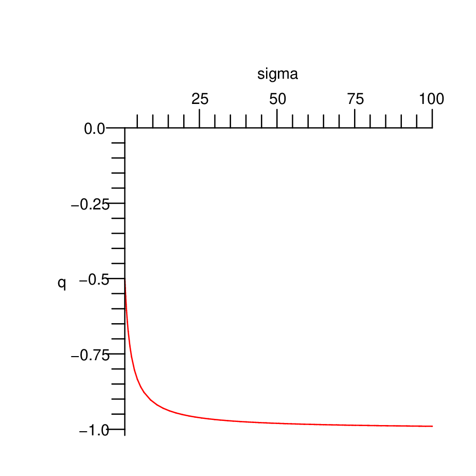
being $\sigma=\sqrt{\alpha^{2}+1}$. The behavior of $\omega_{eff}$ and $q_{eff}$ is plotted in the figures [1] and [2]. Notice that both, $\omega_{eff}$ and $q_{eff}$ remain above $-1$ for $\alpha\geq 0$ but always are negative. More specifically, for $\sigma\geq 1$ we obtain: $-0.5556\leq\omega_{eff}<-1$ and $-0.5\leq q_{eff}<-1$, which means that we are mimicking a period of quintessential expansion. On the other hand, the fact that the both parameters $\omega_{eff}$ and $q_{eff}$ remain always negative is interpreted here as the metric (1) in the present mechanism can only describe phases in the evolution of the universe which are dominated by vacuum energy, or equivalently by a cosmological parameter $\Lambda(t)$. In more general terms we can say that under the consideration of foliations like $\Sigma_{F}$ for $F=\alpha/t$ the metric in (1) is able of describing only phases of accelerated expansion of the universe.

III.3 Extracting a phantom cosmological scenario

In order to show the possibility of extract phantom cosmological scenarios by using the formalism here discussed, let us regarding the particular dynamical foliation $f(t)$ given by

$$f(t)=\beta\cosh[\bar{\alpha}(t-t_{\star})],$$ (29)

where $t_{\star}$ is the time when the period of accelerated expansion to be mimicked begins and $\beta$ and $\bar{\alpha}$ being not null constant parameters having $\beta$ units of length and $\bar{\alpha}$ units of (length) ^-1 (Note that here we are using natural units). Thus it follows from the equation (20) that the induced cosmological parameter has the form

$$\Lambda(t)=3\left[\left(\bar{\alpha}^{2}-\frac{1}{\beta^{2}}\right)\tanh^{2}[\bar{\alpha}(t-t_{\star})]+\frac{1}{\beta^{2}}\right],$$ (30)

which for values of $\beta$ and $\bar{\alpha}$ satisfying $(\bar{\alpha}\beta)^{2}<1$ is a decreasing function of time. The induced Hubble parameter according to (4) is in this case

$$H(t)=\bar{\alpha}\,\tanh[\bar{\alpha}(t-t_{\star})]+\left[\frac{1}{\beta^{2}}sech^{2}[\bar{\alpha}(t-t_{\star})]+\bar{\alpha}^{2}\tanh^{2}[\bar{\alpha}(t-t_{\star})]\right]^{1/2}.$$ (31)

Thus inserting (29) and (30) in (10) and (11) the effective EOS parameter and the deceleration parameter result respectively

$$\omega_{eff}(t) = -\frac{1}{3}\frac{2\bar{\alpha}^{2}\beta^{2}\sqrt{1+\bar{\alpha}^{2}\beta^{2}\sinh^{2}[\bar{\alpha}(t-t_{\star})]}\,\left(3\cosh^{2}[\bar{\alpha}(t-t_{\star})]-2\right)+g_{1}(t)}{g_{2}(t)\,\sqrt{1+\bar{\alpha}^{2}\beta^{2}\sinh^{2}[\bar{\alpha}(t-t_{\star})]}},$$ (32)

$$q_{eff}(t) = -\frac{\bar{\alpha}^{2}\beta^{2}\left(2\cosh^{2}[\bar{\alpha}(t-t_{\star})]-1\right)+1}{\left(\,\bar{\alpha}\beta\sinh[\bar{\alpha}(t-t_{\star})]+\sqrt{1+\bar{\alpha}^{2}\beta^{2}\sinh^{2}[\bar{\alpha}(t-t_{\star})]}\,\right)\,\sqrt{1+\bar{\alpha}^{2}\beta^{2}\sinh^{2}[\bar{\alpha}(t-t_{\star})]}},$$ (33)

being

$$g_{1}(t) = 4\bar{\alpha}\beta\sinh[\bar{\alpha}(t-t_{\star})]+6\bar{\alpha}^{3}\beta^{3}\sinh[\bar{\alpha}(t-t_{\star})]\cosh^{2}[\bar{\alpha}(t-t_{\star})]-4\bar{\alpha}^{3}\beta^{3}\sinh[\bar{\alpha}(t-t_{\star})],$$ (34)

$$g_{2}(t) = 2\bar{\alpha}^{2}\beta^{2}\cosh^{2}[\bar{\alpha}(t-t_{\star})]-2\bar{\alpha}^{2}\beta^{2}+2\bar{\alpha}\beta\sinh[\bar{\alpha}(t-t_{\star})]\sqrt{1+\bar{\alpha}^{2}\beta^{2}\sinh^{2}[\bar{\alpha}(t-t_{\star})]}+1.$$ (35)

Now in order to show that there exist suitable values of $\bar{\alpha}$ and $\beta$ leading to a phantom scenario mimicked geometrically by the use of dynamical foliations of the 5D space-time, let us to consider the values $\bar{\alpha}=1/2$ and $\beta=3/2$. With these values the temporal behavior of $\omega_{eff}$ and $q_{eff}$ is plotted in the figures [3] and [4]. In the figures we can see that we mimicked an EOS passing from a period of phantom cosmology which tends asymptotically to a de-Sitter stage.

IV Final Comments

In this letter we have derived phantom cosmologies from a 5D Riemann-flat space-time with the metric ansatz (1) and where the fifth coordinate has been regarded as noncompact. Our formalism is based on the assumption that the 5D space-time can be dynamically foliated by a family of 4D hypersurfaces $\Sigma:\psi=f(t)$. In order to induce a FRW line element on every 4D hypersurface we have adopted the continuity conditions of Ponce de Leon (3) and (4). On that framework we have shown that the energy momentum tensor geometrically induced on every dynamical hypersurface can perfectly describe a perfect fluid under the presence of a variable cosmological parameter $\Lambda(t)$. In this sense the present formalism can be considered as a way of introducing a cosmological parameter $\Lambda(t)$ geometrically from pure 5D vacuum. By reinterpreting the condition (3) we have established a geometrical criterion for assigning cosmological parameters $\Lambda(t)$ which depends only of the dynamical foliation adopted.

In the particular case when we regard the foliation $f=F^{-1}$, the induced 4D dynamics is governed by the system (5)- (6), and the induced scale factor $a(t)$ is determined by the second expression of (26). When the condition (12) is adopted it can be easily seen that this induced dynamics describes a 4D universe with an effective 4D FRW metric $ds^{2}=dt^{2}-a^{2}dr^{2}$. Under this conditions a quintessential expanding period in the evolution of the universe can be mimicked. In this case we obtain a 4D effective EOS parameter $\omega_{eff}=P_{eff}/\rho_{eff}$ and a deceleration parameter $q_{eff}$ range between $-0.5556\leq\omega_{eff}<-1$ and $-0.5\leq q_{eff}<-1$, respectively, when $\sigma\geq 1$. One interesting feature of both $\omega_{eff}$ and $q_{eff}$ is that they remain negative and always above $-1$ for $\sigma\geq 1$. This characteristic suggests that under that conditions the metric ansatz (1) can describe only periods of accelerated expansion of the universe dominated by a dark energy here mimicked by a geometrically induced cosmological parameter $\Lambda(t)$.

Finally, phantom cosmological scenarios can be also obtained by choosing a suitable dynamical foliation. More precisely we can obtain phantom scenarios from a geometrically induced cosmological parameter $\Lambda(t)$. In this case regarding for instance the particular foliation $f(t)=\beta\cosh[\bar{\alpha}(t-t_{\star})]$ we can induce for $(\bar{\alpha}\beta)^{2}<1$ a decaying cosmological parameter $\Lambda(t)$ that can lead to a phantom scenario. In particular for $\bar{\alpha}=1/2$ and $\beta=3/2$ we can achieve a phantom scenario which tends asymptotically to a de-Sitter expansion. The behavior of $\omega_{eff}$ and $q_{eff}$ for this case with respect to the parameter $\tau=t-t_{\star}$ is plotted in figures [3] and [4] respectively.

Figure 1: The figure shows the behavior of the effective EOS parameter $\omega_{eff}$ with the parameter $\sigma$.

Figure 2: The figure shows the behavior of the effective deceleration parameter $q_{eff}$ with the parameter $\sigma$.

Figure 3: The figure shows the behavior of the effective EOS parameter $\omega_{eff}$ with $\tau=t-t_{\star}$ when the values $\bar{\alpha}=1/2$ and $\beta=3/2$ are considered.

Figure 4: The figure shows the behavior of the effective deceleration parameter $q_{eff}$ with $\tau=t-t_{\star}$ when the values $\bar{\alpha}=1/2$ and $\beta=3/2$ are considered.