Phase control algorithms for focusing light through turbid media

Abstract

Light propagation in materials with microscopic inhomogeneities is affected by scattering. In scattering materials, such as powders, disordered metamaterials or biological tissue, multiple scattering on sub-wavelength particles makes light diffuse. Recently, we showed that it is possible to construct a wavefront that focuses through a solid, strongly scattering object. The focusing wavefront uniquely matches a certain configuration of the particles in the medium. To focus light through a turbid liquid or living tissue, it is necessary to dynamically adjust the wavefront as the particles in the medium move. Here we present three algorithms for constructing a wavefront that focuses through a scattering medium. We analyze the dynamic behavior of these algorithms and compare their sensitivity to measurement noise. The algorithms are compared both experimentally and using numerical simulations. The results are in good agreement with an intuitive model, which may be used to develop dynamic diffusion compensators with applications in, for example, light delivery in human tissue.

1 Introduction

Materials such as paper, white paint or human tissue are non-transparent because of multiple scattering of light [1, 2, 3]. Light propagating in such materials is diffuse. Recently, we have shown that coherent light can be focused through diffusive media yielding a sharp, intense focus [4]. Starting with the situation where a scattering object (a layer of TiO₂ pigment with a thickness of approximately 20 transport mean free paths) completely destroys the spatial coherence of the incident light (Fig. 1a, 1c), we controlled the incident wavefront to exactly match scattering in the sample. Afterwards, the transmitted light converged to a tight, high contrast focus (Fig. 1b, 1d). These matched wavefronts experience inverse diffusion, that is, they gain spatial coherence by travelling through a disordered medium.

Figure 1: Principle and experimental results of inverse wave diffusion. a) A multiply scattering object destroys the spatial coherence of incident light. b) When the same object is illuminated with a specially constructed matching wavefront, the transmitted light focuses to a tight spot. c) Recorded intensity transmission of an unshaped wave through a 10 $\mu$m thick layer of TiO₂ pigment. d) Intensity transmission through the same sample with a shaped wavefront.

For a given sample of scattering material, there is a unique incident wavefront that makes the object optimally focus light to a given point. Like a speckle pattern, this wavefront is disordered on the scale of the wavelength of light. This wavefront cannot be constructed from a small number of smooth base functions, which unfortunately renders the efficient algorithms used in adaptive optics (see e.g. [5]) ineffective. In Ref. [4], we presented an algorithm that finds the optimal wavefront when the sample is perfectly stationary and the noise level is negligible. To find applications in, for example, fluorescence excitation or photodynamic therapy, the wavefront has to be adjusted dynamically as the scatterers in the sample move. In this paper, we present two additional algorithms, that dynamically adjust the wavefront to follow changes in the sample. The performance of the algorithms is in good agreement with numerical simulations and with an analytical model. We show that the new algorithms are superior to the original algorithm when the scatterers in the sample move or when the initial signal to noise ratio is poor.

Wave diffusion is a widely encountered physical phenomenon. The use of multiple scattered waves is the subject of intensive study in the fields of, for instance, ultrasound imaging [6, 7, 8], radio and microwave antennas [9, 10], seismography [11], submarine communication [12], and surface plasmons [13]. While the algorithms discussed in this paper were developed for spatial phase shaping of light, they can be used for any type of wave and apply to spatial phase shaping as well as to frequency domain phase shaping (also known as coherent control, see e.g. [14]) as the concepts are the same.

This article is organized as follows. First the key concepts of inverse diffusion are introduced and the three different algorithms are presented. Then the experimental apparatus is explained and the measured typical performance of the algorithms is compared. In the subsequent section, we will compare the experimental results with numerical simulations and analyze the data in terms of noise and stability of the scatterers. Finally, we will analytically explain the characteristic features of the different algorithms and discuss their sensitivity to noise.

2 Algorithms for inverse diffusion

The key elements of an inverse diffusion setup are a multiply scattering sample, a spatial light modulator, an optimization algorithm and a detector, as shown in Fig. 2. The sample can be anything that scatters light without absorbing it. We will consider only samples that are thicker than approximately 6 transport mean free paths for light. Light transmitted through these samples is completely diffuse and the transmitted wavefront is completely scrambled, i.e., it has no correlation with the incident wavefront [15].

The incident wavefront is constructed using a spatial phase modulator. The modulator consists of a 2D-array of pixels that are grouped into $N$ equally sized square segments. A computer sets the phase retardation for each of the segments individually to a value between $0$ and $2\pi$. The optimization algorithm programs the phase modulator based on the detector output. Since the sample completely scrambles the incident wavefront, all segments of the wavefront are scattered independently and the optimal wavefront will not be smooth.

Behind the sample is a detector that provides feedback for the algorithm. The detector defines the target area where the intensity is maximized. The field at the detector is the result of interference from scattered light originating from the different segments of incident wavefront. When the phase of one or more segments is changed, the target intensity responds sinusoidally. We sample the sine wave by taking 10 measurements. The process of capturing a single sine wave and possibly adjusting the phase modulator accordingly is called an iteration.

The amount of control we have over the propagation of light in the disordered system is quantified by the signal enhancement. The enhancement $\eta$ is defined as

$$\eta\equiv\frac{I_{N}}{\left\langle I_{0}\right\rangle},$$ (1)

where $I_{N}$ is the intensity in the target after optimization and $\left\langle I_{0}\right\rangle$ is the ensemble averaged transmitted intensity before optimization. In a perfectly stable system, the enhancement is proportional to $N$ [4], meaning that the more individual segments are used to shape the incident wavefront, the more light is directed to the target. In practice, however, the enhancement is limited by the number of iterations that can be performed before the sample changes too much. We define the persistence time $T_{p}$ as the decay time of the field autocorrelate of the transmitted speckle, which is a measure for the temporal stability of the sample. The persistence time depends on the type of sample and on environmental conditions. Typical values of $T_{p}$ range from a few milliseconds in living tissue [16] to hours for solid samples in laboratory conditions. The other relevant timescale is the time required for performing a single iteration, $T_{i}$. In our experiments, we operate the phase modulator at just below 10 Hz and take ten measurements for each iteration; we have $T_{i}\approx 1.2$s.

Figure 2: Feedback loop for achieving inverse diffusion. An incident monochromatic beam is shaped using a spatial light modulator (1) and projected on a non-transparent multiply scattering object (2). A detector (3) detects the amount of transmitted light that reaches the target area. A feedback algorithm (4) uses the signal from the detector to program the phase modulator. Before the algorithm is started, the transmitted light forms a random speckle pattern. The algorithm changes the incident wave to increase the intensity in the target area. After a few iterations, the transmitted light focuses on the target.

We will now present three algorithms we used to invert wave diffusion. The advantages and disadvantages of the algorithms are discussed briefly and will be analyzed in detail later.

Figure 3: Principle used in the three different optimization algorithms. a) For the stepwise sequential algorithm, all segments are addressed sequentially (marked squares). After the optimal phase is measured for all segments, the modulator is updated to construct the optimal wavefront (light gray squares). b) The continuous sequential algorithm is equal to the first algorithm, except that the modulator is updated after each iteration. c) The partitioning algorithm randomly selects half of the segments and adjusts their overall phase. The modulator is updated after each measurement.

2.0.1 The stepwise sequential algorithm

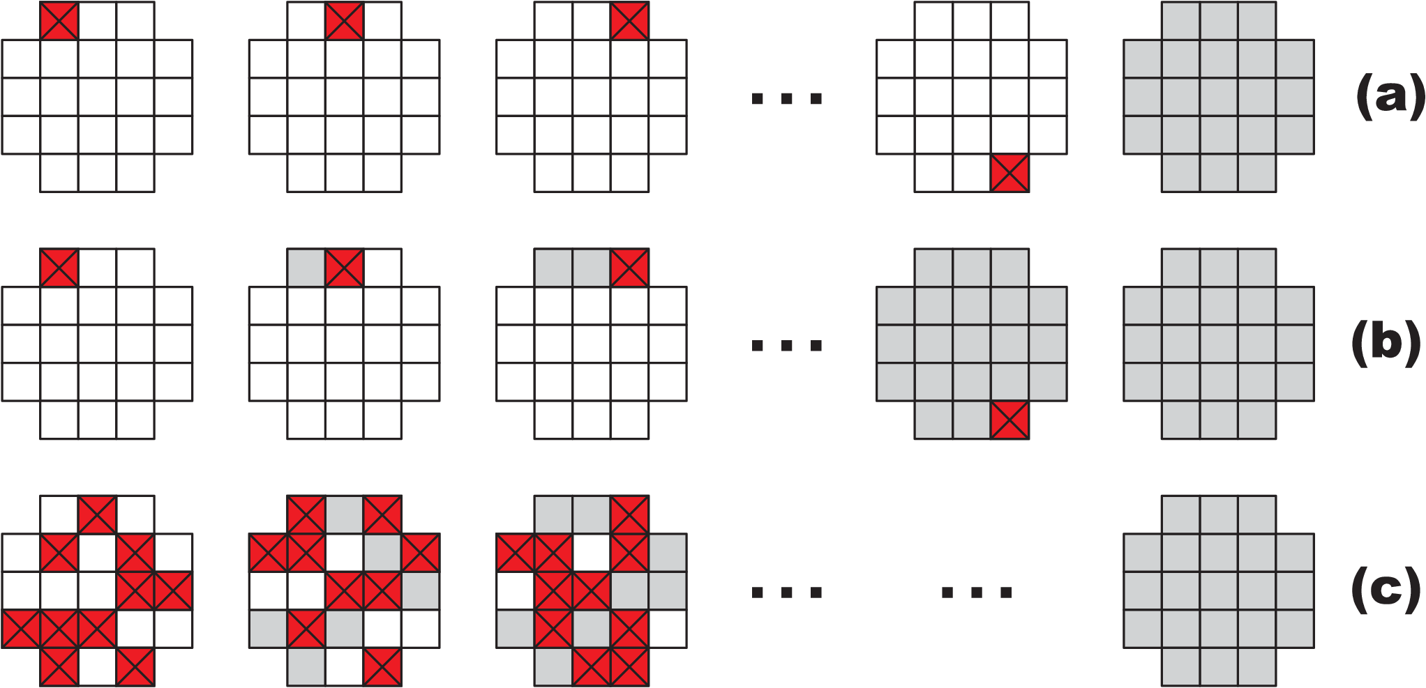
The stepwise sequential algorithm that was used in Ref. [4] is very straightforward. The computer consecutively cycles the phase of each of the $N$ segments from 0 to $2\pi$. The feedback signal is monitored and the phase for which the target intensity is maximal is stored. After all iterations are performed, the phase of each segment is set to this optimal value (see Fig. 3a). In absence of measurement noise or temporal instability, algorithm 1 is guaranteed to find the global maximum in the lowest number of iterations possible. However, when $NT_{i}\gg T_{p}$, the speckle pattern decorrelates before all measurements are performed and the algorithm will not work. Therefore, it is important to adjust the number of segments to the persistence time.

2.0.2 The continuous sequential algorithm

The continuous sequential algorithm is very similar to the stepwise sequential algorithm except for the fact that the phase of each segment is set to its maximum value directly after each measurement (see Fig. 3b). This approach has two advantages. First of all, the algorithm runs continuously and dynamically follows changes in the sample’s scattering behavior. Furthermore, the target signal starts to increase directly, which increases the signal to noise ratio of successive measurements. It is still necessary to adjust $N$ to the persistence time $T_{p}$.

2.0.3 The partitioning algorithm

As an alternative to the two sequential algorithms, we propose a partitioning algorithm that requires no a-priori information about the sample’s stability. Each iteration the phase modulator is divided randomly into two subsets, both containing half of the segments (Fig. 3c). The target intensity is maximized by changing the phase of one subset with respect to the other. Since the phase of half of the segments is changed, the initial increase in intensity will be fast and the feedback signal will be maximal. Therefore, this algorithm is expected to be less sensitive to noise and to recover from disturbances more rapidly.

3 Experiment

The different algorithms were tested experimentally using the setup shown in Fig. 4. In our case the scattering medium is a 10 $\mu$m thick layer of rutile TiO₂ pigment [17] with a mean free path of $0.55\pm 0.1$ $\mu$m, determined by measuring the total transmission at a wavelength of 632.8 nm. This sample is illuminated by a 632.8 nm HeNe laser. The laser beam is expanded and spatially modulated by a Holoeye R-2500 liquid crystal light modulator (LCD) operating in phase-mostly modulation mode [18]. The shaped beam is focused on the sample using a 63x objective with a numerical aperture (NA) of 0.85. A 20x objective (NA=0.5) images a point that is approximately $3.5$ mm behind the sample onto a 12-bit CCD camera (Allied Vision Technologies Dolphin F-145B). This point is the target area where we want the light to focus. A computer integrates the intensity in a circular area with a radius of 20 pixels (corresponding to 129 $\mu$m in the focal plane of the objective). This target area is smaller than a typical speckle spot. Using this signal as feedback, the computer programs the phase modulator using one of the algorithms described above.

Figure 4: Experimental apparatus used for inverting diffusion. Light from a HeNe laser is spatially modulated by a liquid crystal spatial light modulator (SLM). Wave plates and a polarizer are used to generate and select the polarization state for which the modulator works in phase mostly mode. The shaped beam is focused on the sample. A reference detector monitors the total intensity falling on the sample. A microscope objective, a polarizer and a CCD-camera are used to detect the intensity in the target focus, a few millimeters behind the sample.

We first run the three different algorithms with $N=52$. Since $T_{p}/T_{i}\gg 52$, we do not expect to see decoherence effects. In total, 208 iterations were performed, which means that the sequential algorithms ran four times consecutively. The results of the optimization procedures is shown in Fig. 5a. Although the three algorithms reach the same final enhancement of intensity, there are significant differences between the algorithms. The enhancement for the stepwise sequential algorithm increases in discrete steps because the phase modulator is only reprogrammed every $N$ iterations. During the first $N$ iterations, the target signal is low and the algorithm suffers from noise. The saturation enhancement is reached after the second update (after $2N$ iterations). The continuous sequential algorithm and the partitioning algorithm both start updating the wavefront immediately and, therefore, have a higher initial increase of the signal. The continuous sequential algorithm is the first algorithm to reach the saturation enhancement (after $N$ iterations). The partitioning algorithm has the fastest initial increase in the target signal. It is, however, the last algorithm to reach the saturation enhancement since the final convergence is very slow.

Figure 5: (a) Typical runs of the stepwise sequential algorithm (dotted line), the continuous sequential algorithm (dashed line) and the partitioning algorithm (solid line). All algorithms were run with $N=52$. The sequential algorithms were repeated four times. (b) Simulation results for $N=52$ averaged over 64 runs. The simulation captures the main features of the three algorithms, but predicts a higher maximum enhancement.

When the number of segments in the wavefront is increased, we expect to find a higher target intensity. Figure 6a shows the experimental results for $N=1804$ on a logarithmic scale. The final intensity enhancement is approximately 40 times higher than in Fig. 5a. A further difference is that in this situation the effects of decoherence are no longer negligible. This effect is most clearly visible with the stepwise sequential algorithm. The phase modulator is updated after each $N$ iterations and between the updates the intensity decays exponentially with a $1/e$ decay of about $T_{p}/T_{i}=5000$ iterations.

The convergence behavior of the three algorithms is similar to the experiment shown in Fig. 5. The partitioning algorithm clearly causes a higher signal enhancement during the first 1000 iterations. The initial increase in the enhancement is linear with a slope of 0.37. Initially, this linear increase is far superior to the quadratic increase obtained with the continuous sequential algorithm.

We conclude that both new algorithms are valuable improvements over the original stepwise sequential algorithm. These algorithms are far less sensitive to noise and the target signal is kept at a constant value even in the presence of decoherence. The partitioning algorithm has the fastest initial increase and therefore will recover from disturbances most rapidly.

Figure 6: (a) Typical runs of stepwise sequential algorithm (dotted line), the continuous sequential algorithm (dashed line) and the partitioning algorithm (solid line). All algorithms were run with $N=1804$. The enhancement are plotted on a logarithmic scale. (b) Simulation results for $N=1804$ averaged over 64 runs.

4 Simulations

In order to obtain a better understanding of the effects of noise and fluctuations on the performance of the different algorithms we perform numerical simulations. The disordered medium is represented by a transmission matrix with elements drawn from a circular Gaussian distribution (more details on the matrix representation can be found below). Decoherence is modelled by adding a small perturbation to the transmission matrix after every measurement. Finally, measurement noise is included by adding a random value to the simulated detector signal.

Figures 5b and 6b show the simulated enhancement for a system with $T_{p}/T_{i}=5000$. Every iteration, ten measurements are performed for phase delays between $0$ and $2\pi$. To each of these measurements, Gaussian noise with a standard deviation of $0.3I_{0}$ was added. The magnitude of the noise is comparable to experimental observations. The three different algorithms were run with $N=52$ and $N=1804$ to simulate the experiments shown in Fig. 5a and Fig. 6a.

The simulations are in good qualitative agreement with the experimental data. The result for the stepwise sequential algorithm shows that the effects of noise and decoherence are simulated realistically. Furthermore, the initial signal increase and the long time convergence behavior correspond to the measured results. The only significant difference is the 20% to 50% higher enhancement reached in the simulations. A possible explanation for this difference is the residual amplitude cross-modulation in our phase modulator. Due to this cross-modulation, the optimal wavefront cannot be generated exactly. Furthermore, the amplitude modulation decreases the accuracy of the measurement of the optimal phase. The partitioning algorithm is less sensitive to this last effect since the cross-modulation is averaged over many segments with different phases. Since the simulations capture the overall behavior of the algorithms very well, we can use them to extrapolate to situations with a lot of noise and strong decoherence or, on the other hand, to perfectly stable systems.

5 Analytical expressions for the enhancement

In this section, we analyze the performance of the algorithms with analytical theory and compare these results to the simulations. We describe scattering in the sample with the transmission matrix elements, $t_{mn}$. This matrix couples the fields of the incident light and the transmitted light.

$$E_{m}=\sum_{n}^{N}t_{mn}A_{n}e^{i\phi_{n}},$$ (2)

where the $\phi_{n}$ is the phase of the $n$th segment of the phase modulator. Assuming that the modulator is illuminated homogeneously, all incoming channels carry the same intensity. We write $A_{n}=1/\sqrt{N}$ to normalize the total incident intensity. Elements $E_{1},E_{2},\ldots$ correspond to single scattering channels of the transmitted light. Since we are interested in focusing light to a single spot, we need to consider only a single transmission channel, $E_{m}$. The intensity transmitted into channel $m$ is given by

$$|E_{m}|^{2}=\frac{1}{N}\left|\sum_{n}^{N}t_{mn}e^{i\phi_{n}}\right|^{2}.$$ (3)

Regardless of the values of the elements $t_{mn}$ of the transmission matrix, the intensity $|E_{m}|^{2}$ has its global maximum when the phase modulator exactly compensates the phase retardation in the sample for each segment, i.e. $\phi_{n}=-\arg(t_{mn})$. The target intensities before optimization ($I_{0}$) and after an ideal optimization ($I_{\text{max}}$) are given by

$$I_{0}=\frac{1}{N}\left|\sum_{n}^{N}t_{mn}\right|^{2},$$ (4)

and

$$I_{\text{max}}=\frac{1}{N}\left(\sum_{n}^{N}\left|t_{mn}\right|\right)^{2}.$$ (5)

For a disordered medium the elements of $t_{mn}$ are independent and have a Gaussian distribution [19, 20, 21, 22]. Rewriting Eq. (5) gives

$$\left\langle I_{\text{max}}\right\rangle =\left\langle\frac{1}{N}\sum^{N}_{n,k\neq n}|t_{mn}||t_{mk}|+\frac{1}{N}\sum_{n}^{N}|t_{mn}|^{2}\right\rangle,$$ (6)

$$=\left\langle I_{0}\right\rangle\left[(N-1)\frac{\pi}{4}+1\right],$$ (7)

where the angled brackets denote ensemble averaging over disorder. Eq. (7) predicts that the expected maximum enhancement for an ideally stable, noise free system linearly depends on the number of segments $N$. For $N\gg 1$, we have $\eta\approx\pi N/4$.

5.1 Performance in fluctuating environments

In reality, the sample will not be completely stable. Whether this instability is due to a drift of the sample position, movement of the scatterers, changing humidity or any other cause, the transmission matrix will fluctuate over time. In the simulations, we modelled decoherence by repeatedly adding a small perturbation to each of the matrix elements.

$$t_{mn}\rightarrow\frac{1}{\sqrt{1+\delta^{2}}}(t_{mn}+\xi),$$ (8)

where $\xi$ is drawn from a complex Gaussian distribution with mean 0 and standard deviation $\delta$. The prefactor normalizes the transformation so that $\left\langle|t|^{2}\right\rangle$ remains constant. By substituting the continuous limit of Eq. (8) in Eq. (6), we find an analytic expression for the effect of decoherence,

$$\left\langle I_{N}\right\rangle=\left\langle I_{0}\right\rangle\left[\frac{\pi}{4N}\left(\sum^{N}_{n}e^{-T_{n}\delta^{2}/(2T_{i})}\right)^{2}+O(1)\right],$$ (9)

where $T_{n}$ is the time that has past since the phase of segment $n$ was measured. This simple model explains the exponential decay of the intensity that was observed in the measurements (see Fig.6a) and predicts a decay time of $T_{p}=T_{i}/\delta^{2}$.

We now calculate the maximum enhancement that can be reached with the continuous sequential algorithm in the presence of decoherence. Because the phases of the segments are measured sequentially, at any given time the values for $T_{n}$ are equally spaced between $1$ and $N$. From Eq. (9) we find a maximum intensity enhancement of

$$\eta_{N}\equiv\frac{\left\langle I_{N}\right\rangle}{\left\langle I_{0}\right\rangle}=\frac{\pi}{4N}\left(\frac{1-e^{-NT_{i}/(2T_{p})}}{e^{T_{i}/(2T_{p})}-1}\right)^{2}+O(1).$$ (10)

The maximum enhancement for both sequential algorithms is the same. However, since the stepwise algorithm only updates the projected wavefront after $N$ iterations, the enhancement decreases exponentially between updates.

Figure 7: Theoretical maximum enhancement as a function of coherence time for different algorithms. The solid lines represent the maximum enhancement that can be obtained using the sequential algorithms. The enhancement depends on the number of segments used in the algorithm. The dashed line shows the enhancement for the partitioning algorithm where $N\gg T_{p}/T_{i}$.

In Fig. 7 the enhancement for different values of $N$ is plotted versus $T_{p}/T_{i}$. When the persistence time is large ($T_{p}/T_{i}\gg N$), decoherence effects do not play a role and the enhancement linearly depends on $N$ as was seen in Eq. (7). For $T_{p}/T_{i}<N$, however, the enhancement decreases because the speckle pattern decorrelates before all iterations are performed and the enhancement drops to zero. As a consequence, the sequential algorithms only perform optimal when $N$ is adjusted to $T_{p}$. When $T_{p}$ is known a-priori, this optimum for $N$ can be found by maximizing Eq. (10). We find

$$N_{\text{opt}}=WT_{p}/T_{i},$$ (11)

where $W\approx 2.51$ is the solution of $\exp(W/2)=1+W$. The maximal enhancement achievable with sequential algorithms follows by substituting Eq. (11) into Eq. (10) and equals $\eta_{\text{opt}}=0.640T_{p}/T_{i}$.

With the partitioning algorithm $\eta$ increases by $1/2$ each iteration of the algorithm (see appendix A). As long as $N\gg T_{p}/T_{i}$, the enhancement saturates at $\eta=T_{p}/(2T_{i})+1$, when the increase is exactly cancelled by the effect of decoherence. The most important difference with the sequential algorithms, is that the enhancement reached with the partitioning algorithm does not depend on $N$. In Fig. 7 it can be seen that the partitioning algorithm outperforms the sequential algorithms for almost all combinations of $T_{p}$ and $N$. The sequential algorithm only give a slightly higher enhancement when they are fine-tuned for a known persistence time ($N=2.51T_{p}/T_{i}$). In most situations, $T_{p}$ is not known a-priory or varies over time and the partitioning algorithm will be preferable.

Our analytical results for all three algorithms are supported by numerical simulations (see Fig. 8). The simulations exactly reproduce the theoretical curves shown in Fig. 7. For the simulations we used $N=4096$, a number that can easily be reached with a LCD phase modulator. Again, the partitioning algorithm can be seen to have good overall performance, whereas the sequential algorithms only work well for certain combinations of $N$ and $T_{p}$.

In conclusion, the maximum enhancement that can be reached linearly depends on the sample’s persistence time. For the sequential algorithms $\eta=0.64T_{p}/T_{i}$, but only when $N$ is precisely adjusted to $T_{p}$. The partitioning algorithm has $\eta=0.5T_{p}/T_{i}$, as long as $N$ is large enough. Using these analytical relations, the performance of each of the three algorithms in different experimental situations can easily be estimated.

Figure 8: Simulated effect of decoherence on the sequential algorithms (solid line) and on the partitioning algorithm (dashed line). The simulations are averaged over 25 runs. Only when $N\approx 2.51T_{p}/T_{i}$, the sequential algorithms perform slightly better than the partitioning algorithm.

6 Effect of Noise

	stepwise	continuous	partitioning
	sequential	sequential
signal	$2I_{0}\sqrt{1/N}$	$2I_{0}\sqrt{\eta/N}$	$\eta I_{0}$
bias	$I_{0}$	$\eta I_{0}$	$\eta I_{0}$
relative shot noise SNR	$2\sqrt{I_{0}/N}$	2$\sqrt{I_{0}/N}$	$\sqrt{\eta I_{0}}$
rms phase correction	$\sqrt{3}\pi$	$\sqrt{3}\pi$	$\sqrt{2/\eta}$

Table 1: Signal and noise characteristics of the three algorithms. The rms phase correction is a measure for the required sensitivity.

Measurement noise affects the measured phases. Noise induced errors in the phases lead to a reduction of the enhancement, $\eta$. We will now compare the signal-to-noise ratio (SNR) of the three different algorithms. In a single iteration of an algorithm, the phase of one or more segments is varied, while the phase of the other segments is kept constant. The intensity at the detector equals

$$I(\Phi)=I_{A}+I_{B}+2\sqrt{I_{A}I_{B}}\cos{(\Phi-\Phi_{0})},$$ (12)

where $I_{B}$ is the intensity at the target originating from the modulated segments, $I_{A}$ is the target intensity caused by light coming from the other segments, $\Phi$ is the phase that is varied and $\Phi_{0}$ is the unknown optimal value for the phase. The last term in Eq. (12) is the signal that is relevant for measuring $\Phi_{0}$. There first two terms constitute a constant bias.

Table 1 lists the magnitudes of the signal and the bias for each of the three algorithms. If the detection system is photon shot noise limited, the noise is proportional to the square root of the bias. When, on the other hand, constant noise sources such as readout noise or thermal noise are dominant, the SNR is directly proportional to the signal magnitude. Table 1 also shows the root mean square (rms) phase correction that is applied during each iteration of the corresponding algorithm. The rms phase correction is a measure for the required accuracy of the measurements.

With the stepwise sequential algorithm, $I_{A}\approx I_{0}$ and on average $I_{B}=I_{0}/N$. Since the initial diffuse transmission $I_{0}$ is low and $N$ can be very high, the SNR is low. The continuous sequential algorithm has a higher SNR since the overall intensity at the detector increases while the algorithm progresses and $I_{A}\approx\eta I_{0}$. Assuming the dominant noise source is constant, the SNR will increase as the enhancement becomes higher. Therefore, the algorithm can be accelerated by decreasing the integration time of the camera as the algorithm advances. In case the detection system is photon shot noise limited, the SNR remains constant during the optimization since both the signal and the shot noise scale as $\sqrt{\eta I_{0}}$.

The highest SNR is achieved with the partitioning algorithm. Since we always change the phase of half of the segments, $I_{A}\approx I_{B}\approx\eta I_{0}/2$, resulting in a maximal signal. Unlike the sequential algorithms, the SNR does not depend on $N$. Therefore the number of segments can be increased without suffering from noise. Like with the continuous sequential algorithm, the integration time can be adjusted dynamically to optimize the speed/SNR tradeoff. Although the partitioning algorithm has the highest SNR, the magnitude of the phase corrections decreases as the algorithm progresses. The required accuracy in measuring $\Phi_{0}$ increases at the same pace as the SNR increases.

The partitioning algorithm is very sensitive to measurement errors since, when the measured $\Phi_{0}$ has an error, half of the segments will be programmed with the wrong phase. In the extreme case where the error equals $\pi$ the enhancement completely disappears in a single iteration. A simple and effective solution to this problem is to keep the previous configuration of the phase modulator in memory. When an optimization step causes the signal to decrease, the algorithm can revert to the saved configuration.

7 Conclusion

Three different algorithms for inverting wave diffusion were presented. The algorithms were compared experimentally, with numerical simulations and using analytical theory. We found good agreement between experimental data, simulations and theory. Moreover, the simulations and theory can be used to predict the performance in different experimental situations.

The effectiveness of the algorithms was quantified by the enhancement. It was seen that the enhancement depends on the number of segments $N$ and the relative persistence time $T_{p}/T_{i}$. For the sequential algorithms to have optimal performance, it is required to adjust $N$ to match $T_{p}$. This means that these algorithms need a-priori knowledge of the system. The partitioning algorithm does not need this knowledge and always performs close to optimal. Moreover, the algorithm causes the enhancement to increase the most rapidly of the three investigated methods. All in all, this algorithm is a good candidate for applying inverse diffusion in instable scattering media such as living tissue. In the future, learning algorithms (see e.g. [23, 24]) might be developed to further improve the performance of inverse diffusion, for instance by dynamically balancing the trade-off between signal to noise ratio and measurement speed.

The maximum enhancement linearly depends on the number of measurements that can be performed before the speckle pattern decorrelates ($T_{p}/T_{i}$). The faster the measurements, the higher the enhancement. In our current system, the speed is limited by the response time of the LCD. Fast micro mechanical phase modulators have a mechanical response time of about 10 $\mu$s (see e.g. [25]), which allows a $10^{4}$ times faster operation than with our current system. In perfused tissue, a typical decorrelation timescale is 10 ms [16], which means that an enhancement of about 50 should be possible with currently available technology.

8 Acknowledgements

We thank Prof. Ad Lagendijk and Prof. Willem Vos for support and valuable discussions. This work is part of the research program of the “Stichting voor Fundamenteel Onderzoek der Materie (FOM)”, which is financially supported by the “Nederlandse Organisatie voor Wetenschappelijk Onderzoek (NWO)”.

Appendix A Calculation of the performance of the partitioning algorithm

In this appendix we calculate the development of the enhancement of the partitioning algorithm under ideal conditions. During one iteration of the partitioning algorithm, the phase modulator is randomly split into two groups ($A$ and $B$), each containing half of the segments. The relative phase ($\Phi$) of group $B$ is cycled from 0 to $2\pi$. During this cycle, the target intensity is given by

$$I(\Phi)=\left|E_{mA}+E_{mB}e^{i\Phi}\right|^{2},$$ (13)

where $E_{mA}$ is the contribution of the segments in group $A$ to the target field

$$E_{mA}=\sum_{n\in A}\sqrt{\frac{\left\langle I_{0}\right\rangle}{N}}\xi_{mn},$$ (14)

with

$$\xi_{mn}\equiv\sqrt{\frac{1}{\left\langle I_{0}\right\rangle}}t_{mn}e^{i\phi_{n}},$$ (15)

and similar for $E_{mB}$. The coefficients $\xi_{mn}$ are initially random and distributed according to a normalized circular Gaussian distribution, meaning that $\left\langle\xi\right\rangle=0$ and $\left\langle(\text{Re}\;{\xi})^{2}\right\rangle=\left\langle(\text{Im}\;{\xi})^{2}\right\rangle=1/2$. As the algorithm proceeds, the phases $\phi_{n}$ are adjusted and the distribution gradually changes to a Rayleigh distribution when a high enhancement is reached. The average value $\left\langle\xi\right\rangle$ increases from $0$ to $\sqrt{\pi/4}$ as all contributions are aligned to be in phase. At any moment during the optimization, $\left\langle\xi\right\rangle=\sqrt{(\eta-1)/(N-1)}$ and $\left\langle|\xi|^{2}\right\rangle=1$.

Figure 9 gives a graphical representation of a single iteration. Before the iteration, $E_{mA}$ and $E_{mB}$ have a different phase. Without loss of generality, we choose the phase of $(E_{mA}+E_{mB})$ to be $0$. The intensity before the iteration is given by

$$I_{\text{before}}=\left(\text{Re}\;E_{mA}+\text{Re}\;E_{mB}\right)^{2}.$$ (16)

After the iteration, $\Phi$ is set to the value that caused the highest target intensity, which means that $E_{mA}$ and $E_{mB}$ are now in phase. The target intensity then equals

$$I_{\text{after}}=\left(|E_{mA}|+|E_{mB}|\right)^{2},$$ (17)

which is higher than or equal to before the iteration.

Figure 9: Complex plane representation of the partitioning algorithm. a) Before the iteration the contributions from $A$ and $B$ are not exactly in phase. b) After the iteration, the contributions are aligned and the resulting intensity is higher.

We now calculate the average intensity gained in a single iteration. We consider the regime where already a few iterations have been done ($\eta\gg 1$). In this regime, we can approximate

$$|E_{mA}| =\sqrt{(\text{Re}\;E_{mA})^{2}+(\text{Im}\;E_{mA})^{2}}$$ (18)

$$\approx\text{Re}\;E_{mA}+\frac{(\text{Im}\;E_{mA})^{2}}{2\text{Re}\;E_{mA}}.$$ (19)

Using this result in Eq. (17) gives

$$I_{\text{after}}=\left(\text{Re}\;E_{mA}+\text{Re}\;E_{mB}|\right)^{2}+(\text{Im}\;E_{mA})^{2}+(\text{Im}\;E_{mB})^{2}+\\ +\frac{\text{Re}\;{E_{mA}}}{\text{Re}\;{E_{mB}}}(\text{Im}\;E_{mB})^{2}+\frac{\text{Re}\;{E_{mB}}}{\text{Re}\;{E_{mA}}}(\text{Im}\;E_{mA})^{2}+\\ +\frac{(\text{Im}\;E_{mA})^{4}}{4(\text{Re}\;E_{mA})^{2}}+\frac{(\text{Im}\;E_{mB})^{4}}{4(\text{Re}\;E_{mB})^{2}}+\frac{(\text{Im}\;E_{mA}\text{Im}\;E_{mB})^{2}}{2\text{Re}\;E_{mA}\text{Re}\;E_{mB}}$$ (20)

where the terms on the last line can be neglected. If $N\gg 1$,
$\text{Re}\;{E_{mB}}/\text{Re}\;{E_{mA}}\approx 1$. The intensity gain for the iteration $\Delta I\equiv I_{\text{after}}-I_{\text{before}}$ is now found to be

$$\Delta I=2(\text{Im}\;E_{mA})^{2}+2(\text{Im}\;E_{mB})^{2}$$ (21)

We are primarily interested in the regime $N\gg\eta\gg 1$), where the algorithm picks up the main part of the final enhancement. In this regime, $\left\langle\xi\right\rangle\ll 1$ and the probability distribution of $\xi$ is still close to the original Gaussian distribution. Therefore, $\left\langle(\text{Im}\;{\xi})^{2}\right\rangle\approx 1/2$ and it follows from Eq. (14) that

$$\Delta I=\frac{1}{2}\left\langle I_{0}\right\rangle$$ (22)

Therefore, we expect the intensity enhancement $\eta$ to increase with $1/2$ after each iteration of the algorithm. With this information, we also calculate the typical phase adjustment that is performed in each iteration. From Fig. 9 it follows that the root mean square phase adjustment equals

$$\Phi_{\text{rms}}\equiv\sqrt{\left\langle\Phi\right\rangle}=\sqrt{\left\langle\frac{(\text{Im}\;E_{mA})^{2}}{(\text{Re}\;E_{mA})^{2}}\right\rangle}=\sqrt{\frac{2}{\eta}}$$ (23)

When $\eta$ approaches its maximum, all contributions are almost completely in phase and $\left\langle(\text{Im}\;{\xi})^{2}\right\rangle$ vanishes. In this regime, the algorithm becomes less and less effective, as was seen in simulations and experiments (see Fig. 6).

References

- [1] E. A. Milne, Radiative equilibrium in the outer layers of a star, Monthly Not. Roy. Astron. Soc. 81 (1921) 361–375.
- [2] S. Chandrasekhar, Radiative Transfer, Dover Publications, Inc., New York, 1960.
- [3] A. Ishimaru, Limitation on image resolution imposed by a random medium, Appl. Opt. 17 (1978) 348–352.
- [4] I. M. Vellekoop, A. P. Mosk, Focusing coherent light through opaque strongly scattering media, Optics Lett. 32 (16) (2007) 2309–2311.
- [5] R. K. Tyson, Principles of Adaptive Optics, 2nd Edition, Academic Press, 1998.
- [6] M. Fink, D. Cassereau, A. Derode, C. Prada, P. Roux, M. Tanter, J.-L. Thomas, F. Wu, Time-reversed acoustics, Rep. Prog. Phys. 63 (1999) 1933–1995.
- [7] O. I. Lobkis, R. L. Weaver, On the emergence of the green’s function in the correlations of a diffuse field, J. Ac. Soc. Am. 110 (6) (2001) 3011–3017.
- [8] L. Borcea, G. Papanicolaou, C. Tsogka, Interferometric array imaging in clutter, Inv. Prob. 21 (2005) 1419–1460.
- [9] G. Lerosey, J. de Rosny, A. Tourin, M. Fink, Focusing beyond the diffraction limit with far-field time reversal, Science 315 (2007) 1120–1122.
- [10] G. J. Foschini, Layered space-time architecture for wireless communication in a fading environment when using multi-element antennas, Bell Labs Technical Journal 1 (1996) 41–59.
- [11] N. M. Shapiro, M. Campillo, L. Stehly, M. H. Ritzwoller, High-resolution surface-wave tomography from ambient seismic noise, Science 307 (2005) 1615.
- [12] W. A. Kuperman, W. S. Hodgkiss, H. C. Song, T. Akal, C. Ferla, D. R. Jackson, Phase conjugation in the ocean: Experimental demonstration of an acoustic time-reversal mirror, J. Acoust. Soc. Am. 103 (1998) 25–40.
- [13] M. I. Stockman, S. V. Faleev, D. J. Bergman, Coherent control of femtosecond energy localization in nanosystems, Phys. Rev. Lett. 88 (6) (2002) 067402.
- [14] J. L. Herek, W. Wohlleben, R. J. Cogdell, D. Zeidler, M. Motzkus, Quantum control of energy flow in light harvesting., Nature 417 (2002) 533–535.
- [15] R. Pappu, B. Recht, J. Taylor, N. Gershenfeld, Physical one-way functions, Science 297 (2002) 2026–2030.
- [16] J. D. Briers, S. Webster, Quasi real-time digital version of single-exposure speckle photography for full-field monitoring of velocity or flow fields, Opt. Commun. 116 (1) (1995) 36–42.
- [17] R. H. J. Kop, P. de Vries, R. Sprik, A. Lagendijk, Observation of anomalous transport of strongly multiple scattered light in thin disordered slabs, Phys. Rev. Lett. 79 (22) (1997) 4369–4372.
- [18] J. A. Davis, J. Nicolás, A. Márquez, Phasor analysis of eigenvectors generated in liquid-crystal displays, Appl. Opt. 41 (22) (2002) 4579–4584.
- [19] J. W. Goodman, Statistical optics, Wiley, New York, 2000.
- [20] N. Garcia, A. Z. Genack, Crossover to strong intensity correlation for microwave radiation in random media, Phys. Rev. Lett. 63 (1989) 1678–1681.
- [21] M. A. Webster, T. D. Gerke, A. M. Weiner, K. J. Webb, Spectral and temporal speckle field measurements of a random medium, Opt. Lett. 29 (13) (2004) 1491.
- [22] C. W. J. Beenakker, Random-matrix theory of quantum transport, Rev. Mod. Phys. 69 (1997) 731–808.
- [23] D. E. Goldberg, Genetic algorithms in search, optimization & machine learning, Addison-Wesley, Reading, MA, 1989.
- [24] R. S. Judson, H. Rabitz, Teaching lasers to control molecules, Phys. Rev. Lett. 68 (1992) 1500–1503.
- [25] M. Hacker, G. Stobrawa, R. Sauerbrey, T. Buckup, M. Motzkus, M. Wildenhain, A. Gehner, Micromirror slm for femtosecond pulse shaping in the ultraviolet, Appl. Phys. B 76 (2003) 711.