NNLO fermionic corrections to the charm quark mass dependent matrix elements in $\bar{B}\to X_{s}\gamma$

Abstract: 

We compute the virtual ${\mathcal{O}}\left(\alpha_{s}^{2}\right)$ fermionic contributions to the charm quark mass dependent matrix elements of the $\bar{B}\to X_{s}\gamma$ decay. In the case of a massless quark loop insertion into the gluon propagator, our result obtained as an expansion in $z=m_{c}^{2}/m_{b}^{2}$ and an exact expression in terms of multi-fold MB integrals, confirms the findings of Bieri, Greub and Steinhauser  [20]. We observe, however, large deviations in the case of a b-quark loop insertion. The charm quark loop shows smaller, but still noticeable differences.

1 Introduction

One of the most interesting rare B-meson decays is the inclusive $\bar{B}\,\to X_{s}\gamma$ mode which provides precise and clean short-distance information on $\Delta B\,=\,1$ flavor changing neutral currents (FCNCs). This process occurs in the SM only at the loop level, through the exchange of W-bosons and up-type quarks, making it highly sensitive to non-standard effects which are not suppressed by additional factors $\alpha$ relative to the SM contributions. Combined with the low sensitivity of $B\to X_{s}\gamma$ to non-perturbative effects, this makes it possible to observe new physics contributions indirectly, or to set limits on the relevant masses and coupling parameters. In fact the decay width $\Gamma\left(\bar{B}\to X_{s}\gamma\right)$ is well approximated by the partonic decay rate $\Gamma(b\to X_{s}^{parton}\gamma)$ which can be analyzed within the framework of renormalization-group-improved perturbation theory .

In view of the above, it is obvious that both accurate measurements and precise theoretical SM calculations, with a good control of both perturbative and non-perturbative corrections, have to be provided. As far as the experimental side is concerned, measurements are performed by several B physics experiments operating within various experimental settings: CLEO [1] (Cornell), BaBaR [2] (SLAC), Belle [3] (KEK) and ALEPH [4] (CERN) . Combining the measurements of the first three (the last one has very large error bars) for the branching ratio ${\mathcal{B}}(\bar{B}\to X_{s}\gamma)$ leads to a world average with a cut $E_{\gamma}>1.6\;$GeV in the ${\bar{B}}$-meson rest frame which reads [5]

$${\mathcal{B}}(\bar{B}\to X_{s}\gamma)_{\scriptscriptstyle E_{\gamma}>1.6\,{\rm GeV}}^{\scriptscriptstyle\rm exp}=\left(3.55\pm 0.24{\;}^{+0.09}_{-0.10}\pm 0.03\right)\times 10^{-4},$$ (1)

where the first error is given by the statistic and systematic uncertainty, the second one is due to the theory input on the shape function, and the third one is caused by the $b\to d\gamma$ contamination . This average is in good agreement with the recent theoretical estimate including known next-to-next-to-leading-order (NNLO) effects  [6]

$${\mathcal{B}}({\bar{B}}\to X_{s}\gamma)_{\scriptscriptstyle E_{\gamma}>1.6\,{\rm GeV}}^{\scriptscriptstyle\rm theo}=(3.15\pm 0.23)\times 10^{-4},$$ (2)

where the error consists of four types of uncertainties added in quadrature: non-perturbative (5%), parametric (3%), higher-order (3%) and $m_{c}$-interpolation ambiguity (3%).

The total experimental error of about 7% in Eq. (1) is of the same size as the expected ${\mathcal{O}}(\alpha_{s}^{2})$ corrections to the perturbative transition $b\to X_{s}^{\rm parton}\gamma$ [7], which calls for completing the SM calculations with this accuracy level.

QCD corrections to the partonic decay rate $\Gamma\left(b\to s\gamma\right)$ contain large logarithms of the form $\alpha_{s}^{n}\left(m_{b}\right)\,\ln^{m}\left(m_{b}/M\right)$, where $M\,=\,m_{t}$ or $M\,=\,m_{W}$ and $m\leq n$ (with $n\,~=~\,0,1,2,\dots$) . In order to get a reasonable prediction for the decay rate with next-to-next-leading-log (NNLL) precision, it is necessary to resum logarithms with ($m\,=\,n\,,n-1,\,n-2$) with the help of renormalization-group techniques. A convenient framework is an effective low-energy theory obtained from the SM by decoupling the heavy electroweak bosons and the top quark . The resulting effective Lagrangian, given in the next section, is a product of the Wilson coefficients $C_{i}(\mu)$ which play the role of coupling constants, and local flavor-changing operators $Q_{i}(\mu)$ .

As far as the next-to-leading order corrections are concerned, the program has been completed already a few years ago, thanks to the joint effort of many groups (see e.g. [8, 9] and references therein). Moreover, each of the ingredients has been cross-checked by more than one group. The next-to-next-to-leading order calculation, which involves hundreds of three-loop on-shell vertex-diagrams and thousands of four-loop tadpole-diagrams, is a very complicated task and is currently under way . A consistent calculation of $b\to s\gamma$ at this order requires three steps:

• Matching:  Evaluation of $C_{i}(\mu_{0})$ at the renormalization scale $\mu_{0}\sim M_{W},m_{t}$  by requiring equality of the SM and effective theory Green’s functions at the leading order in (external momenta)$/(M_{W},m_{t})$ to ${\mathcal{O}}\left(\alpha_{s}^{2}\right)$ . All the relevant Wilson coefficients have already been calculated [11, 12] to this precision, by matching the four-quark operators $Q_{1},\dots,Q_{6}$ and the dipole operators $Q_{7}$ and $Q_{8}$ at the two- and three-loop level respectively.

• Mixing:  Calculation of the operator mixing under renormalization, by deriving the effective theory Renormalization Group Equations (RGE) and evolving $C_{i}(\mu)$ from $\mu_{0}$ down to the low-energy scale $\mu_{b}\sim m_{b}$, using the anomalous-dimension matrix (ADM) to ${\mathcal{O}}\left(\alpha_{s}^{3}\right)$ . Here, the three-loop renormalization in the $\{Q_{1},\dots,Q_{6}\}$ and $\{Q_{7},Q_{8}\}$ sectors was found in [13, 14], and results for the four-loop mixing of $Q_{1},\dots,Q_{6}$ into $Q_{7}$ and $Q_{8}$ were recently provided in [15], thus completing the anomalous-dimension matrix.

• Matrix elements:  Evaluation of the on-shell $b\to s\gamma$ amplitudes at  $\mu_{b}~\sim~m_{b}$  to ${\mathcal{O}}\left(\alpha_{s}^{2}\right)$. This task is not complete yet, although a number of contributions is known. The two-loop matrix element of the photonic dipole operator $Q_{7}$, together with the corresponding bremsstrahlung, was found in [16, 17], confirmed in [18] and subsequently extended to include the full charm quark mass dependence in [19]. In [20], the ${\mathcal{O}}\left(\alpha_{s}^{2}\,n_{f}\right)$ contributions were found to the two-loop matrix elements of $Q_{7}$ and $Q_{8}$, as well as to the three-loop matrix elements of $Q_{1}$ and $Q_{2}$, using an expansion in the quark mass ratio $m_{c}^{2}/m_{b}^{2}$. Diagrammatically, these parts are generated by inserting a one-loop quark bubble into the gluon propagator of the two-loop Feynman diagrams. Naive non-abelianization (NNA) is then used to get an estimate of the complete corrections of ${\mathcal{O}}\left(\alpha_{s}^{2}\right)$ by replacing $n_{f}$ with $-\frac{3}{2}\beta_{0}$. Moreover, the contributions of the dominant operators at ${\mathcal{O}}\left(\alpha_{s}^{2}\beta_{0}\right)$ to the photon energy spectrum have been computed in [21]. Finally, in [22], the full matrix elements of $Q_{1}$ and $Q_{2}$ have been computed in the large $m_{c}$ limit, $m_{c}\gg m_{b}/2$. Subsequently, an interpolation in the charm quark mass has been done down to the physical region, under the assumption that the $\beta_{0}$-part is a good approximation at $m_{c}\,=\,0$ . This is the source of the interpolation uncertainty that has been mentioned below Eq. (2).

To date, no independent check has been provided for the ${\mathcal{O}}\left(\alpha_{s}^{2}\,n_{f}\right)$ results for the $m_{c}$-dependent matrix elements of $Q_{1}$ and $Q_{2}$, despite the fact that they constitute a major input both for the NNA and for the interpolation of the non-NNA terms between $m_{c}\gg m_{b}/2$ and $m_{c}<m_{b}/2$, and are thus crucial for the accuracy of Eq. (2). Besides, for the numerical evaluation, it was assumed that $n_{f}\,=\,5$ massless fermions are present in the quark loop. Since the charm and bottom quark masses are not negligible, it is important to check their numerical relevance.

In this paper, we present a calculation of the virtual ${\mathcal{O}}\left(\alpha_{s}^{2}n_{f}\right)$ contribution to the matrix elements of the operators $Q_{1}$ and $Q_{2}$. As far as contributions from diagrams with a massless quark loop insertion into gluons are concerned, our result was obtained using two different methods: an expansion in the mass ratio $m_{c}^{2}/m_{b}^{2}$, which confirms the findings of [20], as well as an exact evaluation in terms of multi-fold Mellin Barnes (MB) numerical integrals. The complexity of diagrams with a massive loop insertion (charm and bottom) required a mixed approach, where both MB techniques and differential equations were used numerically.

This paper is organized as follows . In the next section, we introduce the relevant effective Lagrangian and present the methods used. Subsequently, our results for the matrix element of the operator $Q_{2}$ ($Q_{1}$ is related to $Q_{2}$ by a color factor at this level of perturbation theory) are given in the form of fitting formulae, which satisfactorily approximate both the massless and the massive cases over the full experimentally interesting range of values of the charm and bottom quark mass ratio. Finally, we give our conclusions. An appendix contains the behavior of the contributions in the limit $m_{c}\gg m_{b}$.

2 Calculation

As mentioned in the introduction, we work within an effective low-energy theory with five active quarks, obtained from the SM by integrating out the heavy degrees of freedom with a mass scale $M\geq M_{W}$. The Lagrangian of such a theory reads

$${\mathcal{L}}_{\rm eff}={\mathcal{L}}_{{\rm QCD}\times{\rm QED}}(u,d,s,c,b)+\frac{4G_{F}}{\sqrt{2}}V^{\ast}_{ts}V_{tb}\sum^{8}_{i=1}C_{i}(\mu)\,Q_{i}(\mu).$$ (3)

Here the first term is the usual QCD-QED Lagrangian for the light SM quarks. In the second term, $V_{ij}$ denotes the elements of the Cabbibo-Kobayashi-Maskawa matrix, $G_{F}$ is the Fermi coupling constant and $C_{i}(\mu)$ are the Wilson coefficients of the corresponding operators $Q_{i}$ evaluated at the scale $\mu$. Adopting the operator definitions of [23], the physical operators that are relevant for our calculation read

$$Q_{1}\, = \,(\bar{s}_{L}\gamma_{\mu}T^{a}c_{L})(\bar{c}_{L}\gamma^{\mu}T^{a}b_{L}),$$

$$Q_{2}\, = \,(\bar{s}_{L}\gamma_{\mu}c_{L})(\bar{c}_{L}\gamma^{\mu}b_{L}),$$

$$Q_{4}\, = \,(\bar{s}_{L}\gamma_{\mu}T^{a}b_{L})\sum\nolimits_{q}(\bar{q}\gamma^{\mu}T^{a}q),$$

$$Q_{7}\, = \,\frac{e}{g_{s}^{2}}\,{\overline{m}_{b}}(\mu)\,(\bar{s}_{L}\sigma^{\mu\nu}b_{R})\,F_{\mu\nu},$$ (4)

where $Q_{4}$ and $Q_{7}$ are needed for the renormalization, and $\overline{m_{b}}(\mu)$ is the b-quark $\overline{MS}$ mass. The sum over $q$ runs over all light quark fields, and e and $g_{s}$ are the electromagnetic and strong coupling constants respectively. $F_{\mu\nu}$ is the electromagnetic field strength tensor, and $T^{a}$ ($a\,=\,1\dots 8$) denote the $SU(3)$ color generators.

The choice of the basis of the local four-quark operators is made such that no problems connected with the treatment of $\gamma_{5}$ in $d\,=\,4-2\epsilon$ arise [23]. This allows for consistent use of a fully anticommuting $\gamma_{5}$ in dimensional regularization throughout the whole calculation. The only evanescent operator needed for renormalization would in principle be $Q_{11}$ defined as

$$Q_{11}=(\bar{s}_{L}\gamma_{\mu}\gamma_{\nu}\gamma_{\rho}T^{a}c_{L})(\bar{c}_{L}\gamma^{\mu}\gamma^{\nu}\gamma^{\rho}T^{a}b_{L})-16\,Q_{1},$$ (5)

but it turns out that it does not contribute to the fermionic part.

Since one can show that at this order, the contributions to the matrix elements of the operator $Q_{1}$ are related to those of $Q_{2}$ by a simple substitution of color factors

$$\langle s\gamma|Q_{1}|b\rangle=-\frac{1}{2\,N_{c}}\langle s\gamma|Q_{2}|b\rangle$$ (6)

we concentrate in the following on the derivation of the result for $Q_{2}$.

Figure 1: Typical $3$-loop vertex graphs calculated in this paper. The dotted bubble refers to a massless quark.

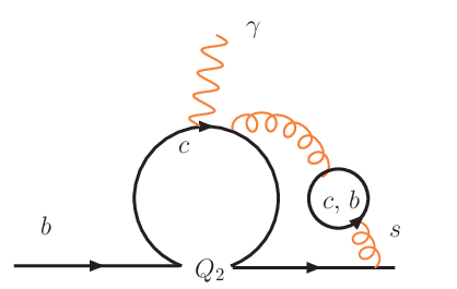
Upon reducing the set of scalar integrals involved in the calculation of diagrams with a $Q_{2}$ insertion, of which a sample is shown in FIG. 1, we are left with a set of $18$ master integrals in the case with a massless quark loop insertion into the gluon propagator, $47$ master integrals in the case with a massive b-quark loop insertion and $38$ for the c-quark case. These master integrals have been calculated by combining two different approaches.

In the first approach, we have used the Mellin-Barnes technique [24, 25], which relies on the identity

$$\frac{1}{(X+Y)^{\lambda}}=\int_{\beta-i\infty}^{\beta+i\infty}\frac{Y^{z}}{X^{\lambda+z}}\frac{\Gamma(\lambda+z)\Gamma(-z)}{\Gamma(\lambda)}\frac{\mbox{d}z}{2\pi i},$$ (7)

where $-{\rm Re}\,\lambda<\beta<0$. With this relation a sum of terms raised to some power is replaced with a product of factors. We have derived our MB representations for the master integrals using the automated package [26], and used the MB package of ref. [27] for their analytic continuation. In the case where the inserted quark loop into the gluon propagator is massless, we have used two methods. In the first, we have performed an expansion in the quark mass ratio $z=m_{c}^{2}/m_{b}^{2}$ by closing contours. The coefficients of this expansion were given by (at most) one-dimensional MB integrals which have subsequently been expressed as a sum over residues and resummed with the help of XSummer [28]. Our result for the matrix element of $Q_{2}$ using this method is in full agreement with [20]. It is also consistent with the second method, where the exact $z$-dependence was retained and a numerical integration of the MB representations was performed using the MB package.

Due to poor convergence, it turned out not to be possible to compute all the master integrals that occur in diagrams with a massive quark loop insertion with the help of MB representations. For these particular cases, we have used a second approach based on the method of differential equations. Using the fact that the master integrals $V_{i}(z,\epsilon)$ (after rescaling by a trivial factor) are functions of $\epsilon$ and the mass ratio $z$ or its inverse $y=z^{-1}$, respectively, a system of differential equations has been generated,

$$\frac{d}{dy}V_{i}(y,\epsilon)=A_{ij}(y,\epsilon)V_{j}(y,\epsilon),$$ (8)

where the right-hand side was again expressed through master integrals with the help of relations obtained from the reduction. The block-triangular matrix $A_{ij}(y,\epsilon)$ is composed of rational functions of $\epsilon$ and $y$.

The solution of this system for arbitrary values of $y$ proceeded in two steps. First, an expansion in $\varepsilon$ and $y$ for $\epsilon,\,y\rightarrow 0$ was performed with the ansatz

$$V_{i}(y,\epsilon) = \sum_{nmk}c_{inmk}\epsilon^{n}y^{m}\log^{k}y,\quad n,m=-3,-2,\dots;\;\;k=0,\dots,3+n\,\Theta(n)$$ (9)

and the coefficients were calculated recursively up to high powers of $y$ [29]. In this limit, $m_{c}^{2}\gg m_{b}^{2}$ and the initial conditions correspond to vertex diagrams that can be derived in an automated way from diagrammatic large-mass expansions. With this series at hand we were able to compute the master integrals for $y\ll 1$ with high precision. In the second step a numerical integration of the $\epsilon$-expanded system into the physical region, $y>1$, was carried out using the high precision values at a starting point $y\ll 1$. For this task, we have used the Fortran package ODEPACK [30], which allows for numerical solutions of huge systems of differential equations. To avoid points of numerical instability on the real axis, the integration path has been shifted into the complex plane.

Besides the bare three-loop matrix elements, we also needed matrix elements of two types of counterterms: those coming from the renormalization of the strong coupling constant $\alpha_{s}$ (known from the QCD beta function [31, 32]), and those due to the mixing of $Q_{2}$ into other operators. For the corresponding details, we refer the reader to [20]. We just mention here that the renormalization constants used for the renormalization of the diagrams with a massless quark loop insertion into the gluon propagator are the same as those used for the renormalization of the diagrams with a massive quark loop insertion, because all the needed renormalization constants were derived in the $\overline{MS}$-scheme and are therefore mass independent.

3 Results

Figure 2: Plot of $\mbox{Re}\langle s\gamma|Q_{2}|b\rangle^{(2),0}_{n_{f}}$ for one massless flavor and $\mu_{b}=m_{b}$. The dashed vertical line corresponds to the central value $m_{c}^{2}/m_{b}^{2}=0.068$.

We now present the results for the amplitudes of the three different quark loop insertions with the following normalization

$$\langle s\gamma|Q_{2}|b\rangle_{{\mathcal{O}}(\alpha_{s}^{2}n_{f})}=\left(\frac{\alpha_{s}}{4\pi}\right)^{2}\,\frac{e}{8\pi^{2}}\,m_{b}\,\,n_{f}\,\langle s\gamma|Q_{2}|b\rangle^{(2),M}_{n_{f}}\,\,\bar{u}_{s}\,R\,\varepsilon\hskip-4.49997pt/\,q\hskip-4.49997pt/\,u_{b}$$ (10)

where $m_{b}$ denotes the b-quark pole mass, $\varepsilon$ and $q$ are the photon polarization and momentum, $R=(1+\gamma_{5})/2$ is the right handed projection operator, and $n_{f}$ is the number of active flavors of a given mass. The superscript $(2)$ counts the powers of $\alpha_{s}$ and $M=\,$($0,\,m_{b}\,\mbox{or}\,m_{c}$) denotes the mass of the quark running in the loop inserted into the gluon propagator.

It is important that there is no need for a b-quark mass renormalization in our calculation, so we use the different schemes as guided by the complete calculation, and thus turn to the 1S mass [33] for our final study.

All our subsequent results are given in the form of fitting formulae that cover the whole interesting range of variation of $z$. With the current input given in Table 1, and allowing for a 3 sigma variation of $m_{c}(m_{c})$ and $m_{b}^{1S}$, this corresponds to $z\in[0.017,0.155]$. In the plots of Fig. 2 and Fig. 3, we also show the central value, which is currently $z=0.068$.

Input parameter	experimental value
$m_{b}^{1S}$	$(4.68\pm 0.03)\;{\rm GeV}$ [34]
$m_{c}(m_{c})$	$(1.224\pm 0.017\pm 0.054)\;{\rm GeV}$ [35]

Table 1:  Experimental inputs relevant for the present calculation

In the case of a massless quark loop insertion we agree with the previous calculation [20]. Nevertheless we present here a fitting formula for easier comparison with our new results

$$\mbox{Re}\langle s\gamma|Q_{2}|b\rangle^{(2),0}_{n_{f}} = 9.080-0.7624\,z-5.069\,z^{2}+12.61\,z\,\ln z$$ (11)

$$+ (-9.679+5.157\,z+1.726\,z^{2}-16.18\,z\,\ln z)\ln(m_{b}/\mu)$$

$$+ \frac{800}{243}\,\ln^{2}(m_{b}/\mu)$$

In Fig. 2 we show the data points used to obtain the fit function together with the result Eq. 11. Motivated by the presence of logarithms in the small $z$ expansion, we have included terms proportional to $z\,\ln z$ above, and in equations (12) and (13) below, which improved the quality of the fit significantly. As it stands, our fit function reproduces the exact values with a relative precision of at least $10^{-4}$.

Our result for the contribution of the diagrams with a massive b-quark loop insertion is given by the fitting formula of the same relative precision as above

$$\mbox{Re}\langle s\gamma|Q_{2}|b\rangle^{(2),m_{b}}_{n_{f}} = -1.836+2.608\,z+0.8271\,z^{2}-2.441\,z\,\ln z$$ (12)

$$+ (-9.595+5.157\,z+1.726\,z^{2}-16.18\,z\,\ln z)\ln(m_{b}/\mu)$$

$$+ \frac{800}{243}\,\ln^{2}(m_{b}/\mu)$$

which is plotted in Fig. 3(a). It is interesting to note that the massless approximation overestimates the massive result by a factor of $6$ and, moreover, has the opposite sign. This points to an expected decoupling like effect. Remark, however, that the scale dependence is just as strong as in the massless case.

When the massless approximation is confronted with the result for the charm quark loop insertion, one still observes noticeable differences as shown in Fig. 3(b). The obtained fitting formula of relative precision of $10^{-4}$ is

$$\mbox{Re}\langle s\gamma|Q_{2}|b\rangle^{(2),m_{c}}_{n_{f}} = 9.099+13.20\,z-19.68\,z^{2}+25.71\,z\,\ln z$$ (13)

$$+ (-9.679+13.62\,z-13.94\,z^{2}-12.98\,z\,\ln z)\ln(m_{b}/\mu)$$

$$+ \frac{800}{243}\,\ln^{2}(m_{b}/\mu)$$

When $z$ approaches $0$ both Eq. 11 and Eq. 13 tend approximately to the same value, as it should be. The residual difference is due to the quality of the fit outside the validity range, and the steepness of the curves in Fig. 3.

(a)

(b)

Figure 3: Plots of $\mbox{Re}\langle s\gamma|Q_{2}|b\rangle^{(2),M}_{n_{f}}$ as function of $m_{c}^{2}/m_{b}^{2}$ with $M=m_{b}$ (a) and $M=m_{c}$ (b) and $\mu_{b}=m_{b}$. For comparison, we also show the $M=0$ case.

Let us finally comment on the renormalization group logarithms in Eqs. 11 to 13. It has already been shown in the massless case in [22] that the single logs can be expressed through the $a(z)$ and $b(z)$ functions known from the NLO calculation [36]. In fact the exact expression for the coefficient of $\log(m_{b}/\mu)$ in this case is

$$\frac{8}{3}\left(\Re\left(a(z)+b(z)\right)-\frac{290}{81}\right).$$ (14)

Using the RGE one can show that the coefficient of the same log in Eq. 12 is

$$\frac{8}{3}\left(\Re\left(a(z)+b(z)+b(1)\right)-\frac{290}{81}\right),$$ (15)

and similarly for Eq. 13

$$\frac{8}{3}\left(\Re\left(a(z)+2b(z)\right)-\frac{290}{81}\right).$$ (16)

4 Conclusions

In this paper, we have presented a calculation of the ${\mathcal{O}}(\alpha_{s}^{2}n_{f})$ contribution to the charm quark mass dependent matrix elements of the $\bar{B}\to X_{s}\gamma$ decay. In [20], a similar calculation was done as a mass expansion in the ratio $z=m_{c}^{2}/m_{b}^{2}$ assuming that the b and c quarks inside the fermionic loop inserted into the gluon propagator are massless. The results have then been used to estimate the complete corrections of ${\mathcal{O}}(\alpha_{s}^{2})$ to the matrix elements $\langle s\gamma|Q_{1,2}|b\rangle$ by replacing $n_{f}$ with $-\frac{3}{2}\beta_{0}$, i.e. following the naive non-abelianization procedure. They form an important part of the NNLO contributions used in the recent theoretical estimate of the branching ratio ${\mathcal{B}}(\bar{B}\to X_{s}\gamma)$ [6]. Our goals were firstly to provide an independent check of the ${\mathcal{O}}(\alpha_{s}^{2}n_{f})$ corrections for massless quarks, and secondly to check the validity of the massless approximation by keeping the full mass dependence. These goals have been reached, and our result in the massless approximation, which we have obtained as a mass expansion in $z$ as well as an exact evaluation in terms of multi-fold MB integrals, confirms the findings of [20]. However, although the massless approximation reproduces the contribution of the diagrams with a massive c-quark loop insertion reasonably well, it is not justified for the diagrams with a massive b-quark. Neglecting the mass of this particle leads to an estimate of its contribution that is $6$ times larger than its true value and moreover has the opposite sign. Of course, since this effect comes from a single quark family its impact on the branching ratio is rather mild. It turns out that, when compared with the interpolation from [22], one finds an enhancement between one and two percent, depending on the renormalization scale $\mu$.

Appendix A Contributions in the limit $m_{c}\gg m_{b}$

During our calculation we also derived the large $m_{c}$ limit of all the contributions. In the massless case, we agree with [22]. For the two massive cases, we have (with $\mu=m_{b}$)

$$\langle s\gamma|Q_{2}|b\rangle^{(2),m_{b}}_{n_{f}} = 4.25648+0.503085\,\ln z+0.888889\,\ln^{2}z$$

$$+ \frac{1}{z}\,(-0.725053-1.80916\,\ln z+0.0938272\,\ln^{2}z)$$

$$+ \frac{1}{z^{2}}\,(-1.39486-0.968501\,\ln z-0.147443\,\ln^{2}z)+{\mathcal{O}}\left(\frac{1}{z^{3}}\right),$$

and

$$\langle s\gamma|Q_{2}|b\rangle^{(2),m_{c}}_{n_{f}} = 1.67932+0.526749\,\ln z+0.823045\,\ln^{2}z$$

$$+ \frac{1}{z}\,(0.20839+0.11775\,\ln z+0.128395\,\ln^{2}z)$$

$$+ \frac{1}{z^{2}}\,(-0.0360638-0.0470166\,\ln z+0.0324515\,\ln^{2}z)+{\mathcal{O}}\left(\frac{1}{z^{3}}\right).$$