On the location of the surface-attached globule phase in collapsing polymers.

Abstract

We investigate the existence and location of the surface phase known as the “Surface-Attached Globule” (SAG) conjectured previously to exist in lattice models of three-dimensional polymers when they are attached to a wall that has a short range potential. The bulk phase, where the attractive intra-polymer interactions are strong enough to cause a collapse of the polymer into a liquid-like globule and the wall either has weak attractive or repulsive interactions, is usually denoted Desorbed-Collapsed or DC. Recently this DC phase was conjectured to harbour two surface phases separated by a boundary where the bulk free energy is analytic while the surface free energy is singular. The surface phase for more attractive values of the wall interaction is the SAG phase. We discuss more fully the properties of this proposed surface phase and provide Monte Carlo evidence for self-avoiding walks up to length 256 that this surface phase most likely does exist. Importantly, we discuss alternatives for the surface phase boundary. In particular, we conclude that this boundary may lie along the zero wall interaction line and the bulk phase boundaries rather than any new phase boundary curve.

The phase transitions of a single isolated polymer in solution continue to attract attention as single polymers are fundamental components in more complicated modelling scenarios and these transitions are not yet fully understood. The collapse transition [1] mediated by the intra-polymer attractive interactions and the adsorption transition [2] when a polymer is attached to a sticky wall, are two of the key transitions that have been well studied. The situation when both transitions can occur in the same system has been studied less intensely due to the difficulty of numerical work such as Monte Carlo simulations when two independent parameters compete. However, with the advent of more powerful computers and sophisticated algorithms this situation has received some attention.

The standard lattice model for polymers is the self-avoiding walk (SAW) with the sites of the walk called monomers. The intra-polymer attraction is modelled by a potential energy $\varepsilon_{p}$ associated with monomers that are nearest-neighbours on the lattice. These instances will be referred to as (nearest-neighbour) contacts. To consider adsorption a wall is introduced, so that the polymer is restricted to one side of the wall, or may visit the wall, with one end of the polymer (SAW) attached to the wall. Any monomer which visits the wall, other that the one fixed on the wall, is given a potential energy $\varepsilon_{w}$. These monomers will be referred to as visits. Various different phases are conjectured to exist at different values of the ratio of the two energies and the temperature (see below). We shall restrict our discussion to three dimensions, as this is where more complex behaviour can occur (rather than two dimensions, where more is known due to exactly solved models and conformal field theory).

Consider the simple cubic lattice and the half space $z\geq 0$. Consider an $n$-step self-avoiding walk $\varphi$ with one end fixed at the origin. We define two Boltzmann weights $\omega_{p}=e^{-\varepsilon_{p}/k_{B}T}$ and $\omega_{w}=e^{-\varepsilon_{w}/k_{B}T}$ where $k_{B}$ is Boltzmann’s constant and $T$ is the temperature. Therefore, when $\omega_{w}>1$, $\omega_{w}=1$ and $\omega_{w}<1$ the interaction of the walk with the wall is attractive, neutral, and repulsive, respectively. When $\omega_{p}>1$, $\omega_{p}=1$ and $\omega_{p}<1$ the intra-polymer interaction is attractive, neutral, and repulsive, respectively.

The partition $Z_{n}(\omega_{p},\omega_{w})$ of the model (see Figure 1) is defined as

$$Z_{n}(\omega_{p},\omega_{w})=\sum_{\varphi\in\Omega_{n}}\omega_{p}^{m_{p}(\varphi)}\omega_{w}^{m_{w}(\varphi)}\;,$$ (1)

where $\Omega_{n}$ is the set of all $n$-step SAW restricted to the half space $z\geq 0$, $m_{p}(\varphi)$ is the number of contacts in the walk $\varphi$, and $m_{w}(\varphi)$ is the number of wall visits of the walk $\varphi$. The bulk thermodynamic (reduced) free energy is given by the limit

$$f_{b}(\omega_{p},\omega_{w})=-\lim_{n\rightarrow\infty}\frac{1}{n}\log\big(Z_{n}(\omega_{p},\omega_{w})\big)\;.$$ (2)

Figure 1: A 9-step SAW ($n=9$) attached to a wall with three visits ($m_{w}=3$) to the wall and two nearest neighbour contacts ($m_{w}=2$, shown as double helices).

The bulk phase diagram is determined by the analytic structure of $f_{b}(\omega_{p},\omega_{w})$. This phase structure was studied in a series of papers [3, 4, 5] where a schematic phase diagram was proposed (see Figure 2). To discuss this diagram it is worth considering two order parameters. Firstly let us define the “internal density” $\bar{\rho}_{p}$ as

$$\bar{\rho}_{p}=\lim_{n\rightarrow\infty}\rho_{p}(n)=\lim_{n\rightarrow\infty}\frac{n}{R_{g}^{3}(n)}\;,$$ (3)

where $R_{g}(n)$ is the radius of gyration. Secondly we define the density of wall visits $\bar{\rho}_{w}$ as

$$\bar{\rho}_{w}=\lim_{n\rightarrow\infty}\rho_{w}(n)=\lim_{n\rightarrow\infty}\frac{\langle m_{w}\rangle}{n}\;,$$ (4)

where $\langle m_{w}\rangle$ is the ensemble average of the number of visits to the wall.

Figure 2: Schematic bulk phase diagram for collapsing adsorbing walks in three dimensions showing the four phases Desorbed-Extended (DE), Desorbed-Collapsed (DC), Adsorbed-Extended (AE) and Adsorbed-Collapsed (AC). Also shown are the dashed lines where simulations were performed.

For any ratio of wall to intra-polymer energies at high temperatures, the polymer is in the excluded volume state and is entropically repulsed from the wall. It is expected that $R_{g}(n)\sim n^{\nu}$ as $n\rightarrow\infty$, where the three-dimensional excluded volume value has been estimated as $\nu=\nu_{3}\approx 0.5874(2)$ [6]. The average number of visits is expected to behave as $\langle m_{w}\rangle=o(n)$ (in fact, it is expected to be bounded): this has been numerically verified. Hence for $\omega_{w}=\omega_{p}=1$ we have $\bar{\rho}_{w}=\bar{\rho}_{p}=0$. Since $\bar{\rho}_{p}=0$ the polymer is referred to as “Extended” and since $\bar{\rho}_{w}=0$ the polymer is referred to as “Desorbed”.

Now let us consider fixed $\omega_{w}=1$ and varying $\omega_{p}$. That is, we consider the collapse transition of a polymer fixed to a non-interacting wall as the intra-polymer attraction is increased. As the temperature is lowered (increasing the effect of the attraction) the collapse transition is understood to occur at the $\theta$-point, where for high temperatures $\bar{\rho}_{p}=0$ (the Extended phase), while for low temperatures $\nu=1/3$ and $\bar{\rho}_{p}>0$ (the Collapsed phase): this is expected to be a second order phase transition [1]. In both two and three dimensions this transition has been extensively studied (see for example [7] and references therein).

On the other hand, if we consider fixed $\omega_{p}=1$ as the temperature is lowered ($\omega_{w}$ is increased), the wall density is expected to change from $\bar{\rho}_{w}=0$ (Desorbed phase) for high temperatures to $\bar{\rho}_{w}>0$ (Adsorbed phase) for low temperatures. This adsorption transition is also expected to be second order [2] and also has been well studied with this description being numerically well verified (again also see [7]). Note that for low temperatures the polymer is in a two-dimensional excluded volume state, where $\nu=\nu_{2}=3/4$ [8]. We know that a two-dimensional polymer can also admit a collapse transition, so one naturally can conjecture a state where the polymer is both adsorbed with $\bar{\rho}_{w}>0$ and two-dimensionally collapsed. A suitable two-dimensional order parameter to describe this transition is

$$\bar{\sigma}_{p}=\lim_{n\rightarrow\infty}\sigma_{p}(n)=\lim_{n\rightarrow\infty}\frac{n}{R_{g}^{2}(n)}\;.$$ (5)

When considering the full problem where both $\omega_{p}$ and $\omega_{w}$ can vary Vrbová and Whittington [3, 4] conjectured, and numerically verified, a phase diagram with precisely these four phases: Desorbed-Extended (DE) phase with $\bar{\rho}_{p}=0$ and $\bar{\rho}_{w}=0$ for small $\omega_{p}$ and $\omega_{w}$, Desorbed-Collapsed (DC) phase with $\bar{\rho}_{p}>0$ and $\bar{\rho}_{w}=0$ for large $\omega_{p}$ and (relatively) small $\omega_{w}$, Adsorbed-Extended (AE) with $\bar{\sigma}_{p}=0$ and $\bar{\rho}_{w}>0$ for (relatively) small $\omega_{p}$ and large $\omega_{w}$, and Adsorbed-Collapsed (AC) with $\bar{\sigma}_{p}>0$ and $\bar{\rho}_{w}>0$ for large $\omega_{p}$ and $\omega_{w}$.

Let us return to the bulk Desorbed-Collapsed phase where $\bar{\rho}_{p}>0$ and $\bar{\rho}_{w}=0$. One may now ask: how does $\bar{\rho}_{w}$ approach zero as the length is increased or, rather equivalently, how does the average number of wall visits $\langle m_{w}\rangle$ scale as $n$ is increased. It is believed (see below) that in the Desorbed-Extended phase $\langle m_{w}\rangle=O(1)$, that is it is bounded. One may be tempted to assume that this is also the case in the Desorbed-Collapsed phase. However, recent work [9, 10, 11] suggests that two different asymptotic behaviours can occur inside the latter.

To understand this, let us consider the finite-sized extensive (reduced) free energy $F(n;\omega_{p},\omega_{w})=-\log(Z_{n})$. From thermodynamics we expect that

$$F(n;\omega_{p},\omega_{w})=f_{b}(\omega_{p},\omega_{w})n+o(n)\;,$$ (6)

and as stated above it is the analytic structure of the bulk free energy $f_{b}(\omega_{p},\omega_{w})$ that defines the phases of our model. Drawing on the standard polymer scaling in [12], the behaviour of the finite-size free energy in the DE phase is given by

$$F(n;\omega_{p},\omega_{w})=f_{b}(\omega_{p},\omega_{w})n+(\gamma_{1}-1)\log(n)+O(1)\;,$$ (7)

where $\gamma_{1}$ is an universal constant for the DE phase (an exponent, in fact). In the DC phase the scaling is expected to behave as

$$F(n;\omega_{p},\omega_{w})\sim f_{b}(\omega_{p},\omega_{w})n+f_{s}(\omega_{p},\omega_{w})n^{2/3},$$ (8)

where we have a surface free energy $f_{s}(\omega_{p},\omega_{w})$. This behaviour arises as the polymer assumes a dense liquid-like drop with a well defined surface that has area $\propto n^{2/3}$. We reiterate that this “surface” is not the wall but rather the surface of the liquid-like polymer drop. In the extended phase the polymer does not have a well defined surface and so $f_{s}=0$ as in equation ??.

Importantly, the mean number of wall visits $\langle m_{w}\rangle$ can be calculated in the usual way as

$$\langle m_{w}\rangle=-\frac{\partial F(n;\omega_{p},\omega_{w})}{\partial\log(\omega_{w})}\;.$$ (9)

Hence

$$\langle m_{w}\rangle\sim-\frac{\partial f_{b}(\omega_{p},\omega_{w})}{\partial\log(\omega_{w})}n-\frac{\partial f_{s}(\omega_{p},\omega_{w})}{\partial\log(\omega_{w})}n^{2/3}\;.$$ (10)

Since we assume that in both the Desorbed-Extended and Desorbed-Collapsed phases $\langle m_{w}\rangle=o(n)$, it is clear that $f_{b}(\omega_{p},\omega_{w})$ should not be depend on $\omega_{w}$. Hence we have

$$\langle m_{w}\rangle\sim-\frac{\partial f_{s}(\omega_{p},\omega_{w})}{\partial\log(\omega_{w})}n^{2/3}\;.$$ (11)

In the Desorbed-Extended phase $f_{s}(\omega_{p},\omega_{w})=0$, which derives (with some other weak assumptions) the $\langle m_{w}\rangle=O(1)$ result for that phase. The question that then arises is the behaviour of $f_{s}(\omega_{p},\omega_{w})$ for the Desorbed-Collapsed phase.

In [9, 10, 11] it was suggested that the Desorbed-Collapsed phase accommodates two different behaviours: one where $f_{s}(\omega_{p},\omega_{w})$ depends on $\omega_{w}$ and so $\langle m_{w}\rangle\sim n^{2/3}$, which was dubbed the “Surface Attached Globule” or SAG, and one in which $f_{s}(\omega_{p},\omega_{w})$ is independent of $\omega_{w}$, so that $\langle m_{w}\rangle=O(1)$ as in the Desorbed-Extended phase. We shall refer to this second situation as the “Fully Detached Globule”. Physically the SAG phase can be pictured as the liquid drop partially wetting the wall, while the FDG is the state where the wall is dry. (The Adsorbed-Collapsed phase is the equivalent of a fully wet state.) This implies a surface phase transition with a singularity in $f_{s}(\omega_{p},\omega_{w})$ as $\omega_{w}$ is varied, whereas $f_{b}(\omega_{p},\omega_{w})$ is analytic at the same point and no bulk transition occurs.

The evidence given in [9, 10, 11] for the two ‘surface’ states was based on the analysis of relatively short exact enumeration data and some analysis of a directed walk model in two dimensions. It is therefore important to test this conjecture with data from longer walks. In this paper we have simulated, using a recently developed Monte Carlo algorithm [13], the model described above along various lines in the parameter space for lengths up to 256. In a previous paper [14] we considered the bulk phase diagram and various low temperature finite size features.

In [10] the boundary between the FDG and SAG was conjectured (see Figure 3 (a)). Using a zero temperature argument [10, 14], it is easy to see that for infinite $\omega_{p}$ the transition from FDG to SAG occurs at $\omega_{w}=1$. However, the question arises as to the form of the phase boundary for finite $\omega_{p}$. In [10] it was conjectured that for finite $\omega_{p}$ (but large enough so that the polymer is collapsed) the boundary occurs at values of $\omega_{w}$ greater than one. Hence, with small but finite attractive wall potential the polymer is expected to still be in the FDG state. On the other hand, if there is no entropic penalty to be paid for the globule to sit on the wall, this gives rise to an alternative hypothesis for the FDG-SAG boundary as shown in Figure 3 (b).

Figure 3: Hypothetical boundary for the surface phase transitions. (a) conjectured in [10]. (b) is an alternative that is suggested in this paper.

We note that the phase boundary is unlikely to lie in the region for $\omega_{w}<1$; here the wall is repulsive and does not increase the surface entropy of the polymer, so one may argue that typical configurations have very few visits to the wall. Hence one conjectures that for $\omega_{w}<1$ the surface free energy $f_{s}(\omega_{p},\omega_{w})$ is independent of $\omega_{w}$ and $\langle m_{w}\rangle=O(1)$. The central question therefore is whether or not the polymer-drop partially wets the wall as soon as the wall potential becomes attractive. In the original hypothesis in Figure 3 (a), a sufficiently attractive wall is required before the polymer-drop partially wets the wall. The alternative proposed in Figure 3 (b) conjectures that any attractive potential at the wall will induce the polymer-drop to partially wet the wall.

So as to delineate the SAG-FDG phase boundary and to test for the existence of the SAG phase, we have studied three lines in the phase diagram (see Figure 2) . One line at $\omega_{p}=2.0$ was chosen since the $\theta$ point is expected to be around $\omega_{p}=1.5$ at the lengths considered here, and so by fixing $\omega_{p}=2.0$ and varying $\omega_{w}$ one explores the Desorbed-Collapsed phase. We note that the position of the collapse transition should not move as $\omega_{w}$ is varied [4]. To further consider the difference between attractive and repulsive wall interactions on the Desorbed-Collapsed phase, we have also simulated along lines $\omega_{w}=0.8$ (repulsive wall visits) and $\omega_{w}=1.3$ (attractive wall visits). The second of these lines also allows us to search for the surface phase boundary proposed in Figure 3 (a). Note that the position of the adsorption transition for small $\omega_{p}$ moves little as $\omega_{p}$ is varied.

In order to explore the Desorbed-Collapsed phase, we have used the FlatPERM Monte Carlo algorithm [13]. This algorithm estimates the density of states directly and so allows us to compute the partition function and related quantities for a wide range of $\omega_{p}$ and $\omega_{s}$. The memory required to store the density of states grows with the cube of the length and so we were restricted to SAWS of maximum length 256. Each simulation sampled approximately $10^{9}$ confirmations. To reduce errors we performed 25 independent simulations and combined the resulting data.

Before we discuss the subtleties of the surface phenomena of the SAG and FDG phases we first verify that our simulations were correctly identifying the bulk phases. To do this we estimated the average end-to-end distance of the polymer which has been established to scale in the same manner as the (more computationally costly to estimate) radius of gyration. Hence we could estimate the size exponent $\nu$ at various points. This confirms earlier work [4]. We considered the point $(\omega_{p},\omega_{w})=(1,1)$, which is in the Desorbed-Extended phase, and so should have $\nu\approx 0.59$: we find an estimate 0.60(2). Next, for the point $(\omega_{p},\omega_{w})=(1,2)$ which is expected to be in the Adsorbed-Extended phase and so should have $\nu=3/4$ we find an estimate 0.75(1). Similarly, for the points $(\omega_{p},\omega_{w})=(2,0.8)$ and $(2,1.3)$ which are in the Desorbed-Collapsed phase (and we identify below to be in the FDG surface and SAG surface phases respectively) and so should have $\nu=1/3$ we find equal estimates 0.33(2).

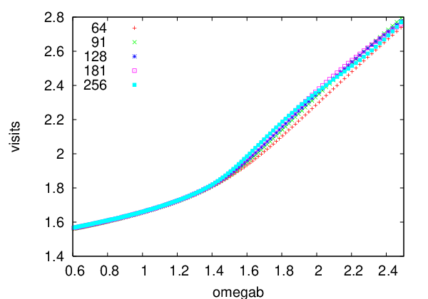
We begin our discussion of the surface phenomena by verifying the existence of the SAG phase. Let us consider the lines $\omega_{w}=1.3$ (attractive wall visits) and $\omega_{w}=0.8$ (repulsive wall visits). In Figure 4, the mean number of visits $m_{w}(n;\omega_{p},1.3)$ divided by $n^{2/3}$ is plotted against $\omega_{p}$ for $1.0\leq\omega_{p}\leq 3.0$ and $n=64$, $91$, $128$, $181$, and $256$. The quantity $m_{w}(n)/n^{2/3}$ would be expected to converge to a finite (non-zero) value only in the SAG phase. While there are clearly some corrections to scaling still evident at these lengths, $m_{w}/n^{2/3}$ seems to be convergent to a non-zero value for $\omega_{p}\gtrsim 1.5$, which is the rough location of the collapse transition at this length (the thermodynamic location has been estimated to be near $1.3$). We have also checked that for $\omega_{p}<<1.5$ (that is, in the DE bulk phase) $m_{w}$ converges to a finite value. Hence the (finite-size location) bulk phase transition at $1.5$ signifies a change in the length scaling of $m_{w}(n)$ from $n^{0}$ for small $\omega_{p}$ (DE bulk phase) to $n^{2/3}$ for large $\omega_{p}$ (DC bulk phase).

Figure 4: The mean number of visits divided by $n^{2/3}$ against $\omega_{p}>1$ for fixed $\omega_{w}=1.3$.

In Figure 5, the raw mean number of visits $m_{w}(n;\omega_{p},0.8)$ is plotted against $\omega_{p}$ for $1.0\leq\omega_{p}\leq 3.0$ and $n=64$, $91$, $128$, $181$, and $256$. As with $\omega_{w}=1.3$ one expects that for $\omega_{p}<1.5$ (DE bulk phase) that $m_{w}(n)$ will converge to a finite value as $n$ is increased and indeed this is the case. Additionally, the quantity $m_{w}(n)$ would be expected to converge to a finite (non-zero) value in the FDG phase. It appears that the collapse transition at around $\omega_{p}=1.5$ only effects the value of $\lim_{n\rightarrow\infty}m_{w}(n)$ but not whether it is finite or not. There is no indication of a change of length scaling when varying $\omega_{p}$.

Figure 5: The mean number of visits against $\omega_{p}$ for fixed $\omega_{w}=0.8$.

In Figure 6, the variance of the number of visits is plotted against $\omega_{p}$ for $\omega_{w}=1.3$ (a) and $\omega_{w}=0.8$ (b). In (a) a single peak in the variance is developing around $\omega_{p}=1.4$ as the length is increased, whereas in (b) no such peak is developing. We conclude a wall visit transition is occurring at around the same place the bulk contact transition occurs when $\omega_{w}=1.3$ but not when $\omega_{w}=0.8$.

Figure 6: Plot of the variance in the number of visits vs $\omega_{p}$ for $\omega_{w}=1.3$ (a) and $\omega_{w}=0.8$ (b). This clearly shows a difference between SAG and FDG.

We now turn to considering analysis of the line $\omega_{p}=2.0$. We first reinforce the analysis of Figure 4 and 5 by plotting the mean number of visits divided by $n^{\delta}$ along the line $\omega_{p}=2.0$. We see that using $\delta=0$ we identify the FDG regime for $\omega_{w}<1$ in Figure 7 (a). We also identify the SAG regime by using $\delta={2/3}$ in Figure 7 (b) for $1\lesssim\omega_{w}$ and at least $\omega_{w}<2$, but probably for large $\omega_{w}$ also. Finally the Adsorbed-Extended phase can be seen for $\omega_{w}>3$ where $\delta=1$.

Figure 7: Plot of the mean number of visits divided by $n^{\delta}$ vs $\omega_{w}$ for $\omega_{p}=2.0$. (a) shows the scaling in the FDG regime with $\delta=0$. (b) shows the scaling in the SAG regime with $\delta=2/3$. (c) shows the scaling in the thermodynamic adsorbed extended phase with $\delta=1$.

Considering the variance in the number of contacts (Figure 8), the bulk adsorption transition can be seen as a peak developing around $\omega_{w}\approx 2.5$, while another smaller peak can be identified just above $1.0$ (see Figure 9). While one might try to extrapolate the peak positions in Figure 9 to find the thermodynamic limit position, we find that our data is consistent with a wide range of limits ranging from 0.9 up to 1.15, depending on the choice of the correction exponent used to do the extrapolation. Certainly the peaks are moving to smaller values of $\omega_{w}$ as the length is increased.

Figure 8: The variance in the number of visits vs $\omega_{w}$ at $\omega_{p}=2.0$ and length $256$. One can clearly see two peaks indicating the possibility of two transitions.

Figure 9: The variance in the number of visits vs $\omega_{w}$ at $\omega_{p}=2.0$ for different lengths around the SAG-FDG boundary.

We now return to the analysis of the line $\omega_{w}=1.3$. In Figure 10, we plot the variances in wall visits and bulk contacts for lengths $128$ and $256$ on the same figure, scaling the bulk variance so that the corresponding peak heights of the wall visit variances are roughly comparable. This enables us to make an easier comparison of the peak positions at the two lengths. We reiterate that only one peak occurs in the variance of the wall visits. If indeed this peak were associated with a surface transition occurring at a higher value of $\omega_{p}$ than the bulk transition, one would expect to see the peaks of the variance of the visits extrapolating to a higher value of $\omega_{p}$ than the peaks of the contacts variances. In both cases the peaks of the variances in wall visits occur at smaller values of $\omega_{p}$ than the peaks of the bulk contacts, and both are moving to smaller $\omega_{p}$ as the length is increased. We have investigated the scaling of the peak heights of the variances in wall visits and bulk contacts illustrated in Figure 10. As expected the peak height of the (normalised) variance of the bulk contacts is consistent with a logarithmic scaling — an effective scaling as $(\log(n))^{2.8}$ is seen (one expects for very large $n$ scaling of $((\log(n))^{3/11}$). The scaling of (normalised) variance of the surface visits is consistent with a logarithmic scaling using an effective form of $(\log(n))^{0.5}$ (or a weak power of $n^{0.1}$). Presumably, if both have logarithmic scaling this would be consistent with both peaks being associated with the bulk collapse transition. The behaviour observed does not support the scenario in Figure 3 (a). This suggests that there exists one phase transition in the thermodynamic limit that gives rise to singularities in the scaling of the contacts and the wall visits.

Figure 10: Variance in wall visits and bulk contacts at $\omega_{w}=1.3$ vs $\omega_{p}$ at lengths $128$ and $256$. Note that the peak in the variance of the visits is to the left of the peak of the variance of the number of contacts. The variance of the number of contacts has been scaled so that the peak height of a given length is approximately the same as the peak height of the variance of the number of visits at the same length.

Finally, we show typical examples of configurations of length $n=256$ in Figure 11 at the points $(\omega_{p},\omega_{w})=(2,0.8)$ and $(2,1.3)$ which we have argued are in the FDG and SAG surface phases respectively. One clearly sees a globule like conformation in both examples with a dense amorphous grouping of monomers. At $(2,0.8)$ only the monomer tethered to the wall lies in contact with the wall while at $(2,1.3)$ a fair proportion of the monomers of the surface of the globule lie on the wall as one would expect in a surface-attached globule.

Figure 11: Examples of typical configurations of length $n=256$ at the points $(\omega_{p},\omega_{w})=(2,0.8)$ (left) and $(2,1.3)$ (right).

We conclude by summarising that while we verify the existence of the SAG phase we find no indication of separate transitions other than occur in the bulk phase diagram or along zero interaction boundaries. This gives rise to a hypothesised surface phase diagram as illustrated in Figure 3 (b).

References

- [1] de Gennes P G 1979 Scaling Concepts in Polymer Physics (Ithaca: Cornell University Press)
- [2] DeBell K and Lookman T 1993 Rev. Mod. Phys. 65 87–113
- [3] Vrbová T and Whittington S G 1996 J. Phys. A 29 6253–6264
- [4] Vrbová T and Whittington S G 1998 J. Phys. A 31 3989–3998
- [5] Vrbová T and Procházka K 1999 J. Phys. A 32 5469–5475
- [6] Prellberg T 2001 J. Phys. A 34 L599–L602
- [7] Vanderzande C 1998 Lattice models of Polymers (Cambridge University Press)
- [8] Nienhuis B 1982 Phys. Rev. Lett. 49 1062
- [9] Singh Y, Giri D and Kumar S 2001 J. Phys. A. 34 L67–L74
- [10] Rajesh R, Dhar D, Giri D, Kumar S and Singh Y 2002 Phys. Rev. E. 65 056124
- [11] Mishra P, Giri D, Kumar S and Singh Y 2003 Physica A 318 171–178
- [12] Owczarek A L, Prellberg T and Brak R 1993 J. Stat. Phys. 72 737–772
- [13] Prellberg T and Krawczyk J 2004 Phys. Rev. Lett. 92 120602
- [14] Krawczyk J, Owczarek A L, Prellberg T and Rechnitzer A 2005 Europhys. Lett. 70 726–732